1 Introduction

Yang-Mills-Higgs systems admit stable topological solitons; instantons, monopoles, vortices and domain walls. When they saturate energy bounds in supersymmetric (SUSY) gauge theories, they are called Bogomol’nyi-Prasad-Sommerfield (BPS) states preserving some fraction of SUSY. There are no forces between BPS solitons in general and all of these solutions constitute moduli spaces. The ADHM construction for instantons [1] and the Nahm construction for BPS monopoles [2] were given long time ago and have been applied to a lot of subjects in physics and mathematics. In particular monopoles and instantons played crucial roles in non-perturbative dynamics in ${\cal N}=2$ and ${\cal N}=1$ SUSY gauge theories in four dimensions [3]. Contrary to these developments, it was, however, the last year that the moduli space of multiple vortices was constructed by Hanany and Tong in non-Abelian gauge theories [4, 5, 6] following the discovery of the moduli space for a single vortex [7]. There have been few discussions for explicit constructions of moduli spaces of walls; notable exceptions are the cases of ${\cal N}=1$ generalized Wess-Zumino models [8], ${\cal N}=1$ SUSY gauge theories [9, 10] and ${\cal N}=2$ SUSY gauge theories with Abelian gauge group [11, 12]. Construction for wall solutions and their moduli space in ${\cal N}=2$ SUSY non-Abelian gauge theory with eight supercharges was desired.

Recently a systematic method to construct all exact wall solutions in $U(N_{\rm C})$ gauge theory with $N_{\rm F}$ hypermultiplets in the fundamental representation, which we call non-Abelian walls, has been given in [13, 14] (see [15] for a review). Their moduli space has been completely determined to be the complex Grassmann manifold $G_{N_{\rm F},N_{\rm C}}\simeq SU(N_{\rm F})/[SU(N_{\rm C})\times SU(N_{\rm F}-N_{\rm C})\times U(1)]$ endowed with a deformed metric. One of interesting aspects is that this moduli space is a total space containing all topological sectors with different boundary conditions and with different number of walls. Moreover the construction method has been generalized in [16] to exact solutions for a set of 1/4 BPS equations which are made of walls, vortices and monopoles in the Higgs phase [17, 18, 5, 19, 20], and to those for another set of 1/4 BPS equations [5] for vortices and instantons in the Higgs phase [21].

D-branes in string theory realize SUSY gauge theories on their world-volume at low energy. Using this property non-perturbative dynamics for SUSY gauge theories was clarified by brane dynamics in several brane configurations and vice versa [22]–[27]. Also D-brane configurations are very useful tools to describe various aspects of BPS solitons in SUSY gauge theories. Instantons are realized by a D$p$-D$(p+4)$ system [28] where $k$ D$p$-branes are regarded as $k$-instantons in the effective $U(N)$ gauge theory on $N$ D$(p+4)$-branes. The ADHM conditions are obtained as the SUSY vacuum conditions in the effective $U(k)$ gauge theory on the D$p$-branes. Taking a T-dual of this configuration we obtain one made of $k$ D$(p+1)$-branes ending on $N$ D$(p+3)$-branes. This is a brane configuration for BPS monopoles [29] giving the Nahm construction in the same way. The brane configuration for vortices was realized by Hanany and Tong [4, 5] on D$p$-brane world-volume in a D$p$-D($p+2$)-D$(p+4)$-NS$5$ system. There are several advantages to consider brane configurations for analysis of BPS solitons. One advantage is that we can interpret the ADHM or other conditions for the moduli space of solitons by the F- and D-flatness conditions of SUSY vacua as stated above. For vortices the brane configuration is the only available method to construct their moduli space although there exists some ambiguity in the moduli metric [4, 6]. The other advantage is for instance that these brane configurations give solitons in non-commutative space if we turn on an NS-NS $B$-field as a background [30, 31, 32].

In this paper we give a D-brane configuration for non-Abelian walls found in [13, 14], generalizing the kinky D-brane in the type II string theories given by Lambert and Tong [33, 11] for Abelian walls in SUSY $U(1)$ gauge theory (with eight supercharges) containing $N_{\rm F}$ massive hypermultiplets in the fundamental representation and a Fayet-Iliopoulos (FI) term (see Fig. 1). Here we recall their discussion [33] briefly. In the case of massless hypermultiplets, the moduli space of vacua in the original theory is realized as a D$p$-brane world-volume theory in a D$p$-D($p+4$) system in type II string theories with a constant $B$-field perpendicular to the single D$p$-brane along the coincident $N_{\rm F}$ D$(p+4)$-branes. The effective action for the D$(p+4)$-branes with the $B$-field is a non-commutative $U(N_{\rm F})$ gauge theory whereas the D$p$-brane inside them can be regarded as a non-commutative instanton [30]. The effective theory on the D$p$-brane is the SUSY $U(1)$ gauge theory with eight supercharges containing $N_{\rm F}$ massless hypermultiplets and the FI-term proportional to the $B$-field. The moduli space of vacua in the D$p$-brane theory coincides with the ADHM moduli space for the single non-commutative instanton. Turning on masses for hypermultiplets correspond to placing D($p+4$)-branes at separated positions where mass differences determine distances of adjacent D($p+4$)-branes. (Here we consider real masses most suitable to consider 1/2 BPS walls although mass parameters can become complex for $p=3$, triplet for $p=2$ and quartet for $p=1$.) The effective theory on the single D$p$-brane has a potential due to the FI-term, from which the theory contains $N_{\rm F}$ discrete degenerate vacua corresponding to $N_{\rm F}$ positions of the D$(p+4)$-branes [33]. Multiple domain wall configuration is realized as a kinky D$p$-brane interpolating between one D($p+4$)-brane to another D($p+4$)-brane successively as illustrated in Fig. 1, where transverse modes of the D$p$-brane perpendicular to D($p+4$)-brane world-volume are parametrized by the scalar field components in the vector multiplets and those along the D($p+4$)-branes are decoupled because of single D$p$-brane. The 1/2 BPS condition allows the D$p$-brane to curve into only one direction as illustrated in Fig. 1, and this is why it is enough to consider real masses for 1/2 BPS states even in higher dimensions.

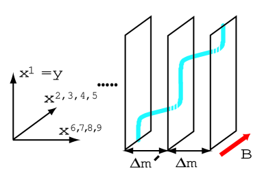
Figure 1: A kinky D-brane configuration for Abelian walls. The theory is realized on a single D$p$-brane in the background of $N_{\rm F}$ D($p+4$)-branes with separated positions and the $B$-field. Multiple walls in SUSY $U(1)$ gauge theory are realized as a single kinky D-brane interpolating between the separated D($p+4$)-branes [33, 11]. The extra coordinate is denoted by $y=x^{1}$.

Naive extension to multiple $N_{\rm C}$ D$p$-branes gives SUSY $U(N_{\rm C})$ gauge theory with eight supercharges containing an adjoint hypermultiplet in addition to $N_{\rm F}$ fundamental hypermultiplets on their world volume. The adjoint hypermultiplet describes positions of the D$p$-branes along the D$(p+4)$-brane world-volume which is not decoupled unless $N_{\rm C}=1$ discussed above; on the other hand, walls in [13, 14] are constructed in SUSY gauge theory without adjoint hypermultiplets. To remove that unwanted adjoint hypermultiplet we divide the orthogonal space ${\bf C}^{2}$ of the D$p$-branes along the D($p+4$)-brane world-volume by ${\bf Z}_{2}$. The fixed point of the ${\bf Z}_{2}$-action becomes an orbifold singularity of ${\bf C}^{2}/{\bf Z}_{2}$. Fractional D$p$-branes mean D$p$-branes with the fractional tension of the ordinary D$p$-branes, which are stuck at the singularity and a part of whose world-volume is wrapped on the shrunken cycles of the orbifold. Since they do not have degree of freedom to move in the D$(p+4)$-brane world-volume, their world-volume theory does not contain adjoint hypermultiplets corresponding to these directions. We thus realize the SUSY $U(N_{\rm C})$ gauge theory with $N_{\rm F}$ fundamental hypermultiplets without adjoint hypermultiplets on fractional D$p$-branes stuck at the orbifold singularity. Ground states of the fractional D$p$-branes can be understood as Yang-Mills instantons in the orbifold ${\bf C}^{2}/{\bf Z}_{2}$ whose singularity is blown up by $S^{2}$ to the $A_{1}$ gravitational instanton, namely, the Eguchi-Hanson space [34]. Yang-Mills instantons in gravitational instantons were constructed in [35] and were later interpreted by D-brane configurations [36]. Non-Abelian walls are realized as multiple kinky fractional D$p$-branes in such a system.

This paper is organized as follows. We give a brief review of the field theoretical results for non-Abelian walls in Sec. 2. We discuss the vacuum structure of our theory by a brane configuration of a D$p$-D($p+4$) system with ${\bf C}^{2}/{\bf Z}_{2}$ in Sec. 3. Taking a T-dual it becomes a brane configuration of Hanany-Witten [22] made of $N_{\rm C}$ D($p+1$)-branes stretched between two parallel NS$5$-branes with orthogonal $N_{\rm F}$ D($p+3$)-branes. There the s-rule (see [27] for review) is essential to count the vacua, and the Hanany-Witten effect [22, 26] explains the duality between two gauge theories with $N_{\rm C}\leftrightarrow N_{\rm F}-N_{\rm C}$ for vacuum states. Sec. 4 contains the main results in this paper. There we realize non-Abelian walls as multiple kinky fractional D$p$-branes in the original brane configuration before taking T-duality. The brane picture is very useful to read the vacua which appear when two adjacent walls are separated enough. We show that the tension of the fractional D$p$-branes correctly reproduce the tension of walls. We also calculate the tension of walls as the tension of the D($p+1$)-branes in the T-dualized configuration. We find that the s-rule and the Hanany-Witten effect are extended to kinky D-brane configurations to understand the dynamics of non-Abelian walls found in [13, 14]. The reconnection (recombination) of D$p$-branes [37] is found to occur in our kinky D$p$-brane configurations. Dimensions of the wall moduli space and its topological sectors are calculated in the brane picture. Sec. 5 is devoted to conclusion and discussions such as a brane configuration for 1/4 BPS states of wall, vortices and monopoles, a brane configuration for non-BPS walls, extension to degenerate masses or complex or more general masses for hypermultiplets and a brane configuration for a wall junction.

2 Non-Abelian Walls

In this section we briefly present field theoretical description of non-Abelian walls [13, 14, 15]. We consider five-dimensional ($D=4+1$) theory because it is the maximal dimension with massive hypermultiplets admitting domain walls. We denote space-time indices by $M,N,\cdots=0,1,2,3,4$ with the metric $\eta_{MN}={\rm diag}(+1,-1,-1,-1,-1)$. Physical bosonic fields in the vector multiplet are gauge field $W_{M}=W_{M}^{I}T_{I}$, and a real scalar field $\Sigma=\Sigma^{I}T_{I}$ in the adjoint representation of the $U(N_{\rm C})$ gauge group, with $T_{I}$ ($I=0,1,\cdots,N^{2}-1$) generators for the Lie algebra of $U(N_{\rm C})$. Physical bosonic fields in the hypermultiplets are an $SU(2)_{R}$ doublet of complex scalars represented by two $N_{\rm C}\times N_{\rm F}$ matrices $(H^{i})^{rA}\equiv(H^{irA})$ with $SU(2)_{R}$ $i=1,2$, color $r=1,\cdots,N_{\rm C}$ and flavor $A=1,\cdots,N_{\rm F}$ indices.

The bosonic Lagrangian is given by

$${\cal L}=-\frac{1}{2g^{2}}{\rm Tr}\left(F_{MN}F^{MN}\right)+\frac{1}{g^{2}}{\rm Tr}\left({\cal D}_{M}\Sigma{\cal D}^{M}\Sigma\right)+{\rm Tr}\left[{\cal D}^{M}H^{i}({\cal D}_{M}H^{i})^{\dagger}\right]-V,$$ (2.1)

where $g$ is the gauge coupling constant taken common for $U(1)$ and $SU(N)$ gauge groups. The covariant derivatives are defined by ${\cal D}_{M}\Sigma=\partial_{M}\Sigma+i[W_{M},\Sigma]$, ${\cal D}_{M}H^{i}=(\partial_{M}+iW_{M})H^{i}$, and the field strength by $F_{MN}=\frac{1}{i}[{\cal D}_{M},{\cal D}_{N}]=\partial_{M}W_{N}-\partial_{N}W_{M}+i[W_{M},W_{N}]$. The potential $V$ is given by

$$V \!\!\!= \!\!\!\frac{g^{2}}{4}{\rm Tr}\left[\left(H^{1}H^{1\dagger}-H^{2}H^{2\dagger}-c\mathbf{1}_{N_{\rm C}}\right)^{2}+4H^{2}H^{1\dagger}H^{1}H^{2\dagger}\right]$$ (2.2)

$$+{\rm Tr}\left[(\Sigma H^{i}-H^{i}M)(\Sigma H^{i}-H^{i}M)^{\dagger}\right],$$

where we have taken a triplet of the Fayet-Iliopoulos (FI) parameters to the third direction as $(0,0,c)$, using the $SU(2)_{R}$ rotation without loss of generality. Here the mass matrix is defined by $(M)^{A}{}_{B}\equiv m_{A}\delta^{A}{}_{B}$. We consider non-degenerate masses $m_{A}\neq m_{B}$ for $A\neq B$ and order them as $m_{A+1}<m_{A}$. The flavor group $SU(N_{\rm F})$ is explicitly broken to $U(1)^{N_{\rm F}-1}$ by these non-degenerate masses. For (partially) degenerate masses this flavor group is (partially) recovered.

In the massless case ($m_{A}=0$ for all $A$) the moduli space of vacua becomes the Higgs branch given by a hyper-Kähler quotient [38] resulting the cotangent bundle over the complex Grassmann manifold [39, 40]

$${\cal M}^{M=0}_{\rm vacua}\simeq T^{*}G_{N_{\rm F},N_{\rm C}}=T^{*}\left[{SU(N_{\rm F})\over SU(N_{\rm C})\times SU(\tilde{N}_{\rm C})\times U(1)}\right]\;,$$ (2.3)

with $\tilde{N}_{\rm C}\equiv N_{\rm F}-N_{\rm C}$, on which flavor symmetry $SU(N_{\rm F})$ acts as a tri-holomorphic isometry. Turning on masses for hypermultiplets, most points on ${\cal M}^{M=0}_{\rm vacua}$ are lifted leaving the discrete SUSY vacua given by

$$H^{1rA}=\sqrt{c}\,\delta^{A_{r}}{}_{A},\quad H^{2rA}=0,$$

$$\Sigma={\rm diag.}(m_{A_{1}},\,m_{A_{2}},\,\cdots,\,m_{A_{N_{\rm C}}}).$$ (2.4)

Note that there are no non-baryonic Higgs branches [41] due to the FI-parameters. These SUSY vacua (the baryonic Higgs branch) can be labeled by a set of non-zero elements $A_{r}$ as

$$\langle A_{1},\cdots,A_{N_{\rm C}}\rangle,$$ (2.5)

and therefore the number of SUSY vacua is obtained as

$${}_{N_{\rm F}}C_{N_{\rm C}}={N_{\rm F}!\over N_{\rm C}!\tilde{N}_{\rm C}!}.$$ (2.6)

For partially degenerate masses continuously degenerate vacua appear.

The BPS equations are obtained by either the 1/2 BPS condition on the fermion fields or the Bogomol’nyi completion on energy density as

$$\mathcal{D}_{y}\Sigma={g^{2}\over 2}\left(c{\bf 1}_{N_{\rm C}}-H^{1}H^{1}{}^{\dagger}+H^{2}H^{2}{}^{\dagger}\right),\hskip 14.22636pt0=-g^{2}H^{2}H^{1}{}^{\dagger},$$

$$\mathcal{D}_{y}H^{1}=-\Sigma H^{1}+H^{1}M,\hskip 14.22636pt\mathcal{D}_{y}H^{2}=\Sigma H^{2}-H^{2}M,$$ (2.7)

where we have denoted the extra dimension perpendicular to walls by $y$. The tension of multiple BPS walls, interpolating between a vacuum labeled by $\langle A_{1},\cdots,A_{N_{\rm C}}\rangle$ at $y\to+\infty$ and a vacuum $\langle B_{1},\cdots,B_{N_{\rm C}}\rangle$ at $y\to-\infty$, is obtained as

$$T_{\rm w}=c\left[{\rm Tr}\Sigma\right]^{y=+\infty}_{y=-\infty}\!\!=\!c\left(\sum_{r=1}^{N_{\rm C}}m_{A_{r}}-\sum_{r=1}^{N_{\rm C}}m_{B_{r}}\right).$$ (2.8)

To solve the BPS equations (2.7), it is convenient to define a matrix function $S(y)$ taking values in $GL(N_{\rm C},{\bf C})$ by

$$\Sigma+iW_{y}\equiv S^{-1}\partial_{y}S\,.$$ (2.9)

Then the hypermultiplets can be solved from the third and forth equations in (2.7) as

$$H^{1}(y)=S^{-1}(y)H_{0}^{1}e^{My},\quad H^{2}(y)=S^{\dagger}(y)H_{0}^{2}e^{-My}$$ (2.10)

with $H^{i}_{0}$ ($i=1,2$) $N_{\rm C}\times N_{\rm F}$ constant complex matrices. In our choice of the FI-parameter, the vacua are obtained with $H^{2}=0$ as Eq. (2.4). It was shown in Appendix C in [14] that $H_{0}^{2}$ must vanish for any wall configuration interpolating between these vacua:

$$H_{0}\equiv H_{0}^{1}\neq 0,\hskip 14.22636ptH_{0}^{2}=0$$ (2.11)

with $H_{0}$ being a rank $N_{\rm C}$ matrix, which we call the moduli matrix.

Defining an $N_{\rm C}\times N_{\rm C}$ gauge invariant matrix

$$\Omega\equiv SS^{\dagger},$$ (2.12)

the first equation in (2.7) can be rewritten as

$$\partial_{y}^{2}\Omega-\partial_{y}\Omega\Omega^{-1}\partial_{y}\Omega=g^{2}\left(c\,\Omega-H_{0}\,e^{2My}H_{0}{}^{\dagger}\right).$$ (2.13)

Once a solution $\Omega(y)$ of this equation is obtained, $S$ can be calculated by Eq. (2.12) with fixing a gauge. Then all physical quantities $H^{i}(y)$, $\Sigma(y)$ and $W_{y}(y)$ can be obtained from $S$ by Eqs. (2.9) and (2.10).

A set $(S^{\prime},H_{0}^{1}{}^{\prime})$ and another set $(S,H_{0})$ related by the following relation give the same physical quantities:

$$S^{\prime}=VS,\quad H_{0}{}^{\prime}=VH_{0},\quad$$ (2.14)

with $V\in GL(N_{\rm C},{\bf C})$. We call this transformation by $GL(N_{\rm C},{\bf C})$ the world-volume symmetry.

All moduli parameters in wall solutions are contained in the moduli matrix $H_{0}$. However the world-volume symmetry (2.14) enforces a equivalence relation on $H_{0}$, and not all of parameters in $H_{0}$ are independent. Therefore the moduli space ${\cal M}_{\rm wall}$ for wall configurations are obtained as the complex Grassmann manifold

$${\cal M}_{\rm wall}\simeq\{H_{0}|H_{0}\sim VH_{0},V\in GL(N_{\rm C},{\bf C})\}\simeq G_{N_{\rm F},N_{\rm C}}\simeq{SU(N_{\rm F})\over SU(N_{\rm C})\times SU(\tilde{N}_{\rm C})\times U(1)}\,.$$ (2.15)

In particular its real dimension is

$$\dim{\cal M}_{\rm wall}=2N_{\rm C}\tilde{N}_{\rm C}=2N_{\rm C}(N_{\rm F}-N_{\rm C}).$$ (2.16)

This moduli space contains all topological sectors with different possible boundary conditions:

$${\cal M}_{\rm wall}=\sum_{\rm BPS}{\cal M}^{\langle A_{1},\cdots,A_{N_{\rm C}}\rangle\leftarrow\langle B_{1},\cdots,B_{N_{\rm C}}\rangle}$$ (2.17)

where ${\cal M}^{\langle A_{1},\cdots,A_{N_{\rm C}}\rangle\leftarrow\langle B_{1},\cdots,B_{N_{\rm C}}\rangle}$ is defined as the topological sector with boundary conditions, $\langle A_{1},\cdots,A_{N_{\rm C}}\rangle$ at $y\to+\infty$ and $\langle B_{1},\cdots,B_{N_{\rm C}}\rangle$ at $y\to-\infty$. Therefore we call ${\cal M}_{\rm wall}$ the total moduli space for walls.

To obtain a (multiple) wall configuration in the topological sector ${\cal M}^{\langle A_{1},\cdots,A_{N_{\rm C}}\rangle\leftarrow\langle B_{1},\cdots,B_{N_{\rm C}}\rangle}$ we need to fix the world-volume symmetry (2.14) in a proper way. Any moduli matrix for such a configuration in that topological sector can be uniquely fixed as the form of

$$\hskip 52.00005ptA_{1}\hskip 31.0001ptA_{r}\hskip 27.0pt\stackrel{{\scriptstyle y\rightarrow\infty}}{{\longleftarrow}}\hskip 26.00009ptB_{1}\hskip 42.00003ptB_{r}$$

$$H_{0} = \sqrt{c}\left(\begin{array}[]{cccccccccccc}\cdots 0&1&*\cdots&*&\cdots&&\cdots*&e^{v_{1}}&0\cdots\\ &&\vdots&&&&\vdots&&&&&\\ &&\cdots 0&1&*\cdots&&\cdots&&\cdots*&e^{v_{r}}&0\cdots\\ &&\vdots&&&&\vdots&&&&&\\ &&&&\cdots 0&1&*\cdots&\cdots*&e^{v_{N_{\rm C}}}&0\cdots\\ \end{array}\right){{\small<r}}\,,$$

$$\hskip 138.00023ptA_{N_{\rm C}}\hskip 52.00005ptB_{N_{\rm C}}$$

where in the $r$-th row the left-most non-zero $(r,A_{r})$-elements are fixed to be one, the right-most non-zero $(r,B_{r})$-elements are denoted by $e^{v_{r}}(\in{\bf C}^{*}\equiv{\bf C}-\{0\}\simeq{\bf R}\times S^{1})$, and elements between them denoted by $*(\in{\bf C})$ are complex parameters which can be zero. We call this matrix the standard form of $H_{0}$. Here $A_{r}$ are ordered as $A_{r}<A_{r+1}$ using the world-volume symmetry (2.14), but $B_{r}$ cannot be ordered in general. When $B_{r}$ are not ordered some elements between 1 and $e^{v_{r}}$ must be eliminated to fix the world-volume symmetry (2.14) completely, where the positions of zeros can be uniquely determined (see Appendix B in [14]). On the other hand, when $B_{r}$ happen to be ordered all elements can be non-zero and we call that moduli matrix the generic moduli matrix in that topological sector. This implies that the generic region of the topological sector ${\cal M}^{\langle A_{1},\cdots,A_{N_{\rm C}}\rangle\leftarrow\langle B_{1},\cdots,B_{N_{\rm C}}\rangle}$ is covered by the moduli parameters in the generic moduli matrix, whereas those of the other moduli matrices cover regions with smaller dimensions which are boundaries of the generic region. Each topological sector is completely covered by patches $U^{\langle A_{1},\cdots,A_{N_{\rm C}}\leftarrow B_{1},\cdots,B_{N_{\rm C}}\rangle}$ of moduli matrices in the standard form (2) with all allowed ordering of $B_{r}$ with $A_{r}<B_{r}$. The topological sector can be decomposed as

$${\cal M}^{\langle A_{1},\cdots,A_{N_{\rm C}}\rangle\leftarrow\langle B_{1},\cdots,B_{N_{\rm C}}\rangle}=\sum_{\sigma[A_{r}\leq B_{\sigma(r)}]}U^{\langle A_{1},\cdots,A_{N_{\rm C}}\leftarrow B_{\sigma(1)},\cdots,B_{\sigma(N_{\rm C})}\rangle}$$ (2.24)

where $\sigma$ denotes an element of the permutation group acting on the ordered $B_{r}$, and the sum is taken over all allowed permutations under the condition $A_{r}\leq B_{\sigma(r)}$ for each $r$-th row. Here each pair of $U$’s does not have overlap because the standard form is unique once the ordering for $B_{r}$ is given.

It is in general so difficult to solve Eq. (2.13) explicitly. For finite gauge coupling with particular values some exact solutions are obtained for $U(1)$ gauge theories [33, 42, 43, 44]. We can obtain exact solutions with full generic moduli for non-Abelian gauge theories by taking the strong gauge coupling limit $g\to\infty$. In this limit Eq. (2.13) can be algebraically solved to give

$$\Omega_{g\to\infty}\equiv\Omega_{0}=c^{-1}H_{0}e^{2My}H_{0}{}^{\dagger}\;.$$ (2.25)

The original Lagrangian (2.1) reduces to a hyper-Kähler nonlinear sigma model on the target space $T^{*}G_{N_{\rm F},N_{\rm C}}(\simeq{\cal M}^{M=0}_{\rm vacua})$ in Eq. (2.3) with the potential term [40]. This method to obtain hyper-Kähler manifold is known as a hyper-Kähler quotient [39, 38]. The potential term can be written as square of a tri-holomorphic Killing vector [45] generated by $\sum_{A}m_{A}t_{A}$ with $t_{A}$ a $U(1)[\subset U(1)^{N_{\rm F}}]$ generator acting on $H^{irA}$ (the overall $U(1)$ is gauged away). This type of model is called a massive hyper-Kähler nonlinear sigma model and is known to admit various (composite) BPS solitons like (multiple) walls [46, 11, 12, 47], strings ending on a wall [17] and stretched between multiple walls [16], intersecting walls [48] and intersecting strings (lumps) [49].

3 Brane Configuration for Moduli Space of Vacua

3.1 Massless Hypermultiplets

First we discuss the case that all hypermultiplets are massless. Consider a D$p$-D$(p+4)$ system with $N_{\rm C}$ D$p$-branes and $N_{\rm F}$ coincident D$(p+4)$-branes in type IIA/IIB string theory. Moreover we divide the orthogonal space ${\bf C}^{2}$ perpendicular to the D$p$-branes inside the D$(p+4)$-brane world-volume by ${\bf Z}_{2}$ (to remove unwanted adjoint hypermultiplets) and turn on a constant self-dual NS-NS $B$-field on ${\bf C}^{2}/{\bf Z}_{2}$. The ALE space of the $A_{1}$-type, the Eguchi-Hanson space, is obtained by blowing up the orbifold singularity by inserting $S^{2}$. The positions of fractional D$p$-branes inside the D$(p+4)$-branes are localized at the fixed point of the orbifold singularity of ${\bf C}^{2}/{\bf Z}_{2}$ because they are D$(p+2)$-branes wrapping around $S^{2}$ which blows up the singularity. In the case of $p=1$ in the type IIB string theory, we obtain the following configuration (see Fig. 2)

$$N_{\rm C} 1 01$$ D:

$$N_{\rm F} 5 012345$$ D:

$${\bf C}^{2}/{\bf Z}_{2} \hskip 12.80373pt2345$$ ALE: (3.1)

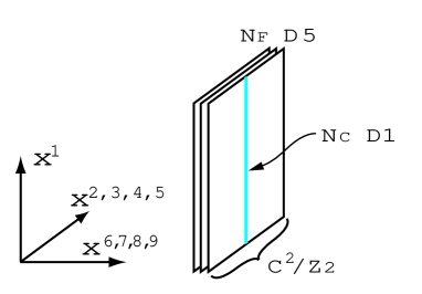
Figure 2: A D-brane configuration for massless hypermultiplets in the fundamental representation.

The $N_{\rm C}$ D$p$-branes are interpreted as instantons (with the instanton number $N_{\rm C}$) on the ALE space in the effective $U(N_{\rm F})$ gauge theory on the D$(p+4)$-branes. The moment maps of $U(N_{\rm C})$ gauge group for the ADHM moduli space of instantons in the ALE space are found by Kronheimer and Nakajima [35] to be

$$\mu_{\bf C}=IJ,\hskip 14.22636pt\mu_{\bf R}=II^{\dagger}-J^{\dagger}J$$ (3.2)

with $I$ and $J$ being $N_{\rm C}\times N_{\rm F}$ and $N_{\rm F}\times N_{\rm C}$ matrices with complex components, respectively. A set of $I$ and $J$ can be interpreted as an $N_{\rm C}\times N_{\rm F}$ matrix of hypermultiplets arisen from a string stretched between the D$p$-branes and the D($p+4$)-branes. Then the ADHM moduli space is obtained as a hyper-Kähler quotient [38], to yield

$${\cal M}^{M=0}_{\rm vacua}\simeq\{(I,J)|\mu_{\bf C}=0,\mu_{\bf R}=c\}/U(N_{\rm C})\simeq T^{*}G_{N_{\rm F},N_{\rm C}}$$ (3.3)

where $c$ is interpreted as the FI-parameter of the effective gauge theory on the fractional D$p$-branes. Eq. (3.3) is understood as the moduli space of vacua in the effective theory on the fractional D$p$-branes which coincides with the field theoretical result (2.3) [40]. Let $g_{s}$ and $l_{s}=\sqrt{\alpha^{\prime}}$ the string coupling constant and the string length, respectively. We now express the parameters in the effective gauge theory on the fractional D$p$-branes in terms of them. The FI-parameter $c$ blows up the ${\bf Z}_{2}$ orbifold singularity by inserting $S^{2}$ with the area

$$A={\rm Area}\,(S^{2})\sim c\,\,l_{s}^{p+1}$$ (3.4)

where we will determine the $g_{s}$ dependence in Eq. (4.3), below. The gauge coupling constant $g$ is given by

$$\frac{1}{g^{2}}=b\,\tau_{p+2}\,l_{s}^{2}={b\over\,g_{s}l_{s}^{p-3}}$$ (3.5)

with $\tau_{p+2}=1/g_{s}l_{s}^{p+3}$ the D($p+2$)-brane tension and $b$ the $B$-field flux integrated over the $S^{2}$, $b\sim AB_{ij}$. The decoupling limit of gravity and higher derivative corrections (the gauge theory limit) is taken as $l_{s}\to 0$ with keeping $g^{2}$ and $c$ fixed (the limit of $g_{s}\to 0$ or $\infty$ depends on $p$).

Second, we consider the T-dual picture of this configuration. Compactifying the $x^{2}$-direction ${\bf C}^{2}/{\bf Z}_{2}$ becomes the Taub-NUT space and then taking T-duality along that direction it becomes two NS$5$-branes. The D$p$- and D$(p+4)$-branes are mapped to D$(p+1)$- and D$(p+3)$-branes, respectively. This brane configuration with $p=3$ is the same as the theory admitting vortices [5]. In the case of $p=1$ the brane configuration is given as

$$N_{\rm C} 2 012$$ D:

$$N_{\rm F} 4 01\hskip 5.69054pt345$$ D:

2 NS$$5 01\hskip 22.76219pt6789\;.$$: (3.6)

This configuration is illustrated in Fig. 3.

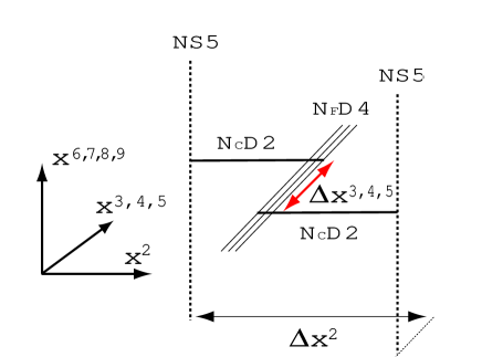
Figure 3: The T-dualized brane configuration for massless hypermultiplets. The triplet of the FI-parameters correspond to separations $\Delta x^{3,4,5}$ of the D$2$-branes along the D$4$-branes. Separation $\Delta x^{2}$ of the two NS$5$-branes along the $x^{2}$-coordinate is proportional to the gauge coupling constant squared on the effective theory on the D$2$-branes.

Here the positions of the two NS$5$-branes have the following physical meanings. The distance $\Delta x^{2}$ between the NS$5$-branes along the $x^{2}$-coordinate is proportional to inverse of the square of the gauge coupling constant $g$ in the effective gauge theory on the D($p+1$)-branes:

$${1\over g^{2}}=|\Delta x^{2}|\tau_{p+1}\,l_{s}^{4}={|\Delta x^{2}|\over g_{s}l_{s}^{p-2}}$$ (3.7)

with $g_{s}$ and $l_{s}=\sqrt{\alpha^{\prime}}$ the string coupling constant and the string length in the T-dualized type II sting theory, respectively. The triplet of the FI-parameters correspond to the distance between the two NS$5$-branes in the coordinates $x^{3}$, $x^{4}$ and $x^{5}$:

$$c^{a}=\frac{1}{g_{s}l_{s}^{p}}(\Delta x^{3},\Delta x^{4},\Delta x^{5}).$$ (3.8)

In the limit of vanishing FI-parameters, there can appear non-baryonic Higgs branches realized by D($p+1$)-branes stretched between two NS$5$-branes directly [22, 24, 25]. Due to non-vanishing FI-parameters, these D($p+1$)-branes cannot be supersymmetric without total gauge symmetry breaking and therefore non-baryonic branches are prohibited.

Strings connecting $N_{\rm C}$ D$(p+1)$-branes and $N_{\rm F}$ D$(p+3)$-branes give the $N_{\rm C}\times N_{\rm F}$ matrix of hypermultiplets. The effective gauge theory on the world-volume of D$p$-branes is insensitive to the positions of the $N_{\rm F}$ D$(p+3)$-branes in the $x^{2}$-coordinate, and so they are arbitrary. The moduli space of the vacua ${\cal M}^{M=0}_{\rm vacua}$ of the theory is identical to the one $T^{*}G_{N_{\rm F},N_{\rm C}}$ in Eq. (3.3) before taking the T-duality. We can count the dimension of ${\cal M}^{M=0}_{\rm vacua}$ easily, if the configuration is viewed from the $x^{6,7,8,9}$-directions as in Fig. 4.

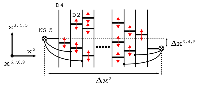
Figure 4: The moduli space for vacua. Its dimension can be counted as the D$2$-brane degree of freedom in the $x^{3,4,5}$-positions and the position on $S^{1}$ in the M-theory. The s-rule plays a crucial role for this counting.

The D($p+1$)-branes stretched between D($p+3$)-branes can move freely in the $x^{3},x^{4},x^{5}$-coordinates. Here we have a very important rule called the s-rule (see for review and references in [27]) which requires that at most one D$(p+1)$ can be stretched between a D$(p+3)$ brane and a NS$5$-brane. Thanks to this rule some D($p+1$)-brane cannot move in the $x^{3},x^{4},x^{5}$-coordinates because they are connected to one of NS$5$-branes directly, and therefore the dimension of the moduli space of vacua can be calculated by counting the freedom of the D($p+1$)-branes as [24]

$$\dim{\cal M}^{M=0}_{\rm vacua} = 4\left[2\sum_{k=1}^{N_{\rm C}}k+N_{\rm C}(N_{\rm F}-1-2N_{\rm C})\right]$$ (3.9)

$$= 4N_{\rm C}(N_{\rm F}-N_{\rm C})=\dim T^{*}G_{N_{\rm F},N_{\rm C}}$$

which coincides again with the field theoretical result (2.3). The factor four comes from the freedom of the D($p+1$)-brane endpoint positions on the world-volume $x^{3}$, $x^{4}$ and $x^{5}$ of the D($p+3$)-branes and position on $S^{1}$ of the eleventh direction when this system is promoted from the type IIA theory to the M-theory.

If we did not divide ${\bf C}^{2}$ by ${\bf Z}_{2}$ there would be no NS$5$-branes and therefore the s-rule does not play any roles in its T-dual picture. Then the moduli space dimension becomes $4N_{\rm C}N_{\rm F}$, and the difference $4N_{\rm C}^{2}$ with the dimension (3.9) is supplied from adjoint hypermultiplets which are projected out by ${\bf Z}_{2}$ in our case. Therefore the s-rule was essential to get correct results for our ${\bf Z}_{2}$ case.

3.2 Massive Hypermultiplets

For the presence of domain walls in the theory we need to give mass differences to the hypermultiplets. We consider the case of non-degenerate masses and briefly discuss the partially degenerate masses in Sec. 5. In the T-dual picture, masses for hypermultiplets are obtained by sliding D$(p+3)$-branes along the NS$5$-brane world-volume as shown in Fig. 5.

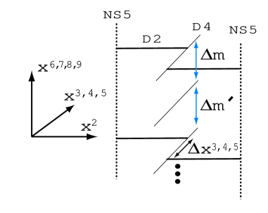
Figure 5: The brane configuration for massive hypermultiplets. Hypermultiplets coming from strings stretched between D$2$- and D$4$-branes become massive by placing D$4$-branes with distances in the $x^{6,7,8,9}$-coordinates. $\Delta m$ and $\Delta m^{\prime}$ denote mass differences for the hypermultiplets. The relation with coordinates is $\Delta\vec{m}=l_{s}^{-2}(\Delta x^{6},\Delta x^{7},\Delta x^{8},\Delta x^{9})$.

Note that the freedom of sliding and therefore the number of mass parameters for one hypermultiplet depend on the dimension $p$. There exist four degrees of freedom in the case of $p=1$,

$$\Delta\vec{m}=\frac{1}{l_{s}^{2}}(\Delta x^{6},\Delta x^{7},\Delta x^{8},\Delta x^{9}).$$ (3.10)

However we simply exploit one freedom for instance the $x^{6}$-direction in the brane configuration in this paper, and therefore hypermultiplets have real masses with this choice. The whole discussion in this paper holds in any dimensions $p=1,2,3,4$.

We consider the vacua of this theory. Again the s-rule plays an important role: at most one D$(p+1)$-brane can stretch between a D$(p+3)$-brane and a NS$5$-brane. Therefore vacua are discrete and isolated, and the number of them is ${}_{N_{\rm F}}C_{N_{\rm C}}$ recovering the field theoretical result (2.6). The case of hypermultiplets with degenerate masses can be considered by letting positions of some D$(p+3)$-branes to coincide. There appear more massless degrees of freedom from strings stretched between D$(p+1)$-branes and D$(p+3)$-branes resulting in continuous vacua as in the massless case.

Next let us consider the original brane configuration before the T-dualization. Masses of hypermultiplets correspond to the positions of the D$(p+4)$-branes. In the case of $p=1$, the quartets of masses (3.10) are given by the D($p+4$)-brane positions in the $x^{6,7,8,9}$-directions as seen in Fig. 6. We assume real masses for hypermultiplets by placing D($p+4$)-branes parallel along the $x^{6}$-direction.

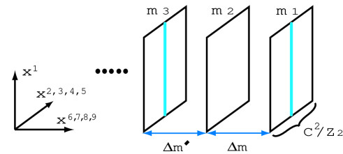
Figure 6: The brane configuration for massive hypermultiplets before the T-dualization. Hypermultiplets coming from strings stretched between D$1$- and D$5$-branes become massive by placing D$5$-branes with distances in the $x^{6,7,8,9}$-coordinates.

The D$(p+4)$-branes are ordered by the single coordinate $x^{6}$ for real masses. We label D$(p+4)$-branes by $A=1,\cdots,N_{\rm F}$ such that a larger $x^{6}$ position corresponds to a smaller $A$. To be consistent with the s-rule in the T-dual picture, we find that at most one D$p$-brane can be absorbed into the ${\bf Z}_{2}$ fixed point of one D$(p+4)$-brane. We thus have “the exclusion principle of D$p$-branes”. It will play an important role to consider domain wall dynamics in the next section. From this exclusion principle the discrete vacua are labeled by a set of the flavor indices $A_{r}$ ($r=1,\cdots,N_{\rm C}$) corresponding to the $A_{r}$-th D$(p+4)$-brane into which the $r$-th D$p$-brane is absorbed. Such a configuration can be read from the vacuum expectation values for hypermultiplets

$$H^{1\dagger}H^{1}=c\,{\rm diag}.(0,\cdots,1,0,\cdots,1,0,*,\cdots,*),$$ (3.11)

$$\hskip 119.50157ptA_{1}\hskip 31.29802ptA_{2}$$

where positions of the D$p$-branes can be read from the elements 1. We label such a vacuum by $\langle A_{1},\cdots,A_{N_{\rm C}}\rangle$ as in Eq. (2.5). Again, the number of vacua can be calculated as ${}_{N_{\rm F}}C_{N_{\rm C}}$ recovering the field theoretical result (2.6).

3.3 Duality

In this subsection we discuss a duality between theories with the gauge groups $U(N_{\rm C})$ and $U(\tilde{N}_{\rm C})$ and the same number of hypermultiplets, where the dual gauge group is defined by $\tilde{N}_{\rm C}\equiv N_{\rm F}-N_{\rm C}$. When a NS$5$-brane moves across a D($p+3$)-brane, a D($p+1$)-brane is created (annihilated) between these branes (see Fig. 7). This phenomenon is known as the Hanany-Witten effect [22, 26].

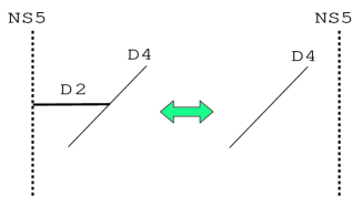
Figure 7: The Hanany-Witten effect. A D$2$-brane is created (annihilated) when NS$5$-brane moves across a D$4$-brane.

Let us exchange the positions of two NS$5$-branes both across the D($p+3$)-branes in the brane configuration in Fig. 5 with noting the Hanany-Witten effect. Then we obtain the vacuum configuration for the dual gauge theory on the D($p+1$)-branes with $U(\tilde{N}_{\rm C})$ gauge group with $N_{\rm F}$ fundamental hypermultiplets (see Fig. 8).

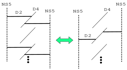
Figure 8: The duality between $N_{\rm C}$ and $\tilde{N}_{\rm C}=N_{\rm F}-N_{\rm C}$ in the brane configuration.

From this figure we can see that the sign of the FI-parameter is flipped under this duality. As a result roles of $H^{1}$ and $H^{2}$ in hypermultiplets are exchanged

$$(H^{1},H^{2},c)\leftrightarrow(\tilde{H}^{2},\tilde{H}^{1},\tilde{c}=-c)$$ (3.12)

with $\tilde{H}^{1}$ and $\tilde{H}^{2}$ denoting a doublet of $\tilde{N}_{\rm C}\times N_{\rm F}$ matrices of hypermultiplets in the dual theory. For instance $\tilde{H}^{2}$ ($H^{1}$) and $\tilde{H}^{1}$ ($H^{2}$) parametrize the base and cotangent space of the vacuum manifold $T^{*}G_{N_{\rm F},\tilde{N}_{\rm C}}$ ($T^{*}G_{N_{\rm F},N_{\rm C}}$), respectively, after (before) taking the duality.

In the spirit of ${\cal N}=1$ Seiberg duality the above duality merely means the possibility of continuous deformation of parameters of the theory. Namely there is no phase boundary between two theories resulting in the identical low-energy effective theory. On the other hand Eq. (3.7) implies that the distance $\Delta x^{2}$ of the two NS$5$-branes in the $x^{2}$-coordinate is proportional to the inverse of the gauge coupling constant squared in the gauge theories on the D($p+1$)-branes for both brane configurations. Therefore this duality becomes exact in the limit of $\Delta x^{2}\to\pm 0$. In fact these gauge theories reduce to nonlinear sigma models on $T^{*}G_{N_{\rm F},N_{\rm C}}$ in this limit, and the duality $N_{\rm C}\leftrightarrow\tilde{N}_{\rm C}$ becomes exact (3.13).

In the original brane picture for the vacua in Fig. 6 before taking the T-duality the Hanany-Witten effect can be understood as a rule to exchange existence and non-existence of the D$p$-branes at every D($p+4$)-brane although creation/annihilation is not so clear (see Fig. 9).

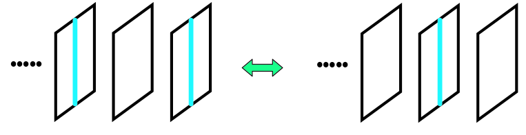
Figure 9: The duality between $N_{\rm C}$ and $N_{\rm F}-N_{\rm C}$ in the brane configuration before the T-dualization.

In the strong coupling limit, the duality between theories with $N_{\rm C}$ and $\tilde{N}_{\rm C}=N_{\rm F}-N_{\rm C}$ holds as can be seen in Eq. (2.3). Since we know that only fields parameterizing the base space of the target space participate in constructing walls, we set $H^{2}=0$ and $\tilde{H}^{1}=0$. Then the duality is determined by [see Eq. (D.5) in [14]]

$$H^{1\dagger}H^{1}+\tilde{H}^{2\dagger}\tilde{H}^{2}=c{\bf 1}_{N_{\rm F}},$$ (3.13)

where $H^{1}$ is for $U(N_{\rm C})$ gauge theory and $\tilde{H}^{2}$ is that in $U(\tilde{N}_{\rm C})$ gauge theory. This equation implies the relation between $H^{1}$ and $\tilde{H}^{2}$ [see Eq. (D.4) in [14]]

$$H^{1}\tilde{H}^{2}{}^{\dagger}=0.$$ (3.14)

The vacuum expectation values of hypermultiplets in the vacuum configuration after taking a duality are found from Eqs. (3.11) and (3.13) as

$$\tilde{H}^{2\dagger}\tilde{H}^{2}=c\,{\rm diag}.(1,\cdots,0,1,\cdots,0,1,*,\cdots,*).$$ (3.15)

$$\hskip 119.50157ptA_{1}\hskip 31.29802ptA_{2}$$

The elements 1 and 0 in Eqs. (3.11) and this equation are exchanged under the duality, indicating Fig. 9. In the next section we will see that the Hanany-Witten effect is generalized to kinky configurations.

4 Non-Abelian Walls as Multiple Kinky D-branes

4.1 Multiple Kinky D-branes

As shown above the effective theory on the fractional D$p$-branes is the SUSY $U(N_{\rm C})$ gauge theory with massive $N_{\rm F}$ hypermultiplets and the FI-term. Since the adjoint scalar field $\Sigma$ represents transverse fluctuations of D$p$-branes, the diagonal components of (the vacuum expectation value of) $\Sigma$, in the gauge of diagonal $\Sigma$, can be identified as the positions of $N_{\rm C}$ D$p$-branes along the $x^{6}$-coordinate. In that gauge $N_{\rm C}$ diagonal components of $\Sigma$ for a wall solution are plotted as functions $x^{6}=\Sigma_{rr}(x^{1})$ in Fig. 10. They represent multiple kinky D$p$-branes curved in the ($x^{1}$,$x^{6}$)-plane and these curves are determined by the BPS equations (2.7).

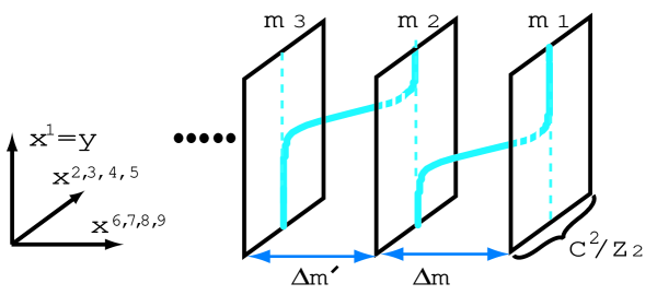
Figure 10: Multiple kinky fractional D-branes.

To be more precise, all D$p$-branes are absorbed into some $N_{\rm C}$ D$(p+4)$-branes in the limit $y=x^{1}\to+\infty$. The configuration tends to a vacuum state $\langle A_{1},\cdots,A_{N_{\rm C}}\rangle$ in this limit where we have labeled the $r$-th D$p$-brane counted from the right of Fig. 10 by $A_{r}$. On the other hand, in the opposite limit $y\to-\infty$, they approach another vacuum configuration labeled by $\langle B_{1},\cdots,B_{N_{\rm C}}\rangle$. The $N_{\rm C}$ D$p$-branes exhibit kinks somewhere in the $y$-coordinate as illustrated in Fig. 11.

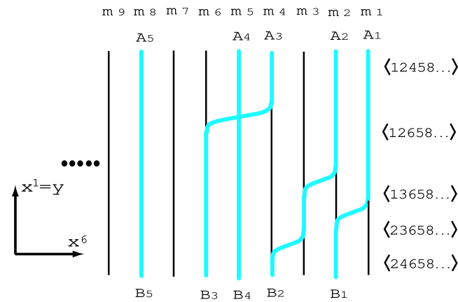
Figure 11: Multiple non-Abelian walls as kinky D-branes. An example of the $N_{\rm C}$ kinky D$p$-branes interpolating between the vacua $\langle A_{1},\cdots,A_{N_{\rm C}}\rangle$ and $\langle B_{1},\cdots,B_{N_{\rm C}}\rangle$ is displayed. Intermediate vacua between two adjacent walls plotted on the right of the figure can be easily read from this kinky brane configuration.

Here we labeled $B_{r}$ such that the $A_{r}$-th brane at $y\to+\infty$ goes to the $B_{r}$-th brane at $y\to-\infty$. The labels $r$ for the vacua are now understood to be given for the $r$-th D$p$-brane. Hence a set of $B_{r}$ does not have to be ordered. If we separate adjacent walls far enough the configuration between these walls approach a vacuum. The brane configurations are very useful to figure out such a vacuum as illustrated in Fig. 11.

It is sometimes troublesome to take a gauge of diagonal $\Sigma$. Without taking that gauge the positions of the D$p$-branes in the $x^{6}$-coordinate can be described in a gauge invariant way by solutions $\lambda$ of the eigenvalue equation

$$0=\det(\lambda{\bf 1}_{N_{\rm C}}-\Sigma)=\det\left(\lambda-{1\over 2}\Omega^{-1}\partial_{y}\Omega\right)\;.$$ (4.1)

We now calculate the wall tension (2.8) using the brane configurations a) before and b), c), d) after taking T-duality using figures a) and b), c), d) of Fig. 12, respectively.

a) The orbifold singularity in ${\bf C}^{2}/{\bf Z}_{2}$ is blown up by $S^{2}\simeq{\bf C}P^{1}$ and ${\bf C}^{2}/{\bf Z}_{2}$ becomes the $A_{1}$ gravitational instanton, the Eguchi-Hanson space $T^{*}{\bf C}P^{1}$. Fractional D$p$-branes are D($p+2$)-branes two of whose spatial dimensions are wrapped around the 2-cycle $S^{2}$ with the area proportional to the FI-parameter $c$ as in Eq. (3.4). Since fractional D$p$-branes for the vacuum state in Fig. 6 are actually D($p+2$)-branes with size $\sqrt{c}$ of this $S^{2}$, the tension of a fractional D$p$-brane is proportional to the area of the fractional D$p$-brane ($\sim c\Delta x^{1}$) which diverges because of the world-volume extending to the $x^{1}$-coordinate. Kinky fractional D$p$-branes in Fig. 10 also wrap around the $S^{2}$ with the area $c$ as illustrated in Fig. 12-a).

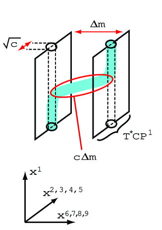
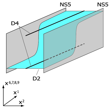
a)		b)
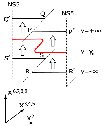
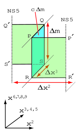
c)		d)

Figure 12: Calculating the wall tension in the brane configuration before a) and after b), c), d) taking T-duality. a) The wall tension is given by the tension of the fractional D$p$-branes subtracted by the one for the D$p$-branes in the vacuum state. b) The wall profile (kinky D($p+1$)-branes) in the T-dualized brane configuration with suppressing the directions $x^{3,4,5}$ for the FI term. c) The wall profile with suppressing the direction $x^{1}=y$ of the co-dimension of the wall. The D($p+1$)-branes stay at the segments RR^′ and S^′S for $y\to-\infty$. They move up around $y=y_{0}$ apart from the lower D($p+3$)-brane. Here they have to bend to the $x^{3}$ direction to be connected with each other. Finally they stay at the segments PR^′ and Q^′Q for $y\to+\infty$. d) The movement of the D($p+1$)-brane depending on $y$ is drawn in the same figure. The wall tension is given by at the square PQSR. Tensions proportional to the squares PP^′R^′R and QQ^′S^′S are contributions from vacua.

The tension of a kinky D$p$-brane interpolating between adjacent D($p+4$)-branes with the distance $\Delta x^{6}\sim\Delta m$ increases from the one for a vacuum state by the finite amount coming from the area of the kinky region of the D$p$-brane. That amount of the tension contributed from a kink can be calculated by subtracting the tension of the fractional D$p$-brane for vacuum states from that of the kinky configuration, to give

$$\tau_{p+2}[{\rm Area}\,(\mbox{kinky frac. D$p$})-{\rm Area}\,(\mbox{vacuum frac. D$p$})]$$

$$=\frac{1}{g_{s}l_{s}^{p+3}}[A(\Delta x^{1}+\Delta x^{6})-A\Delta x^{1}]=c\,\Delta m$$ (4.2)

with $\tau_{p+2}=1/g_{s}l_{s}^{p+3}$ and $\Delta x^{6}=l_{s}^{2}\Delta m$ in Eq. (3.10). The last equality holds provided that the $g_{s}$ dependence of the area $A$ of $S^{2}$ in Eq. (3.4) is given by

$$A=cg_{s}l_{s}^{p+1}={c\over\tau_{p}}.$$ (4.3)

For multiple fractional D$p$-branes exhibiting multiple kinks, the sum of the kink contributions to the tension of the kinky D$p$-branes can be obtained as

$$\tau_{p+2}\sum_{r=1}^{N_{\rm C}}[{\rm Area}\,(\mbox{$r$-th kinky frac. D$p$})-{\rm Area}\,(\mbox{$r$-th vacuum frac. D$p$})]=c\sum_{r=1}^{N_{\rm C}}(m_{A_{r}}-m_{B_{r}}).$$ (4.4)

Therefore the tension of the fractional D$p$-branes in our brane configuration correctly reproduces the tension formula (2.8) of walls.

b), c), d) The wall tension (2.8) can also be calculated in the brane configuration after taking T-duality. The directions corresponding to the FI-term are not displayed in Fig. 12-b). This figure is not useful to calculate the wall tension. Instead, we consider Fig. 12-c) and d) where the co-dimension $y=x^{1}$ of walls is not displayed. The two D($p+1$)-branes ending on the lower D($p+3$)-brane along the segment RS at $y\to-\infty$ are expressed by the segments RR^′ and SS^′. They go to the D($p+1$)-branes, ending on the upper D($p+3$)-brane along PQ, expressed by the segments PP^′ and QQ^′ at $y\to+\infty$, respectively. At intermediate $y\sim y_{0}$ with $y_{0}$ the wall position, the two D($p+1$)-branes cannot end on any D($p+3$)-branes and therefore they have to bend to the $x^{3}$-direction to be connected with each other as drawn in Fig. 12-c). By drawing the configurations at all $y$ in the same figure, we have the configuration illustrated in Fig. 12-d). We now calculate the wall tension in Fig. 12-d). The tension of the D($p+1$)-brane is given by the sum of three pieces, Area (PQSR), Area (PP^′R^′R) and Area (QQ^′S^′S). The contribution from the last two terms

$$\tau_{p+1}[\mbox{Area (PP${}^{\prime}$R${}^{\prime}$R)}+\mbox{Area (QQ${}^{\prime}$S${}^{\prime}$S)}]=\tau_{p+1}\Delta x^{2}\Delta x^{6}={\Delta m\over g^{2}l_{s}^{2}}$$ (4.5)

diverges in the limit $l_{s}\to 0$, where we have used Eqs. (3.7) and (3.10). However this is contribution from the vacuum energy and we have to subtract it to obtain the wall tension. This fact can be understood by taking the limit $\Delta x^{3}\sim c\to 0$. In this limit the two D($p+1$)-branes are connected with each other to become one D($p+1$)-brane directly stretched between the two NS$5$-branes at all $y$. The D($p+1$)-brane at each $y$ corresponds to a vacuum in the baryonic branch. Therefore the D($p+1$)-brane tension contributed from the kink is calculated from Eqs. (3.8) and (3.10), to yield

$$\tau_{p+1}\times{\rm Area(PQSR)}=\tau_{p+1}\Delta x^{3}\Delta x^{6}=c\Delta m$$ (4.6)

with $\tau_{p+1}=1/g_{s}l_{s}^{p+2}$. We thus have reproduced the wall tension (2.8) in this brane configuration.

A brane configuration for a recently found monopole in the Higgs phase (a confined monopole) [18, 16] has been given by Hanany and Tong [5] (see also [20]). It looks very similar with our brane configuration for walls in Fig. 12-d). We discuss this issue in Sec. 5.

4.2 Duality for Walls and Extension of the Hanany-Witten Effect

In the strong gauge coupling limit the duality between the theories with the gauge groups $U(N_{\rm C})$ and $U(\tilde{N}_{\rm C})$ with the same number $N_{\rm F}$ of hypermultiplets holds exactly also for wall solutions as shown in [14] by a field theoretical analysis. Let us now consider the implication of this field theoretical result of duality of the non-Abelian walls to the Hanany-Witten effect in the brane configuration. Since the gauge coupling constant on the D($p+1$)-branes in the T-dualized configuration is given in Eq. (3.7), the strong gauge coupling limit corresponds to the positions of the two NS$5$-branes with $\Delta x^{2}\to\pm 0$ as stated above. The original Hanany-Witten effect explains the duality of the vacua at both infinities $y\to\pm\infty$ when the positions of the two NS$5$-branes in the $x^{2}$-coordinate are exchanged. It is, however, difficult to visualize what happens for kinky configurations in the finite region of $y$.

Therefore we consider the original brane configuration before the T-dualization. Then the result in [14] implies that this duality $N_{\rm C}\leftrightarrow\tilde{N}_{\rm C}$ in the strong gauge coupling limit can be drawn in Fig. 13.

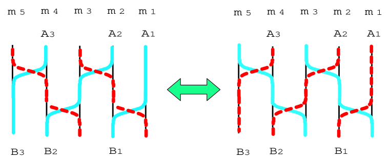
Figure 13: Duality between wall configurations in theories with gauge groups $U(N_{\rm C})$ and $U(N_{\rm F}-N_{\rm C})$. Examples of wall configurations in the theory with $N_{\rm F}=5$ and $N_{\rm C}=3$ and its dual theory with $N_{\rm F}=5$ and $\tilde{N}_{\rm C}=2$ are illustrated. The broken curves are wall configurations in the dual theory in both figures. The dual wall configurations curve oppositely due to the flip of the sign of the FI-parameter under the duality.

Here wall configurations are given by $H^{1}$ with $H^{2}=0$ ($\tilde{H}^{2}$ with $\tilde{H}^{1}=0$) for the theory with $U(N_{\rm C})$ [$U(\tilde{N}_{\rm C})$], since flip of the sign of the FI-parameter occurs and the roles of $H^{1}$ and $H^{2}$ are exchanged in both configurations as explained in Eq. (3.12). We define the moduli matrix for the dual theory generating $\tilde{H}^{2}$ by $\tilde{H}_{0}$. Here Eqs. (2.9) and (2.10) with tilde on all quantities hold for the dual theory and we have $\tilde{H}_{0}^{1}=0$, $\tilde{H}_{0}^{2}=\tilde{H}_{0}$ for its moduli matrices instead of Eq. (2.11). Then the relation (3.14) between the hypermultiplets $H^{1}$ and $\tilde{H}^{2}$ in both theories implies the relation between the moduli matrices $H_{0}$ and $\tilde{H}_{0}$, given by [see Eq. (D.14) in [14]]

$$H_{0}\tilde{H}_{0}{}^{\dagger}=0.$$ (4.7)

For a given moduli matrix $H_{0}$ in the original theory, the form of the moduli matrix $\tilde{H}_{0}$ for the dual theory is determined up to the world-volume symmetry (2.14) from this equation.

Wall solutions in dual theories can be mapped to each other in the strong gauge coupling limit as stated above, but they are not identical for finite gauge coupling in general. Namely, wall solutions under exact duality for the two NS$5$-branes with $\Delta x^{2}\to\pm 0$ are deformed for finite gauge coupling with $\Delta x^{2}\neq 0$ in different ways in both configurations. Although we did not obtain exact wall solutions for finite gauge coupling, dual configurations can be determined without loss of exactness by the same relation (4.7) between the moduli matrices for both configurations. Although the relation (4.7) was originally found in the strong gauge coupling limit we define the dual configuration for finite gauge coupling by that equation. We thus conclude that the Hanany-Witten effect should be extended to kinky D-brane configuration.

4.3 Impenetrable Walls and Extension of the S-rule/ Reconnection of D-branes

We show that a lot of interesting phenomena of non-Abelian walls found in field theory [14] can be explained very easily by means of the brane configurations. A double wall configuration for $N_{\rm C}=1$ and $N_{\rm F}=3$ is shown in Fig. 14-a). These two walls are labeled by $\langle 1\leftarrow 2\rangle$ and $\langle 2\leftarrow 3\rangle$ using the vacuum labels at $y\to+\infty$ and $y\to-\infty$. Positions of these walls cannot be exchanged (they are called impenetrable) because the configuration approaches a single wall $\langle 1\leftarrow 3\rangle$ when they are compressed [Fig. 14-b)].

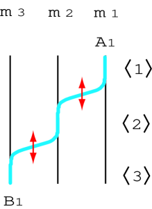
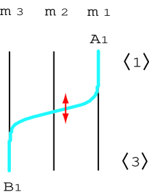
a)	b)

Figure 14: Compressing two walls (a self-compressed brane).

The moduli matrices for these configurations before and after compression are

$$H_{0}=\sqrt{c}\,(1,e^{r},e^{s}),$$ (4.8)

$$H_{0}=\sqrt{c}\,(1,0,e^{s})\;,$$ (4.9)

respectively, with $e^{r}\in{\bf C}$ and $e^{s}\in{\bf C}^{*}$. In the strong gauge coupling limit, the wall solution for Fig. 14-a) can be obtained by substituting the moduli matrix (4.8) to Eq. (2.25) and by using Eqs. (2.9) and (2.12), to yield

$$\Sigma={m_{1}e^{2m_{1}y}+m_{2}e^{2m_{2}y+2{\rm Re}(r)}+m_{3}e^{2m_{3}y+2{\rm Re}(s)}\over e^{2m_{1}y}+e^{2m_{2}y+2{\rm Re}(r)}+e^{2m_{3}y+2{\rm Re}(s)}},\hskip 14.22636ptW_{y}=0.$$ (4.10)

The positions of kinks can be roughly estimated as (see Appendix A in [14])

$$y_{1}={{\rm Re}(r)\over m_{1}-m_{2}},\hskip 14.22636pty_{2}={{\rm Re}(s-r)\over m_{2}-m_{3}}\;,$$ (4.11)

which are valid when these two walls are well separated. The wall configuration in Fig. 14-b) is obtained in the limit of ${\rm Re}(r)\to-\infty$ with the center of position $s$ of two walls fixed. [It is also obtained from the moduli matrix (4.9).] There the interpretation of parameters in Eq. (4.11) as the positions becomes meaningless. We call this compressed wall a level-1 compressed wall, where the “level” of compression have been defined by the number of zero components between $1$ and the non-zero element.

In the same way positions of walls made by the same D$p$-brane cannot commute and they are impenetrable. So the Abelian walls in the $U(1)$ gauge theory are all impenetrable. A level-$l$ compressed wall in $U(N_{\rm C})$ gauge theory is generated by a moduli matrix in the form of

$$H_{0}=\sqrt{c}\,\left(\begin{array}[]{ccc}&\cdots&\\ \cdots&1\underbrace{0\cdots 0}_{l}&e^{r}\cdots\\ &\cdots&\end{array}\right)\;.$$ (4.15)

We can obtain this configuration by compressing elementary walls $l$ times.

The dual theory of the above example with $N_{\rm C}\leftrightarrow\tilde{N}_{\rm C}$ is the theory with $N_{\rm C}=2$ and $N_{\rm F}=3$. The double wall configuration in this model was discussed in detail in Sec. 4 in Ref. [14]. The dual brane configuration of Fig. 14 is shown in Fig. 15 (with $y\to-y$).

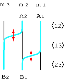
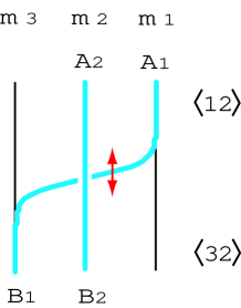
a)	b)

Figure 15: Compressing walls understood by a reconnection of two D$p$-branes (crossing brane). These configurations are dual to Fig. 14-a) and -b), respectively, with $y\to-y$. However physics occurring here is more interesting.

In this case the process of compressing two walls is very interesting. A double wall configuration in Fig. 15-a) can be labeled as $\langle 12\leftarrow 23\rangle$. The moduli matrix for that configuration is given by

$$H_{0}=\sqrt{c}\,\left(\begin{array}[]{ccc}1&e^{r}&0\\ 0&1&e^{s}\end{array}\right)\;,$$ (4.18)

with $e^{r},e^{s}\in{\bf C}^{*}$. [Also this can be obtained from the moduli matrix (4.8) using the relation (4.7) with relabeling $\tilde{H}_{0}$ by $H_{0}$.] The wall solution is obtained in Eq. (4.17) of [14] as

$$\Sigma^{0}=m{e^{2my}-e^{-2my}\over e^{2my}+e^{-2my}+e^{mR}}\sim\left\{\begin{array}[]{cc}\pm m,&2|y|\gg R,\quad y=\pm|y|\\ 0,&2|y|\ll R\end{array}\right.$$ (4.21)

$$|\Sigma^{3}|=2m{\sqrt{(\cosh({2my})+e^{mR})^{2}-1}\over e^{2my}+e^{-2my}+e^{mR}}\sim\left\{\begin{array}[]{cc}m,&2|y|\gg R\\ 2m,&2|y|\ll R\end{array}\right.,$$ (4.24)

$$\sqrt{(W^{1}_{y})^{2}+(W^{2}_{y})^{2}}={\sqrt{4m^{2}e^{mR}(e^{2my}+e^{-2my}+e^{mR})}\over(\cosh({2my})+e^{mR})^{2}-1},\;$$

$$\Sigma^{1}=\Sigma^{2}=W^{3}_{y}=0,$$ (4.25)

where we have set $M={\rm diag.}(m,\,0,\,-m)$ and $(s,r)=(mR/2+i\theta/2,-mR/2-i\theta/2)$ for simplicity. The configuration approaches the vacuum $\langle 13\rangle$ between these two walls. Therefore this double wall configuration is approximately made of two walls $\langle 12\leftarrow 13\rangle$ and $\langle 13\leftarrow 23\rangle$.

We now discuss the limit of compressing these two walls in Fig. 15-b) in the level of the moduli matrix (4.18). (This limit for the solution (4.25) in strong coupling will be discussed in (4.37), below.) To take this limit we first need to transform $H_{0}$ by a world-volume symmetry (2.14) as

$$H_{0}\to H_{0}^{\prime}=VH_{0}=\sqrt{c}\,\left(\begin{array}[]{ccc}1&0&-e^{r+s}\\ 0&1&e^{s}\end{array}\right)\,,\hskip 14.22636ptV=\left(\begin{array}[]{cc}1&-e^{r}\\ 0&1\end{array}\right)\,.$$ (4.30)

Taking the limit

$$e^{s}\to 0,\hskip 14.22636pte^{r}\to\infty$$ (4.31)

with keeping $-e^{r+s}(\equiv e^{t}\in{\bf C}^{*})$ fixed, we obtain the moduli matrix

$$H_{0}=\sqrt{c}\,\left(\begin{array}[]{ccc}1&0&e^{t}\\ 0&1&0\end{array}\right)\,.$$ (4.34)

We express this moduli matrix by $\langle 12\leftarrow 32\rangle$. In the strong gauge coupling limit the wall solutions for this moduli matrix can be calculated, to yield

$$\Sigma=\left(\begin{array}[]{cc}\frac{m_{1}e^{2m_{1}(y-y_{1})}+m_{3}e^{2m_{3}(y-y_{1})}}{e^{2m_{1}(y-y_{1})}+e^{2m_{3}(y-y_{1})}}&0\\ 0&m_{2}\end{array}\right),\hskip 14.22636ptW_{y}=0,\hskip 14.22636pty_{1}={{\rm Re}(t)\over m_{1}-m_{3}}$$ (4.37)

where $y_{1}$ denotes the position of the compressed wall. This gives a compressed kinky configuration in Fig. 15-b). The configuration is made of the D$p$-brane interpolating between the first and the third D($p+4$)-branes and the one staying at the second D($p+4$)-brane representing a vacuum state [see Fig. 15-b)]. They correspond to the first and the second rows in the matrix (4.34), respectively.

This phenomenon can be understood by recalling the s-rule as the exclusion principle for D$p$-branes which states that two D$p$-branes cannot be placed at the same D($p+4$)-brane. Although this s-rule was originally suggested for vacuum states, we find from this example that the s-rule for vacuum states is extended to the case of kinky D-brane configurations. We may call it the extended s-rule.

Moreover this phenomenon can be understood in terms of the reconnection (recombination) of D-branes. A reconnection process was analyzed in Ref. [37] in the gauge theory on D-branes. There a reconnection of straightly intersecting D-branes was examined. In the case of an intersection of a $(p,q)$-string and a D-string with a particular angle determined by $p$ and $q$, the configuration is BPS. The reconnection occurs by off-diagonal elements of gauge fields as a marginal deformation of a moduli parameter as shown by K. Hashimoto and W. Taylor in [37]. Our model gives a similar but complicated example of the reconnection of two D$p$-branes in a kinky configuration, which still can be analyzed in the gauge theory on D-branes. In the case of [37] a singular gauge transformation is needed to connect the left and the right sides of the configuration in the limit when the reconnection occurs. In fact, completely the same thing occurs in our case also. The world-volume transformation $V$ in Eq. (4.30) diverges in the limit (4.31) of the reconnection. Correspondingly a singular gauge transformation is needed in that limit as seen as follows. We take $\theta=0$ without loss of generality. With a gauge choice $\Sigma^{1}=\Sigma^{2}=W^{3}_{y}=0$, we find that an off-diagonal component of the gauge field

$$W^{1}_{y}={\sqrt{4m^{2}e^{mR}(e^{2my}+e^{-2my}+e^{mR})}\over(\cosh({2my})+e^{mR})^{2}-1},\;\hskip 14.22636ptW^{2}_{y}=0$$ (4.38)

exists before the reconnection. This off-diagonal component $W^{1}_{y}$ can be regarded as a moduli parameter of a marginal deformation instead of $R$ because it is a function of $R$. This tends to the delta function, $W^{1}_{y}\to\pi\delta(y)$, in the limit of the reconnection ($R\to-\infty$). To eliminate it we need a singular gauge transformation $W_{y}^{1}\rightarrow W_{y}^{1^{\prime}}=W_{y}^{1}+\partial_{y}\Lambda(y)=0$ with a gauge parameter of the step function, $\Lambda(y)=\pi\Theta(-y)$. The wall solution becomes the one in Eq. (4.37) [with $M={\rm diag.}(m,\,0,\,-m)$ and $(s,r)=(mR/2+i\theta/2,-mR/2-i\theta/2)$]. Therefore we conclude that the reconnection process in this model is the same as the one of the BPS case in [37]. This observation suggests that the extended s-rule can be understood in terms of the reconnection process.

We make a brief comment here. The moduli matrix (4.34) is one called $U(1)$-factorisable as defined in Sec. 3.7 in [14]. In the $U(1)$-factorisable cases the BPS equations reduce to a set of those of the $U(1)$ gauge theory, and therefore they can be solved if those in the $U(1)$ gauge theory are solved. The compressed wall solution, generated by the moduli matrix (4.34), in the theory with $N_{\rm C}=2$ and $N_{\rm F}=3$ for the finite gauge coupling coincides with the single wall solution, generated by the moduli matrix (4.9), in the dual theory with $N_{\rm C}=1$ and $N_{\rm F}=3$ for the same gauge coupling. Namely the kinky D$p$-branes in Fig. 14-b) and Fig. 15-b) coincide with each other even for finite gauge coupling, and the vacuum D$p$-brane in the latter does not contribute to wall configurations. Therefore both configurations before and after taking the duality coincide with each other for the same distance between the two NS$5$-branes [because of the relation (3.7)], except for the vacuum D$p$-brane in the middle D($p+4$)-brane. Thus the extended Hanany-Witten effect happens to give an exact duality in this case.

This example shows that existence of a compressed wall or a reconnected wall reduces the number of the moduli parameters in the same topological sector. In other words, the full dimensionality of the topological sector can be counted only when the configuration is generic, namely with no compressed walls nor reconnected branes, as will be discussed in the subsection 4.5.

4.4 Penetrable Walls

All walls are impenetrable in the $U(1)$ gauge theory as stated in the last subsection. A characteristic feature of non-Abelian walls is that there also exist pairs of walls whose positions can be exchanged under a marginal deformation by changing moduli parameters slowly. They are called penetrable walls. This can occur because the size of the matrix $\Sigma$ is greater than two for a non-Abelian gauge group. However the case of $N_{\rm C}=2$ and $N_{\rm F}=3$ does not allow such walls because the theory is dual to $N_{\rm C}=1$ as shown in the last subsection. So we consider the case of $N_{\rm C}=2$ and $N_{\rm F}=4$ to exhibit this phenomenon. We show that the brane picture explains this phenomenon very easily although it is complicated in the field theory.

There exist pairs of impenetrable walls as in the $N_{\rm F}=3$ case in the last subsection. A wall configuration with penetrable walls is generated by the moduli matrix

$$H_{0}=\left(\begin{array}[]{cccc}1&e^{r}&0&0\\ 0&0&1&e^{s}\end{array}\right)$$ (4.41)

with $e^{r},\,e^{s}\in{\bf C}^{*}$. The wall solution in the strong gauge coupling limit is obtained [14], to give

$$\Sigma=\left(\begin{array}[]{cc}{m_{1}e^{2m_{1}y}+m_{2}e^{2m_{2}y+2{\rm Re}(r)}\over e^{2m_{1}y}+e^{2m_{2}y+2{\rm Re}(r)}}&0\\ 0&{m_{3}e^{2m_{3}y}+m_{4}e^{2m_{4}y+2{\rm Re}(s)}\over e^{2m_{3}y}+e^{2m_{4}y+2{\rm Re}(s)}}\end{array}\right),\hskip 14.22636ptW_{y}=0.$$ (4.44)

This brane configuration is illustrated in Fig. 16. The positions of the kink interpolating between the first and the second D($p+4$)-branes and the one between the third and the fourth D($p+4$)-branes are (exactly) given by

$$y_{1}={{\rm Re}(r)\over m_{1}-m_{2}},\quad y_{2}={{\rm Re}(s)\over m_{3}-m_{4}},$$ (4.45)

respectively.

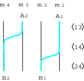
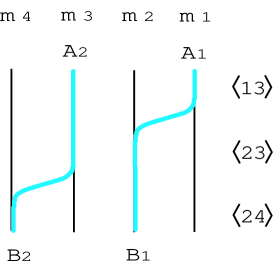
a)	b)

Figure 16: A pair of penetrable walls $\langle 13\leftarrow 24\rangle$ in $N_{\rm C}=2$, $N_{\rm F}=4$ before [a)] and after [b)] exchanging wall positions.

In this brane picture, the existence of penetrable walls becomes very manifest although this phenomenon is complicated in the field theory. The first and the second rows in the matrix (4.41) correspond to the kinky D$p$-brane connecting the first and the second D($p+4$)-branes and the one connecting the third and the fourth ones, respectively. When the positions of two walls are exchanged, the configuration in Fig. 16-a) becomes that in Fig. 16-b), and vice versa. Both configurations in Fig. 16-a) and b) are labeled by $\langle 13\leftarrow 24\rangle$, but different vacua $\langle 13\rangle$ and $\langle 23\rangle$ appear in the intermediate $x^{1}$ in Fig. 16-a) and b), respectively. This is why it is complicated in field theory; By exchanging positions of two walls, the wall at bigger (smaller) $y$ connecting $\langle 13\rangle$ and $\langle 14\rangle$ ($\langle 14\rangle$ and $\langle 24\rangle$) in Fig. 16-a) is transformed to the one at smaller (bigger) $y$ connecting $\langle 23\rangle$ and $\langle 24\rangle$ ($\langle 13\rangle$ and $\langle 23\rangle$) in Fig. 16-b). Therefore walls before and after exchange are not identical in ordinary definition of walls in field theory, since they connect different vacua. However from the brane picture we find that the identities of walls are maintained by this exchange.

There exist two more configurations admitting penetrable walls in the topological sector ${\cal M}^{\langle 12\rangle\leftarrow\langle 34\rangle}$ in this model with $N_{\rm C}=2$ and $N_{\rm F}=4$. They are generated by the moduli matrices

$$H_{0}=\left(\begin{array}[]{cccc}1&0&e^{r}&0\\ 0&1&0&e^{s}\end{array}\right),\hskip 56.9055ptH_{0}=\left(\begin{array}[]{cccc}1&0&0&e^{u}\\ 0&1&e^{v}&0\end{array}\right)$$ (4.50)

with $e^{r},e^{s},e^{u},e^{v}\in{\bf C}^{*}$. The brane configurations corresponding to these matrices are illustrated in Figs. 17 and 18, respectively.

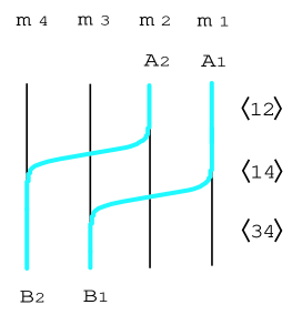
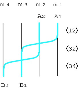
a)	b)

Figure 17: Another pair of penetrable walls in $N_{\rm C}=2$, $N_{\rm F}=4$ $\langle 12\leftarrow 34\rangle$ before [a)] and after [b)] exchanging wall positions.

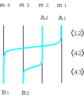
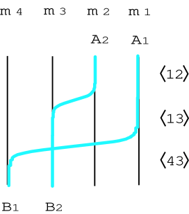
a)	b)

Figure 18: The third pair of penetrable walls $\langle 12\leftarrow 43\rangle$ in $N_{\rm C}=2$, $N_{\rm F}=4$ before [a)] and after [b)] exchanging wall positions.

In Fig. 17 two level-1 compressed walls [the first and the second rows in the first matrix in (4.50)] are penetrable. Note that they are penetrable only when both of them are compressed. In Fig. 18 an elementary wall [the second row in the second matrix in (4.50)] and a level-2 compressed single wall [the first row in the same matrix] are penetrable. For both cases there appear different vacua before and after exchanging positions of two walls.

4.5 Moduli Space and Indices for Non-Abelian Walls

In this subsection we calculate dimensions of the moduli space and its topological sectors in our brane picture. To this end we should classify compressed walls into two classes. The first type is a compressed wall made of single D$p$-brane as in Fig. 14-b). This reduces the number of moduli parameters in the topological sector so we should not consider it to count dimensions. We call this type a “self-compressed brane”. The second type is a compressed wall configuration made of two D$p$-branes as in Fig. 15-b). This occurs if and only if some of $B_{r}$ are not ordered as $B_{1}\leq B_{2}\leq\cdots\leq B_{N_{\rm C}}$ [14]. We call this type a “crossing brane”. The latter can be distinguished from the former by the presence of the reconnection.

The dimension of any topological sector can be counted if there are no compressed walls namely if there are no self-compressed branes and no crossing branes. We call such a configuration a “maximally kinky configuration” in that sector (see Fig. 19). The dimension of a given topological sector can be counted by considering the maximally kinky configuration in that sector, and it is given by two times the number of kinks where the factor two exists because each kink carries the translational and $U(1)$ zero modes. See Fig. 19 as an example.

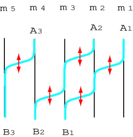
Figure 19: Maximally kinky configuration/Counting the dimension of the moduli space of walls by the brane configuration. The dimension of this example of the topological sector ${\cal M}^{\langle 1,2,4\rangle\leftarrow\langle 3,4,5\rangle}$ can be counted to be $2\times 5=10$ where the factor two comes from the translational and $U(1)$ zero modes.

The maximal topological sector is the topological sector with the maximal dimension. It connects the right-most vacuum $\langle 1,2,\cdots,N_{\rm C}\rangle$ and the left-most vacuum $\langle N_{\rm F}-N_{\rm C},N_{\rm F}-N_{\rm C}+1,\cdots,N_{\rm F}-1,N_{\rm F}\rangle$. The brane configuration for the maximally kinky configuration in the maximal topological sector is illustrated in Fig. 20.

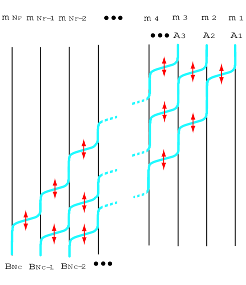
Figure 20: Counting the dimension of the maximal topological sector of the moduli space. It can be counted by the configuration interpolating between the right-most vacuum $\langle A_{1},\cdots,A_{N_{\rm C}}\rangle=\langle 1,2,\cdots,N_{\rm C}\rangle$ and the left-most vacuum $\langle B_{1},\cdots,B_{N_{\rm C}}\rangle=\langle N_{\rm F}-N_{\rm C}+1,\cdots,N_{\rm F}\rangle$.

Then the dimension of the maximal topological sector, or the dimension of the total moduli space, can be calculated from Fig. 20, to yield

$$\dim{\cal M}_{\rm wall} = 2\left[2\sum_{k=1}^{N_{\rm C}}k+N_{\rm C}(N_{\rm F}-1-2N_{\rm C})\right]$$ (4.51)

$$= 2N_{\rm C}(N_{\rm F}-N_{\rm C})=\dim G_{N_{\rm F},N_{\rm C}}.$$

Therefore we recover the field theoretical result (2.16) obtained in [14]. Comparing Fig. 20 for the wall moduli and Fig. 4 for the massless Higgs branch, we can understand that the dimension of the former is the half of the latter.

We now introduce more elegant method to count dimensions of the topological sectors. The index of a given vacuum $\langle A_{1},\cdots,A_{N_{\rm C}}\rangle$ is defined by the real dimension of the maximally kinky configuration in the topological sector which connects that vacuum and the left-most vacuum $\langle N_{\rm F}-N_{\rm C}+1,N_{\rm F}-N_{\rm C}+2,\cdots,N_{\rm F}\rangle$. The moduli matrix for such a configuration is given by

$$\hskip 52.00005ptA_{1}\hskip 31.0001ptA_{r}\hskip 27.0pt$$

$$H_{0} = \sqrt{c}\left(\begin{array}[]{ccccccccccc}\cdots 0&1&*\cdots&*&\cdots&&\cdots e^{v_{1}}\;\;\;\;\;0&\cdots&\hskip 8.53581pt\cdots\hskip 8.53581pt0\\ &&\vdots&&&&\vdots\hskip 28.45274pt\ddots&\;\;\ddots&\\ &&\cdots 0&1&*\cdots&&\cdots&e^{v_{r}}&\underbrace{0\;\cdots\;0}_{N_{\rm C}-r}\\ &&\vdots&&&&\vdots&\hskip 28.45274pt\ddots&&\\ &&&&\cdots 0&1&*\cdots&\cdots&e^{v_{N_{\rm C}}}\\ \end{array}\right){}^{<r}\;,$$

$$\hskip 138.00023ptA_{N_{\rm C}}\hskip 52.00005pt$$

and corresponding brane configuration is illustrated in Fig. 21.

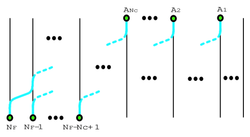
Figure 21: The definition of the indices of vacua. The index for the vacuum $\langle A_{1},\cdots,A_{N_{\rm C}}\rangle$ is defined by the dimension of the configuration interpolating that vacuum and the left-most vacuum $\langle N_{\rm F}-N_{\rm C}+1,\cdots,N_{\rm F}\rangle$.

Then the index can be calculated by either the matrix (4.5) or Fig. 21, to give

$$\nu_{\langle A_{1},\cdots,A_{N_{\rm C}}\rangle}=2\sum_{r=1}^{N_{\rm C}}(N_{\rm F}-N_{\rm C}+r-A_{r})=2N_{\rm C}(N_{\rm F}-N_{\rm C})+N_{\rm C}(N_{\rm C}+1)-2\sum_{r=1}^{N_{\rm C}}A_{r}\;.$$ (4.58)

Actually, this index can be shown to coincide with the Morse index of the wall moduli space, or the base manifold $G_{N_{\rm F},N_{\rm C}}$ of the massless Higgs branch $T^{*}G_{N_{\rm F},N_{\rm C}}$ [50]. Using this index we can calculate the dimension of arbitrary topological sector ${\cal M}^{\langle A_{1},\cdots,A_{N_{\rm C}}\rangle\leftarrow\langle B_{1},\cdots,B_{N_{\rm C}}\rangle}$. If we join a sector connecting $\langle B_{1},\cdots,B_{N_{\rm C}}\rangle$ and the left-most vacuum, ${\cal M}^{\langle B_{1},\cdots,B_{N_{\rm C}}\rangle\leftarrow\langle N_{\rm F}-N_{\rm C}+1,\cdots,N_{\rm F}\rangle}$, to the end of that sector (see Fig. 22), we get the index $\nu_{\langle A_{1},\cdots,A_{N_{\rm C}}\rangle}$.

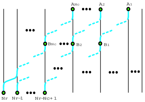
Figure 22: Counting the dimension of a given topological sector of the moduli space of walls using the indices. It can be calculated as the difference of the indices of two vacua by adding the configuration interpolating between the vacuum $\langle B_{1},\cdots,B_{N_{\rm C}}\rangle$ and the the left-most vacuum $\langle N_{\rm F}-N_{\rm C}+1,\cdots,N_{\rm F}\rangle$ into the bottom of that sector.

Therefore the real dimension corresponding to translation and $U(1)$ zero modes is given by the difference between the indices for these vacua:

$$\dim{\cal M}^{\langle A_{1},\cdots,A_{N_{\rm C}}\rangle\leftarrow\langle B_{1},\cdots,B_{N_{\rm C}}\rangle}=\nu_{\langle A_{1},\cdots,A_{N_{\rm C}}\rangle}-\nu_{\langle B_{1},\cdots,B_{N_{\rm C}}\rangle}=2\sum_{r=1}^{N_{\rm C}}(B_{r}-A_{r})\;.$$ (4.59)

This result recovers that of the field theory. For instance the dimension (4.51) of the wall moduli space is given by $\nu_{\langle 1,\cdots,N_{\rm C}\rangle}$.

As discussed in Sec. 4.3 the number of the moduli parameters reduces from the dimension of the topological sector (the dimension of the generic moduli matrix for that sector) whenever there exist crossing branes. These kinds of configurations are not suitable to count the dimension of that topological sector as stated above. We can recognize them by looking at the standard form (2) of the moduli matrix; They occur when $B_{r}$ are not ordered because we have to eliminate some components to fix the world-volume symmetry (2.14) as stated below (2). In [14] such a standard form of the moduli matrix was shown to parameterize a patch with less dimensions in the same topological sector with the generic moduli matrix given by ordered $B_{r}$. The reduced number of dimension of such a patch is given by the number of inversion: the number of sets of ($i,j$) with $\sigma(i)<\sigma(j)$ and $i>j$, where $\sigma$ is an element of the permutation group in Eq. (2.24). To count this number by using brane configurations we define the intersection number by the number of intersections of D$p$-branes with the sign determined as follows. When the $r$-th D$p$-brane (connecting $A_{r}$ at $y\to\infty$ and $B_{r}$ at $y\to-\infty$) intersects anti-clockwise with the $s$-th D$p$-brane, we give $+1$ ($-1$) as an intersection number at that intersection point if $r<s$ ($r>s$). In either case the $r$-th D$p$-brane must be compressed by the s-rule. Then the total intersection number $I$ of a given configuration is defined as the sum of the intersection numbers of all intersection points in that configuration, $I=\sum_{p}{\rm sign}(s-r)$ with $p$ intersection points. By its definition $I$ is non-negative and $I=0$ corresponds to the generic moduli matrix, generating the maximally kinky configuration in general. The important thing is that $I$ is invariant under the change of the positions of kinks provided that reconnections do not occur. For instance the configuration in Fig. 17-b) intersect twice with different sign and therefore it can be changed to Fig. 17-a) without reconnection and is generated by the generic moduli matrix. On the other hand if a reconnection occurs the ordering of $B_{r}$ changes. We find that the number of reduced moduli (the number of inversion) coincides with the total intersection number $I$ of the configuration. For instance both figures in Fig. 16 (Fig. 17) have the intersection number zero, and therefore they are described by the generic moduli matrix with ordered $B_{r}$ (with some zero elements) in ${\cal M}^{\langle 13\rangle\leftarrow\langle 24\rangle}$ (${\cal M}^{\langle 12\rangle\leftarrow\langle 34\rangle}$). On the other hand both the configurations in Fig. 18 have the intersection number one and therefore they are not described by the generic moduli matrix in that sector.

Moduli matrices in the standard form with various ordering of $B_{r}$ contain moduli parameterizing coordinate patches in the topological sector ${\cal M}^{\langle A_{1},\cdots,A_{N_{\rm C}}\rangle\leftarrow\langle B_{1},\cdots,B_{N_{\rm C}}\rangle}$ as in Eq. (2.24). The generic moduli matrix generating the maximally kinky configuration corresponds to the patch $U^{\langle A_{1},\cdots,A_{N_{\rm C}}\leftarrow B_{1},\cdots,B_{N_{\rm C}}\rangle}$ with ordered $B_{r}$ and with $I=0$. Other patches with non-ordered $B_{r}$ are obtained by causing some reconnections. Such the minimum number of reconnections is given by the intersection number $I$. However all configurations in a given topological sector ${\cal M}^{\langle A_{1},\cdots,A_{N_{\rm C}}\rangle\leftarrow\langle B_{1},\cdots,B_{N_{\rm C}}\rangle}$ cannot be classified by only the intersection number or the number of the reconnection because there exist configurations with the same intersection number $I$, which cannot be transformed to each other. The real dimension of arbitrary patch in Eq. (2.24) can be calculated, to yield

$$\dim U^{\langle A_{1},\cdots,A_{N_{\rm C}}\leftarrow B_{\sigma(1)},\cdots,B_{\sigma(N_{\rm C})}\rangle} = \dim{\cal M}^{\langle A_{1},\cdots,A_{N_{\rm C}}\rangle\leftarrow\langle B_{1},\cdots,B_{N_{\rm C}}\rangle}-2I(\sigma)$$ (4.60)

$$= 2\sum_{r=1}^{N_{\rm C}}(B_{r}-A_{r})-2I(\sigma).$$

Before closing this section we discuss Nambu-Goldstone (NG) modes in this system. Wall configurations break the translational symmetry as well as the $U(1)^{N_{\rm F}-1}$ flavor symmetries. Correspondingly there appear massless NG modes on the world-volume theory on the walls. The complex number of moduli parameters coincides with the (real) number of walls and is greater than $N_{\rm F}-1$ in general. The real parts of the moduli parameters correspond to wall positions. The $N_{\rm F}-1$ imaginary parts of the moduli parameters are NG bosons for broken $U(1)^{N_{\rm F}-1}$ symmetry. The rest of imaginary parts are zero modes which are not dictated by the spontaneously broken symmetry, and are called quasi-NG (QNG) bosons [51]. Together with ordinary NG bosons they constitute complex scalar fields needed for unbroken four SUSY. The number of QNG bosons was calculated as

$$N_{\rm QNG}=(N_{\rm C}-1)(\tilde{N}_{\rm C}-1)$$ (4.61)

in the maximal topological sector [14]. We can now easily count the number of QNG bosons in arbitrary topological sector in the brane picture because only one kink carries a $U(1)$ NG zero mode (the overall phase) but the others are QNG zero modes in each intermediate space between adjacent D$(p+4)$-branes. For instance the number of the QNG bosons in Fig. 19 is counted as one because there exist two kinks between the second and the third D($p+4$)-branes. In the case of the maximal topological sector the field theoretical result (4.61) is recovered from Fig. 20.

5 Conclusion and Discussion

We have realized BPS non-Abelian multi-walls in SUSY $U(N_{\rm C})$ gauge theory with $N_{\rm F}$ fundamental hypermultiplets by a brane configuration made of $N_{\rm C}$ kinky fractional D$p$-branes interpolating between $N_{\rm F}$ D($p+4$)-branes separated by amounts corresponding to hypermultiplet mass differences. The tension formula (2.8) for non-Abelian walls has been correctly reproduced as the kinky D-brane tension. The duality between wall configurations in the theories with gauge groups $U(N_{\rm C})$ and $U(\tilde{N}_{\rm C})$ found in field theory in the strong gauge coupling limit has been explained by exchange of the two NS$5$-branes and the Hanany-Witten effect extended to the kinky configurations. Compressing two walls made of two D$p$-branes has been explained by the extended s-rule, and the reconnection (recombination) of these two D$p$-branes has been found to occur. We have shown that the dimensions of the moduli space for non-Abelian walls and its topological sectors can be counted by the brane configuration. In particular we have defined the index which is useful to count their dimensions. The total moduli space ${\cal M}_{\rm wall}\simeq G_{N_{\rm F},N_{\rm C}}$ for non-Abelian walls has been understood to have the dimension of the base space of the Higgs branch in the massless limit, ${\cal M}^{M=0}_{\rm vacua}\simeq T^{*}G_{N_{\rm F},N_{\rm C}}$, of the theory, by comparing these two brane configurations (Figs. 4 and 20). Some more correspondences between field theoretical results and the brane configuration have been clarified.

Let us discuss the several issues in the following.

A brane configuration for a monopole in the Higgs phase. Recently a monopole in the Higgs phase (a confined monopole) has been found [18, 16], and it has been shown to be a 1/4 BPS state realized as a kink in the vortex effective theory. The brane configuration for a monopole in the Higgs phase has been given by Hanany and Tong in Fig. 3 in Appendix A of [5]. (The same configuration has been discussed in [20].) It looks very similar with our brane configuration for walls in Fig. 12-d), but is not identical to ours as explained as follows. The configuration is possible for $p\geq 3$. In the case of $p=3$ the $U(N_{\rm C})$ gauge theory with $N_{\rm F}$ hypermultiplets in four dimensions is realized on D$4$-branes obtained by taking T-duality in the $x^{8}$- and $x^{9}$-directions in Fig. 5. $k$ vortices in that theory are realized as $k$ D$2$-branes stretched between D$4$-branes [4], and the total configuration becomes

$$k 2 0\hskip 11.38109pt3\hskip 22.76219pt8$$ D:

$$N_{\rm C} 4 012\hskip 28.45274pt89$$ D:

$$N_{\rm F} 6 01\hskip 5.69054pt345\hskip 11.38109pt89$$ D:

2 NS$$5 01\hskip 22.76219pt6789\;.$$: (5.1)

In Fig. 12-d) vortices as D$2$-branes are at the segment PQ or RS. In [5] a monopole in the Higgs phase has been realized as a D($p-1$)-brane whose position at the $x^{6}$-coordinate depends on $y=x^{1}$ such that it is at RS when $y\to-\infty$ and at PQ when $y\to+\infty$. At intermediate $y$ the D($p-1$)-brane along $\Delta x^{3}$ cannot end and therefore it bends and extends to the $x^{2}$-coordinate to attach itself to the two NS$5$-branes. Then the configuration becomes very similar with Fig. 12-d). However they are different because branes ending on the NS$5$-branes are the D($p-1$)-branes for their case of kinks inside vortices but the D($p+1$)-branes for our case of kinks themselves. The mass of the monopole can be calculated by the tension of the D($p-1$)-brane. In this case, the contribution from Area (PQSR) is the energy of the vortex and we have to subtract it, contrary to our case for walls. Therefore the monopole mass is calculated from $\Delta x^{2}\Delta x^{6}$ which is the sum of Area (PP^′R^′R) and Area (QQ^′S^′S), to give

$$\tau_{p-1}\Delta x^{2}\Delta x^{6}={\Delta m\over g^{2}}$$ (5.2)

where we have used Eqs. (3.7) and (3.8). This correctly reproduces the mass of a monopole in the Higgs phase [18, 16]. This also coincides with the mass of an ordinary monopole in the Coulomb phase because we get the brane configuration [22] (see also [5, 20]) for a monopole in the Coulomb phase in the limit $\Delta x^{3}\sim c\to 0$.

In Ref. [16] we have given the exact solutions for 1/4 BPS states including all of walls, monopoles and vortices. A brane configuration for these mixed states should be realized as a mixture of ours and the one in [5].

Non-BPS walls. Brane-anti-brane systems are usually unstable. Kink-anti-kink configurations made of a single D$p$-brane are also unstable and decay to a vacuum state. However we can construct stable non-BPS wall configurations by multiple kinky D$p$-branes at least one of which is anti-BPS. This is possible if the flavor $N_{\rm F}$ is greater than four and the color $N_{\rm C}$ and $\tilde{N}_{\rm C}$ are greater than two. The simplest solution can be obtained from the BPS double wall solution (4.44) in the model with $N_{\rm F}=4$ and $N_{\rm C}=2$, by flipping the sign of $y$ in one BPS wall solution, say the (1,1)-element of $\Sigma$ in Eq. (4.44) and the upper-left block in the hypermultiplets $H$, to make it anti-BPS:

$$\Sigma=\left(\begin{array}[]{cc}{m_{1}e^{-2m_{1}y}+m_{2}e^{-2m_{2}y-2{\rm Re}(r)}\over e^{-2m_{1}y}+e^{-2m_{2}y-2{\rm Re}(r)}}&0\\ 0&{m_{3}e^{2m_{3}y}+m_{4}e^{2m_{4}y+2{\rm Re}(s)}\over e^{2m_{3}y}+e^{2m_{4}y+2{\rm Re}(s)}}\end{array}\right),\hskip 14.22636ptW_{y}=0$$ (5.5)

where we have rewritten $r$ as $-r$. The corresponding brane configuration is illustrated in Fig. 23.

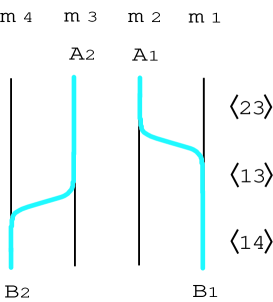
Figure 23: A brane configuration for a non-BPS wall configuration.

We did not examine if the two walls are non-interactive or interactive with each other where interaction may arise from the fluctuation in the off-diagonal elements in $\Sigma$ and/or the off-diagonal blocks in $H$. However we can show that this configuration is likely stable as follows. The solution (5.5) has two complex moduli parameters $r$ and $s$, and positions of the two walls are still given by Eq. (4.45). If the relative position (distance) is large enough, $R\to\infty$, the system reduces to two separated (anti-)BPS walls and gives the stable minimum with respect to the small fluctuations, because the BPS energy bound is saturated at one region and the anti-BPS energy bound at another region, separately. Therefore we find that there does not exist repulsive force between walls for the whole region of $R$. This situation is completely different from the one in [52] where there exists repulsive force between BPS and anti-BPS walls. Then we have two possibilities. If that stable situation continues to hold even for small $R$ the above solution is an absolute minimum, and they are penetrable. If we have a negative potential for small fluctuation at small $R$, it is likely that we have stable bound states. We thus conclude that the non-BPS configuration is most likely to be stable. A concrete discussion is desired.

More subtle configuration which is stable for small fluctuations and metastable for large fluctuations has been considered in the strong gauge coupling limit of the model with $N_{\rm F}=2$ and $N_{\rm C}=1$ [53]. Effective action for these non-BPS walls was constructed by the nonlinear realizations and the Green-Schwarz method [54]. Discussing implications of these states by means of brane configurations in string theory is very interesting and remains as a future problem.

Degenerate masses. Only $U(1)$ Nambu-Goldstone (NG) bosons are localized on walls in our model with non-degenerate masses for hypermultiplets, because $SU(N_{\rm F})$ flavor group is explicitly broken down to $U(1)^{N_{\rm F}-1}$ by non-degenerate masses. If all masses for hypermultiplets are degenerate, the moduli space of vacua becomes the continuously connected manifold ${\cal M}^{M=0}_{\rm vacua}\simeq T^{*}G_{N_{\rm F},N_{\rm C}}$ parametrized by (quasi-) NG bosons for spontaneously broken $SU(N_{\rm F})$. However walls cannot exist in this case. If there are non-degenerate masses even partially, the vacuum manifold consists of disconnected manifolds, and walls can exist. In the case of partially degenerate masses, global symmetry contains non-Abelian groups, instead of $U(1)^{N_{\rm F}-1}$. If vacuum corresponding a degenerate mass appears at a boundary ($y\to\pm\infty$), we need to specify the boundary condition with respect to such a non-Abelian global symmetry, since different points in the space of the global symmetry group are physically distinct points. In such a situation, the NG modes for the broken non-Abelian global symmetry is not a physical normalizable modes localized on walls (but are the bulk modes), since their wave functions extend to the infinity. If vacua with degenerate mass appear at both infinities ($y\to\pm\infty$), the relative rotation modes of two global symmetry transformations are localized on the wall and are physical NG bosons. In this way, one can obtain non-Abelian NG bosons localized on the wall. A field theoretical analysis for the example of $N_{\rm C}=2$ and $N_{\rm F}=4$ with the mass matrix $M={\rm diag}.\,(m,m,-m,-m)$ was discussed by Shifman and Yung [55]. It admits two walls and $U(2)$ NG bosons appear when they are coincident. More detailed analysis for general models with degenerate masses will be reported elsewhere [56].

In the brane picture the vacua are realized by some coincident D($p+4$)-branes. Flavor symmetry is enhanced to non-Abelian by the freedom of open strings on the coincident D($p+4$)-branes. The s-rule allows at most $n$ D$p$-branes to be placed at $n$ coincident D($p+4$)-branes. This drastically changes the dynamics of walls realized as kinky D$p$-branes. For instance, as a result of the s-rule, two walls in the theory [55] with the degenerate masses $M={\rm diag}.\,(m_{1},m_{2},m_{3},m_{4})={\rm diag}.\,(m,m,-m,-m)$ are penetrable (see Fig. 24), although they become impenetrable in generic configuration with mass perturbation $M={\rm diag}.\,(m+\Delta m,m,-m,-m-\Delta m)$ by small mass $\Delta m$.

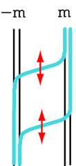
Figure 24: Two walls in the model with $N_{\rm C}=2$ and $N_{\rm F}=4$ and the hypermultiplet masses $M={\rm diag}.\,(m,m,-m,m)$. They are penetrable because the s-rule allows two D$p$-branes can exist inside two coincident D($p+4$)-branes.

Moreover kinky D$p$-branes traveling through the coincident D($p+4$)-branes can break the non-Abelian flavor symmetry arisen from coincidence of D($p+4$)-branes. Thus corresponding non-Abelian NG bosons can be localized on walls. We expect that almost all discussions in this paper such as counting dimensions hold for these cases with degenerate hypermultiplet masses.

Complex, triplet and quartet masses. In this paper we have assumed real masses for hypermultiplets. Actually D$p$-branes with $p=4,3,2,1$ allow real, complex, triplet and quartet masses, respectively. Considering these general masses does not change our discussion drastically because 1/2 BPS states can become kinky along only one spatial coordinate. However these more general mass parameters become important if we consider BPS states preserving less than 1/2 SUSY. For instance a domain wall junction was constructed in [42] as a 1/4 BPS state in the $D=4$, ${\cal N}=2$ SUSY QED with three hypermultiplets with complex masses, embedding the known exact solutions [57]. The theory is realized on a D$3$-brane in the brane configuration

$$1 3 0123$$ D:

$$3 7 01234567$$ D:

$${\bf C}^{2}/{\bf Z}_{2} \hskip 23.33124pt4567\;.$$ ALE: (5.6)

Positions of the three D$7$-branes in the $(x^{8},x^{9})$-plane correspond to three complex masses for hypermultiplets. A junction depends on two coordinates, say $x^{2}$ and $x^{3}$ of the D$3$-brane world volume $x^{0},x^{1},x^{2},x^{3}$. The D$3$-brane position in $x^{8}$ and $x^{9}$ depends on $x^{2}$ and $x^{3}$. The value of the complex adjoint scalar $\Sigma$ of the vector multiplet corresponds to the D$3$-brane position in the ($x^{2}$,$x^{3}$)-plane. At three directions in $x^{2},x^{3}\to\infty$ with keeping $x^{2}/x^{3}$ fixed, there appear three D$7$-branes corresponding to the three possible vacua. Between each three pairs of D$7$-branes, we obtain three different walls represented by kinky D$3$-branes. A junction interpolates among three vacua (D$7$-branes) as a function of the entire $(x^{2},x^{3})$-plane. Therefore the junction is represented by a curved D$3$-brane, interpolating among three D$7$-branes. The world volume is ${\bf R}^{1,1}\times\Sigma$ with a two dimensional surface $\Sigma$. The triplet or quartet masses may be required to construct 1/8 BPS states.

Other representations/gauge groups. Generalization to theories with other representations is an interesting problem. An adjoint hypermultiplet can be introduced if we do not divide the D$(p+4)$-brane world-volume by ${\bf Z}_{2}$. The adjoint hypermultiplet represents positions of the D$p$-branes inside the D$(p+4)$-branes, and the vacua realize the ADHM moduli space for instantons.

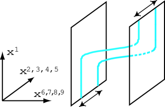
Figure 25: Kinky D-branes for theory with an adjoint hypermultiplet. Walls can move to the $x^{2,3,4,5}$-directions parametrized by adjoint hypermultiplets. Therefore they are mostly penetrable.

It gives (likely) non-normalizable moduli parameters in wall solutions which may be fixed by the boundary conditions and may not be localized on walls (see Fig. 25). Since the positions of the D$p$-branes inside the D$(p+4)$-branes do not coincide in general, non-Abelian walls made of different kinky D$p$-branes are mostly penetrable with each other although all walls made of one kinky D$p$-brane are still impenetrable. If we consider masses for the adjoint hypermultiplet also, the vacuum structure is drastically changed. This is realized by the Scherk-Schwarz dimensional reduction along a common direction of D$p$- and D($p+4$)-brane world-volume using the rotational symmetry of four co-dimensions of the D$p$-branes in the D($p+4$)-branes. The massive adjoint hypermultiplet may participate in constituting walls.

On the other hand if we divide the D$(p+4)$-brane world-volume by ${\bf Z}_{n+1}$ ($A_{n}$-type) or other discrete subgroups of $SU(2)$ ($D_{n}$- or $E$-type), we obtain the quiver gauge theories of $A$ ($D$ or $E$)-types with a product gauge group $U(N_{1})\times U(N_{2})\times\cdots$ and bifundamental hypermultiplets. The behaviors of the fundamental hypermultiplets can be considered to be similar with our model, but those of the bifundamental hypermultiplets are not clear. These may allow richer structures for non-Abelian walls.

Other gauge groups such as $SO(N)$ or $Sp(N)$ can be discussed by introducing orientifold planes. However one immediate question is how to introduce naturally a $U(1)$ factor in the gauge group and a FI term which are needed to obtain discrete vacua.

Breaking to ${\cal N}=1$ SUSY. Here let us consider $D=4$, ${\cal N}=2$ SUSY gauge theory for $p=3$ in the T-dualized brane configuration. We have the corresponding brane configurations, if we replace D$2$-branes by D$4$-branes occupying 01267 and D$4$-branes by D$6$-branes occupying 0134567 in Fig 3. First pull out all the D6-branes to the spatial infinity at $x^{2}=+\infty$. Then there appear $N_{\rm F}-N_{\rm C}$ semi-infinite D$4$-branes attached on the right of the right NS$5$-brane by the Hanany-Witten effect [22]. By rotating one of NS$5$-branes holomorphically in the $v$-$w$ plane, where $v=x^{8}+ix^{9}$ and $w=x^{3}+ix^{4}$, the ${\cal N}=2$ SUSY gauge theory reduces to ${\cal N}=1$ SUSY gauge theory [59, 60]. In the field theory side this deformation corresponds to adding a large mass for the adjoint scalar field $\Sigma$. Relation with the known results for walls [9, 10] in ${\cal N}=1$ SUSY gauge theory would be an interesting subject. In particular the Seiberg duality is realized by exchanging rotated NS$5$-branes. Investigating implications of duality on walls is interesting.

Direct derivation of the wall effective action. It is desirable to replace kinky D-branes by other orthogonal straight D-branes connecting D($p+4$)-branes. This is because it immediately leads to the effective field theory on non-Abelian walls in the D-brane picture; If we could do this it would be possible to construct the moduli space for non-Abelian walls by the vacuum conditions on the effective theory as other solitons like instantons [28], monopoles [29] and vortices [4]. It might be possible to understand not only their dimensionality but also why the wall moduli space ${\cal M}_{\rm wall}\simeq G_{N_{\rm F},N_{\rm C}}$ is a special Lagrangian submanifold of the Higgs branch ${\cal M}_{\rm vacua}^{M=0}\simeq T^{*}G_{N_{\rm F},N_{\rm C}}$ in the massless limit. Also this may be related to the problem of gauge field localization, because the world-volume theory on D-branes contains localized gauge fields by its definition.

Higher derivative corrections. Let us discuss two points on higher derivative corrections. The first point is the higher derivative corrections coming from the Dirac-Born-Infeld (DBI) action on D$p$-branes. In the case of monopoles, BPS solutions in the field theory are not modified (up to some order) when the theory is promoted to the DBI action which includes higher derivative terms. Therefore they can be understood as solitons in the DBI theory called the BIons [61]. It is very interesting to investigate if wall solutions are also unchanged when we promote the theory to the DBI action and if we can interpret them as BIons with co-dimension one.

The second point is higher derivative corrections in the effective action on walls. The Manton’s effective theory on the non-Abelian walls was constructed as (5.7) in [13, 14] in the strong gauge coupling limit:

$${\cal L}_{\rm walls}^{g\to\infty}=c\int d^{4}\theta\int dy\ \log\det\Omega_{g\to\infty}=c\int d^{4}\theta\int dy\ \log\det(H_{0}e^{2My}H_{0}{}^{\dagger})\;$$ (5.7)

where we have promoted the moduli matrix to $D=4$, ${\cal N}=1$ chiral superfield $H_{0}(x,\theta,\bar{\theta})$ satisfying $\bar{D}_{\dot{\alpha}}H_{0}=0$, and $d^{4}\theta$ denotes integration over superspace. It is valid at low energies up to two derivative terms because it is constructed under the assumption of slowly moving collective coordinates. The higher derivative corrections to this action is expected to exist but they are not known in general. If we could realize walls by straight D-branes as stated above but not by kinky D-branes, higher derivative corrections to this action would be realized by the DBI action.

Embedding to SUGRA. Wall solutions for $U(1)$ gauge theory in the strong gauge coupling limit were embedded into $D=5$ SUGRA [62]. There it was shown that matter parts of solutions are not changed. These works may be extended to full kinky D-brane configuration in non-Abelian gauge theory and/or at finite gauge coupling constant, coupled with SUGRA. It would be interesting to investigate the AdS/CFT correspondence in these configurations.

References

- [1] M. F. Atiyah, N. J. Hitchin, V. G. Drinfeld and Yu. I. Manin, Phys. Lett. A 65, 185 (1978).
- [2] W. Nahm, Phys. Lett. B 90, 413 (1980).
- [3] N. Seiberg and E. Witten, Nucl. Phys. B 426, 19 (1994) [Erratum-ibid. B 430, 485 (1994)] [arXiv:hep-th/9407087]; Nucl. Phys. B 431, 484 (1994) [arXiv:hep-th/9408099]; N. Seiberg, Nucl. Phys. B 435, 129 (1995) [arXiv:hep-th/9411149].
- [4] A. Hanany and D. Tong, JHEP 0307, 037 (2003) [arXiv:hep-th/0306150].
- [5] A. Hanany and D. Tong, JHEP 0404, 066 (2004) [arXiv:hep-th/0403158].
- [6] M. Eto, M. Nitta and N. Sakai, Nucl. Phys. B 701, 247 (2004) [arXiv:hep-th/0405161].
- [7] R. Auzzi, S. Bolognesi, J. Evslin, K. Konishi and A. Yung, Nucl. Phys. B 673, 187 (2003) [arXiv:hep-th/0307287].
- [8] M. A. Shifman, Phys. Rev. D 57, 1258 (1998) [arXiv:hep-th/9708060]; M. A. Shifman and M. B. Voloshin, Phys. Rev. D 57, 2590 (1998) [arXiv:hep-th/9709137].
- [9] B. S. Acharya and C. Vafa, arXiv:hep-th/0103011.
- [10] A. Ritz, M. Shifman and A. Vainshtein, Phys. Rev. D 66, 065015 (2002) [arXiv:hep-th/0205083]; Phys. Rev. D 70, 095003 (2004) [arXiv:hep-th/0405175]; A. Ritz, JHEP 0310, 021 (2003) [arXiv:hep-th/0308144].
- [11] J. P. Gauntlett, D. Tong and P. K. Townsend, Phys. Rev. D 64, 025010 (2001) [arXiv:hep-th/0012178].
- [12] D. Tong, Phys. Rev. D 66, 025013 (2002) [arXiv:hep-th/0202012]; JHEP 0304, 031 (2003) [arXiv:hep-th/0303151]; K. S. M. Lee, Phys. Rev. D 67, 045009 (2003) [arXiv:hep-th/0211058].
- [13] Y. Isozumi, M. Nitta, K. Ohashi and N. Sakai, Phys. Rev. Lett. 93, 161601 (2004) [arXiv:hep-th/0404198].
- [14] Y. Isozumi, M. Nitta, K. Ohashi and N. Sakai, Phys. Rev. D 70, 125014 (2004) [arXiv:hep-th/0405194].
- [15] Y. Isozumi, M. Nitta, K. Ohashi and N. Sakai, in the proceedings of 12th International Conference on Supersymmetry and Unification of Fundamental Interactions (SUSY 04), Tsukuba, Japan, 17-23 Jun 2004, edited by K. Hagiwara et al. (KEK, 2004) p.1 - p.16 [arXiv:hep-th/0409110]; to appear in the proceedings of “NathFest” at PASCOS conference, Northeastern University, Boston, Ma, August 2004 [arXiv:hep-th/0410150].
- [16] Y. Isozumi, M. Nitta, K. Ohashi and N. Sakai, Phys. Rev. D 71, 065018 (2005) [arXiv:hep-th/0405129].
- [17] J. P. Gauntlett, R. Portugues, D. Tong, and P.K. Townsend, Phys. Rev. D 63, 085002 (2001) [arXiv:hep-th/0008221]; M. Shifman and A. Yung, Phys. Rev. D 67, 125007 (2003) [arXiv:hep-th/0212293].
- [18] D. Tong, Phys. Rev. D 69, 065003 (2004) [arXiv:hep-th/0307302]; R. Auzzi, S. Bolognesi, J. Evslin and K. Konishi, Nucl. Phys. B 686, 119 (2004) [arXiv:hep-th/0312233]; M. Shifman and A. Yung, Phys. Rev. D 70, 045004 (2004) [arXiv:hep-th/0403149].
- [19] M. A. C. Kneipp and P. Brockill, Phys. Rev. D 64, 125012 (2001) [arXiv:hep-th/0104171]; M. A. C. Kneipp, Phys. Rev. D 68, 045009 (2003) [arXiv:hep-th/0211049]; Phys. Rev. D 69, 045007 (2004) [arXiv:hep-th/0308086]; arXiv:hep-th/0401234.
- [20] R. Auzzi, S. Bolognesi and J. Evslin, JHEP 0502, 046 (2005) [arXiv:hep-th/0411074].
- [21] M. Eto, Y. Isozumi, M. Nitta, K. Ohashi and N. Sakai, arXiv:hep-th/0412048
- [22] A. Hanany and E. Witten, Nucl. Phys. B 492, 152 (1997) [arXiv:hep-th/9611230].
- [23] E. Witten, Nucl. Phys. B 500, 3 (1997) [arXiv:hep-th/9703166].
- [24] K. Hori, H. Ooguri and Y. Oz, Adv. Theor. Math. Phys. 1, 1 (1998) [arXiv:hep-th/9706082].
- [25] T. Nakatsu, K. Ohta, T. Yokono and Y. Yoshida, Nucl. Phys. B 519, 159 (1998) [arXiv:hep-th/9707258].
- [26] T. Nakatsu, K. Ohta, T. Yokono and Y. Yoshida, Mod. Phys. Lett. A 13, 293 (1998) [arXiv:hep-th/9711117].
- [27] A. Giveon and D. Kutasov, Rev. Mod. Phys. 71, 983 (1999) [arXiv:hep-th/9802067].
- [28] E. Witten, Nucl. Phys. B460, 541 (1996) [arXiv:hep-th/9511030]; M. R. Douglas, arXiv:hep-th/9512077.
- [29] M. B. Green and M. Gutperle, Phys. Lett. B 377, 28 (1996) [arXiv:hep-th/9602077]; D. E. Diaconescu, Nucl. Phys. B 503, 220 (1997) [arXiv:hep-th/9608163].
- [30] N. Nekrasov and A. Schwarz, Commun. Math. Phys. 198, 689 (1998) [arXiv:hep-th/9802068]; K. Furuuchi, Prog. Theor. Phys. 103, 1043 (2000) [arXiv:hep-th/9912047].
- [31] A. Hashimoto and K. Hashimoto, JHEP 9911, 005 (1999) [arXiv:hep-th/9909202]; K. Hashimoto, H. Hata and S. Moriyama, JHEP 9912, 021 (1999) [arXiv:hep-th/9910196]; D. J. Gross and N. A. Nekrasov, JHEP 0007, 034 (2000) [arXiv:hep-th/0005204].
- [32] D. J. Gross and N. A. Nekrasov, JHEP 0103, 044 (2001) [arXiv:hep-th/0010090]; M. Hamanaka, Phys. Rev. D 65, 085022 (2002) [arXiv:hep-th/0109070]; arXiv:hep-th/0303256.
- [33] N. D. Lambert and D. Tong, Nucl. Phys. B 569, 606 (2000) [arXiv:hep-th/9907098].
- [34] T. Eguchi and A. J. Hanson, Phys. Lett. B 74, 249 (1978); T. Eguchi, P. B. Gilkey and A. J. Hanson, Phys. Rept. 66, 213 (1980).
- [35] P. B. Kronheimer and H. Nakajima, Math. Ann. 288, 263 (1990); H. Nakajima, Duke Math. J. 76, 365 (1994).
- [36] M. R. Douglas and G. W. Moore, arXiv:hep-th/9603167; C. V. Johnson and R. C. Myers, Phys. Rev. D 55, 6382 (1997) [arXiv:hep-th/9610140].
- [37] K. Hashimoto and S. Nagaoka, JHEP 0306, 034 (2003) [arXiv:hep-th/0303204]; K. Hashimoto and W. Taylor, JHEP 0310, 040 (2003) [arXiv:hep-th/0307297]; S. Nagaoka, JHEP 0402, 063 (2004) [arXiv:hep-th/0312010].
- [38] N. J. Hitchin, A. Karlhede, U. Lindström and M. Roček, Commun. Math. Phys. 108, 535 (1987).
- [39] U. Lindström and M. Roček, Nucl. Phys. B 222 (1983) 285.
- [40] M. Arai, M. Nitta and N. Sakai, Prog. Theor. Phys. 113, 657 (2005) [arXiv:hep-th/0307274]; to appear in the Proceedings of the 3rd International Symposium on Quantum Theory and Symmetries (QTS3), September 10-14, 2003, [arXiv:hep-th/0401084]; to appear in the Proceedings of the International Conference on “Symmetry Methods in Physics (SYM-PHYS10)” held at Yerevan, Armenia, 13-19 Aug. 2003 [arXiv:hep-th/0401102]; to appear in the Proceedings of SUSY 2003 held at the University of Arizona, Tucson, AZ, June 5-10, 2003 [arXiv:hep-th/0402065].
- [41] G. Carlino, K. Konishi and H. Murayama, JHEP 0002, 004 (2000) [arXiv:hep-th/0001036]; Nucl. Phys. B 590, 37 (2000) [arXiv:hep-th/0005076].
- [42] K. Kakimoto and N. Sakai, Phys. Rev. D 68, 065005 (2003) [arXiv:hep-th/0306077].
- [43] Y. Isozumi, K. Ohashi, and N. Sakai, JHEP 0311, 060 (2003) [arXiv:hep-th/0310189].
- [44] Y. Isozumi, K. Ohashi, and N. Sakai, JHEP 0311, 061 (2003) [arXiv:hep-th/0310130].
- [45] L. Alvarez-Gaume and D. Z. Freedman, Commun. Math. Phys. 91, 87 (1983).
- [46] E. Abraham and P. K. Townsend, Phys. Lett. B 291, 85 (1992).
- [47] M. Arai, M. Naganuma, M. Nitta, and N. Sakai, Nucl. Phys. B 652, 35 (2003) [arXiv:hep-th/0211103]; “BPS Wall in N=2 SUSY Nonlinear Sigma Model with Eguchi-Hanson Manifold” in Garden of Quanta - In honor of Hiroshi Ezawa, Eds. by J. Arafune et al. (World Scientific Publishing Co. Pte. Ltd. Singapore, 2003) pp 299-325, [arXiv:hep-th/0302028]; M. Arai, E. Ivanov and J. Niederle, Nucl. Phys. B 680, 23 (2004) [arXiv:hep-th/0312037].
- [48] J. P. Gauntlett, D. Tong, and P.K. Townsend, Phys. Rev. D 63 085001 (2001) [arXiv:hep-th/0007124].
- [49] M. Naganuma, M. Nitta and N. Sakai, Grav. Cosmol. 8, 129 (2002) [arXiv:hep-th/0108133]; R. Portugues and P. K. Townsend, JHEP 0204, 039 (2002) [arXiv:hep-th/0203181].
- [50] M. Eto, Y. Isozumi, M. Nitta, K. Ohashi, K. Ohta, N. Sakai and Y. Tachikawa, unpublished.
- [51] W. Buchmuller, S. T. Love, R. D. Peccei and T. Yanagida, Phys. Lett. B 115, 233 (1982); W. Buchmuller, R. D. Peccei and T. Yanagida, Phys. Lett. B 124, 67 (1983); Nucl. Phys. B 227, 503 (1983); K. Higashijima, M. Nitta, K. Ohta and N. Ohta, Prog. Theor. Phys. 98, 1165 (1997) [arXiv:hep-th/9706219]; M. Nitta, Int. J. Mod. Phys. A 14, 2397 (1999) [arXiv: hep-th/9805038]; K. Higashijima and M. Nitta, Prog. Theor. Phys. 103, 635 (2000) [arXiv:hep-th/9911139]; K. Furuta, T. Inami, H. Nakajima and M. Nitta, Prog. Theor. Phys. 106, 851 (2001) [arXiv:hep-th/0106183].
- [52] D. Binosi and T. ter Veldhuis, Phys. Rev. D 63, 085016 (2001) [arXiv:hep-th/0011113].
- [53] M. Eto, N. Maru and N. Sakai, Nucl. Phys. B 696, 3 (2004) [arXiv:hep-th/0404114]; in the proceedings of 12th International Conference on Supersymmetry and Unification of Fundamental Interactions (SUSY 04), Tsukuba, Japan, 17-23 Jun 2004, edited by K. Hagiwara et al. (KEK, 2004) p.849 - p.852 [arXiv:hep-th/0409152].
- [54] T. E. Clark, M. Nitta and T. ter Veldhuis, Phys. Rev. D 67, 085026 (2003) [arXiv:hep-th/0208184]; Phys. Rev. D 69, 047701 (2004) [arXiv:hep-th/0209142]; Phys. Rev. D 70, 105005 (2004) [arXiv:hep-th/0401163]; Phys. Rev. D 71, 025017 (2005) [arXiv:hep-th/0409030]; Phys. Rev. D 70, 125011 (2004) [arXiv:hep-th/0409151].
- [55] M. Shifman and A. Yung, Phys. Rev. D 70, 025013 (2004) [arXiv:hep-th/0312257].
- [56] M. Eto, Y. Isozumi, M. Nitta, K. Ohashi and N. Sakai, in preparation.
- [57] H. Oda, K. Ito, M. Naganuma and N. Sakai, Phys. Lett. B 471, 140 (1999) [arXiv:hep-th/9910095]; K. Ito, M. Naganuma, H. Oda and N. Sakai, Nucl. Phys. B 586, 231 (2000) [arXiv:hep-th/0004188]; Nucl. Phys. Proc. Suppl. 101, 304 (2001) [arXiv:hep-th/0012182]; M. Naganuma, M. Nitta and N. Sakai, Phys. Rev. D 65, 045016 (2002) [arXiv:hep-th/0108179]; in the proceedings of 3rd International Sakharov Conference On Physics, 24-29 Jun 2002, Moscow, Russia, edited by A. Semikhatov et al. (Scientific World Pub., 2003) p.537 - p.549 [arXiv:hep-th/0210205].
- [58] M. Naganuma and M. Nitta, Prog. Theor. Phys. 105, 501 (2001) [arXiv:hep-th/0007184].
- [59] S. Elitzur, A. Giveon and D. Kutasov, Phys. Lett. B 400, 269 (1997) [arXiv:hep-th/9702014].
- [60] J. L. F. Barbon, Phys. Lett. B 402, 59 (1997) [arXiv:hep-th/9703051].
- [61] C. G. Callan,Jr. and J. M. Maldacena, Nucl. Phys. B 513, 198 (1998); G. W. Gibbons, Nucl. Phys. B 514, 603 (1998); A. Hashimoto, Phys. Rev. D 57, 6441 (1998).
- [62] M. Arai, S. Fujita, M. Naganuma and N. Sakai, Phys. Lett. B 556, 192 (2003) [arXiv:hep-th/0212175]; to appear in the proceedings of International Seminar on Supersymmetries and Quantum Symmetries SQS 03, Dubna, Russia, 24-29 Jul 2003, [arXiv:hep-th/0311210]; to appear in the proceedings of SUSY 2003: SUSY in the Desert: 11th Annual International Conference on Supersymmetry and the Unification of Fundamental Interactions, Tucson, Arizona, 5-10 Jun 2003. [arXiv:hep-th/0402040]; M. Eto, S. Fujita, M. Naganuma and N. Sakai, Phys. Rev. D 69, 025007 (2004) [arXiv:hep-th/0306198].