The Phase Transition between Caged Black Holes and Black Strings – A Review

Abstract:

Black hole uniqueness is known to fail in higher dimensions, and the multiplicity of black hole phases leads to phase transitions physics in General Relativity. The black-hole black-string transition is a prime realization of such a system and its phase diagram has been the subject of considerable study in the last few years. The most surprising results seem to be the appearance of critical dimensions where the qualitative behavior of the system changes, and a novel kind of topology change. Recently, a full phase diagram was determined numerically, confirming earlier predictions for a merger of the black-hole and black string phases and giving very strong evidence that the end-state of the Gregory-Laflamme instability is a black hole (in the dimension range $5\leq D\leq 13$). Here this progress is reviewed, illustrated with figures, put into a wider context, and the still open questions are listed.

1 Introduction

In this introduction we will present the general background for studying General Relativity in higher dimensions and the novel field of phase transitions in General Relativity. We will list the systems known to exhibit phase transitions, and take the opportunity to discuss the rotating black ring before we proceed to concentrate on our system of choice, the black-hole black-string transition.

Why study GR in higher dimensions? There are several good reasons to study General Relativity (GR) in higher dimensions, namely $D>4$, where $D$ is the total space-time dimension. From a theoretical point of view there is nothing in GR that restricts us to $D=4$. On the contrary, the theory is independent of $D$, and $D$ should be considered as a parameter. It is common practice in theoretical physics to explore large regions of parameter space of a theory in order to enhance its understanding, rather than restrict to the experimental values and GR should be no exception. For example, in the study of gauge theories it is standard to consider various possibilities for the gauge group and matter content which differ from the standard model.

Additional reasons to study higher dimensional GR include string theory and the phenomenological scenario of “large extra dimensions”, as we proceed to discuss. String theory has a “built-in” preference for higher dimensional spacetimes with 10 (the ”critical dimension”) or 11 dimensions, where the extra dimensions must be compactified. This preference originates in the cancellation of the conformal (quantum) anomaly in 10d which is necessary for the consistency of weakly coupled string theories. The “large extra dimensions” scenario (which is presumably string theory inspired) stresses the following important realizations: that to date gravity is measured only down to $1\mu$–1mm range (which is an “astronomically” poor resolution relative to the one we have for other forces), that it is quite consistent to assume the existence of a compact dimension(s) smaller than the experimental bound and that the situation can be rectified only by improving gravitational and accelerator experiments.

The novel feature - non-uniqueness of black objects. Often when we generalize a problem to allow for an arbitrary dimension the qualitative features do not change and thus the generalization does not produce “new physics”, even if the quantitative expressions are different. However, in GR we do find qualitative changes. If we roughly divide the field of General Relativity into black holes, gravitational waves and cosmology, we find a qualitative change in the first of these categories: one of the basic properties of 4d black holes changes, namely black hole uniqueness.

Here we should digress to make the distinction between two closely related black hole notions: “no hair” and “uniqueness” (see for example [2]). “No hair” denotes the feature that the space of black hole solutions has a small dimension usually parameterized by asympototically measured quantities (mass, angular momentum and electric charge, for example) much like macroscopic thermodynamical variables. In this respect a black hole strongly contrasts with a non-black-hole star which typically has a much larger number of characteristics such as its internal matter ingredients each with its own equation of state and spatial distribution possibly resulting in an unbounded number of independent multipoles for mass, charge and angular momentum. Whether this “no-hair” property continues to hold for higher dimensional black holes could depend on the way one chooses to generalize it. If one generalizes “no hair” to mean that the solutions are determined in term of a small number of (not necessarily conserved) asymptotic data then it continues to hold in higher dimensions as far as we know. However, if one would choose the more restrictive definition which requires conserved charges then this property fails in higher dimensions as was demonstrated in the generalized rotating black ring [3, 4, 5], whose parameters include some non-conserved dipole charges.

“Uniqueness” on the other hand is the more specialized statement that a choice of all of these asymptotic black hole parameters selects a unique black hole rather than a discrete set. In other words, that only a single branch of solutions exists. In 4d uniqueness was proven to hold, namely that given the mass, charge and angular momentum (satisfying some inequalities to ensure the existence of a solution with no naked singularities) there is a unique black hole. However, the proof relies heavily on properties which are special to 4d: Hawking’s proof that the horizon topology has to be ${\bf S}^{2}$ and the simplifying gauge choices of Weyl-Papapetrou and Ernst (see [6] for references to original papers and reviews and for a speculative generalization of uniqueness to higher dimensions). See [7, 8] for a determination of the allowed horizon topologies in certain $D>4$.

The breakdown of black hole uniqueness in higher dimensions implies the coexistence of several phases with the same asymptotic charges on a non-trivial phase diagram. Phase transitions between the various phases should occur as parameters are changed. As always one may define the order of the phase transition. It could be a first order transition in which case it is triggered non-perturbatively by a competition of entropies between two phases which are separated by a finite distance in configuration space, or it could be of second or higher order, in which case it is triggered by perturbative tachyons and the transition is smooth (see subsection 3.2).

Such first order transitions would be accompanied by an exceptional release of energy, sometimes called a thunderbolt, simply since the total mass of the final state must be lower than or equal to that of the initial state and the excess energy must be lost through radiation. Moreover, exact mass equality is highly unlikely, but rather a loss of mass is natural as spacetime would undergo violent changes including sometimes the roll-down of a tachyonic mode.

The two systems. To date we know of two systems with higher dimensional non-uniqueness resulting in non-trivial phase transition physics

• The rotating ring

• The black-hole black-string transition

The latter was chosen for a thorough study of its phase structure which is the subject of this review, presumably since it is somewhat simpler to analyze on account of the smaller number of metric functions and its higher degree of symmetry. Before proceeding to analyze it in detail, we discuss the other example, the black ring.

The rotating black ring lives in the flat (and topologically trivial) 5d background. Spherical rotating black holes solutions in higher dimensions, which generalize the 4d Kerr solution were already found in 1986 by Myers and Perry [10]. These solutions have an ${\bf S}^{3}$ horizon topology in 5d and display a maximal angular momentum (at fixed mass). In 2001 Emparan and Reall [11] discovered a beautiful solution, the ring, with horizon topology ${\bf S}^{2}\times{\bf S}^{1}$, and with an angular momentum which is bounded from below, but not from above (at fixed mass). Figure 1 shows the regions on the angular momentum axis which are occupied by the various phases, and one notes that there is a middle region where three phases coexist – one black hole and two rings. Unlike the black string, rotating ring solutions are known only in 5d, presumably due to the special property that in 5d the centrifugal potential and the (Newtonian) gravitation potential have the same ($1/r^{2}$) $r$-dependence.

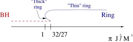
Figure 1: In asymptotically flat 5d spacetime uniqueness is violated by the co-existence of the rotating black hole and the rotating black ring. The figure shows the range of existence of each phase on the dimensionless angular momentum axis. Note that for $1\leq\pi\,J^{2}/M^{3}\leq 32/27$ three phases co-exist.

For some time it was not clear whether the black ring is stable, and despite some recent findings the issue is not settled yet. In 2004 charged rings were shown to be BPS [12] and hence plausibly “super-stable” (that is, non-perturbatively stable). Although the stability of the original non-BPS ring of [11] is still undetermined (however, see [13] for interesting partial results on stability), there is comfort in knowing that some of its closest relatives which share many of their outstanding properties are plausibly stable. Soon after, several groups made progress in obtaining larger families of ring solutions, both BPS [14, 4, 5, 15] and non-BPS [16], all of them restricted to 5d. Moreover, the inclusion of non-conserved dipole moments in [5] demonstrates the “no-hair” principle in higher dimensions must be generalized at least to allow for non-conserved quantities.

As the recent discovery of families of black rings demonstrates, the black ring may hold further surprises. In particular, we do not know the full parameter space for rings, and we know close to nothing about the associated phase transitions. Thus rotating rings constitute a promising and active field of research.

Outline. At this point we set aside the topic of black rings until the discussion section and we turn in the next section to the other example for non-uniqueness, the black-hole black-string transition which is the main topic of this review. In section 2 the physical set-up is described and the questions of interest are formulated. In section 3 we describe the analytic considerations that culminate in subsection 3.5 to a certain suggestive qualitative form of the phase diagram which is compared there with numerical data. Section 4 describes the quantitative tools that were employed in order to obtain solutions, including both numerical and analytic methods. Finally, related work is described in section 5 and we conclude with a summary of the results and a discussion of open questions in section 6.

2 Set-up and formulation of questions

2.1 Background metric and phases

Background metric. We consider a background with extra compact dimensions. In such a background one expects to find several phases of black objects depending on the relative size of the object and the relevant length scales in the compact dimensions. For simplicity we discuss here pure GR (the only field is the metric) with no cosmological constant. Thus the backgrounds considered are of the form $\mathbb{R}^{d-1,1}\times X^{p}$ where $X^{p}$ is any $p$-dimensional compact Ricci-flat manifold, $d$ is the number of extended spacetime dimensions, and the total spacetime dimension is $D=d+p$.

The simplest compactifying manifold is a single compact dimension $X={\bf S}^{1}$, and accordingly that was the $X$ considered in most of the research so far. ${\bf S}^{1}$ was chosen not only for its simplicity but also since while more involved $X$ will have several phases of black objects, the phase transition physics between any two specific phases is expected to be essentially similar (generically) to the ${\bf S}^{1}$ case. Some research was devoted to $X={\bf T}^{p}$, the $p$-dimensional torus [17, 18], and we shall discuss it later. Other possibilities for $X$ include K3 and Calabi-Yau threefolds, as well as Ricci-flat spaces $X$ which are not supersymmetric.

Thus we consider a background with a single compact dimension of size $L$, namely $\mathbb{R}^{d-1,1}\times{\bf S}^{1}$, and $D=d+1\geq 5$ (the lower bound on $D$ is set in order to avoid spacetimes with 2 or less extended spatial dimensions where the presence of a massive source is inconsistent with asymptotic flatness, see [19, 20, 21] for a limited analogue in $D=4$).

Black objects. The non-rotating black objects in which we are interested are static and spherically symmetric. Thus, the essential geometry is 2d after suppressing time and the angular coordinates in the extended dimensions. Our coordinates are defined in figure 2.

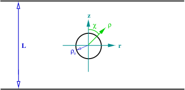
Figure 2: Definition of coordinates. For backgrounds with a single compact dimension the essential geometry is 2d after suppressing time and angular coordinates in the extended dimensions. The cylindrical coordinates $(r,z)$ are defined such that $z\sim z+L$ is the coordinate along the compact dimension and $r$ is the radial coordinate in the extended spatial directions. For black holes we define another set of local coordinates $(\rho,\chi)$, defined only for $\rho\leq L/2$, which are radial coordinates in the 2d plane with origin at the center of the BH.

Such solutions are characterized by 3 dimensionful parameters $M,\,L$ and $G_{N}$ where $M$ is the mass of the black object (measured in the asymptotic $d$ dimensional spacetime, and the detailed expression is given in 18), and $G_{N}$ is Newton’s constant. These define a single dimensionless parameter

$$\mu:={G_{N}\,M\over L^{D-3}}~{}.$$ (1)

Alternatively one may use a different parameterization of the solutions such as replacing $M$ by $\beta$, the inverse temperature. Correspondingly one may define another dimensionless parameter

$$\mu_{\beta}\propto{\beta\over L}~{},$$ (2)

where the proportionality factor may be chosen later by convenience. In thermodynamic terms, the parameter (1) or (2) is the “control parameter” of the system, and the choice between these two depends on whether one prefers the micro-canonical or canonical ensembles, respectively.

In this background one expects at least two phases of black object solutions: when $\mu\ll 1$, namely the size of the black object is small (compared to $L$ the size of the extra dimension) one expects the region near the object to closely resemble a $D$-dimensional black hole, while as one increases the mass one expects that at some point the black hole will no longer fit in the compact dimension and a black string, whose horizon winds around the compact dimension will be formed. The precise distinction between these two phases is give by
Definition: We distinguish between the black hole (BH) and the black string according to their horizon topology which is either spherical — ${\bf S}^{D-2}$ or cylindrical — ${\bf S}^{d-2}\times X$, respectively.
These phases are illustrated in figures 3,4,5(b). We shall sometimes refer to such a black hole localized in a compact dimension as a “caged black hole”.

Applications. Before proceeding to discuss the phases in more detail, let us mention some applications that contribute to its importance, beyond its considerable intrinsic value. In String Theory it has attracted continued interest, particularly regarding the thermodynamic phase diagram for various gravity theories and/or field theories [22, 23] which are related by dualities to the higher dimensional origin of brane solitons (such as the M-theory origin of string branes), where the physics is significantly affected by the question whether they are localized in the compact dimensions or wrap them. Another field of application is black holes on brane-worlds [24, 25], a problem closely related to the one discussed here, only the background in which the black objects live includes not only an extra dimension but also a “phenomenological” brane localized in that dimension and carrying the fields of the standard model.

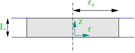
Figure 3: The uniform black string. $r_{0}$ is its Schwarzschild radius.

We now proceed to discuss the two phases with more detail.
The black string. We can readily write down solutions which describe uniform black strings (see figure 3)

$$ds^{2}=ds^{2}_{\mbox{Schw}}+ds^{2}_{X}$$ (3)

where $ds^{2}_{X}$ is the metric on $X$, which for our central example, an ${\bf S}^{1}$ parameterized by the coordinate $z$, is just

$$ds^{2}_{X}=dz^{2}~{},$$ (4)

and $ds^{2}_{\mbox{Schw}}$ is the $d$-dimensional Schwarzschild black hole (also known as Schwarzschild-Tangherlini [26]), which is given by

$$ds^{2}_{\mbox{Schw}}=-f(\rho)\,dt^{2}+\frac{1}{f(\rho)}\,d\rho^{2}+\rho^{2}\,d\Omega_{d-2}^{2}$$ (5)

where

$$f(\rho)=1-\frac{\rho_{0}^{d-3}}{\rho^{d-3}}~{},$$ (6)

$d\Omega_{d-2}^{2}$ is the metric on the sphere $S^{d-2}$

$$d\Omega_{d-2}^{2}=d\chi^{2}+\sin^{2}\chi\,d\theta_{1}^{2}+...+(\sin^{2}\chi\,\sin^{2}\theta_{1}...\sin^{2}\theta_{d-4})\,d\theta_{d-3}^{2}~{}.$$ (7)

$\rho_{0}$ is related to the black hole mass, $M$, via [10]

$$\rho_{0}^{d-3}=\frac{16\,\pi\,G_{d}\,M}{(d-2)\,\Omega_{d-2}}~{},$$ (8)

where $G_{d}$ is the $d$-dimensional Newton constant, and $\Omega_{d-1}=d{\pi^{d/2}\over(d/2)!}=\frac{2\,\pi^{\frac{d}{2}}}{\Gamma(\frac{d}{2})}$ is the area of a unit sphere $S^{d-1}$. The relation between $r_{0}$ and the inverse temperature $\beta$ is

$$\beta={2\,\pi\over\kappa}={4\,\pi\over f^{\prime}(r_{0})}={4\,\pi\,r_{0}\over d-3}~{}.$$ (9)

These metrics are Ricci flat as a result of being a direct product of Ricci flat metrics. They are called “uniform” for being a direct product with $X$ (moreover, for ${\bf S}^{1}$ the full metric is $z$-independent). Later we will encounter also non-uniform strings (see figure 5(b)). Note that for general $p>1$ (namely dim$(X)$) these metrics actually describe $p$-branes rather than strings.

The uniform black string solution is valid for any $r_{0}$ (and fixed $X$). However, we shall soon see that for “thin” enough strings, namely small enough $r_{0}$, an instability develops.

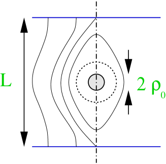
Figure 4: A caged black hole (BH). Newtonian equipotential lines are shown.

Caged black holes. One expects localized black hole (BH) solutions to exist (see figure 4), intuitively obtained by constructing a black hole locally without ever being “aware” of the compactness of the some of the dimensions, at least as long as the black hole is much smaller than the compact dimensions (and the number of extended spacetime dimension is $d\geq 4$ to avoid problems with asymptotics) .

As the black hole grows it will start feeling the presence of the compact dimensions and it will deform accordingly. At some critical $\mu$ one may expect that the black hole will be too large to fit into $X$, and so the mass of this phase will be bounded from above.

Unlike the uniform black string there is no explicit metric that we can write down. This situation was confronted by two methods: an analytic perturbative expansion [27, 28, 29, 30] and numerical analysis [31, 32, 33, 34]. Both techniques will be described in section 4, and here we only note that the analytic method is useful for small black holes (actually $\mu_{\beta}$ is the small parameter for the perturbation series), while for large black holes, where the interesting phase transition physics occurs the numerical methods are essential. The existence of both techniques created a healthy feedback where both methods were used to test and improve each other.

2.2 Gregory-Laflamme instability

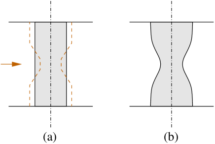
Figure 5: (a) The Gregory-Laflamme instability. (b) A non-uniform black string.

Gregory and Laflamme (GL, 1993 [35]) discovered that the uniform black string solution (5) develops a $z$-dependent metric-instability below a certain critical mass [35] (see figure 5). By a “metric-instability” one means that when one analyzes the spectrum of frequencies-squared for small perturbations around this background, a negative eigenvalue is found.

In hindsight, this instability makes a lot of sense. In general, gravity has a tendency to clump matter. For example, a uniform distribution of gravitating matter (“gas”) is know to be unstable against the formation of inhomogeneities (the so-called “Jeans instability”): when an inhomogeneity forms the denser regions exert a stronger gravitational pull on their neighborhood, thereby triggering an unstable positive feedback. Similarly here, a long enough string “wants” to develop inhomogeneities (if it is short enough then it gets stabilized by the energetic costs of spatial gradients). Another perspective is to recall that the Schwarzschild black hole has negative specific heat (black hole thermodynamics). While this is not enough to de-stabilize a single black hole, it should certainly destabilize a homogeneous collection of black holes, namely a black string, which could increase its entropy by re-distributing its mass non-uniformly. This intuition is the basis for the Gubser-Mitra Correlated Stability Conjecture [36, 37] which states that a homogeneous black brane is (classically) perturbatively unstable if and only if the dimensionally reduced black hole is thermodynamically unstable (semi-classically). From now on we continue to discuss only perturbative instabilities.

The main results of GL are summarized in figure 6 (taken from [35, 39]) which depicts the inverse decay times as a function of $r_{0}/L$ for total spacetime dimensions $5\leq D\leq 10$.

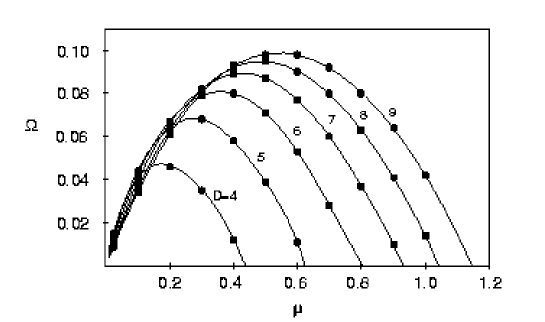
Figure 6: Characteristic inverse decay times $\Omega$ (giving the perturbation an $e^{\Omega\,t}$ time dependence) as a function of the perturbation wavenumber $\mu:=\pi\,r_{0}/L=r_{0}\,k/2$ (proportional to $\mu_{\beta}$ in our notation) for $4\leq D\leq 9$ where $D$ is the extended space-time dimension ($d$ in our notation) in backgrounds with an ${\bf S}^{1}$ compactification. $k_{GL}$, the critical Gregory-Laflamme wave-numbers, are the maximal wavenumbers for which the instability exists – namely, the intersection points with the horizontal axis. The bold points correspond to value calculated numerically and the lines have been traced to guide the eye (all lines converge to the origin $\Omega=\mu=0$ which is a non-physical gauge mode). Reproduced from [35, 39].

From figure 6 we see that the tachyonic mode appears for wavenumbers $k$ (at fixed $r_{0}$) which are lower than a critical wavenumber $k_{GL}$ (which depends on $d$). In order to find $k_{GL}(d)$ it is not necessary to look at perturbations in $D$ dimensions, but rather it suffices to find the negative mode of the Euclidean $d$ dimensional Schwarzschild black hole. This mode, discovered by Gross, Perry and Yaffe [40] (in the 4d case) and hence denoted here by $h_{GPY}$ satisfies

$$L_{Schw}\,h_{GPY}=-\lambda_{GPY}\,h_{GPY}$$ (10)

where $L_{Schw}$ is the Lichnerowicz operator for perturbations in the Schwarzschild background and $-\lambda_{GPY}$ is the negative eigenvalue. Given $h_{GPY}$ the marginally tachyonic mode is given by [41, 38]

$$h=h_{GPY}\,\exp{(i\,k_{GL}\,z)}$$

$$k_{GL}:=\sqrt{\lambda_{GPY}}$$ (11)

In [42] the critical GL lengths were obtained for Schwarzschild black holes in various dimensions (see table 1). From these the high $d$ asymptotic form was extracted and later proven analytically in [17] to be

$$k_{GL}\simeq\sqrt{d}\,{1\over r_{0}}~{}.$$ (12)

This means that for large $d$ the black string becomes unstable at a compactification length $L_{GL}=2\pi/k_{GL}\sim r_{0}/\sqrt{d}$ when it is quite “fat” (namely $r_{0}\gg L_{GL}$) and indicates that such a string would not decay into a black hole which would not “fit” inside the extra dimension.

At $k=k_{GL}$ the GL mode is marginally tachyonic, namely a zero-mode. Morse theory arguments strongly suggest that this zero-mode produces a branch of solutions emanating from the GL point describing non-uniform strings due to the $z$-dependence of the GL mode.

d	4	5	6	7	8	9	10	11
$k_{GL}$	.876	1.27	1.58	1.85	2.09	2.30	2.50	2.69
d	12	13	14	15	19	29	49	99
$k_{GL}$	2.87	3.03	3.19	3.34	3.89	5.06	6.72	9.75

Table 1: Numerically computed static mode wavenumbers $k_{GL}$ in units of $r_{0}^{-1}$ as a function of $d$, the number of extended space-time dimensions [17, 42].

The end-state. Whenever one discovers a perturbative tachyon indicating a decay, the question of its end-state is naturally raised. As the end-state configuration often lies away from the initial configuration a perturbative analysis does not suffice and one needs global information regarding all stable static solutions which is more difficult to obtain.

Gregory and Laflamme believed the end-state to be the black hole, both since that was the only other phase they knew about and since comparing entropies at small $\mu$ one notices that the black hole phase has superior entropy in this regime. Indeed for small $\mu$, where the black hole is well approximated by a $D$ dimensional spherical black hole, the entropies scale as

$$S_{BH}\sim r_{0}^{~{}D-2}\sim\mu^{{D-2\over D-3}}$$

$$S_{St}\sim r_{0}^{~{}d-2}\sim\mu^{{d-2\over d-3}}~{},$$ (13)

in units where $L=G_{d}=G_{D}=1$. It is seen that the exponent $(D-2)/(D-3)=1+1/(D-3)$ is a monotonically decreasing function of its argument and hence the exponent is smaller for $D>d$ (the black hole) resulting in a larger area.

More recently Horowitz and Maeda [43] showed that the black string horizon cannot pinch in finite “horizon time” (namely, finite affine parameter along the horizon generators). They interpreted that as an indication that surprisingly a black hole could not be the end-state of decay and predicted instead the existence of a stable non-uniform string phase that would serve as an end-state. The argument for pinching in infinite horizon time relied on assuming the increasing area theorem for an event horizon and applying it to an area element at the “waist” – the inward collapsing region of the event horizon. The extension to the claim on the end-state involved estimates on why infinite horizon time should imply infinite asymptotic time (time for an asymptotic observer). While these claims stimulated much of the research reported here, and while numerical evidence lends support for “pinching in infinite horizon time” (see subsection 4.3), strong evidence against the end-state being a non-uniform string will be described as this review proceeds, implying that the end-point is actually the black hole phase as originally argued by Gregory and Laflamme (at least in dimension $D\leq 13$). See the summary section for a more complete discussion.

2.3 Issues

Let us formulate some major issues or questions regarding this phase transition. These issues may be roughly divided into two groups: static and time evolution.

The static issues include

• End-state of decay.

• Qualitative form of the phase diagram including the determination of all static phases.

• Detailed quantitative data on the phase diagram: the domain of existence of each phase and the determination of critical points.

During the last couple of years there was significant progress on the static issues, resulting also in the surprising discoveries of critical dimensions and a topology change. The deepest issues belong however to the time evolution

• The spacetime structure, namely determination of the Penrose diagram, or an appropriate generalization thereof.

• A naked singularity and a violation of Cosmic Censorship.

  It is plausible that as the black string pinches a naked singularity is formed, naively because the singularity which “originally” winds the compact dimension gets “broken”, perhaps at the event of pinching. Another argument comes from the clash between the arguments of [43] and results on the system’s phase diagram [44, 34]. Possibilities include a problem with the assumption that there are no singularities strictly outside the horizon and an infinite duration with respect to “horizon-time” (horizon affine parameter) while the asymptotic-time duration is finite. Note that the initial conditions in this case are generic, unlike known examples of naked singularities.

• A thunderbolt and quantum gravity.

  The decay is accompanied by a release of energy (after all, a tachyon is involved) in the form of radiation (see [45]). It is plausible that this radiation pulse is classically singular (a “thunderbolt”), perhaps due to its origin from the naked singularity. In such a case it is quite plausible that some knowledge of quantum gravity will be necessary in order to understand this outgoing radiation.

While there was much progress on the static issues, there was practically none on the time evolution issues, and these remain unsolved.

3 Qualitative features

In order to understand the phase transition physics and to resolve the issue of the end-state it suffices to map out all static and stable solutions of the system, since the end-state is certainly static and stable. But actually, Morse theory arguments will lead us to consider all static solutions whether stable or not, in order to take advantage of a “phase conservation rule” which is a powerful qualitative constraint on the form of the phase diagram. So we seek the phase diagram of all static solutions as a function of $\mu$, and throughout this review we will restrict ourselves to static aspects of the system.

In this section we seek to determine the phase diagram qualitatively, and the quantitative aspects will be described in the next section.

3.1 Order parameter

We wish to define an order parameter ${\hat{\lambda}}$ such that the uniform string will have ${\hat{\lambda}}=0$ and the emerging non-uniform branch (from the GL point) will have ${\hat{\lambda}}\neq 0$, namely ${\hat{\lambda}}$ should be a measure of non-uniformity. Actually, it is desirable to have both the black strings and the black holes at finite values of ${\hat{\lambda}}$, motivated by the expectation for a merger of the two due to Morse theory arguments as will be explained in subsection 3.3.

It turns out that an asymptotic analysis of the metric and the associated charges furnishes physically meaningful candidates [46, 31]. However, it should be noted that the central discussion on the qualitative form of the phase diagram that will culminate in subsection 3.5 will be independent of this choice of the order parameter, and the discussion here is intended mainly to avoid any unnecessary vagueness that tends to lead to concerns, such as the very existence of an appropriate order parameter which is finite on both black-hole and black-string.

For concreteness, we take the compactification manifold to be $X={\bf S}^{1}$ throughout this subsection. Far away from the black object the leading behavior of the radial coordinate $r$ is well-defined (by comparison with the flat geometry) and thus, as usual, it is possible to read the (ADM) mass of the object by the asymptotic $r$ behavior of the metric functions. One such asymptotic constant can be measured from the fall-off of $g_{tt}$ and for a spherical hole in a flat (and topologically trivial) background this would be the only independent asymptotic constant, and it would be proportional to the mass. Here there is one more asymptotic constant: the metric becomes $z$-independent ($z$-dependent modes are massive from the lower dimensional point of view and hence they decay like $\exp(-2\pi n\,r/L),~{}n\in\hbox{Z\kern-3.99994ptZ}$) and thus it is sensible to perform a dimensional reduction asymptotically. After dimensional reduction $g_{zz}$, the size of the extra dimension, turns into a scalar field. Thus we expect two asymptotic charges – the mass and the scalar charge. (The latter is non-conserved, but is conventionally called “a charge”, presumably since it is the coefficient for the leading $1/r^{d-3}$ asymptotic fall-off of a field just like the electric charge can be read from the fall-off of the electro-static potential. It is precisely this property of being the leading term in the asymptotic region which we are interested in.)

One can define the asymptotic charges from either the higher dimensional or from the dimensionally reduced points of view. In the higher dimension the metric defines two asymptotic constants $a,\,b$

$$-g_{tt} = 1-{2\,a\over r^{d-3}}$$

$$g_{zz} = 1+{2\,b\over r^{d-3}}~{}.$$ (14)

From the lower dimension point of view the definition for $b$ conforms with the standard definition of a scalar charge: One defines the scalar field from the $g_{zz}$ component of the metric through $e^{2\,\Phi}:=g_{zz}$, and the scalar charge $\Lambda_{\Phi}$ through the asymptotic behavior of $\Phi$ as $\Phi=\Lambda_{\Phi}/r^{d-3}$ (we are not careful here to fix constants in any particular way). Thus from (14) we see that $\Lambda_{\Phi}\equiv b$.

We identify the total mass from the dimensionally reduced metric which is gotten by a Weyl rescaling of the metric $g_{tt}\to\tilde{g}_{tt}=g_{zz}^{1/(D-3)}\,g_{tt}$ and therefore $\tilde{a}=a-b/(D-3)$, where $\tilde{a}$ is defined by $-\tilde{g}_{tt}=1-2\,\tilde{a}/r^{d-3}$. Identifying $2\,\tilde{a}$ with $r_{0}^{~{}d-3}$ and using (8) we get

$$G_{d}\,M={\Omega_{D-3}\over 8\,\pi}[(D-3)\,a-b]~{}.$$ (15)

In addition to the mass, the asymptotic constants $a,\,b$ can be used to express another physical charge, the tension $\tau$. In a satisfying analogy with the well-known first law of gas thermodynamics

$$dE=T\,dS-P\,dV~{},$$ (16)

where $E,\,T,\,S,\,P,\,V$ are the energy, temperature, entropy, pressure and volume, respectively, $\tau$ is defined here through

$$dM=T\,dS+\tau\,dL~{}.$$ (17)

Namely, the tension is defined to be the thermodynamic conjugate to $L$, the size of the extra dimension (see [47, 48] for earlier and equivalent definitions of tension).

The thermodynamic charges are related to the asymptotic constants $a,\,b$ through

$$\left[\begin{array}[]{c}M\\ \tau\,L\\ \end{array}\right]={\Omega_{D-3}\over 8\pi}\left[\begin{array}[]{cc}D-3&-1\\ 1&-(D-3)\\ \end{array}\right]\,\left[\begin{array}[]{c}a\\ b\\ \end{array}\right]~{}.$$ (18)

This relation may derived either through the thermodynamic definitions or from the “method of equivalent sources”, as we proceed to explain. The thermodynamic definition is fully specified by the gravitational (Gibbons-Hawking) action $I=-\beta F$ where $\beta$ is the inverse temperature and $F$ is the free energy. Alternatively, in the “method of equivalent sources” one imagines that the asymptotic fields were generated by a weak stress-energy source and uses the linearized equations to infer the integrated stress-energy charges from the metric asymptotics. Note that the current expression for the mass (18) coincides with the mass read off the dimensionally reduced metric (15).

Let us gain some insight into the behavior of the tension and the scalar charge. For the uniform string metric (3,4) $b=0$ from its definition (14), and hence $\tau\,L=M/(D-3)$ from (18). For the small black hole, on the other hand, one finds from the Newtonian approximation (83,69) that $\tau=0$ and $b=a/(D-3)$. More precisely, to leading order the tension is proportional to $M^{2}$: $\tau L=(D-3)\,\zeta(D-3)/2~{}(\rho_{0}/L)^{D-3}\,M$ [27, 30]. See table 2 for a summary.

	Uniform string	Small black hole
Scalar charge	0	$G_{d}M/(D-3)$
Tension	$M\,L^{-1}/(D-3)$	0

Table 2: Values for some possible order parameters for both “extreme” phases

Inverting (18) we obtain

$$\left[\begin{array}[]{c}a\\ b\\ \end{array}\right]={8\pi\over\Omega_{D-3}(D-4)\,(D-2)}\left[\begin{array}[]{cc}D-3&-1\\ 1&-(D-3)\\ \end{array}\right]\,\left[\begin{array}[]{c}M\\ \tau\,L\\ \end{array}\right]~{}.$$ (19)

Looking at the expression for the scalar charge $b$ we see that the mass tends to increase it, namely mass “wants to generate more space” for itself, while tension “wants” to contract the extra dimension. Thus we may say that for the uniform string ($b=0$) the tension has exactly the correct value to cancel the tendency of mass to expand the extra dimension.

In fact we empirically find that for all black hole and black string solutions their $b,\,\tau$ parameters lie between the uniform string and the small BH. This is only partly understood. Positive tension $\tau>0$, was proven in analogy with the positive mass theorem [49, 50]. However, it is not clear so far why $b>0$ holds. Actually, when one considers also bubbles (for instance [51]) then $b$ is no longer positive. While $b>0$ would correspond to the bound $\tau\,L/M<1/(D-3)$ it was argued in [46] (see also [52]) that the completely general bound is higher, namely $\tau\,L/M<(D-3)$. This bound is set by the bubble and is consistent with the Strong Energy Condition $T_{00}-1/(D-2)\,T^{\mu}_{\mu}\,g_{00}>0$.

We may now define the order parameter. Since $b$ is zero exactly for the uniform string we can use some multiple of it. The natural choice is a dimensionless scalar charge, being either $b/(G_{d}\,M)$ for the micro-canonical ensemble or $b/\beta^{d-3}$ for the canonical ensemble. The dimensionless scalar charge has the additional advantage of placing all phases at finite values: not only is the uniform string at $b=0$ but also the small black hole is at finite value, namely $b/M=1/(D-3)$, as can be seen from table 2. Alternatively, one may choose a dimensionless tension, such as $\tau/M$, as an order parameter that vanishes not for uniform strings, but rather for black holes, and is closely related to $b$ and $M$ (18).

Here we note that the differential form of the first law of black hole thermodynamics (17) may be integrated using the scale invariance of GR. Namely, when one scales the lengths $L\to e^{\alpha}\,L$ the mass and area (entropy) scale according to $M\to e^{(D-3)\alpha}\,M,\,S\to e^{(D-2)\alpha}\,S$. Taking the differentials for these transformation with respect to $\alpha$ at $\alpha=1$ and substituting into (17) yields

$$(D-3)\,M=(D-2)\,T\,S+\tau\,L~{},$$ (20)

which is a useful formula known as “the integrated first law” or “Smarr’s formula” (shown in the current context in [46, 31]).

An interesting property of a phase diagram with this order parameter is that intersections in the phase diagram are constrained due to the first law [46].

3.2 Order of phase transition

In general, one of the basic properties of any phase transition is its order. In this subsection we first review black hole thermodynamics in the Gibbons-Hawking formalism and the general Landau-Ginzburg theory and then we summarize the results for the system under study.

The gravitational free energy. We will use the standard semi-classical Gibbons-Hawking [53] gravitational free energy given by the gravitational action $I(g_{\mu\nu};\,\beta)=-\beta\,F$ (to be described below) evaluated on a “Euclidean section” of the metric. Since our solutions are static, it is straightforward to obtain a “Euclidean section” simply by taking the transformation $t\to i\,t$. In a standard way, requiring the absence of conical singularities at the horizon fixes the period of Euclidean time to be $\beta=2\pi/\kappa$, where $\kappa$ is the surface gravity which is constant over the horizon by the zeroth law.

The gravitational action $I$ is given by the standard Einstein-Hilbert action with an additional boundary term $I_{\partial}$

$$I=I_{EH}+I_{\partial}$$ (21)

such that $I$ is stationary on solutions with respect to variations of the metric which preserve the boundary metric [53, 54].

$$I_{EH}={1\over 16\pi G}\int_{\cal M}R~{},$$ (22)

where $R$ is the Ricci scalar and $I_{\partial}$ can be defined by either of the following equivalent definitions

• $$8\pi G\,I_{\partial}:=\int_{{\partial}{\cal M}}K$$ (23)

  where $K$ is the trace of the second fundamental form for the embedding of the boundary in the manifold.

• $$8\pi G\,I_{\partial}:={\partial}_{n}V_{\partial},$$ (24)

  the derivative of the boundary $(D-1)$-volume with respect to a (proper length) shift in the normal direction.

• $I_{\partial}$ is the boundary term obtained through integration by parts of $I_{EH}$ such that $I$ contains only first derivatives of the metric and no second derivatives, namely $({\partial}g)({\partial}g)\in I,\,g{\partial}^{2}g\notin I$ where $g$ denotes here a generic metric element.

In asymptotically flat spaces $I_{\partial}$ as defined above (23) diverges and must be regularized. The standard regularization [53] is done by measuring $I$ relative to flat space. One chooses a large cutoff $r=R$, where in our case the boundary is ${\bf S}^{d-2}_{R}\times{\bf S}^{1}_{L(R)}\times{\bf S}^{1}_{\beta(R)}$, where $L(R),\,\beta(R)$ are the periods of the $z,\,t$ directions, respectively. Next one subtract the action of a flat space with the same boundary, which in our case is $\mathbb{R}^{d-1}\times{\bf S}^{1}_{L(r)}\times{\bf S}^{1}_{\beta(R)}$, namely

$$8\pi G\,I_{0}={\partial}_{r}\left.\left(\Omega_{d-2}\,r^{d-2}\,L(R)\,\beta(R)\right)\right|_{R}=(d-2)\,\Omega_{d-2}\,L(R)\,\beta(R)R^{d-3}~{}.$$ (25)

Finally one takes $R\to\infty$.

Combining this with (21,22,23), the free energy $F=F(g_{\mu\nu};\beta)$ is finally given by

$$-\beta\,F=I={1\over 16\,\pi\,G}\int_{\cal M}R+{1\over 8\,\pi\,G}\int_{{\partial}{\cal M}}(K-K_{0})$$ (26)

which includes a bulk integral over $R$, the Ricci scalar and a boundary integral over $K-K_{0}$, where $K$ is the trace of the second fundamental form on the boundary, and $K_{0}$ is the same quantity for the reference flat space geometry.

Landau-Ginzburg theory. In a phase transition some derivative of the free energy is discontinuous and goes through a jump. The order of a phase transition is defined to be the order of this derivative. A first order transition is between two phases which are separated in configuration space and hence have different entropies (and other thermodynamic variables) and are therefore exothermic (involving latent heat) while for second order and higher the phases are continuously connected and there is no finite release of energy.

The Landau-Ginzburg theory of phase transitions [55] tells us how to infer the order of the transition from the local behavior of the free energy near the critical point $F=F(\lambda;\mu)$, where the $\lambda$ variables parameterize (a selected subset of) the configuration space, and may act as order parameters, and the $\mu$ variables are the control parameters, for instance the temperature. In our case, the dimensionless control parameter may be chosen as $\mu\equiv\mu_{\beta}\propto\beta/L$. Geometrically it is the ratio of the two asymptotic periods, while physically it is a dimensionless inverse temperature. Since the control parameter is essentially the temperature, we interpret the thermodynamics as taking place in the canonical ensemble, and accordingly, the name “free energy” is fitting. The relevant configuration variable is $\lambda$, the amplitude of the marginally tachyonic GL mode (11), so symbolically the perturbation is

$$h\sim\lambda\,\exp(i\,k\,z)\,h_{GPY}~{}.$$ (27)

A generic phase transition is of first order as depicted in figure 7. However, in our case $F$ possesses a certain parity symmetry (which is non-generic) which opens the possibility for higher order transitions, as we proceed to explain. We note from (27) that $\lambda$ is complex and its phase is related to translations in the $z$ direction. Since the action is invariant under $z$-translations we have

$$F=F(\mu,|\lambda|^{2})~{},$$ (28)

and the non-uniform phase spontaneously breaks this symmetry. From now on, without loss of generality, we consider $\lambda$ to be real and omit the absolute value notation, so that $F$ is an even function, as claimed. This corresponds to fixing the $z$-translations in (27) through $h\sim\lambda\,\cos(k\,z)\,h_{GPY}$ with a real $\lambda$, and the sign reversal now amounts to shifting $z$ by half a period.

Note that $\lambda$ can be related to the order parameter defined in the previous section, the scalar charge $b$. The latter being invariant under $z$-translations must be a function of $|\lambda|^{2}$ as well. Since they both vanish for the uniform string we conclude that

$$b\propto|\lambda|^{2}$$ (29)

(there is a genericity assumption made here which is confirmed by calculations).

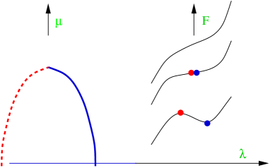
Figure 7: The most generic phase transition – first order resulting from a non-zero cubic term in $F$. On the right we see a sequence of free energy functions, parameterized by $\mu$, with their extrema (phases) highlighted. On the left the phases are extracted into a phase diagram. Stable (unstable) phases are denoted by solid (dashed) lines.

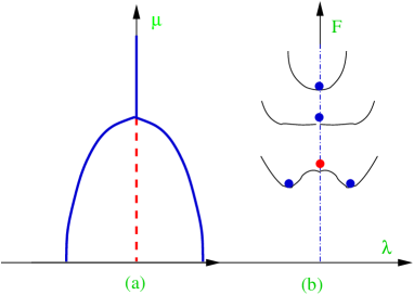
Figure 8: For an even free energy the order of transition could be first or higher depending on a sign. This figure shows a second order transition (or higher) since the free energy has a minimum at the critical point. Same conventions as in figure 7.

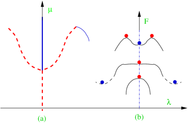
Figure 9: An even free energy results in a first order transition if it has a maximum (or more precisely a non-minimum) at the critical point. Same conventions as in figure 7.

Having a marginally tachyonic mode appear at some critical value $\mu_{c}$ means that the quadratic term in $\lambda$ has a zero at $\mu_{c}$, namely

$$F=F_{1}\,(\mu-\mu_{c})\,\lambda^{2}+\dots$$ (30)

where $F_{1}$ is some positive constant (assuming the phase is stable for $\mu>\mu_{c}$ as is our case). Now the Landau-Ginzburg theory suggests to expand the free energy at $\mu_{c}$ to higher orders in $\lambda$ and to test whether the free energy has a minimum or not. If $F$ has a minimum at $\mu_{c}$, as in figure 8, then for $\mu<\mu_{c}$ two stable minima are created close by at small $\lambda$, the system will continuously evolve into these new phases and the transition must be second order (or higher). If however $F$ has a “direction of descent” at $\mu_{c}$, as in figure 9, that means that since $F$ must be bounded from below there must be some other minimum at some finite value of $\lambda$, whose free energy is lower than the $\lambda=0$ phase. Therefore the system underwent already a first order transition at some higher value of $\mu$ where the free energies of both phases were equal.

Therefore Landau-Ginzburg theory instructs us (in our case, where $F$ is even) to expand

$$F=F_{1}\,(\mu-\mu_{c})\,\lambda^{2}+F_{2}\,\lambda^{4}+\dots$$ (31)

and to determine the sign of $F_{2}$, the quartic coefficient at $\mu_{c}$. Positive (negative) $F_{2}$ implies a second (first) order transition. Of course if $F_{2}$ happens to vanish one needs to compute higher orders, but this did not happen in this system.

Actually, so far we neglected all other modes except for the GL mode. When these are brought into consideration one finds it is required to compute first the (quadratic) back-reaction of the GL mode and incorporate it into the computation of the quartic term in the action. The reason for taking the back-reaction is that what we really want to know is whether the emergent phase from the critical point goes up or down in $\mu$ in the phase diagram, indicating a first or second order transition. To see that we denote the extra modes by $y^{i}$ and expand the free energy as follows

$$F(\lambda,y^{i};\mu)=F_{1}\,(\mu-\mu_{c})\,\lambda^{2}+F_{2\lambda}\,\lambda^{4}+F_{2i}\,\lambda^{2}y^{i}+K_{ij}\,y^{i}\,y^{j}+\dots$$ (32)

The equation of motion for the $y^{i}$ is $0={d\over dy^{i}}F=2K_{ij}y^{j}+F_{2i}\,\lambda^{2}=0$. We denote the solution by $y^{i}=\lambda^{2}\,B^{i}$, where $B^{i}$ stands for back-reaction. The equation of motion for $\lambda$ is $0={d\over d\lambda}F=2\,F_{1}\,(\mu-\mu_{c})\,\lambda+4\,F_{2\lambda}\,\lambda^{3}+2\,F_{2i}\,\lambda y^{i}$. After diving by $\lambda$ and using the equations of motion for $y^{i}$ we find that $-2F_{1}(\mu-\mu_{c})=4\lambda^{2}\left(F_{2\lambda}-K_{ij}\,B^{i}\,B^{j}\right).$ Namely, in order to determine $\mbox{sgn}(\mu-\mu_{c})$ and from that the order of the transition we need to compute

$$F_{2}:=F_{2\lambda}-K_{ij}\,B^{i}\,B^{j}$$ (33)

where $B^{i}$ is the back-reaction that solves the $y^{i}$ equations of motion. Note that $F_{2}$ is computed without deviating from criticality $\mu=\mu_{c}$.

Results. The determination of the order was first carried out by Gubser [56] for the background $\mathbb{R}^{3,1}\times{\bf S}^{1}$ (see also Wiseman’s improvement [57]). Part of the original motivation there was to find a second order phase transition and hence together with it a branch of stable non-uniform strings emanating from the GL point, such as those predicted by [43]. However, the transition was found to be first order. Sorkin [42] generalized the method to the backgrounds $\mathbb{R}^{D-2,1}\times{\bf S}^{1}$ and found a surprising critical dimension

$D\leq 13$ first order $D\geq 14$ second order  .

The critical dimension $D^{*}=``13.5"$ is demonstrated in figure 10. Kudoh and Miyamoto [58] observed that the critical dimension depends on the ensemble: Sorkin’s critical dimension holds for the micro-canonical ensemble, while in the canonical ensemble the critical dimension is lower by one. In subsection 6.1, “results”, we comment on the relation of these results with the predictions of [43].

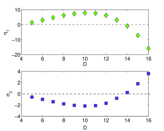
Figure 10: The first correction to the mass $\eta_{1}$ and to entropy (relative to a uniform string with the same mass) $\sigma_{2}$ for the non-uniform string branch emanating from the GL point for backgrounds $\mathbb{R}^{D-2,1}\times{\bf S}^{1}$ – see [42] for precise definitions. From our general discussion we know that there is only one sign to be determined (that of $F_{2}$), and indeed the signs of $\eta_{1},\,\sigma_{2}$ are correlated. At the critical dimension $D^{*}=13.5$ there is a change of sign indicating the transition becomes second order for higher $D$. Adapted with permission from [42].

Due to the importance of the critical dimension it is a good idea to develop some intuition about it. First, as discussed around equation (12) for high $D$ the critical GL string is quite “fat” and we expect that the string will not decay (directly) into the black hole, which would be “too big to fit” inside the extra dimension (see also [59] for a similar argument involving $\mu_{S}$, which is defined below). Another indicator comes from comparing $\mu_{GL}$ with $\mu_{S}$ the value of the approximate equal area point: $S_{St}(\mu_{S})=S_{BH}(\mu_{S})$ where $S_{St}$ is the entropy of the uniform string and $S_{BH}$ is BH area approximated by the small black hole expression. For a first order transition we expect $\mu_{S}>\mu_{GL}$ but that holds only for $D<12.5$.

Method. Gubser’s method [56] was to perturbatively follow the branch of non-uniform strings emanating from the GL critical point. The perturbation parameter is $\lambda$, the amplitude for the GL mode (27), and in order to determine the order of the transition is was necessary to compute some metric functions up to the third order in the perturbation parameter. As we mentioned above, to determine the order there is a somewhat more efficient method, namely it is actually enough to compute only the second order back-reaction and substitute into the quartic part of the action (see appendix A in [44] and [18]). However, the longer computation naturally yields additional results not included in the shorter one.

In practice, when computing the back-reaction we consider a continuum of modes, and therefore the discrete index $i$ in (32) and the discussion around it is replaced by the continuous variable $r$, and the “field”$y$ is replaced by the all the fields in the problem. Moreover, inverting the linear operator $K$ to solve for $y$ means obtaining the fields by solving a second order ODE (obtained from linearizing the equations of motion) with a source term quadratic in the perturbation (the first order mode).

3.3 Morse theory

When one turns to consider the question of the end-point for decay, or more generally of finding the phase diagram of all static phases, one is at first discouraged by the lack of any knowledge regarding the non-uniform strings and the big black holes. The most interesting question is to determine the qualitative features of the phase diagram. For that purpose one needs qualitative tools, and one such tool was given in [44] under the name “Morse theory”, fulfilling the intuition that generically a phase persists as the system is “deformed” by changing a parameter, and that the disappearance of a phase should require some special circumstances that are worth elucidating.

Indeed solutions of the Einstein equations are extrema of the gravitational action in the space of metrics, and as such are generically stable under perturbations. The topological theory of extrema of functions is well-known and is called “Morse theory” and it includes the specification of the allowed transitions.

For other qualitative tools in the study of thermodynamics in the astrophysical context of self-gravitating systems see the review [60], and especially the closely related Poincaré method to determine the perturbative stability of phases just by looking at a certain kind of a phase diagram.

Actually, there is a subtlety in the identification of extrema of the action with solutions of the equations of motion due to gauge (diffeomorphism) redundancy, which we would like to mention. It is certainly true that solutions are extrema of the action. However we wish to consider the action as a function of metrics up to gauge invariance, namely as a function of the gauge-fixed metric. Therefore the extremum equations should be supplemented by the gauge-fixing constraints. Nevertheless, in this case it was found [57] that the constraints are actually implied by the extremum requirement through a combination of properly chosen boundary conditions and the constraints’ Bianchi identities. It could be that this is true more generally.

A lightning review of Morse theory (see section (3.2) of [44] for a somewhat longer introduction). For functions of one variable the ways in which an extrema can disappear are clear

• Annihilation. A maximum and a minimum can coalesce under continuous deformation and disappear into a monotonous function. We call this the basic 1d vertex of “annihilation” – see figure 7.

• Run-away. An extrema of a function $f(x)$ may run away to infinity either in $x$ or in $f$ during a finite range of deformation parameter. In this paper we shall find “annihilation” explanations for changing phases, and thus we will not need to resort to “run-away” explanations, even though they are certainly a logical possibility.

When one considers a function of several variables, $f=f(\vec{x})$, one may get a simple generalization of the basic 1d vertex by adding $n$ spectating negative directions as well as $N-n-1$ positive directions, namely $f(\vec{x})=f_{0}(x_{0};\mu)-\sum_{i=1}^{n}f_{i}\,x_{i}^{~{}2}+\sum_{j=n+1}^{N-1}f_{j}\,x_{j}^{~{}2}$, where $f_{0}(x_{0};\mu)$ is a 1d function such as the one depicted in figure 7, and $f_{i},~{}1\leq i\leq N-1$ are positive constants. Now, the minimum in figure 7 turns into an extremum with $n$ negative modes, while the maximum has $n+1$ negative directions. Therefore we obtain, what we call “the basic vertex”

Basic vertex: two extrema with $n$ and $n+1$ negative directions may annihilate.

While for generic extrema the Hessian is non-degenerate and $n$ is well-defined, one may wish to know the rules for more general vertices. Indeed, Morse theory can be phrased as saying that the most general vertex is a coincidence of several of these basic vertices, thereby justifying our use of the adjective “basic”.

The conclusion and some reservations. We see that a stable phase ($n=0$) is allowed to disappear at the expense of “annihilating” with an unstable phase with one negative mode ($n=1$). The latter in turn can disappear by annihilating against either $n=0$ or $n=2$ phases and so one. This is exactly the “phase conservation rule” [44] which we were seeking. It sets a strong qualitative constraint on the existence of phases. However, the price to be paid is that all phases must now be mapped out, not only the stable ones.

As shown in figures 8,9 this rule determines the stability of the non-uniform string emanating from the GL point. One may ask where this phase might end. From the phase conservation rule we conclude that the simplest way to satisfy it, without requiring any additional phases, is that the non-uniform string phase would annihilate against the black hole phase [44] at a point on the phase diagram that we call “the merger”. Taking into account the existence of a critical dimension we find that depending on the dimension we get two possible behaviors: for $5\leq D<D^{*}$ the non-uniform black string, which is unstable for small non-uniformity, annihilates with the black hole (which is stable when it is small) while for $D>D^{*}$ a stable non-uniform string transforms into a stable BH, and $D^{*}=12.5$ ($13.5$) in the canonical (micro-canonical ensemble). This is our main conclusion from Morse theory and we stress again that it seems to be the simplest scenario, but others cannot be excluded.

The rigor of the prediction of a phase merger, even if intuitive and clear, is questionable due to the following observation. In the next section we will see that the Euclidean versions of the black hole and the string have different topologies and hence their metrics would be expected to live in different, disconnected spaces of metrics, and it wouldn’t make sense for phases to move from one space to the other. Nevertheless, we shall take the prediction above seriously and look whether these two spaces of metrics are in some sense glued together. Indeed we shall find a continuous transition (and in finite distance) between the two spaces, which we view as an important confirmation for the consistency of the picture. However, the way in which the spaces are glued is still poorly understood, and the gluing may very well be non-smooth as well as involve the infinite dimensionality of the space of metrics in an essential way, in which case the validity of the Morse theory argument is not self-evident. At this point, I consider the conclusion above to be essentially correct and justified if not rigorously a priori then a posteriori by the agreement of the predicted and the numerically computed phase diagrams.

An example: the Hawking-Page transition. The reader familiar with the phase transition between thermal Anti-de-Sitter (AdS) and large black holes in AdS, known as the “Hawking-Page transition” [61], may benefit from applying the Morse theory ideas above to that context.

In the Hawking-Page transition in its canonical ensemble setting, one considers a space-time with a negative cosmological constant $\Lambda$ whose boundary is that same as that of thermal AdS, namely a large spatial sphere of Radius $R$ times a compact circle of Euclidean time of size $\beta\,\sqrt{-\Lambda}\,R$. The dimensionless control parameter is $\beta_{\Lambda}:=\beta\,\sqrt{-\Lambda}$, and as usual $\beta/\hbar$ is the inverse temperature. In 4d Hawking and Page found that several phases exist in this system as follows. For $\beta_{\Lambda}>\beta_{0}={1\over 2\,\pi}$ the only phase which exists is thermal AdS, AdS filled with a thermal gas of radiation. For $\beta_{0}>\beta_{\Lambda}>\beta_{1}={1\over\sqrt{3}\,\pi}$ two additional phases show up, the small and large AdS black holes (inside a thermal bath), the large (small) black hole being thermodynamically stable (unstable) due to its positive (negative) specific heat. However, the black holes’ free energy is inferior to that of thermal AdS. Finally at $\beta_{\Lambda}<\beta_{1}$ the large black hole dominates.

In the current context, this phase transition, which is a first order phase transition is described in figure 11 (compare with the general first order transition of figure 7). For $\beta>\beta_{0}$ there is a single minimum for the free energy which is thermal AdS. At $\beta=\beta_{0}$ two phases are “pair created” (or “annihilated” if one approached $\beta_{0}$ from below) through our “basic vertex”: a stable large black hole and an unstable small black hole, but thermal AdS still has lower free energy. Here we are assuming the Gubser-Mitra Correlated Stability Conjecture [36, 37] to infer the perturbative stability or instability from the sign of the specific heat and the associated thermodynamic stability of the black holes. Then at $\beta=\beta_{1}$ a first order phase transition occurs when the free energies of thermal AdS and the large BH become equal. Finally, for smaller $\beta$ the large BH dominates.

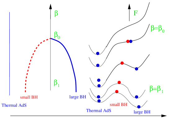
Figure 11: The free energy and phase diagram for the Hawking-Page transition [61] in AdS space, which is a first order phase transition. At $\beta=\beta_{0}$ the unstable small black hole phase meets the stable large black hole phase and they “annihilate” according to our ”basic vertex” rule.

3.4 Merger point

In the last subsection we saw how Morse theory makes it plausible that the non-uniform string phase merges with the BH phase. We shall first encounter a problem for this picture, namely topological differences between the two phases. However, we are familiar with some topology changes such as the flop and the conifold, and one of the surprising results of the research on this system is the emergence of a novel type of topology change, called the “merger” transition in [44].

A topology change. Intuitively the transition from black string to black hole involves a region where the horizon becomes thinner and thinner as a parameter is changed until it pinches and the horizon topology changes. We call this region “the waist” and this process is described in the upper row of figure 12 using the $(r,z)$ coordinates defined in figure 2. It is important to remember that all metrics under consideration are static and that they change as we change an external parameter, not time. Since the metrics are static we may as well consider their Euclidean versions (this point was discussed in the second paragraph of section 3.2).

We shall now demonstrate that this merger transition involves a local topology change of the Euclidean manifold. Let us zoom in around a very thin waist, whereby all the scales of the problem such as $GM$ and $L$ are very large and irrelevant, identifying what may be called the local geometry at the waist. Consider a co-dimension 1 surface within the local geometry but far away from the waist, such as the one denoted by a dashed line in all three geometries in the top row of figure 12. Actually, this surface is the asymptotic boundary of the local geometry.

The topology of this asymptotic boundary is given by ${\bf S}^{D-3}_{\theta}\times{\bf S}^{2}_{r,z,t}$ as we proceed to explain. The angular piece, ${\bf S}^{D-3}_{\theta}$, is obvious while the ${\bf S}^{2}_{r,z,t}$ requires explanation. One should remember that in our figures, such as figure 12, we suppress not only the angular coordinates but also the time variable. In the Euclidean continuation the Euclidean time must be periodic in order to avoid a conical singularity at the horizon, and moreover, the proper size of this circle vanishes at the horizon ($g_{tt}=0$ at the horizon). Thus the circle fibration of Euclidean time over an interval (the dashed line in figure 12), such that the fibred circle shrinks on the edges exactly produces a topological ${\bf S}^{2}$. This is just like the fibration of the surface of the earth by latitude lines, which shrink at the poles (see figure 13).

Naturally, the topology of this boundary surface is constant as local changes occur near the waist. Next we notice that in the black-hole phase the ${\bf S}^{D-3}_{\theta}$ is contractible (onto the exposed $r=0$ axis), while in the string phase the ${\bf S}^{2}_{r,z,t}$ is contractible. Therefore the local topology of (Euclidean) spacetime is changing, not only the horizon topology. Thus, the topology change can be modelled by a “pyramid” (just like the conifold transition) – see the lower row of figure 12: the rectangular basis of the pyramid denotes the asymptotic boundary ${\bf S}^{D-3}_{\theta}\times{\bf S}^{2}_{r,z,t}$ where each edge represents one of the sphere factors, and the pyramid’s truncated apex encodes which one of the spheres is contractible and which one remains of finite size and is non-contractible. By the nature of topology, in order to change it there must be at least one singular solution along the way (with at least one singular point). The simplest possibility, (which is also realized in the conifold) is to assume that the the singular geometry is the cone over ${\bf S}^{D-3}\times{\bf S}^{2}$.

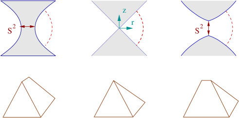
Figure 12: The merger transition. Shaded regions are inside the horizon and the dashed line is a boundary far away. The singular configuration is a cone over ${\bf S}^{2}\times{\bf S}^{2}$.

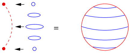
Figure 13: An illustration of the fibration of an ${\bf S}^{2}$: circles fibred over an interval such that the fiber shrinks at the edges (left) are equivalent to a surface of a sphere (right). In this way the dashed intervals in the top row of figure 12 actually represent spheres, once the circles of Euclidean time are taken into account.

It is suggestive that the local space-time topology change is also accompanied by a change in the global topology. I believe this is the case for the following reason. The black string solution is contractible to ${\bf S}^{D-3}_{\theta}\times{\bf S}^{1}_{z}$ (after contracting the $r,t$ cigar), and thus its elementary non-contractible cycles are ${\bf S}^{D-3}_{\theta}$ and ${\bf S}^{1}$. For the black hole on the other hand the non-contractible cycles seem to be ${\bf S}^{D-2}_{\chi\theta},\,{\bf S}^{2}_{z,t}$ and ${\bf S}^{1}_{z}$: the ${\bf S}^{D-2}_{\chi\theta}$ is the horizon, the ${\bf S}^{1}_{z}$ is the compact $z$ direction and the ${\bf S}^{2}_{z,t}$ is the $r=0$ axis connecting the poles together with the time fibration. It is seen that there are several topological differences between the geometries, for instance, the black hole has a 2d topologically non-trivial cycle while the string does not.

Cones. Figure 12 encodes the topological nature of the merger. But is it really true that this can be realized with Ricci-flat metrics?

It is easy to write down a Ricci flat metric for the singular solution, the cone (see the middle of figure 12). Actually this can be done for a somewhat more general cone, the cone over ${\bf S}^{m}\times{\bf S}^{n}$ with no additional “cost”. The metric is

$$ds^{2}=d\rho^{2}+{\rho^{2}\over D-2}\left[(m-1)\,d\Omega^{2}_{{\bf S}^{m}}+(n-1)\,d\Omega^{2}_{{\bf S}^{n}}\right]~{},$$ (34)

where the $\rho$ coordinate measures the distance from the tip of the cone, $D=m+n+1$ is as usual the total spacetime dimension and the constant pre-factors are essential for Ricci-flatness. Note that $\rho=0$ is the singular tip of the cone, unless $m=0$ (or $n=0$) when it becomes the smooth origin of $\mathbb{R}^{D}$ in spherical coordinates.

In order to exhibit “smooth cone” metrics which approach the singular cone from both sides of the transition (see right and left portions of figure 12) one may use the following ansatz

$$ds^{2}=d\rho^{2}+e^{2\,a(\rho)}\,d\Omega^{2}_{{\bf S}^{m}}+e^{2\,b(\rho)}\,d\Omega^{2}_{{\bf S}^{n}}$$ (35)

with boundary conditions at $\rho\to 0$

$$a(\rho=0) = a_{0}$$

$$b(\rho) = \log(\rho)$$ (36)

such that ${\bf S}^{m}$ becomes non-contractible while ${\bf S}^{n}$ joins with $\rho$ to make a smooth neighborhood of the origin of $\mathbb{R}^{n+1}$.

Using (92) for the Ricci scalar of a fibration and after integration by parts one gets the action for $a,b$

$$S={\Omega_{m}\,\Omega_{n}\over 16\,\pi\,G_{D}}\int d\rho\,e^{m\,a+n\,b}\,\left[m(m-1)\,(a^{\prime 2}+e^{-2\,a})+n(n-1)\,(b^{\prime 2}+e^{-2\,b})+2\,m\,n\,a^{\prime}\,b^{\prime}\right]~{}~{}.$$ (37)

Einstein’s equations are

$$a^{\prime\prime} = (m-1)\,e^{-2\,a}-m\,a^{\prime~{}2}-n\,a^{\prime}\,b^{\prime}$$

$$b^{\prime\prime} = (n-1)\,e^{-2\,b}-n\,b^{\prime~{}2}-m\,a^{\prime}\,b^{\prime}$$

$$0 = m\,(a^{\prime~{}2}+a^{\prime\prime})+n\,(b^{\prime~{}2}+b^{\prime\prime}).$$ (38)

These equations are very similar to the equations encountered in the Belinskii-Khalatnikov-Lifshitz (BKL) analysis of the approach to a space-like singularity (see the recent excellent “Cosmological Billiard” review [1]). Although the general (and often singular) qualitative behavior of these equations as $\rho\to 0$ for arbitrary initial conditions was not obtained in [44], it was checked that for the boundary condition (36) $a(\rho),\,b(\rho)-\log(\rho)$ can be expanded in a Taylor series around $\rho=0$ and the recurrence equations for the Taylor coefficients could be solved without encountering an obstruction.

Once a single smoothed cone solution is available, constructing a full family that approaches the singular cone is a matter of simply rescaling it. As illustrated in figure 14, since away from the smoothed tip the smoothed cone asymptotes to a cone, a geometry which is scale invariant, then after rescaling there is a natural way to identify the asymptotic cones, thereby specifying the way to take the limit over the family of rescaled metrics.

Altogether we succeeded in realizing the local topology change encoded in figure 12 by a family of Ricci-flat metrics. I consider this non-trivial property to be strong evidence for the merger picture as presented in subsection 3.3.

Figure 14: A single smoothed cone solution can be scaled down to provide a continuous family of metrics which approach the cone.

I would like to stress some of the assumptions involved in locally modelling by cones

• The singular solution has a single singular point.

• The singular solution is continuously self similar (CSS).

Both assumptions are reasonable and minimal: there could be more than a single singularity, but there is at least one, and the local singular solution must forget the “long distance” scales and hence it would be scale-free, and the simplest way to obtain that is if the solution is self-similar. Continuous self-similarity would be the simplest possibility and in [44] it was found to lead to a local isometry enhancement where the $\chi$ coordinate (see figure 2) conspires with $t$ to make a round ${\bf S}^{2}$. Indeed, a Numeric study [62], limited by numerical resolution, found consistent evidence for this cone structure. More recently it was claimed in [63] that in a certain range of dimensions ($5\leq D<10$) continuous self-similarity (CSS) is in fact (spontaneously) broken into discrete self-similarity (DSS) which requires to replace the cones by certain “wiggly cones” as local models of the merger point.

Tachyons on cones. It turns out that the cones may have tachyons and that their existence surprisingly depends on a critical dimension $D^{*}_{\mbox{merger}}=10$ as we proceed to show – see also [44] and references therein including [64].

The dangerous mode is a function $\epsilon(\rho)$ which inflates slightly one of the spheres while shrinking the other. The ansatz for the perturbation is

$$ds^{2}=d\rho^{2}+{\rho^{2}\over D-2}\left((m-1)\,e^{2\,\epsilon/m}\,d\Omega^{2}_{{\bf S}^{m}}+(n-1)\,e^{-2\,\epsilon/n}\,d\Omega^{2}_{{\bf S}^{n}}\right)~{}.$$ (39)

A priori one could start with two separate scale functions, one for each sphere, but the $G_{\rho\rho}=0$ constraint relates them as above (after ignoring the trivial perturbation which represents $\rho$-translation) – for more details see [44] eq. (6.6) and below.

The quadratic part of the action, disregarding an overall constant is

$$I\sim\int\rho^{D-1}\,d\rho\left[{2\,(D-2)\over\rho^{2}}\,\epsilon^{2}-\epsilon^{\prime~{}2}\right]~{},$$ (40)

and through the change of variables ${\hat{\rho}}^{-1}=(D-2)\,\rho^{D-2}$ it can be recast to have a canonical kinetic term

$$I\sim\int d{\hat{\rho}}\left[{2\over(D-2)\,{\hat{\rho}}^{2}}\,\epsilon^{2}-\epsilon^{\prime~{}2}\right]~{}.$$ (41)

The equation of motion for $\epsilon$, namely the zero mode equation, is

$$[-\hat{{\partial}}^{2}+V({\hat{\rho}}) ] \epsilon=0$$ (42)

$$V({\hat{\rho}}) = -{2\over(D-2)\,{\hat{\rho}}^{2}}~{},$$ (43)

The solutions are

$$\epsilon = \rho^{s_{1,2}}$$

$$s_{1,2} = {D-2\over 2}\,\left(-1\pm i\sqrt{{8\over D-2}-1}\right)~{}.$$ (44)

The expression (44) for $s_{1,2}$, the characteristic exponents, reveals a critical dimension [44]

$$D^{*}=10$$ (45)

such that for $D<D^{*}$ $s$ are complex while for $D>D^{*}$ they are real. Complex characteristic exponents (for $D<D^{*}$) imply that (the real part of) the zero mode has infinitely many nodes (zeroes) equally spaced in $\log(\rho)$ with “log-period” $\Delta_{e}=2\pi/\Im(s)$. The presence of infinitely many nodes for the zero mode implies the presence of infinitely many tachyons, just like the number of nodes of the zero-energy solution to a Schrödinger equation counts the number of negative energy states. In [63] these log-periodicity and tachyons (for $D<D^{*}$) were interpreted as an indication for a spontaneous breaking of continuous self-similarity (CSS) into discrete self-similarity (DSS). For $D>D^{*}$ on the other hand, $\Im(s)=0$ and there are no nodes nor tachyons.

Note that $D^{*}$ is the total spacetime dimension, and it is independent of $m$ and $n$ separately. When we wish to distinguish this critical dimension from others we shall denote it by $D^{*}_{\mbox{merger}}$.

One can view the zero-mode equation (42) in a wider context by considering the eigenvalue problem

$$[-\hat{{\partial}}^{2}+V({\hat{\rho}})]\epsilon=\lambda\epsilon$$ (46)

where $V$ is the same as in eq. (43), $\lambda$ is the eigenvalue, and we note that (46) reduces to (42) upon setting $\lambda=0$.

The eigenvalue problem (46) is in Schrödinger form, and we may apply known results. For potentials of the general form $V=-c/r^{\alpha}$ it is well-known that while the classical energy is unbounded from below, the quantum problem may have a ground state as long as the potential is not “too negative”. For instance, for $\alpha=1$ we get the Hydrogen atom. More generally the spectrum is bounded from below for $\alpha<2$, while for the critical value $\alpha=2$, which is our concern here, the prefactor $c$ becomes dimensionless and the potential is conformally invariant. Due to scale invariance the spectrum is constrained to be invariant under positive rescaling of the eigenvalues. Now $c$ itself exhibits a critical value, namely $c^{*}=1/4$, such that the spectrum is bounded from below and actually non-negative only for $c\leq c^{*}$ (since the $E=0$ solution has no nodes – see for example [65]). Equating $2/(D-2)=c^{*}=1/4$ we arrive once more at $D^{*}=10$ as in (45).

Some moduli space properties. The merger transition lies in finite distance in moduli space (actually, it would not deserve to be called a “topology change” otherwise, since it would require infinite “resources” to be reached.) The argument was unpublished so far and here it is supplemented as appendix B. Moreover, the appearance of a kink in the phase diagram at merger was predicted in section (5.3) of [44], and the numerics indeed seem to exhibit some sort of a kink – see the next section.

3.5 Phase diagrams – predictions and data

We may now assemble all the theoretical input and draw the predicted qualitative form of the phase diagram for various spacetime dimensions – see figure 15. These figures apply with small changes to both the micro-canonical ensemble, which is the usual physical setting where energy is conserved, and to the canonical ensemble, namely black holes immersed in a heat bath.

The vertical axis is the dimensionless control parameter $\mu$ defined by either the dimensionless mass $\mu_{M}$ (1) in the micro-canonical ensemble or by the dimensionless inverse temperature $\mu_{\beta}$ (2) in the canonical. The horizontal axis is the order parameter chosen in subsection 3.1 to be the dimensionless scalar charge (see especially eq. (14) and the next to last paragraph in that subsection).

The local structure around the GL point is determined by the order of the transition as discussed in subsection 3.2: for $D<D^{*}$ the GL vertex is first order [56] just like figure 9, while for $D>D^{*}$ it is a second order vertex just like figure 8. $D^{*}$, the critical dimension depends on the ensemble – in the micro-canonical case it is $D^{*}=``13.5"$ [42] while in the canonical case it is $D^{*}=``12.5"$ [58].

Finally, we connect the black hole and black string phases, as suggested by the central conclusion of subsection 3.3, based on Morse theory arguments and further justified by presenting a novel topology change in subsection 3.4.

The diagrams in figure 15 were constructed by attempting to draw the simplest diagram consistent with the data and assumptions in the last two paragraphs. The non-trivial nature of these diagrams is best illustrated by the various other possibilities that were considered in the literature, see for example the six scenarios in [66], section 6.

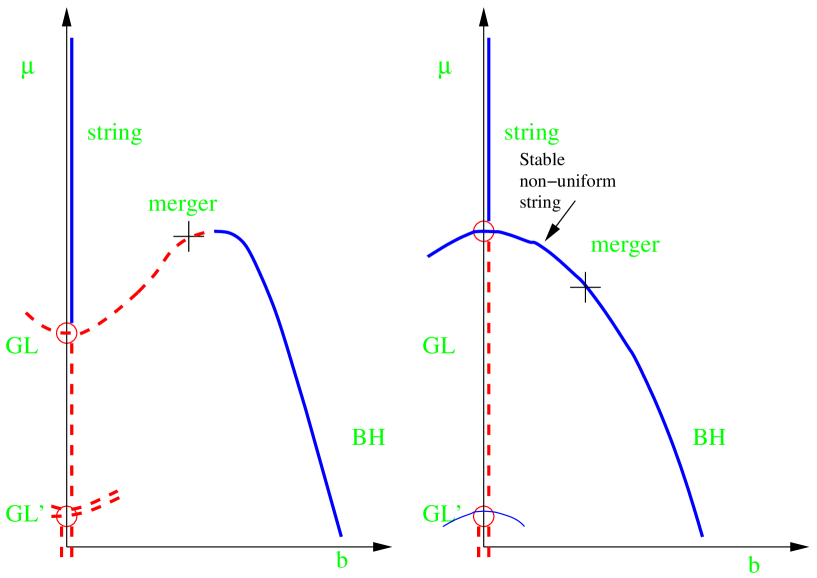
$5\leq D<D^{*}$                                      $D>D^{*}$

Figure 15: The predicted qualitative form of the phase diagram. The vertical axis is the control parameter $\mu$ and the horizontal axis is the dimensionless scalar charge, which plays the role of the order parameter (see the text for further detail). Solid (blue) lines denote stable phases and dashed (red) lines denote unstable phases. The “+” denotes the merger point where the black-hole and black-string phases meet in a topology changing transition (of the Euclidean solutions). Note the dimensional dependence of the qualitative form due to the critical dimension. The diagram on the left basically appeared in [44].

The critical dimension $D^{*}_{\mbox{merger}}=10$ (45) affecting the stability of the ${\bf S}^{m}\times{\bf S}^{n}$ cone in the critical merger solution is not visible in figure 15. According to the picture that emerges from [63], there is a single branch of non-uniform strings, irrespective of $D^{*}_{\mbox{merger}}$ (and being unstable as long as the transition is first order), but for $D<10$ this solution approaches a discretely self-similar (DSS) solution near the singularity, while for $D>10$ it approaches a continuously self-similar (CSS) solution there. While the qualitative predicted form is similar, the kink at merger is likely to be different.

Another point to note is the critical point GL’ in figure 15 which is there to remind us that each (non-uniform) solution has “harmonies” or “copies” gotten by trivially fitting several cycles inside $L$, namely replacing $L\to L/m$ for any $m\in\hbox{Z\kern-3.99994ptZ}_{+}$ in the solutions. In particular the GL point has these copies. However, these copies of the phase diagram are decoupled (except for their connection with the uniform string) and therefore there is no need to draw them. See also [66].

Numerical data. Clearly, the predicted phase diagrams in figure 15, were not proven here, but rather argued to be the simplest possibility which is consistent with certain carefully analyzed arguments, some of them not fully understood yet. As such it suggests to be tested by actually obtaining these solutions. Indeed, one of the joys of this problem is the feedback between theory and numerics, which is in many ways like the classical feedback between experiment and theory which we sorely miss.

Recently the numerical determination of the phase diagram in 6d was all but completed [34] – see figure 16. A visualization of the merger transition through embedding diagrams is shown in figure 17.

We see perfect agreement with the predicted diagram in figure 15 with $D=6$ (which basically appeared already in [44]), especially regarding the prediction for a “merger” of the black hole and the string phases, and the absence of a stable non-uniform phase (predicted by [43]). We view this as a vindication of the picture presented here. Additional interesting features of the numeric figure are a kink at merger, perhaps related to the predicted kink (see the last paragraph in the previous subsection), and the location of the merger at roughly a local maximum on the diagram.

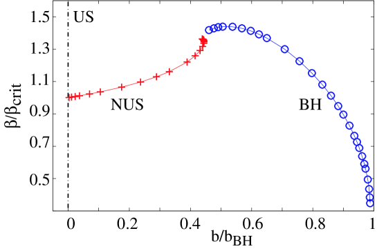
Figure 16: Numerical data for the phase diagram in 6d. “US”’ denotes the uniform string branch, “NUS” denotes the non-uniform string branch (data from [57]) and “BH” is the black hole (data from [34]). Axes conventions are the same as in figure 15 (vertical is $\mu_{\beta}$ and the scalar charge is in units of mass rather than temperature). Adapted with permission from [34].

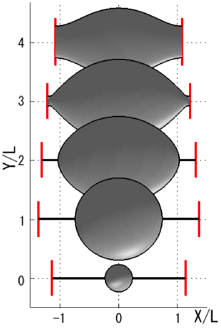
Figure 17: Embedding diagrams for a sequence of event horizons in 6d, starting with non-uniform strings (top, data from [57]) and passing through the merger transition to black holes (bottom, data from [34]). $X$ is the compact dimension and $Y$ is the radial direction. Note that although the asymptotic size of the extra dimension, $L$, is kept fixed, the “proper” size (for embedding purposes) changes. Reproduced with permission from [34].

These diagrams were obtained by combining data from two different simulations - one for non-uniform strings [57] and one for the black holes [34], see also [32, 33] for previous work. More details on the challenges overcome in performing these simulations appear in the next section.

4 Obtaining solutions

In the previous section we examined the qualitative features of the phase diagram. Now we turn to the more quantitative aspects, those required in order to obtain solutions for static black objects.

4.1 2d gravito-statics

Counting degrees of freedom. The most general metric which is static and spherically symmetric is

$$ds^{2}=e^{2\,A}\,dt^{2}+ds^{2}_{(r,z)}+e^{2\,C}d\Omega^{2}_{D-3}~{},$$ (47)

where all functions are defined on the $(r,z)$ plane, $ds^{2}_{(r,z)}$ is an arbitrary metric on the plane and since the metrics are static we might as well work with Euclidean signature.

Altogether the problem is defined in the 2d $(r,z)$ plane and the field content is the metric and two scalars $A,\,C$. That means that we can write down a 2d action for these fields without loosing any of the equations of motion. The action is

$$S = {\beta\,\Omega_{d-2}\over 16\pi\,G_{D}}\,\int dV_{2}~{}e^{A+2C}\cdot$$ (48)

$$\cdot \left[R_{2}+(D-3)(D-4)\,e^{-2C}+(D-3)(D-4)\,({\partial}C)^{2}+2(D-3)\,({\partial}A)({\partial}C)\right]$$

where $R_{2},~{}dV_{2}:=\sqrt{g_{2}}\,dr\,dz,~{}\Omega_{d-2}$ are the 2d Ricci scalar, the volume element, and the area of the unit sphere ${\bf S}^{d-2}$ (see appendix A for useful formulae to determine this and related actions). The total number of fields is $3+2=5$: 3 for the 2d metric and 2 for the two scalars. Two fields may be eliminated by a choice of coordinates in the plane which leaves us with three fields. As we proceed we shall review some of the gauges that were used.

If we formally compute the number of “dynamic” or “physical” degrees of freedom we get a total of $-1+2=+1$: $-1$ is for the metric degrees and $+2$ is for the two scalars. So far nobody succeeded in reducing the problem to a single field, and it is not clear whether that is possible or not, but there is a clever ansatz due to Harmark and Obers which reduces the problem to two fields [67], (see (70,72) and thereabout) . Morally speaking, one may hope that the equations for the three fields, if not reducible to a single field, could at least be separated such that first one solves two equations for “diffeo gauge fields” and only then a single equation is solved for the “physical field”.

Note that if we relax the static requirement the number of degrees of freedom increases – see subsection 4.3.

Constraints and boundary conditions. Today numerical relativists perform full 3+1 dimensional simulations with some success. One would think that simulating a static problem, namely “gravito-statics”, would be well-understood by now, but this turned out not to have been the case. The main conceptual hurdle which was necessary to cross was the treatment of constraints and boundary conditions. This problem was solved by Wiseman in the 2d case [57], as we now describe.

Relaxation and electro-statics. Since Newtonian gravito-statics is equivalent to electro-statics it is useful to recall the method there. In electro-statics one wishes to find the electro-static potential $\Phi(x)$ defined over some domain, satisfying

• The Poisson equation

  $$\triangle\Phi=-4\,\pi\,\rho~{},$$ (49)

  where $\rho$ is the given charge density distribution

• Boundary conditions: Dirichlet, Neumann or some mix.

A successful numerical algorithm to solve this problem is the relaxation method. This method is very physical in the sense that it has some similarities with the way in which an excited field settles down or “relaxes” as a function of time to a static solution. In the relaxation method one chooses a grid, consisting of points $x_{i,j}$, and then one starts with an initial field configuration $\Phi^{(0)}_{i,j}\equiv\Phi^{(0)}(x_{i,j})$ which satisfies the boundary conditions. At each step $\Phi$ is modified according to a local rule to create a sequence $\Phi^{(m)}$ which converges to the solution as $m\to\infty$. More specifically, once chooses a discretization of the Laplacian and solve for $\Phi_{i,j}$. For example, if one uses a square grid with spacing $h$ and chooses the following discretization

$$\left(\triangle\Phi\right)_{\mbox{disc}} = {4\over h^{2}}\left[\left<\Phi\right>-\Phi\right]$$

$$\left<\Phi\right>_{i,j} := {1\over 4}\left[\Phi_{i+1,j}+\Phi_{i-1,j}+\Phi_{i,j+1}+\Phi_{i,j-1}\right]~{},$$ (50)

then after discretizing (49) using (50) and solving for $\Phi_{i,j}$ we find

$$\Phi_{i,j}^{(m+1)}=\left<\Phi\right>_{i,j}^{(m)}-\pi\,h^{2}\,\rho_{i,j}~{}.$$ (51)

Actually, one can go further and introduce a “relaxation speed parameter”, $\omega$, defined by

$$\Phi^{(m+1)} = \Phi^{(m)}+\omega\;\delta\Phi$$

$$\delta\Phi = \left<\Phi\right>_{i,j}^{(m)}-\Phi^{(m)}-\pi\,h^{2}\,\rho_{i,j}$$ (52)

such that $\omega=1$ corresponds to the rule (51), while $\omega>1$ is called “over-relaxation” and $\omega<1$ is called “under-relaxation”. Clearly, the solution is a fixed point of the process, irrespective of the value of $\omega$. Its importance lies in changing the convergence properties. For some interval of $\omega$ containing $\omega=1$ the process is guaranteed to converge since at each step the energy is reduced and the solution is a unique and global minimum of the energy. In this range $\omega$ may be adjusted for convergence speed.

Gravito-statics. Similarly to electro-statics, General Relativity allows for relaxation. In our case there are 5 equations of motion, and after fixing the gauge the equations are split to 3 equations of motion and 2 constraints (“gauge fixing constraints”). A convenient and quite natural gauge choice is the “conformal” gauge

$$ds^{2}=e^{2\,A}\,dt^{2}+e^{2\,B}(dr^{2}+dz^{2})+e^{2\,C}\,d\Omega^{~{}2}_{d-2}~{}.$$ (53)

The action and constraints in this gauge are as follows. The action is given by

$$S={\beta\,\Omega_{d-2}\over 16\pi\,G_{D}}\,\int dr\,dz\,e^{\Psi}\left[K_{\alpha\beta}~{}{\partial}_{i}\Phi^{\alpha}~{}{\partial}_{i}\Phi^{\beta}+(D-3)(D-4)~{}e^{2(B-C)}\right]~{},$$ (54)

where

$$\Psi := A+(D-3)C$$

$$\Phi^{\alpha} := \left[\begin{tabular}[]{c}A\\ B\\ C\end{tabular}\right]$$ (58)

$$K_{\alpha\beta} := \left[\begin{tabular}[]{ccc}0&1&D-3\\ 1&0&D-3\\ D-3&D-3&(D-3)(D-4)\end{tabular}\right]~{}.$$ (62)

To express the constraints compactly it is convenient to define

$$(Cnsr)_{ij}:={\partial}_{i}{\partial}_{j}\Psi+{\partial}_{i}\Psi~{}{\partial}_{j}\Psi-K_{\alpha\beta}~{}{\partial}_{i}\Phi^{\alpha}~{}{\partial}_{j}\Phi^{\beta}~{},$$ (63)

in terms of which the constraints are

$$0 = \left(\sigma^{1}\right)^{ij}\,(Cnsr)_{ij}$$

$$0 = \left(\sigma^{3}\right)^{ij}\,(Cnsr)_{ij}~{},$$ (64)

where $\sigma^{1,3}$ are the usual Pauli $\sigma$-matrices

$$\sigma^{1}:=\left[\begin{tabular}[]{cc}0&1\\ 1&0\end{tabular}\right]~{}~{}~{}~{}~{}~{}~{}~{}\sigma^{3}:=\left[\begin{tabular}[]{cc}1&0\\ 0&-1\end{tabular}\right]~{}.$$ (65)

In this gauge Wiseman [57] was able to formulate gravito-statics as a relaxation problem. The 3 equations of motion are elliptic of the form

$$\triangle X=Src$$ (66)

where $X$ is any of the fields $A,B,C$, $\triangle={\partial}_{zz}+{\partial}_{rr}$ is the flat space Laplacian, and $Src$ are some non-linear functions of the fields. As such we would like to subject them to relaxation with some b.c. at infinity and at the horizon. Normally 3 elliptic equations require three boundary functions as data. However, the analogy with electro-statics, where one needs to specify only the electro-static potential on the boundary, leads us to expect the b.c. to consist of a single function. So the question is how to determine the b.c. Another problem is how to guarantee that the remaining two constraints, which are hyperbolic in this case, are satisfied as well.

The problems of b.c. and constraints are solved simultaneously by noting the constraints’ Bianchi identities. In this specific ansatz the constraints are $G_{rz}$ and $G_{rr}-G_{zz}$, where $G$ is the Einstein tensor. The Bianchi identities are

$${\partial}_{r}(\sqrt{g}\ G^{r}_{z})+{\partial}_{z}\left({\sqrt{g}\over 2}(G^{r}_{r}-G^{z}_{z})\right) = 0$$

$${\partial}_{z}(\sqrt{g}\ G^{r}_{z})-{\partial}_{r}\left({\sqrt{g}\over 2}(G^{r}_{r}-G^{z}_{z})\right) = 0~{},$$ (67)

where $g=\det g_{\mu\nu}$ and one uses the Einstein tensor with mixed upper and lower indices. These are Cauchy-Riemann equations and hence

$$G:=\sqrt{g}\,\left(G^{r}_{z}-{i\over 2}(G^{r}_{r}-G^{z}_{z})\,\right)$$ (68)

is analytic in the $r+i\,z$ variable. For an analytic function to vanish in a domain, we know that it is exactly enough to impose that its real part vanishes on the boundary and that its imaginary part vanishes at a point. Alternatively, one may choose and arbitrary $\alpha$ and impose the boundary constraint $\mbox{Re}(e^{i\alpha}\,G)=0$ together with $\mbox{Im}(e^{i\alpha}\,G)=0$ at a single boundary point. It turns out that these boundary conditions chosen by the constraints’ Bianchi identities, do not only guarantee the constraints but are also exactly sufficient for the elliptic problem. Note that altogether the b.c. consist of a single function, as expected from the analogy with electro-statics (plus a function at one point), and that there is some freedom in specifying the b.c. (such as choosing $\alpha$) which is analogous to the choice of Dirichlet/ Neumann.

Unlike electro-statics the action is neither positive-definite nor is it quadratic in the fields and therefore convergence is not guaranteed. In practice, however, this method performs quite well (see also the “convergence” part in subsection 4.2).

Since the Cauchy-Riemann equations are special to 2d it is not obvious how to generalize this structure to higher dimensional gravito-statics, which is required in order to solve for black holes in backgrounds with higher dimensional compact manifolds ($p>1$). One may speculate though, that the general rule is the same as the last emphasized sentence.

Another issue of boundary conditions, which is dealt with in the conformal gauge (53), is fixing the boundary. In GR, due to the dynamic nature of the metric one cannot anticipate the final location of the horizon. However, it is normally best for numerics to fix the location of the horizon in coordinate space. The conformal gauge allows for analytic coordinate change as residual gauge. It was shown that this freedom exactly suffices in order to fix the horizon to be a circle in the $(r,z)$ plane, by writing down elliptic equations for the coordinate transformation [68]. The circle’s radius, $\rho_{h}$, is a free parameter that determines the size of the black hole (“the holomorphic invariant of the domain”).

Harmark-Obers coordinates

By choosing the coordinates with some physical logic Harmark and Obers found an ansatz with 2 rather than 3 fields [67]. The ansatz was constructed for black hole solutions, it explicitly fits the uniform string, in [58] it was used for the perturbative analysis around the GL point, but it was not used in a relaxation algorithm so far.

[67] start by defining orthogonal coordinates $(R,v)$ over the $(r,z)$ plane such that they interpolate between spherical coordinates near the origin and cylindrical coordinates asymptotically. To that purpose $R$ was defined through $\Phi_{N}(r,z)$, the Newtonian potential of a point source at the origin

$$\Phi_{N}:=\rho_{0}^{D-3}\sum_{n=-\infty}^{\infty}\frac{1}{\left(r^{2}+(z+nL)^{2}\right)^{\frac{D-3}{2}}},\,~{}$$ (69)

(see figure 18) , by

$$\left({R_{0}\over R}\right)^{d-3}\propto\Phi_{N}~{}.$$ (70)

$v$ is defined to be an orthogonal coordinate of period $2\pi$ and it can be parameterized such that near the origin is approaches $\chi$ (see figure 2) while asympototically it approaches $z$. This is achieved by the system

$${\partial}_{r}v = k\,r^{d-2}\,{\partial}_{z}\Phi_{N}$$

$${\partial}_{z}v = -k\,r^{d-2}\,{\partial}_{r}\Phi_{N}~{},$$ (71)

where $k$ is some constant and the system is integrable since $\Phi_{N}$ is harmonic. We see here that this construction is special to 2d, and it is not clear whether it can generalized to higher dimensions.

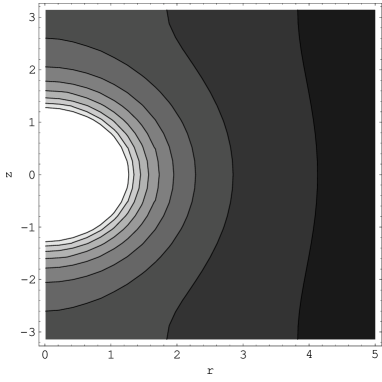
Figure 18: The equipotential lines of the Newtonian potential around a point-like source in 5d drawn in the $(r,z)$ plane. Note the change in their topology from spheres to cylinders.

The $(R,v)$ plane is drawn in figure 19. It is a semi-infinite cylinder with one marked point (denoted by x), which is $(r,z)=(0,L/2)$, where the equipotential surfaces turn from spheres to cylinders and the differential of the transformation from $(r,z)$ to $(R,v)$ vanishes. In these coordinates $R_{0}$, the location of the horizon, is a free parameter that determines the size of the black hole, while the location of the marked point remains fixed at some $R_{1}$. As the black hole grows $R_{0}$ reaches $R_{1}$ and from then on the same equations should generate string solutions rather than BHs (for some appropriate boundary conditions).

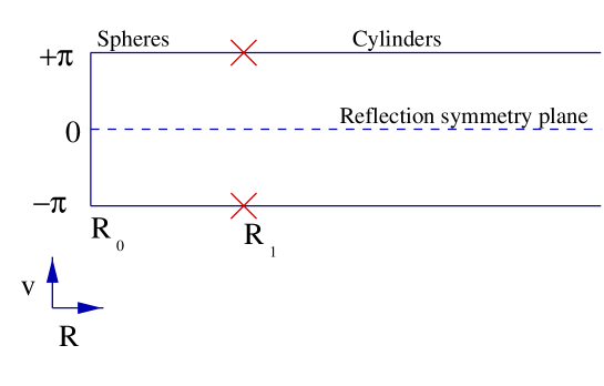
Figure 19: The Harmark-Obers coordinates $R,v$ [67]. $R$ is a function of the Newtonian potential and $v$ is periodic with period $2\pi$. The $x$ marks the point $(R,v)=(R_{1},\pi)$ which is a singular point of the coordinate transformation. For $R<R_{1}$ equal-$R$ surfaces are spheres while for $R<R_{1}$ they are cylinders. The size of the black hole is changed by adjusting $R_{0}$.

In the $(R,v)$ coordinates it turns out that two fields $A,\,K$ suffice (rather than three), according to the following ansatz

$$ds_{d+1}^{2}=f\,dt^{2}+\left({L\over 2\pi}\right)^{2}\left[f^{-1}\,A\,dR^{2}+\frac{A}{K^{d-2}}\,dv^{2}+K\,R^{2}\,d\Omega_{d-2}^{2}\right]$$ (72)

where

$$f=1-\frac{R_{0}^{d-3}}{R^{d-3}}\ .$$ (73)

The justification for this ansatz was demonstrated (in 6d) [69] by showing that for any solution the equations for a change of coordinates to the ansatz (72) are self-consistent. The proof was then generalized in [66] to any dimension. Another way to see that reduction is to write a fully general ansatz by adding a third field $C$, say as the coefficient of $dv^{2}$, and then one finds that the $G_{tt}$ constraint gives an algebraic relation between the three fields [70]. Yet, it is not clear how the reduction of fields could have been anticipated and whether there are other ansatzs with this same property.

A further reduction is possible, expressing $A$ in terms of $K$ and its second derivatives (eq (6.6) of [67]). However, this step makes the equations of order higher than second, and hence unamenable to relaxation (actually even the equations for both $A,K$ were not brought to relaxation form so far).

4.2 Numerical issues

We turn to a brief overview of the numerical implementation issues of our gravito-statics problem. The first simulation of the system was [57] which found the correct prescription for b.c. and constraints and applied it to obtain solutions for non-uniform strings including highly non-uniform ones very close to the merger point. That work benefitted from insights gained from works on the “black hole on a brane” problem such as [71]. A simulated black hole on a brane appeared in [68] while the first simulation for caged BHs appeared simultaneously in [32] (5d) and [33] (6d). However, due to convergence problems large black holes were not possible to obtain. These problems were largely overcome in [34] (5d & 6d) whose figures 16,17 summarize the state of the art.

Implementation. The most important decisions for implementing the numerics are the choice of coordinates, fields and grid. So far the coordinates and fields were chosen in accordance with the conformal gauge (53), with variations intended to extract the singular and asymptotic behavior for smoother numerics. For example, the ansatz used in [57] for 6d strings was

$$ds^{2}={r^{2}\over G_{5}m+r^{2}}\,e^{2\,A}\,dt^{2}+e^{2\,B}(dr^{2}+dz^{2})+e^{2\,C}\,(G_{5}m+r^{2})\,d\Omega^{~{}2}_{3}~{}.$$ (74)

In [32] the implementation proved to be very sensitive to a redefinition of fields, for some unclear reason, the main obstacle being a simple linear redefinition of fields of the form $B^{\prime}=B+C,\,C^{\prime}=B-C$. The more efficient Harmark-Obers coordinates were not implemented so far and it would be interesting to do so.

When choosing a grid one should consider the following factors: the number of nearest neighbors for each point, the density of points and multi-grid issues. Hexagonal lattices are particulary suited for the solution of the Laplace equation in 2d, because one can first use some relaxation method just to distribute the grid points according to a prescribed grid density (to allow for variable grid spacing), and then weights for the discretized Laplacian are uniquely determined from the points’ location. However, for convenience all simulations so far involved square grids and the density of points was sometimes adjusted by using the mapping from grid space to coordinate space. For instance in [32] two grids were used: in the near zone the grid was evenly spaced in $\rho$ and $\cos(\chi)$ (see figure 2 for coordinate definition) while in the asymptotic zone it was evenly spaced in $\log(r),z$. The need for two grids came from the need for different densities of points in the two regions. The price to pay is in the complexities of grid matching. Another grid tool employed in [32] was the “multi-grid” where the problem was relaxed successively on finer and finer grids, in order to accelerate convergence.

Another, less critical choice, is the choice of discretization of the differential operators (such as (50)).

Convergence. Having implemented the numerical scheme, one typically presses “enter” and prays for convergence. To achieve it one is free to use the “convergence speed” parameter $\omega$ (52). Often this does not suffice and we enter the domain of black magic. One difficult problem that arose from an innocent redefinition of the fields was already described.

Another issue involves non-convergence as a result of problems near the exposed $r=0$ axis (so it does not apply to strings). This problem is known to be solved effectively by the following “Wiseman trick” [71]. The field $B$ appears in source terms which are sensitive to errors near the exposed axis and generate instabilities. To cure that one replaces $B$ by a numerically distinct variant, $B2$, which is meant to be more accurate than $B$ near the axis and is gotten by integrating a constraint from the axis outward.

More generally, one expects to have a relation between physical stability of a solution and convergence. However, the method converges nicely for non-uniform strings which are believed to be unstable. The convergence is the result of boundary conditions at the horizon which force the solution to be non-uniform and which perhaps can be described as exerting some “pressure” which stabilizes the string also in the physical sense. It would be nice to understand this issue better.

Tests. The results of the simulations must be tested. The following tests were employed

• Convergence.

• Constraints.

• Integrated first law.

  This law (20) relates $m,\,\tau$ which are measured at infinity with $\beta,\,S$ measured at the horizon. As such it provides a strong overall test of the numerics, and it is satisfying to find that it holds. However, note that the first law does not test the constraints [33, appendix C].

• Comparison with analytic results.

  Some analytic results for small black holes (see subsection 4.4) allow testing of the numerical data. The satisfying agreement is demonstrated in figures 20, 21, 22, 23 taken from [32]. In all figures the size of the BH is measured by $x:=2\,\rho_{h}/L$ where $\rho_{h}$ is the horizon radius in conformal coordinates and this “numerical” definition of $x$, valid in this subsection, should not be confused with a different “analytic” definition of the small parameters $x$ valid in subsection 4.4. Stars, diamonds or triangles represent actual simulation results while the curve represent smooth interpolations which coincide with the theoretical predictions of [28] within the simulation precision.

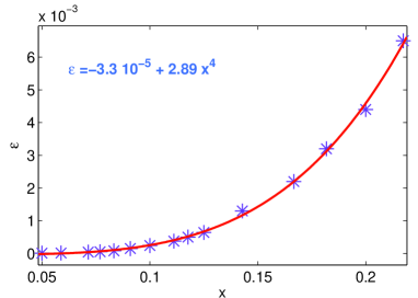
Figure 20: 5d Black hole eccentricity as a function of black hole size. Simulations and perturbative analytic expressions agree. The eccentricity $\epsilon$ is defined in (90). Reproduced from [32].

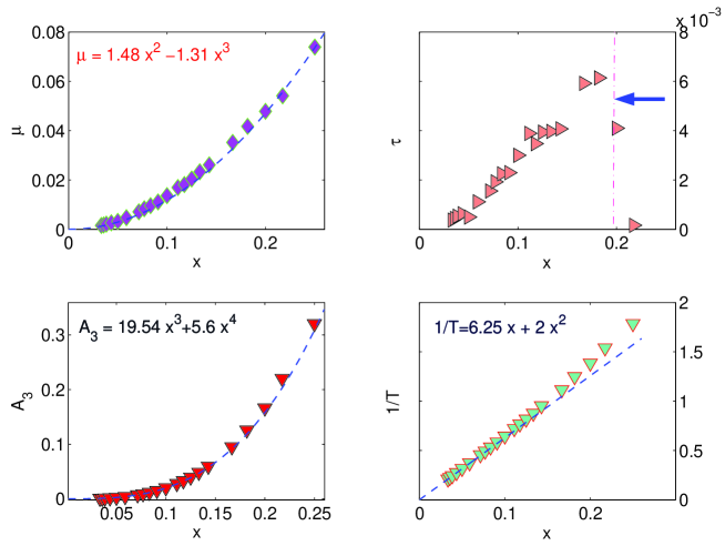
Figure 21: Thermodynamic quantities, $\mu,\,\tau,\,A_{3},\,1/T$ which are the mass, tension, area and inverse temperature, respectively, of a 5d black hole as a function of its size. Simulations and perturbative analytic expressions agree, except for the tension results which are less reliable. Reproduced from [32].

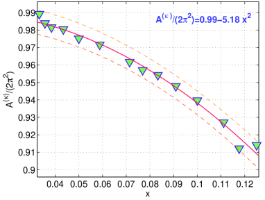
Figure 22: The area in units of the surface gravity, $A^{\kappa}$, as a function of 5d black hole size. This quantity measures a correction to the temperature due to the non-zero potential at the origin from the image BHs. Simulation and perturbative analytic expression agree. Reproduced from [32].

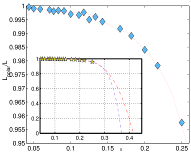
Figure 23: The inter-polar distance (going around the compact dimension), defined in figure 28, as a function of black hole size in 5d. The line denotes a best-fit curve. Its quartic nature is explained in [30], though a theoretical prediction of the prefactor is not presently available. Reproduced from [32].

4.3 Time evolution

As remarked in subsection 2.3, “issues”, the time evolution of the unstable system raises deep questions regarding singularities. Thus there is ample motivation for a dynamical numerical simulation. On the other hand, we expect any such simulation to crash before the singularity is reached. So in order to achieve progress it is probably necessary to have a theoretical local model for the time evolution, which could then be tested and supported by a numerical simulation.

Thus far a single time evolution simulation was performed: [72] simulated the decay of a sub-GL uniform string in 5d. The main features of the evolving spacetime can be read from figure 24. The initial configuration is an unstable string of radius $r_{0}$ on top of which the unstable perturbation grows in time. The region where the horizon moves radially inward (the “waist”) collapses fast, stretching at the same time in the $z$ direction (growing $g_{zz}$) until the minimal (areal) radius reaches about $0.15\,r_{0}$ when the grid stretching is so large that the simulation cannot proceed. In the region where the horizon grows (the “hip”) the metric approaches the metric of a 5d BH with a comparable mass, so that the maximal (areal) radius at the horizon is about $2\,r_{0}$.

Opinions on the interpretation of these results differed. The author of this review interprets them as strong evidence against the formation of a stable non-uniform string end-state. The authors of [72] are much more careful and would only say that the results “are not inconsistent with Gregory and Laflamme’s conjecture that the solution bifurcates into a sequence of black holes … [On the other hand it is] not necessarily inconsistent with [43]… At the same time, a continuation of the observed trend would argue against achieving a stationary solution with a mild dependence on the string dimension”.

Later [73] presented a re-analysis of the metric obtained in [72] which somewhat clarifies the picture. [73] observed that the affine parameter on the horizon grows extremely fast, faster than the exponential of asymptotic time, and suggested that the horizon might pinch off in infinite affine parameter. This possibility was mentioned in [43] but argued against.

In light of the critical dimension $D^{*}=``13.5"$ it would be very interesting to run the simulation again for a range of dimensions, and to test/ confirm that for $D\geq 14$ the unstable string settles down quickly to a slightly non-uniform string.

Figure 24: A time sequence of embedding diagrams for the event horizon of a decaying black string in 5d, from a numerical time evolution. Initially, the string is nearly uniform (top), and by the time the simulation comes to a stop due to grid stretching (bottom), the horizon becomes that of a black hole with a thin pipe connecting the poles (going around the extra dimension). Reproduced with permission from [72].

Method. Let us count the number of degrees of freedom, which is of course larger than in the static case. The domain is the 3d space parameterized by $(r,z,t)$ and the fields are the metric and the scalar which is roughly $g_{\theta\theta}$ or $C$ in (47). The total number of fields is 7. After choosing some gauge in the 3d domain the number of fields reduces to 4 (compared to 3 in the static case). Finally, the “physical” number of degrees of freedom is a total of $0+1=1$ (just like the static case): none for the graviton and +1 for the scalar.

The most general time-dependent metric is

$$ds^{2}=(-\alpha^{2}+\gamma_{AB}\beta^{A}\beta^{B})dt^{2}+2\gamma_{AB}\beta^{A}dx^{B}dt+\gamma_{AB}dx^{A}dx^{B}+\gamma_{\Omega}d\Omega^{2}~{},$$ (75)

where $x^{A}=(r,z)$, and $d\Omega^{2}$ is the 2-spherical line element with coordinates chosen orthogonal to the $t=$ constant congruences (hence there is no shift corresponding to angular directions). All metric components in (75) are defined in the 3d domain. [72] choose the gauge

$$\alpha = \alpha_{St}$$

$$\beta^{z} = 0$$

$$g_{\theta\theta} = r^{2}~{},$$ (76)

where the string metric function is read from the ingoing Eddington-Finkelstein form

$$ds^{2}_{St}=-(1-2M/r)\,d\tilde{t}^{2}+4\,M/r\,dr\,d\tilde{t}+(1+2M/r)\,dr^{2}+dz^{2}+r^{2}\,d\Omega^{2}\,.$$ (77)

They also comment that “In a preliminary version of our code, we also required that $\beta^{r}=\beta_{\rm BS}^{r}$. This, however, caused a coordinate pathology to develop at late times during the evolution of unstable strings—specifically, some regions of the horizons approached a zero coordinate-radius, while maintaining finite proper radius.” Thus the condition on $\beta^{z}$ was replaced by one on $g_{\theta\theta}$.

Another hurdle turned out to be the boundary conditions at infinity. To eliminate cut-off problems spatial infinity was brought to a finite point by replacing $r$ by $r/(r+1)$.

4.4 Analytic perturbation method

While we do not know to write the black hole metric in closed form, metrics for small black holes can be well-approximated everywhere: for $\rho\ll L$ the $D$ dimensional black hole is a good approximation, while for $\rho\gg\rho_{0}$ ($\rho_{0}$ is the Schwarzschild radius) the Newtonian approximation is good. Moreover the two approximations have an arbitrarily large overlap in the small black hole limit. Therefore, one expects that the black hole metric can be systematically expanded in a perturbation series with a small parameter being $x:=\rho_{0}/L$. Such a perturbative method was studied in several papers: the general procedure and first order results were given in [28] (pre-announced in [31]), the full second order in 5d was obtained in [29] and for a general dimension the Post-Newtonian order was performed in [30]. A different, one zone approximation was given in [27].

The objectives here are to

• Provide tests for numerics.

• Extrapolate to the phase transition region.

Method. It is not possible to use here the “usual” perturbation method, the one where a “zeroth order” solution is deformed order by order to follow the deformation of a small parameter of the problem, since here the domain of coordinates changes with $x$, and since we do not have a zeroth order solution. However, one can use the well-known technique of “matched asymptotic expansion”. In [28] this technique was applied by defining two zones: an “asymptotic zone” and a “near horizon zone” (see figure 25), which have a large overlap in the limit $x\to 0$. The metric is solved perturbatively in each zone, with boundary conditions coming from matching with the other zone. The need for matching produces an intricate (and dimension dependent) pattern of crossings between the various orders in the two zones – “the perturbation ladder” – see figure 26. Effectively the gravitational field produced by the images changes the shape of the BH, or its mass multipoles, and that in turn back-reacts and changes the field multipoles. This procedure is much simpler than the usual dynamic matched asymptotic expansion on account of being static, and was therefore given a special name “a dialogue of multipoles” [28].

Figure 25: The metric for small black holes can be obtained through a “dialogue of multipoles” matched asymptotic expansion. The two zones are the asymptotic zone $\rho\gg\rho_{0}$ and the near zone $\rho\ll L$. The smaller the black hole the larger is the overlap region between the two zones.

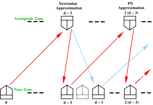
Figure 26: The “perturbation ladder” for the “dialogue of multipoles” matched asymptotic expansion. The upper row depicts the asymptotic zone and the lower row the near zone. Each box denotes a certain order in the perturbation series – in the asymptotic zone one counts orders of $\rho_{0}$ and in the near zone orders of $L^{-1}$. The arrows denote the flow of information between the two zones, in supplying boundary conditions through matching. The figure shows the general pattern for an arbitrary spacetime dimension $D$ ($d$ in the figure is denoted by $D$ in this review). Reproduced from [28].

The zeroth order. In the asymptotic zone the zeroth order metric is flat space with a compact dimension and the origin removed, while in the near zone it is the Schwarzschild black hole, with the periodicity $L$ being far away and invisible.

The Newtonian approximation. The first order analysis in the asymptotic zone is easy – it is just the Newtonian approximation. Here one considers the metric in the weak field limit

$$g_{\mu\nu}=\eta_{\mu\nu}+h_{\mu\nu}\,,$$ (78)

where $\eta_{\mu\nu}$ is the flat space (Minkowski) metric and $h_{\mu\nu}\ll 1$ is a small correction. One defines

$${\bar{h}}_{\mu\nu}:=h_{\mu\nu}-\frac{1}{2}h^{\alpha}_{\alpha}\,\eta_{\mu\nu}\,,$$ (79)

in terms of which the harmonic gauge is chosen

$${\partial}^{\mu}{\bar{h}}_{\mu\nu}=0\,.$$ (80)

The linearized field equations read

$$\frac{1}{2}\,\Box\bar{h}_{\mu\nu}=G_{\mu\nu}=8\pi\,G_{D}\,T_{\mu\nu}\,,$$ (81)

where $\Box$ is the flat space D’alambertian. Solving ${\bar{h}}_{\mu\nu}$ for weak and slowly moving sources where the only non-zero component of $T_{\mu\nu}$ is taken to be $T_{00}$, and inverting (79) through

$$h_{\mu\nu}={\bar{h}}_{\mu\nu}-\frac{1}{D-2}{\bar{h}}^{\alpha}_{\alpha}\,\eta_{\mu\nu}\,,$$ (82)

we find

$$h_{tt} = \Phi_{N},$$

$$h_{ij} = \frac{1}{D-3}\,\Phi_{N}\,\delta_{ij},$$ (83)

where the Latin indices stand for the spatial components and $\Phi_{N}$ is a the Newtonian potential (69). In the $D=5$ case there is a useful way to perform the summation in the definition of $\Phi_{N}$ (69), yielding

$$\Phi_{N}=\rho_{0}^{2}\,{\pi\over L\,r}\,\frac{\sinh\left(\frac{2\,\pi\,r}{L}\right)}{\cosh\left(\frac{2\,\pi\,r}{L}\right)-\cos\left(\frac{2\,\pi\,z}{L}\right)}\,.$$ (84)

Linear perturbations around Schwarzschild . The first correction to the near zone requires more work than the Newtonian approximation in the asymptotic zone – it is a generalization to higher $D$ of the well-known paper by Regge and Wheeler [74]. The metric is given in terms of a single function $E=E(\rho,\chi)$ which determines the metric. After separation of variables, $E_{l}(\rho)$ satisfies a “master equation”

$$\frac{D^{2}\,E}{dX^{2}}+\left(\frac{2}{X}+\frac{1}{X-1}-\frac{1}{X-w}\right)\,\frac{d\,E}{dX}-p\,(1+p)\frac{X+(D-4)\,w}{X\,(X-1)\,(X-w)}\,E=0$$ (85)

where $l$ is the angular momentum and

$$X := (\rho/\rho_{0})^{D-3}$$

$$w_{l,D} := -\frac{D-2}{(l-1)\,(l+D-2)}$$

$$p_{l,D} := \frac{l}{D-3}~{}.$$ (86)

There are four regular singularities in the complex plane including $\infty$, so it is a “Heun equation”, by definition. The singularities are at $0,\rho_{0},\infty$ and at $w$, but the latter can be eliminated by a field re-definition (re-defining $E$) and in that sense is “non-physical”. Since there are 3 remaining singularities the solutions can be expressed in terms of hyper-geometric functions. These results were first obtained in [76] and then in [28] each using somewhat different methods.

Regulation of divergences at Post-Newtonian order. At the next, Post-Newtonian order divergences were identified and regulated in [30]. The divergences originate from integration over the non-compact overlap region (which is the neighborhood of the origin for the asymptotic zone). The regularization can be defined through a “cut-off and match” method where one places a cut-off on the integral, matches with the other zone, and then sends the cut-off away to remain with a finite solution. This is equivalent to a regularization known as Hadamard’s partie finie, and it is closely related to the concept of “subtracting the self-energy”. This regularization allowed to obtain the thermodynamic quantities at Post-Newtonian order.

In [27] an alternative method was given employing a single patch, and using the efficiency of Harmark-Obers coordinates [67]. There a “first order” approximation is given, and I expect that the method could be developed to a full perturbation series by successively improving a suitably chosen initial guess. It has the advantage of using only a single zone, and doing away with matching. However, the method depends on the choice of initial guess, and unlike the previous method, the differential operator to be inverted would probably change at each order.

Results. In 5d the second order metric was obtained in [29] from which the following thermodynamics were deduced

$$S = {\pi^{2}\,L^{3}\over 2\,G_{5}}\,\tilde{\epsilon}^{3/2}\,\left(1+{\pi^{2}\,\tilde{\epsilon}\over 8}+{\pi^{2}\,\tilde{\epsilon}^{2}\over 384}\right)$$

$$T = {1\over 2\pi\,\mu}\,\tilde{\epsilon}^{3/2}\,\left(1-{5\pi^{2}\tilde{\epsilon}\over 24}+{43\pi^{4}\,\tilde{\epsilon}^{2}\over 1152}\right)$$

$$\tau\,L/M = {\pi^{2}\tilde{\epsilon}\over 6}-{\pi^{4}\,\tilde{\epsilon}^{2}\over 36}~{},$$ (87)

where the small parameter is defined through $\tilde{\epsilon}=8\,G_{5}\,M/(3\pi\,L^{2})=\rho_{0}^{2}/L^{2}$.

For arbitrary $D$ the best available determinations of the thermodynamics quantities [28, 27, 30] are

$$S = {\Omega_{D-3}\over 4}\,\rho_{0}^{~{}D-2}\left[1+{D-2\over D-3}\,\delta\right]$$

$$T = {D-3\over 4\pi\,\rho_{0}}\left[1-(D-2)\,\delta\right]$$

$$\tau\,L/M = {D-3\over 2}\,\delta$$

$$M = {(D-2)\,\Omega_{D-2}\over 16\pi\,G_{N}}\,\rho_{0}^{~{}D-3}\left[1+{1\over 2}\,\delta\right]~{},$$ (88)

where

$$\delta:=\zeta(D-3)\,\left({\rho_{0}\over L}\right)^{D-3}~{},$$ (89)

and $\zeta(s):=\sum_{n=1}^{\infty}1/n^{s}$ is Riemann’s zeta function, which appears here due to the sum over black hole images. We note that the black hole tension (88) vanishes to lowest order, namely $O(M)$ and the leading order result can be explained by the Newtonian potential between the black hole and its images [30].

When one considers results beyond the leading order, such as some of the results above, their “scheme dependence” should be borne in mind. “Scheme dependence” is used here to mean the freedom to re-parameterize $\rho_{0}$ and through it the branch of small black hole solutions: while to leading order all definitions of $\rho_{0}$ coincide (up to a multiplicative constant), there is no unique or natural definition for the subleading corrections, and therefore results should be accompanied by a specification of the scheme in which they were obtained. In particular, the definition used in [30] is specified in [28], subsection 3.3.2.

Some nice geometric quantities can be measured as well. The leading deviation from spherical shape is such that the BH becomes elongated along the $z$ axis, namely prolate – see figure 27. Its eccentricity can be measured by

$$\epsilon:={A_{\perp}\over A_{\parallel}}-1={(D-3)^{4}\,\Gamma^{2}(2+{2\over D-3})\,\zeta(D-1)\over 8(D-2)\,\Gamma({4\over D-3})}\left({\rho_{0}\over L}\right)^{D-1}~{}.$$ (90)

This result actually comes from beyond first order. The inter-polar distance (going around the compact dimension, see figure 28) is given by

$$L_{\mbox{poles}} = L-2^{D-5\over D-3}\,\rho_{0}\,I_{D}+\dots$$

$$I_{D} = 4^{1\over D-3}\,\sqrt{\pi}{\Gamma({D-4\over D-3})\over\Gamma({1\over 2}-{1\over D-3})}~{}.$$ (91)

where the ellipsis is order $o\left((\rho_{0}/L)^{D-2}\right)\cdot L$. Since $I_{5}=0$ in 5d the black hole makes room for itself, exactly compensating its size, and for that reason it was called “the black hole Archimedes effect” [32]. More precisely, in 5d $L_{\mbox{poles}}/L=o\left((\rho_{0}/L)^{3}\right)$, and numerical results indicate that indeed the next order is non-zero: $L_{\mbox{poles}}/L=O\left((\rho_{0}/L)^{4}\right)$. For higher $D$, $~{}0<I_{D}<1$, the effect is milder, and in addition, the order of the ellipsis depends on a choice of scheme defined by eq. (B.15) of [30].

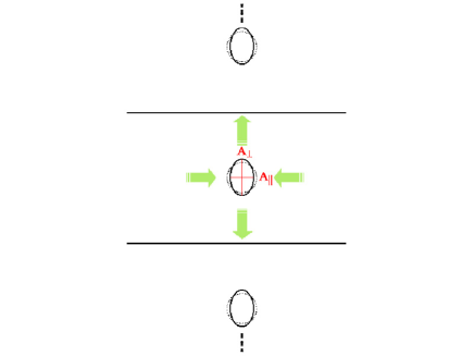
Figure 27: The first non-spherical deformation of the horizon is a quadruple moment, making the black hole prolate, namely elongated along the $z$ axis. In order to measure the eccentricity we define $A_{\parallel}$ the area of the equator sphere and $A_{\perp}$ the area of a “polar” sphere.

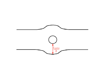
Figure 28: The inter-polar distance is defined to be the proper distance between the poles, going around the compact dimension. The figure depicts the tendency of mass to “make room for itself”, an phenomenon termed “the black hole Archimedes effect” in [32].

Impact on objectives. The ability to produce results for small black holes from two quite different methods, perturbation theory and numerical analysis, allowed for a healthy feedback between the two, testing and perfecting each one of them – see subsection 4.2 and especially figures 20, 21, 22, 23. While the perturbative method does not apply directly to the phase transition region, it provided important tests for the numerics which are capable to study that region.

Implications for the phase diagram. Even though the phase transition region is outside the domain of validity of the perturbative method, the results above can be extrapolated to provide evidence [30] for the critical dimension separating first and second order behavior, as we now proceed to explain (of course chronologically $D^{*}$ was discovered first by [42]). By extrapolating the result for the tension of the small black hole (88) one obtains an extrapolated straight line in the phase diagram whose intersection with the $b=0$ axis, called $\mu_{X}$, should be compared with $\mu_{GL}$ the critical Gregory-Laflamme mass. While for small $D$ numerically one finds that $\mu_{X}>\mu_{GL}$, for large $D$ examination of the asymptotic expansions show that $\mu_{X}\ll\mu_{GL}$, which means that for large $D$ the black hole phase is not available yet at the onset of the GL instability and therefore the string must decay to a different phase, which is evidence for the smooth second order decay into the stable non-uniform string.

5 Related work

Here we mention some related work.

Relation with gauge theory & charged black holes. The gravitational phase transition is closely related to a gauge theory phase transition, the so-called “Gross-Witten” transition [77] where the eigenvalues of some unitary matrix (originally a Wilson line over a plaquette, in a later application [78], a Wilson line around a compact dimension) change from a clumped distribution to a uniform one as the temperature is raised (see figure 29). This correspondence was first noted by Susskind (1997) [79] on a somewhat qualitative level and was fully analyzed quantitatively by Aharony-Marsano-Minwalla-Wiseman in [78]. The correspondence with gauge theory enriches the system by adding another parameter to the problem – the coupling.

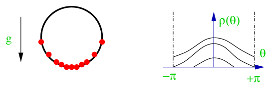
Figure 29: In the Gross-Witten phase transition [77] the dynamics of the eigenvalues of a unitary matrix in gauge theory is mapped to a system of particles in a horizontal loop in the field of gravity. In large $N$ (the number of particles) the particle density becomes a continuous function $\rho(\theta)$. The phase transition is between localized to non-uniform and then to uniform distributions. Susskind (1997) identified this phenomenon as the gauge theory dual of the black-hole black-string transition.

In [80] the authors showed that the phase diagram of black holes/strings directly maps onto the phase diagram of near-extremal black branes, and hence via holography onto the phase diagram of the dual non-gravitational theories (Super-Yang-Mills and “Little String Theory”). More specifically, they present the phases of the non-gravitational theories and analytical results for the thermodynamics of the localized phase and the new non-uniform phase (connected to the “image” of the GL point). In fact part of the early motivation of these authors for studying black holes in Kaluza-Klein backgrounds (see [67]) has been precisely that, namely to relate it to gauge theories. See also the brief review [81].

In [82] the GL analysis was generalized to “point-like” charged strings, and the instability was found to persist for all charges, and moreover $k_{GL}$ diverges as extremality is approached.

For ideas about the relation of this phase transition to the Hagedorn phase transition in string theory see [83] and references therein.

Bubbles. Taking the metric of the black string (3) and performing a double analytic continuation in $z,t$ (namely $t^{\prime}=iz,\,z^{\prime}=it$) one gets an unstable metric called the “bubble”. In the Euclidean setting the analog would be to exchange $\beta\leftrightarrow L$ thereby inverting $\mu_{\beta}$, which is not that interesting. From the Lorentzian perspective this is another phase that could be put on the same phase diagram. It has the special property $\tau\,L=(D-3)M$. Thus the bubble exactly saturates the Strong Energy Condition upper bound on tension (see subsection 3.1), which motivated [51] to study this phase as well as combinations of several bubbles and BHs. So far bubble phases were not seen to connect with the phases discussed in this review, so it is conceivable that the two issues are decoupled. See also the brief review [81].

Braneworld black holes. The topic of black holes on braneworlds is closely related to the subject of this review. There the dimensionless parameter is the ratio of the black hole size and the size of AdS. A comprehensive bibliography is beyond the scope of this paper, but we shall only mention braneworld work [71, 84, 68, 85] which was followed by work on compact dimensions.

6 Summary and Open questions

Why review. We start with a description of some of the major recent developments in the field from a personal perspective, leading to the decision that the field is ripe for this review to be written.

The Gregory-Laflamme instability and the whole black-hole black-string transition have been attracting constant attention in the String Theory community as well as in General Relativity since its discovery (1993). In may 2001 the interest rose further due to the provoking ideas in [43]. A year later I suggested in [44] a qualitative form for the phase diagram which proposed the merger of the black hole and black string phases, and rested on Morse theory and a topology change analysis. Even today that paper includes most of what I know about the system, but back then many felt that the evidence was not convincing enough, and the paper was even refused for publication by two leading journals. The non-trivial nature of these predictions is best illustrated by the various other possibilities that were considered in the literature, see for example the six scenarios in [66], section 6.

Now, after more than two years and more than 30 papers, we have a much more detailed knowledge of the phase diagram, culminating in the numeric results of [34] which combine new numerical data for black holes with older data for non-uniform strings into a full phase diagram (figure 16). This full, actual-data phase diagram exhibits the merger of the phases, vindicating [44], concluding most of the uncertainty around [43, 44] as we discuss further below, and providing a natural point in time to write a review.

Below we summarize the results and open questions. The results include two big surprises: critical dimensions and topology change, but we remind the reader that while there was much progress in understanding the static phase diagram, there was practically no progress towards the deeper issues regarding time evolution and singularities.

6.1 Results

• Confirmation of emerging phase diagram.

  The current understanding of the qualitative features of the phase diagram is summarized in figure 15, where the $D\leq 13$ case originates in [44]. We note that all diagrams include a merger point.

  For $D\leq 13$ the end-point of decay is seen to be a black hole, and not a stable black string which was predicted in [43]. The evidence for that includes a numerical determination of practically the whole branch of the non-uniform string which emerges from the GL point and was found to have higher mass than the critical string and thus cannot serve as an end-point for decay [57]; the continued collapse of a time evolution simulation [72], coming to a stop due to grid stretching, rather than the predicted stabilization; theoretical difficulties in proposing a phase diagram which includes the predicted phase and satisfy the Morse theory constraint [44]; and finally the fact that such a phase was not found neither analytically (see the attempt of [86]) nor numerically.

  For $D\geq 14$ the end-point of (smooth) decay does turn out to be a stable non-uniform string (as a result of [42]), thus partially vindicating [43]. However, I claim that in a deeper sense, this case does not validate the arguments of [43]. First, the arguments were independent of dimension, and second, even for $D\geq 14$, horizon pinching, which [43] finds to be forbidden, must happen after the non-uniform string evaporates enough.

  Thus while the claim of [43] stimulated much of the research reported here, and while there is no doubt regarding the calculations presented there, we find strong (actually, overwhelming in my opinion) evidence against it. One should therefore reconcile the derivation in [43] with the results presented above. However, it is clear that if something went wrong in the arguments of [43] it is rather deep and there are lessons to be learned from it. Following the analysis of the numerical time evolution in [73] it seems that while indeed pinching does not occur in finite horizon affine parameter, consistent with the findings of [43], it could well happen with infinite horizon affine parameter and finite asymptotic time (see also [87]). This possibility was indeed discussed in [43], and finally rejected, but with less certainty. In [88] this point of view seems to have been accepted: “It was conjectured by Kol [14] that the nonuniform black strings should meet the squashed black holes at a point corresponding to a static solution with a singular horizon, and this appears to be the case [15]. …the black string horizon might pinch off in infinite affine parameter… … [the] suggestion … that the black string will break up into spherical black holes might still be correct.” Altogether, it looks like a reasonable consensus arises where the central calculation of [43] holds and only the arguments against pinching in infinite time had some loop-hole, which invalidates, however, their bottom-line conclusion regarding the end-point of the decay into stable non-uniform strings.

  Another possibility for a flaw in the assumptions of [43] should be mentioned, namely the reliance on the increasing area of the event horizon. Even though the authors were careful to use a version of the theorem valid even if there is a singularity on the horizon, it is still quite possible that in the present context the whole notion of the event horizon is ill-defined and/or that the singularity completely leaves the horizon. The problem with the definition of the event horizon is that if a singular shock wave emerges from a naked singularity and reaches null infinity, then we do not have the asymptotically Minkowski null infinity which is normally used in the definition. Clearly, this issue, like others involving the time evolution, is not well understood yet.

• Critical dimensions.

  The stability of cones, which have a role in the local model for merger, exhibits a critical dimension $D^{*}_{\mbox{merger}}=10$ [44], see subsection 3.4. At a different point in the phase diagram, the GL instability changes from explosive (first order) to smooth (second order) for $D>D^{*}_{GL}=13.5$, as was shown by Sorkin [42]. For the canonical ensemble this happens at $D>D^{*}_{GL,c}=12.5$ [58].

  These critical dimensions are fascinating, but it is not known whether they have a deeper, wider meaning. The critical dimension of the BKL theory of the approach to a space-like singularity, $D^{*}=10$, is closely related. On the one hand one cannot help wondering whether there could be a connection with the critical dimension for super-strings, 10d, but on the other hand the derivations and issues involved differ widely, for example, in the phase transition no supersymmetry is involved while it is central for the super-string.

• The “merger” topology change [44].

  The spaces of metrics for two different topologies, the Euclidean black string and the black hole (in $D\geq 5$) are glued together (subsection 3.4) and a line of Ricci flat solutions connects them, see subsection 3.4 (in finite distance, see appendix B).

Additional results include

• The use of Morse theory in GR [44], described in subsection 3.3.

• The role of tension and the first law for this system [46, 31], subsection 3.1.

• Formulating Gravito-statics by relaxation (in 2d) [57], subsection 4.1.

• Numerical solutions: strings [57] and black holes [32, 33, 34], subsection 4.2, and a dynamic time-evolution [72], subsection 4.3.

• Developing an analytic perturbation method for small caged black holes – “a dialogue of multipoles” [28, 29]. See [27] for a different analytic method. Described in subsection 4.4.

6.2 Open questions

• The deepest questions remain: are there a naked singularity and perhaps, a singular shock wave in the time evolution? – see the discussion in subsection 2.3. This problem could benefit from both a theoretical approach and from numerical analysis.

• Obtain solutions with discrete self-similarity (DSS) which were conjectured in [63] to describe the merger solution locally near the pinch point (in progress).

• Gubser and Mitra [36] conjectured already in 2000 a connection between perturbative and thermodynamic instabilities of strings which is closely related to the issues of this review. It found confirmation in several cases, some recent ones being [89, 90, 91] (in the last case what appeared to be counter-examples became consistent with the conjecture after appropriately generalizing it to allow for scalar fields). It would be interesting to settle this conjecture.

• Formulate gravito-statics in more than 2d.

• Numerically trace the phase diagram also for additional dimensions in the ranges $10<D\leq 13$ and $D\geq 14$.

• Run a time evolution for $D\geq 14$ to observe the second order transition.

Two items present when the first version of this review appeared in the archives, are by now mostly resolved

• Determine the critical dimension for torus compactifications.

  – torus compactifications do not reduce the critical dimension [18].

• Stability analysis in the micro-canonical ensemble. In the canonical ensemble the Morse analysis, which identifies the thermodynamic potential $F$ with a Morse function, allows us to read the stability of phases off the phase diagram. It is plausible that a generalization to other ensembles exists. For instance, that would allow to settle the conjectured (micro-canonical) instability of the non-uniform string (for $D<14$).

  – Poincaré’s method (see [60] for a review) teaches us that indeed the stability in the micro-canonical ensemble can be determined from the form of the phase diagram just like in the canonical ensemble, since stability changes can occur only at turning points or at vertices where several phases meet.

The ring. We list some questions regarding the physics of the sister system of rotating rings, even though they are not part of the main subject of this review.

• Obtain the full phase diagram: stability of phases, order of transition, critical points.

• Solutions in $D>5$?

Acknowledgements

It is a pleasure to thank Toby Wiseman, Niels Obers and especially an anonymous referee for reading the paper and making comments on it, the authors of [34, 42, 72, 17, 28] for permission to reproduce their figures and especially for adapting them, in some cases, for this review; my collaborators Dan Gorbonos, Tsvi Piran, Evgeny Sorkin and Toby Wiseman with whom I worked on this topic; Hideaki Kudoh, Luis Lehner and Niels Obers for discussions and correspondence; John Bahcall, Gary Gibbons, Gary Horowitz, and Lenny Susskind for discussions and inspiration; Roberto Emparan, Steve Gubser, Akihiro Ishibashi, Igor Klebanov, Hermann Nicolai, Mukund Rangamani, Edward Witten for some specific discussions; and finally Shmu’el Elitzur, Amit Giveon, and Eliezer Rabinovici my group partners in Jerusalem for their assistance during these two first years of mine here. I also wish to thank the following institutions for their hospitality during the course of the work reviewed here: Max-Planck Institute at Golm, Humboldt University Berlin, Cambridge University, Amsterdam University, the Perimeter Institute, MIT and Harvard University.

BK is supported in part by The Israel Science Foundation (grant no 228/02) and by the Binational Science Foundation BSF-2002160.

Appendix A Formulae for action manipulation

Here we collect some formulae which are useful for manipulation of actions.

The Ricci scalar in the presence of a general fibration

$$ds^{2} = ds^{2}_{X}+\sum_{i}\,e^{2\,F_{i}}\,ds^{2}_{Yi}\Rightarrow$$

$$R = R_{X}+\sum_{i}\,[e^{-2\,F_{i}}\,R_{Yi}-2\,d_{i}\,\widetilde{\triangle}(F_{i})-d_{i}({\partial}F_{i})^{2}]-\sum_{i,j}\,d_{i}\,d_{j}\,({\partial}F_{i}\cdot{\partial}F_{j})$$ (92)

where the fibration fields depend only on the $x$ coordinates $F_{i}=F_{i}(x)$, $R_{X},~{}R_{Yi}$ are the Ricci scalars of the spaces $X,\,Y_{i}$, $d_{i}$ are the dimensions $\mbox{dim}(Y_{i})$, and the Laplacian ($\widetilde{\triangle}$) and grad-squared (${\partial}\cdot{\partial}$) are evaluated in the X space.

The Ricci scalar of a conformally transformed metric (see for example [92])

$$\widetilde{ds}^{2} = e^{2\,w}\,ds^{2}\Rightarrow$$

$$\widetilde{R} = e^{-2\,w}\,[R-2\,(\hat{d}-1)\,\triangle w-(\hat{d}-1)(\hat{d}-2)\,({\partial}w)^{2}]$$ (93)

where $\hat{d}$ is the dimension of the space and the Laplacian and grad-squared are evaluated in the non-tilded metric.

Appendix B Topology change is a finite distance away

Scaling down a smoothed cone gives a family of metrics which approaches the singular cone, as discussed is subsection 3.4 (see figure 14). In this appendix we wish to show that the singular cone is at a finite distance in moduli space, just like the conifold.

Let us denote a smooth cone metric with some specific length scale (of the smoothed tip) by

$$\widetilde{ds}^{2}=d{\tilde{\rho}}^{2}+e^{2\,a({\tilde{\rho}})}\,d\Omega^{2}_{{\bf S}^{m}}+e^{2\,b({\tilde{\rho}})}\,d\Omega^{2}_{{\bf S}^{n}}~{}.$$ (94)

The family of rescaled cone metrics is defined by

$$ds^{2}=e^{-2\sigma}\,\widetilde{ds}^{2}~{},$$ (95)

and we wish to compute the distance in moduli space from $\sigma=0$ to $\sigma=\infty$ ($\sigma=\infty$ is the non-smooth cone).

The metric on moduli space can be found by adding an auxiliary coordinate $t$, making $\sigma$ $t$-dependent, $\sigma=\sigma(t)$, and evaluating its kinetic term. Since one wants to hold the asymptotic form of the cone fixed it is useful to introduce $\rho=e^{-\sigma}\,{\tilde{\rho}}$. Then the rescaled cone metric is $ds^{2}=d\rho^{2}+e^{2\,(a(\rho e^{\sigma})-\sigma)}\,d\Omega_{m}+e^{2\,(b(\rho e^{\sigma})-\sigma)}\,d\Omega_{n}$ , where $d\Omega_{m}=d\Omega^{2}_{{\bf S}^{m}}$. Adding $t$-dependence and substituting back to ${\tilde{\rho}}$ we get

$$ds^{2}=dt^{2}+e^{-2\sigma}\,\left[(d{\tilde{\rho}}-\dot{\sigma}\,{\tilde{\rho}}\,dt)^{2}+e^{2\,a}\,d\Omega_{m}+e^{2\,b}\,d\Omega_{n}\right]$$ (96)

Using (92) the Ricci scalar is

$$R = -m(m+1)\,({\partial}(a-\sigma))^{2}-2\,m\,\triangle(a-\sigma)$$ (97)

$$-n(n+1)\,({\partial}(b-\sigma))^{2}-2\,n\,\triangle(b-\sigma)$$

$$-2\,m\,n\,{\partial}(a-\sigma)\,{\partial}(b-\sigma)~{},$$

where the differential operators are in the $({\tilde{\rho}},t)$ plane. All terms which vanish when $\dot{\sigma}=0$ must cancel since the resolved cone is Ricci-flat, and one finds

$$R = -2\left[(m\,a^{\prime}+n\,b^{\prime}){\tilde{\rho}}-(D-1)\right]\,\ddot{\sigma}$$

$$+ \dot{\sigma}^{2}\left[-{\tilde{\rho}}^{2}(m(m-1)\,e^{-2\,a}+n(n-1)\,e^{-2\,b})+2\,{\tilde{\rho}}\,(D-1)(m\,a^{\prime}+n\,b^{\prime})-D(D-1)\right]$$

A useful test for this expression is that it must vanish when substituting the singular cone metric rather than the resolved cone.

The resulting bulk action after multiplying by $\sqrt{g}=e^{m\,a+n\,b-D\,\sigma}$ and eliminating the second derivatives using integration by parts is

$$S = \int dt\,\dot{\sigma}^{2}\,e^{-D\,\sigma}\int d{\tilde{\rho}}\,e^{m\,a+n\,b}\,$$

$$\cdot \left[-{\tilde{\rho}}^{2}(m(m-1)\,e^{-2\,a}+n(n-1)\,e^{-2\,b})-2\,{\tilde{\rho}}(m\,a^{\prime}+n\,b^{\prime})+D(D-1)\right]$$

This action should be regularized by comparison with the singular cone. This can be done by introducing a large-distance cut-off $\rho=\Lambda$ and therefore ${\tilde{\rho}}_{\Lambda}=\Lambda\,e^{\sigma}$ and subtracting for the cone. We are interested in large $\sigma$ and hence ${\tilde{\rho}}_{\Lambda}\to\infty$. In this limit the integral seems to be dominated by the large ${\tilde{\rho}}$ behavior of the integrand: the large ${\tilde{\rho}}$ behavior of $a,\,b$ compared to the singular cone is given by the linearized perturbations (44)

$$\delta a,\,\delta b\sim\rho^{s},~{}~{}\mbox{Re}(s)=-(D-2)/2$$ (100)

The large ${\tilde{\rho}}_{\Lambda}$ behavior of the kinetic term in (B) is

$$e^{-D\,\sigma}\,\int^{\Lambda\,e^{\sigma}}d{\tilde{\rho}}\,{\tilde{\rho}}^{D-1}\,{\tilde{\rho}}^{-(D-2)}\sim e^{-D\,\sigma}(\Lambda^{2}\,e^{2\,\sigma})~{}~{}.$$ (101)

Hence the metric on moduli space in the large $\sigma$ limit is

$$ds^{2}_{\cal M}=e^{-(D-2)\,\sigma}\,d\sigma^{2}$$ (102)

and the distance is finite

$$\int^{+\infty}\exp(-{D-2\over 2}\,\sigma)\,d\sigma<\infty$$ (103)

for $D>2$, namely always, since we were only interested in $D\geq 5$.

References

- [1] T. Damour, M. Henneaux, and H. Nicolai, Cosmological billiards, Class. Quant. Grav. 20 (2003) R145–R200, [hep-th/0212256].
- [2] P. O. Mazur, Black hole uniqueness theorems, hep-th/0101012. p.10-11.
- [3] R. Emparan, Rotating circular strings, and infinite non-uniqueness of black rings, JHEP 03 (2004) 064, [hep-th/0402149].
- [4] I. Bena and N. P. Warner, One ring to rule them all … and in the darkness bind them?, hep-th/0408106.
- [5] H. Elvang, R. Emparan, D. Mateos, and H. S. Reall, Supersymmetric black rings and three-charge supertubes, Phys. Rev. D71 (2005) 024033, [hep-th/0408120].
- [6] B. Kol, Speculative generalization of black hole uniqueness to higher dimensions, hep-th/0208056.
- [7] C. Helfgott, Y. Oz, and Y. Yanay, On the topology of black hole event horizons in higher dimensions, hep-th/0509013.
- [8] G. J. Galloway and R. Schoen, A generalization of Hawking’s black hole topology theorem to higher dimensions, gr-qc/0509107.
- [9] S. W. Hawking and J. M. Stewart, Naked and thunderbolt singularities in black hole evaporation, Nucl. Phys. B400 (1993) 393–415, [hep-th/9207105].
- [10] R. C. Myers and M. J. Perry, Black holes in higher dimensional space-times, Ann. Phys. 172 (1986) 304.
- [11] R. Emparan and H. S. Reall, A rotating black ring in five dimensions, Phys. Rev. Lett. 88 (2002) 101101, [hep-th/0110260].
- [12] H. Elvang, R. Emparan, D. Mateos, and H. S. Reall, A supersymmetric black ring, Phys. Rev. Lett. 93 (2004) 211302, [hep-th/0407065].
- [13] G. Arcioni and E. Lozano-Tellechea, Stability and thermodynamics of black rings, hep-th/0502121.
- [14] J. P. Gauntlett and J. B. Gutowski, Concentric black rings, Phys. Rev. D71 (2005) 025013, [hep-th/0408010].
- [15] J. P. Gauntlett and J. B. Gutowski, General concentric black rings, Phys. Rev. D71 (2005) 045002, [hep-th/0408122].
- [16] H. Elvang, R. Emparan, and P. Figueras, Non-supersymmetric black rings as thermally excited supertubes, JHEP 02 (2005) 031, [hep-th/0412130].
- [17] B. Kol and E. Sorkin, On black-brane instability in an arbitrary dimension, Class. Quant. Grav. 21 (2004) 4793–4804, [gr-qc/0407058].
- [18] B. Kol and E. Sorkin. to appear.
- [19] R. C. Myers, Higher dimensional black holes in compactified space- times, Phys. Rev. D35 (1987) 455.
- [20] D. Korotkin and H. Nicolai, A periodic analog of the Schwarzschild solution, gr-qc/9403029.
- [21] A. V. Frolov and V. P. Frolov, Black holes in a compactified spacetime, Phys. Rev. D67 (2003) 124025, [hep-th/0302085].
- [22] N. Itzhaki, J. M. Maldacena, J. Sonnenschein, and S. Yankielowicz, Supergravity and the large n limit of theories with sixteen supercharges, Phys. Rev. D58 (1998) 046004, [hep-th/9802042].
- [23] S. A. Abel, J. L. F. Barbon, I. I. Kogan, and E. Rabinovici, String thermodynamics in D-brane backgrounds, JHEP 04 (1999) 015, [hep-th/9902058].
- [24] A. Chamblin, S. W. Hawking, and H. S. Reall, Brane-world black holes, Phys. Rev. D61 (2000) 065007, [hep-th/9909205].
- [25] R. Emparan, G. T. Horowitz, and R. C. Myers, Exact description of black holes on branes, JHEP 01 (2000) 007, [hep-th/9911043].
- [26] F. R. Tangherlini, Schwarzschild field in dimensions and the dimensionality of space problem, Nuovo Cim. 27 (1963) 636.
- [27] T. Harmark, Small black holes on cylinders, Phys. Rev. D69 (2004) 104015, [hep-th/0310259].
- [28] D. Gorbonos and B. Kol, A dialogue of multipoles: Matched asymptotic expansion for caged black holes, JHEP 06 (2004) 053, [hep-th/0406002].
- [29] D. Karasik, C. Sahabandu, P. Suranyi, and L. C. R. Wijewardhana, Analytic approximation to 5 dimensional black holes with one compact dimension, Phys. Rev. D71 (2005) 024024, [hep-th/0410078].
- [30] D. Gorbonos and B. Kol, Matched asymptotic expansion for caged black holes: Regularization of the post-Newtonian order, Class. Quant. Grav. 22 (2005) 3935–3959, [hep-th/0505009].
- [31] B. Kol, E. Sorkin, and T. Piran, Caged black holes: Black holes in compactified spacetimes. I: Theory, Phys. Rev. D69 (2004) 064031, [hep-th/0309190].
- [32] E. Sorkin, B. Kol, and T. Piran, Caged black holes: Black holes in compactified spacetimes. II: 5d numerical implementation, Phys. Rev. D69 (2004) 064032, [hep-th/0310096].
- [33] H. Kudoh and T. Wiseman, Properties of Kaluza-Klein black holes, Prog. Theor. Phys. 111 (2004) 475–507, [hep-th/0310104].
- [34] H. Kudoh and T. Wiseman, Connecting black holes and black strings, Phys. Rev. Lett. 94 (2005) 161102, [hep-th/0409111].
- [35] R. Gregory and R. Laflamme, Black strings and p-branes are unstable, Phys. Rev. Lett. 70 (1993) 2837–2840, [hep-th/9301052].
- [36] S. S. Gubser and I. Mitra, Instability of charged black holes in anti-de Sitter space, hep-th/0009126.
- [37] S. S. Gubser and I. Mitra, The evolution of unstable black holes in anti-de Sitter space, JHEP 08 (2001) 018, [hep-th/0011127].
- [38] H. S. Reall, Classical and thermodynamic stability of black branes, Phys. Rev. D64 (2001) 044005, [hep-th/0104071].
- [39] R. Gregory and R. Laflamme, The instability of charged black strings and p-branes, Nucl. Phys. B428 (1994) 399–434, [hep-th/9404071].
- [40] D. J. Gross, M. J. Perry, and L. G. Yaffe, Instability of flat space at finite temperature, Phys. Rev. D25 (1982) 330–355.
- [41] R. Gregory and R. Laflamme, Hypercylindrical black holes, Phys. Rev. D37 (1988) 305.
- [42] E. Sorkin, A critical dimension in the black-string phase transition, Phys. Rev. Lett. 93 (2004) 031601, [hep-th/0402216].
- [43] G. T. Horowitz and K. Maeda, Fate of the black string instability, Phys. Rev. Lett. 87 (2001) 131301, [hep-th/0105111].
- [44] B. Kol, Topology change in general relativity and the black-hole black-string transition, hep-th/0206220.
- [45] B. Kol, Explosive black hole fission and fusion in large extra dimensions, hep-ph/0207037.
- [46] T. Harmark and N. A. Obers, New phase diagram for black holes and strings on cylinders, Class. Quant. Grav. 21 (2004) 1709, [hep-th/0309116].
- [47] J. H. Traschen and D. Fox, Tension perturbations of black brane spacetimes, Class. Quant. Grav. 21 (2004) 289–306, [gr-qc/0103106].
- [48] P. K. Townsend and M. Zamaklar, The first law of black brane mechanics, Class. Quant. Grav. 18 (2001) 5269–5286, [hep-th/0107228].
- [49] J. H. Traschen, A positivity theorem for gravitational tension in brane spacetimes, Class. Quant. Grav. 21 (2004) 1343–1350, [hep-th/0308173].
- [50] T. Shiromizu, D. Ida, and S. Tomizawa, Kinematical bound in asymptotically translationally invariant spacetimes, Phys. Rev. D69 (2004) 027503, [gr-qc/0309061].
- [51] H. Elvang, T. Harmark, and N. A. Obers, Sequences of bubbles and holes: New phases of Kaluza-Klein black holes, JHEP 01 (2005) 003, [hep-th/0407050].
- [52] T. Harmark and N. A. Obers, General definition of gravitational tension, JHEP 05 (2004) 043, [hep-th/0403103].
- [53] G. W. Gibbons and S. W. Hawking, Action integrals and partition functions in quantum gravity, Phys. Rev. D15 (1977) 2752–2756.
- [54] J. York, James W., Role of conformal three geometry in the dynamics of gravitation, Phys. Rev. Lett. 28 (1972) 1082–1085.
- [55] L. Landau, Statsitical Physics. Pergamon, 1993.
- [56] S. S. Gubser, On non-uniform black branes, Class. Quant. Grav. 19 (2002) 4825–4844, [hep-th/0110193].
- [57] T. Wiseman, Static axisymmetric vacuum solutions and non-uniform black strings, Class. Quant. Grav. 20 (2003) 1137–1176, [hep-th/0209051].
- [58] H. Kudoh and U. Miyamoto, On non-uniform smeared black branes, hep-th/0506019.
- [59] M.-I. Park, The final state of black strings and p-branes, and the Gregory-Laflamme instability, Class. Quant. Grav. 22 (2005) 2607–2614, [hep-th/0405045].
- [60] J. Katz, Thermodynamics and self-gravitating systems, Found. Phys. 33 (2003) 223–269, [astro-ph/0212295].
- [61] S. W. Hawking and D. N. Page, Thermodynamics of black holes in anti-de Sitter space, Commun. Math. Phys. 87 (1983) 577.
- [62] B. Kol and T. Wiseman, Evidence that highly non-uniform black strings have a conical waist, Class. Quant. Grav. 20 (2003) 3493–3504, [hep-th/0304070].
- [63] B. Kol, Choptuik scaling and the merger transition, hep-th/0502033.
- [64] I. Klebanov, M. Rangamani, and E. Witten. private communication.
- [65] L. D. Landau and E. M. Lifshitz, Quantum mechanics. Pergamon, 1977. §35.
- [66] T. Harmark and N. A. Obers, Phase structure of black holes and strings on cylinders, Nucl. Phys. B684 (2004) 183–208, [hep-th/0309230].
- [67] T. Harmark and N. A. Obers, Black holes on cylinders, JHEP 05 (2002) 032, [hep-th/0204047].
- [68] H. Kudoh, T. Tanaka, and T. Nakamura, Small localized black holes in braneworld: Formulation and numerical method, Phys. Rev. D68 (2003) 024035, [gr-qc/0301089].
- [69] T. Wiseman, From black strings to black holes, Class. Quant. Grav. 20 (2003) 1177–1186, [hep-th/0211028].
- [70] B. Kol and M. Rodriguez-Martinez. unpublished.
- [71] T. Wiseman, Relativistic stars in Randall-Sundrum gravity, Phys. Rev. D65 (2002) 124007, [hep-th/0111057].
- [72] M. W. Choptuik et. al., Towards the final fate of an unstable black string, Phys. Rev. D68 (2003) 044001, [gr-qc/0304085].
- [73] D. Garfinkle, L. Lehner, and F. Pretorius, A numerical examination of an evolving black string horizon, Phys. Rev. D71 (2005) 064009, [gr-qc/0412014].
- [74] T. Regge and J. A. Wheeler, Stability of a Schwarzschild singularity, Phys. Rev. 108 (1957) 1063–1069.
- [75] A. Ronveaux, Heun’s differential equations. University press, New York, 1995.
- [76] H. Kodama and A. Ishibashi, A master equation for gravitational perturbations of maximally symmetric black holes in higher dimensions, Prog. Theor. Phys. 110 (2003) 701–722, [hep-th/0305147].
- [77] D. J. Gross and E. Witten, Possible third order phase transition in the large N lattice gauge theory, Phys. Rev. D21 (1980) 446–453.
- [78] O. Aharony, J. Marsano, S. Minwalla, and T. Wiseman, Black hole - black string phase transitions in thermal 1+1 dimensional supersymmetric Yang-Mills theory on a circle, Class. Quant. Grav. 21 (2004) 5169–5192, [hep-th/0406210].
- [79] L. Susskind, Matrix theory black holes and the Gross Witten transition, hep-th/9805115.
- [80] T. Harmark and N. A. Obers, New phases of near-extremal branes on a circle, JHEP 09 (2004) 022, [hep-th/0407094].
- [81] T. Harmark and N. A. Obers, Phases of Kaluza-Klein black holes: A brief review, hep-th/0503020.
- [82] O. Sarbach and L. Lehner, Critical bubbles and implications for critical black strings, Phys. Rev. D71 (2005) 026002, [hep-th/0407265].
- [83] J. L. F. Barbon and E. Rabinovici, Touring the Hagedorn ridge, hep-th/0407236.
- [84] D. Karasik, C. Sahabandu, P. Suranyi, and L. C. R. Wijewardhana, Small (1-TeV) black holes in Randall-Sundrum I scenario, Phys. Rev. D69 (2004) 064022, [gr-qc/0309076].
- [85] H. Kudoh, Thermodynamical properties of small localized black hole, Prog. Theor. Phys. 110 (2004) 1059–1069, [hep-th/0306067].
- [86] P.-J. De Smet, Black holes on cylinders are not algebraically special, Class. Quant. Grav. 19 (2002) 4877–4896, [hep-th/0206106].
- [87] D. Marolf, On the fate of black string instabilities: An observation, Phys. Rev. D71 (2005) 127504, [hep-th/0504045].
- [88] G. T. Horowitz, Higher dimensional generalizations of the Kerr black hole, gr-qc/0507080.
- [89] S. S. Gubser, The Gregory-Laflamme instability for the D2-D0 bound state, JHEP 02 (2005) 040, [hep-th/0411257].
- [90] S. F. Ross and T. Wiseman, Smeared D0 charge and the Gubser-Mitra conjecture, Class. Quant. Grav. 22 (2005) 2933–2946, [hep-th/0503152].
- [91] J. J. Friess, S. S. Gubser, and I. Mitra, Counter-examples to the correlated stability conjecture, hep-th/0508220.
- [92] R. M. Wald, General Relativity. The University of Chicago Press, 1984. appendix D.