Two-dimensional super Yang–Mills theory investigated with improved resolution

John R. Hiller

Department of Physics
University of Minnesota Duluth
Duluth, MN 55812

Motomichi Harada, Stephen Pinsky, Nathan Salwen

Department of Physics
Ohio State University
Columbus, OH 43210

Uwe Trittmann

Department of Physics and Astronomy
Otterbein College
Westerville, OH 43081

November 23, 2004

In earlier work, ${\cal N}=(1,1)$ super Yang–Mills theory in two dimensions was found to have several interesting properties, though these properties could not be investigated in any detail. In this paper we analyze two of these properties. First, we investigate the spectrum of the theory. We calculate the masses of the low-lying states using the supersymmetric discrete light-cone (SDLCQ) approximation and obtain their continuum values. The spectrum exhibits an interesting distribution of masses, which we discuss along with a toy model for this pattern. We also discuss how the average number of partons grows in the bound states. Second, we determine the number of fermions and bosons in the ${\cal N}=(1,1)$ and ${\cal N}=(2,2)$ theories in each symmetry sector as a function of the resolution. Our finding that the numbers of fermions and bosons in each sector are the same is part of the answer to the question of why the SDLCQ approximation exactly preserves supersymmetry.

1 Introduction

Over the last several years we have solved numerically a number of supersymmetric theories [1, 2, 3]. The simplest of these is ${\cal N}=(1,1)$ supersymmetric Yang–Mills (SYM) theory in $1+1$ dimensions with a large number of colors, $N_{c}$. We have investigated this theory previously [4, 5] but have not studied its properties in detail at high resolution. This is the purpose of the present paper.

We use a supersymmetric version of Discrete Light-Cone Quantization (SDLCQ) [6, 7] to solve this theory. The SDLCQ approach is described in a number of other places, and we will not present a detailed discussion of the method here; for a review, see [7]. For those readers familiar with DLCQ [8, 9], it suffices to say that both methods use light-cone coordinates, with $x^{\pm}\equiv(x^{0}\pm x^{1})/\sqrt{2}$, and have discrete momenta and cutoffs in momentum space. In two dimensions the discretization is specified by a single integer $K=(L/\pi)P^{+}$, the harmonic resolution [8], such that the longitudinal momentum fractions are integer multiples of $1/K$. SDLCQ is formulated in such a way that it preserves supersymmetry in each step of the calculation.

Exact supersymmetry brings a number of very important numerical advantages to the method. In particular, theories with enough supersymmetry are finite. We have also seen greatly improved numerical convergence in this approach. Currently, SDLCQ seems to be the only method available for numerically solving strongly coupled SYM theories. Conventional lattice methods have difficulty with supersymmetric theories because of the asymmetric way that fermions and bosons are treated, and progress [10] in supersymmetric lattice gauge theory has been relatively slow.

In this paper we will focus on two aspects of the solution of ${\cal N}=(1,1)$ SYM theory that have been noted previously but never investigated. The first is the mass spectrum of the theory. In earlier work [4] it was found that at finite numerical resolution this theory has a mass gap. However, as the resolution increased, the gap closed linearly as a function of the inverse resolution. The lighter states which appeared in the gap at higher resolution have more partons. This is in fact the reason why these states are not seen at lower resolution. Obviously, at resolution $K$ in the SDLCQ approximation one can see states with at most $K$ partons. States with a dominant contribution of more than $K$ partons will be missed. Thus there is a curve $M^{2}=a+b/K$ that predicts the mass at which a bound state first appears in a mass versus resolution plot. Of course, the state then consistently appears at each higher $K$. To find the continuum mass of a particular bound state, one fits its mass as a function of the resolution and extrapolates to infinite $K$. We will perform this calculation and find the continuum masses of a number of states. These fits turn out to be quite flat and vary only weakly with the resolution. One of the characteristics of the SDLCQ formulation of ${\cal N}=(1,1)$ SYM theory is that the mass at initial appearance of the state is relatively close to the continuum mass. The detailed study of the theory we present here will show that there are in fact many sequences of these curves from which states emerge. One might speculate that the entire spectrum can be understood in terms of these curves of first appearance.

The second aspect is development of a formula to determine the number of states in each distinct sector of a given theory without explicitly counting them. By comparing these numbers of states in different sectors we can immediately determine a lower bound on the number of massless states. The general result is that the total number of states increases as $(n+1)^{K}$, where $n$ is the number of types of particles and $K$ is the resolution. For ${\cal N}=(1,1)$ SYM theory, the number of states increases as $3^{K}$. We also show that the numbers of fermion and boson Fock states are equal for each parton number. The fact that in each sector the number of fermionic states equals the number of bosonic states, for all theories considered, is part of the answer to the fundamental question of why SDLCQ exactly preserves supersymmetry.

A third aspect remains to be fully analyzed; this is is the structure of the large set of massless states. These states can be arranged so as to be nearly pure states of a fixed number of partons. An investigation of the Fock-state content is underway to determine whether the small deviation from being a pure parton-number state is a numerical artifact or a fundamental property of the theory.

The material in the present paper is organized as follows. In Sec. 2 we briefly review SYM theory in 1+1 dimensions. The discussion in Sec. 3 describes the spectrum and our numerical calculation of the properties of the bound states. In Sec. 4.1, we give the calculation of the number of states when the harmonic resolution $K$ is prime, while Sec. 4.2 outlines the calculation for general $K$. We then go on to calculate the number of states in each of the symmetry sectors in Sec. 4.3. In Sec. 5, we discuss our results.

2 Super Yang–Mills theory

We will start by providing a brief review of ${\cal N}=(1,1)$ supersymmetric Yang–Mills theory in 1+1 dimensions. The Lagrangian of this theory is

$${\cal L}={\rm Tr}\left(-\frac{1}{4}F_{\mu\nu}F^{\mu\nu}+i\bar{\Psi}\gamma_{\mu}D^{\mu}\Psi\right).$$ (1)

The two components of the spinor $\Psi=2^{-1/4}({\psi\atop\chi})$ are in the adjoint representation, and we will work in the large-$N_{c}$ limit. The field strength and the covariant derivative are $F_{\mu\nu}=\partial_{\mu}A_{\nu}-\partial_{\nu}A_{\mu}+ig[A_{\mu},A_{\nu}]$ and $D_{\mu}=\partial_{\mu}+ig[A_{\mu}]$. The most straightforward way to formulate the theory in 1+1 dimensions is to start with the theory in 2+1 dimensions and then simply dimensionally reduce to 1+1 dimensions by setting $\phi=A_{2}$ and $\partial_{2}\rightarrow 0$ for all fields. In the light-cone gauge, $A^{+}=0$, we find

$$Q^{-}=2^{3/4}g\int dx^{-}\left(i[\phi,\partial_{-}\phi]+2\psi\psi\right)\frac{1}{\partial_{-}}\psi.$$ (2)

The mode expansions in two dimensions are

$$\phi_{ij}(0,x^{-}) = \frac{1}{\sqrt{2\pi}}\int_{0}^{\infty}\frac{dk^{+}}{\sqrt{2k^{+}}}\left[a_{ij}(k^{+})e^{-{\rm i}k^{+}x^{-}}+a^{\dagger}_{ji}(k^{+})e^{{\rm i}k^{+}x^{-}}\right],$$

$$\psi_{ij}(0,x^{-}) = \frac{1}{2\sqrt{\pi}}\int_{0}^{\infty}dk^{+}\left[b_{ij}(k^{+})e^{-{\rm i}k^{+}x^{-}}+b^{\dagger}_{ji}(k^{+})e^{{\rm i}k^{+}x^{-}}\right].$$ (3)

To obtain the spectrum, we solve the mass eigenvalue problem

$$2P^{+}P^{-}|\varphi\rangle=M^{2}|\varphi\rangle.$$ (4)

We convert this to a matrix eigenvalue problem by introducing a discrete basis where $P^{+}$ is diagonal. In SDLCQ this is done by first discretizing the supercharge $Q^{-}$ and then constructing $P^{-}$ from the square of the supercharge: $P^{-}=(Q^{-})^{2}/\sqrt{2}$. To discretize the theory we impose periodic boundary conditions on the boson and fermion fields alike and obtain an expansion of the fields with discrete momentum modes. We define the discrete longitudinal momenta $k^{+}$ as fractions $nP^{+}/K$ of the total longitudinal momentum $P^{+}$, where the integer $K$ determines the resolution of the discretization. Because light-cone longitudinal momenta are always positive, $K$ and each $n$ are positive integers; the number of partons is then bounded by $K$. The continuum limit is recovered by taking the limit $K\rightarrow\infty$.

In constructing the discrete approximation we drop the longitudinal zero-momentum modes. For some discussion of dynamical and constrained zero modes, see the review [9] and previous work [11]. Inclusion of these modes would be ideal, but the techniques required to include them in a numerical calculation have proved to be difficult to develop, particularly because of nonlinearities. For DLCQ calculations that can be compared with exact solutions, the exclusion of zero modes does not affect the massive spectrum [9]. In scalar theories it has been known for some time that constrained zero modes can give rise to dynamical symmetry breaking [9], and work continues on the role of zero modes and near zero modes in these theories [12, 13, 14, 15, 16].

The ${\cal N}=(1,1)$ SYM theory has two discrete symmetries besides supersymmetry that we use to block diagonalize the Hamiltonian matrix. $S$-symmetry, which is associated with the orientation of the large-$N_{c}$ string of partons in a state [17], gives a sign when the color indices are permuted

$$S:a_{ij}(k^{+})\rightarrow-a_{ji}(k^{+}),\qquad b_{ij}(k^{+})\rightarrow-b_{ji}(k^{+}).$$ (5)

$P$-symmetry is what remains of parity in the $x^{2}$ direction after dimensional reduction

$$P:a_{ij}(k^{+})\rightarrow-a_{ij}(k^{+}),\qquad b_{ij}(k^{+})\rightarrow b_{ij}(k^{+}).$$ (6)

All of our states can be labeled by the $P$ and $S$ sector in which they appear.

3 The spectrum and properties of states

3.1 The mass spectrum

The massive spectrum of this theory has a nontrivial pattern that can be analyzed and understood. In this section we will present the results of our numerical calculation of this spectrum, describe the pattern, and present an analytic model of it. There are two distinct sectors of the theory: one comprises the states even under the $S$-symmetry and the other sector the ones odd under this operation. Additionally, the masses in each sector are degenerate because of parity and supersymmetry. We will analyze the two sectors separately.

First we need to describe how a bound state appears in the spectral data. If we plot the mass (squared) of the states as a function of the inverse harmonic resolution $1/K$, a bound state is represented by a sequence of points starting at some minimum resolution $K_{0}$, appearing at every higher $K$ with slightly different mass to converge to a continuum mass as $K\rightarrow\infty$. That the state is not seen until some minimum resolution $K_{0}$ is reached reflects the fact that the dominant number of partons is $K_{0}$. Thus at resolutions less than $K_{0}$ we simply cannot have such a state. At resolutions above $K_{0}$, we see better and better representations of the state. Since a state has similar properties at resolutions $K$ and $K+1$, we can follow the sequence of masses in this string of states with increasing resolution and extrapolate to infinite resolution, yielding the continuum mass of the state.

The structure of the spectrum is best understood by starting with the low-lying masses at low resolution. If we see a sequence of states starting at some harmonic resolution $K_{0}$, the next new lowest state in the scheme will appear at resolution $K_{0}+2$ and will have a smaller mass. For example, in the $S$-even sector, we see one state at resolution $K=3$. We do not see another new state until resolution $K=5$. Comparing the two $S$ sectors, in Fig. 1, we see that $K_{0}$ is even in the $S$-odd sector and vice versa. We thus have a unique naming scheme for the states by naming them after the resolution $K_{0}$ of their first appearance on the plot. A fit to the masses as a function of the harmonic resolution with (at most) cubic polynomials gives an unambiguous and clean picture. The continuum values ($K\rightarrow\infty$) are easily extracted. We obtain the values on the left side of Tables 1 and 2. These states are characterized by the value $K_{0}$. For example, the mass of a particular bound state is $M^{2}_{K_{0}}(K)$, its continuum value is $M^{2}_{K_{0}}(\infty)$, and the mass of the bound state when it first appears is $M^{2}_{K_{0}}(K_{0})$. The states that appear at high values of $K_{0}$ have more partons and are lighter. If we think of the trace of partons as a string, then as a general rule the longer strings are lighter.

(a)	(b)

Figure 1: The mass spectrum for (a) $S=+1$ and (b) $S=-1$, as a function of the inverse resolution $1/K$. Shown are polynomial fits to the data and a fit to the lowest state.

$K_{0}$ $M^{2}_{K_{0}}(\infty)$ $K_{1}$ $M^{2}_{K_{1}}(\infty)$ 3 21.7644 5 15.7268 6 19.3398 7 11.5539 8 13.5907 9 8.87045 10 10.1742 11 7.0556 12 8.14241 13 5.48951 14 6.76741 15 4.57762

Table 1: Mass-squared eigenvalues in the $S$-even sector. Displayed are the continuum masses $M^{2}_{K_{n}}(\infty)$ of the states appearing at $K_{0}$ (left) and $K_{1}$ (right).

$K_{0}$ $M^{2}_{K_{0}}(\infty)$ $K_{1}$ $M^{2}_{K_{1}}(\infty)$ 4 18.6402 5 24.2683 6 13.3970 7 15.8981 8 10.0517 9 11.6391 10 7.89029 11 8.91274 12 6.32305 13 7.39131 14 5.00495 15 6.24411 16 4.19408

Table 2: Mass-squared eigenvalues in the $S$-odd sector. Displayed are the continuum masses $M^{2}_{K_{n}}(\infty)$ of the states appearing at $K_{0}$ (left) and $K_{1}$ (right).

Consider $M^{2}_{K_{0}}(K_{0})$, i.e. the mass at which a sequence of bound states are first seen, as a function of $K_{0}$. At even $S$ we have $K_{0}=3,5,7,\ldots$ and in the $S$-odd sector $K_{0}$ takes on even integer values starting at four. The points that make up these curves are shown in Fig. 2 along with the following polynomial fits:

$$M^{2}_{K_{0},S+}(K_{0})=-0.000316166+88.8448\frac{1}{K_{0}}-9.84279\frac{1}{K_{0}^{2}}\pm\ldots,$$ (7)

$$M^{2}_{K_{0},S-}(K_{0})=0.000125688+88.8097\frac{1}{K_{0}}-8.68279\frac{1}{K_{0}^{2}}\pm\ldots,$$ (8)

$$M^{2}_{K_{0},{\rm all}}(K_{0})=-0.000353165+88.8513\frac{1}{K_{0}}-10.1359\frac{1}{K_{0}^{2}}\pm\ldots.$$ (9)

The curves pass through zero, and interestingly the $S$-even and $S$-odd curves nicely fit together into a single curve. The fact that all the curves converge to zero at $K_{0}\rightarrow\infty$ indicates that the mass gap in this theory closes.

Slightly more massive states appear at resolutions $K_{1}=K_{0}+1$. These sequences and their continuum limits lie between those that begin at $K_{0}$ and $K_{0}-2$. We therefore have one such new state for every state in the $K_{0}$ series of states. Each of the states $M^{2}_{K_{1}}(K)$ can also be followed as the resolution goes to infinity and the continuum masses, $M^{2}_{K_{1}}(\infty)$, are displayed on the right of Tables 1 and 2.

In addition to these two sets of bound states, there are bound states that appear at masses larger than $M^{2}_{3}(3)$ for $S$ even and $M^{2}_{4}(4)$ for $S$ odd. They are not shown in Fig. 1. We call their initial resolution $K_{2}$, and remark that there appears to be a whole string of states with starting points $K_{n}$. In Fig. 2 we have plotted $M^{2}_{K_{n}}(K_{n})$ versus $1/K_{n}$ for $n=0,1,2$. We emphasize that the mass gap closes in all three cases.

(a)	(b)

Figure 2: The sequences $M^{2}_{K_{n}}(K_{n})$ of low-mass states for (a) $S=+1$ and (b) $S=-1$, as functions of the inverse resolution $1/K_{n}$. Shown are the masses of the sequences with $K_{0}=3,5,7,\ldots$, $K_{1}=4,6,8,\ldots$, $K_{2}=7,9,11,\ldots$ in the $S$-even sector, and at those that begin at $K_{0}=4$, $K_{1}=5$, $K_{2}=6$ in the $S$-odd sector. The curves are polynomial fits to the data.

In an unrelated matter, we found that the eigenvalues of states of similar masses show no sign of interaction at all. In an approximation scheme such as SDLCQ we would expect eigenvalue repulsion due to discretization artifacts. None of these $1/K^{r}$ effects are discernible here.

3.2 A toy model

It is instructive to consider an analytical toy model for a massive spectrum that models the properties we discussed in the previous section. This model is simpler than the data we have presented but does provide an analytic form against which to compare our numerical results. The properties that characterize the toy model are easy to describe. First, there is a function $M^{2}_{K_{0}}(K)$ that models the mass at which a bound state first appears. It is $M^{2}_{K_{0}}=84/K_{0}$, and, as in the data, the toy spectrum has a mass gap that closes. We consider in our model only the masses less than the lowest mass at $K=6$, that is $M^{2}=14$. For resolutions less than $K=6$, there are no states in this model, just as for the $S-$ sector of SYM theory where, in Table 2, there are no states with $K$ less than four.

The model properties for the data in our model for the massive bound state in this region are as follows:

• At resolution $K=6$ the only bound state has $M^{2}=14$.

• When we increase the resolution $K$, the spectrum has all the states that were present at the lower resolution, and their masses are independent of $K$.

• When $K$ is increased, there are additional states that appear between the states that existed at the lower resolution.

The spectrum for this toy model, up to resolution K=9, is shown in Fig. 3.

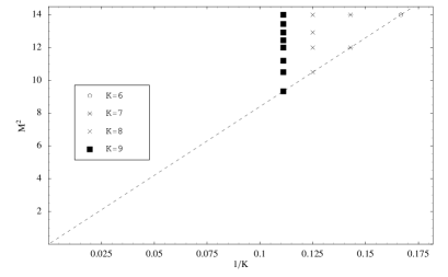
Figure 3: The lowest mass squared as a function of $1/K$ in the toy model.

At $K=7$ there are states at $M^{2}=14=84/6$ and 84/7; at $K=8$ there are states at $M^{2}=14$, 84/6.5, 84/7, and 84/8. It is straightforward to calculate the number of states with a mass squared less than any arbitrary $M^{2}$. We find

$$N(M^{2},K)=2^{(K-\frac{84}{M^{2}})}\Theta(14-M^{2})\Theta(K-6).$$ (10)

Thus at $K=6$ there is one massive state in the region $M^{2}\leq 14$, while at $K=8$ there are 4 states with $M^{2}\leq 14$. The total number of states at any $K$ is

$$N(K)=2^{(K-6)}\Theta(K-6).$$ (11)

The density of states can be calculated from $N(M^{2},K)$ and is

$$\rho(M^{2},K)=\frac{dN(M^{2},K)}{dM^{2}}=N(K)\tilde{\rho}(M^{2}),$$ (12)

where the reduced density of states [18] $\tilde{\rho}$ is just

$$\tilde{\rho}(M^{2})=2^{(6-\frac{84}{M^{2}})}\frac{84}{M^{4}}\ln(2)\Theta(14-M^{2}).$$ (13)

Clearly this is a peaked function that vanishes at $M^{2}=0$ and $\infty$. The location of the peak is set by the maximum mass allowed in the model, $M^{2}=14$. Of course one could rewrite the model for a very large maximum mass in order to model a larger range of masses. One finds that for masses much less than the mass at the peak of the density, it grows exponentially with $M$, suggesting that the model might have a Hagedorn temperature. The thermodynamics of a model displaying a Hagedorn temperature are discussed in [5].

3.3 Properties of the states

Since we solve for the wave functions in addition to the masses of the bound states, we can investigate the properties of the bound states discussed above. We already mentioned that the average number of partons in a bound state is higher for lower mass states. There is a four-fold degeneracy for all of the massive states, and the properties of these degenerate states can be very different. Here, we will look at properties such as the average number of partons and average number of fermions and their dependence on the symmetry sector to which the bound state belongs. The first useful observation is that the eight sectors of the theory contain different numbers of states. It is also interesting to note that different symmetry sectors have different numbers of massless states, and that the average parton and fermion numbers depend on the symmetry sector, as can be seen in Table 3.

$S$ $S+$ $S-$ $B$ $B+$ $B-$ $B+$ $B-$ $P$ $P+$ $P-$ $P+$ $P-$ $P+$ $P-$ $P+$ $P-$ Massless states? yes no no yes no yes yes no $K_{0}$: $\langle n\rangle$ 7.94 8.96 8.97 7.94 7.93 6.90 6.90 7.93 $K_{0}$: $\langle n_{f}\rangle$ 1.98 2.00 2.98 1.00 2.00 1.76 1.00 2.79 $K_{1}$: $\langle n\rangle$ 6.00 6.99 6.99 6.00 7.99 6.99 6.99 7.99 $K_{1}$: $\langle n_{f}\rangle$ 0.33 2.00 1.28 1.02 2.00 0.21 1.01 1.19

Table 3: Average parton number $\langle n\rangle$ and fermion number $\langle n_{f}\rangle$ in different sectors at resolution $K=9$, for the states in the sequences that begin at resolutions $K_{0}$ and $K_{1}$. Here $B+$ and $B-$ indicate the bosonic and fermionic sectors.

Looking at the zero-mass states, we find that they have either fermion number one or zero. Furthermore, we have states of very different length, ranging from the smallest to the largest possible number of partons in each sector.

It is interesting to consider the parton number of a bound state as a function of the harmonic resolution. As an example, we plot in Fig. 4 the average parton number of the lowest massive state that first appears at $K=3$ . We see that the parton number grows with $K$ in the sector with zero-mass states as well as in the sector without them.

(a)	(b)

Figure 4: Average parton number of the first massive state appearing at $K_{0}=3$ as a function of $K$ in (a) the bosonic $P-$, $S+$ sector (no zero-mass states) and (b) the bosonic $P+$, $S-$ sector (with zero-mass states). The lines are polynomial fits to the data.

The average number of partons in a bound state only tells part of the story. It is necessary to look also at the distribution of partons and ask how it changes with the resolution. We know that the states get longer and longer, but how this transition happens is not known. The parton distributions for a particular bound state are shown in Fig. 5. In Fig. 6 we plot fits to the probabilities of finding $n$ partons in this state as a function of the resolution. From the extrapolation, we find that the state consists of 48.7% three-parton, 41.4% five-parton, 9% seven-parton, and 0.9% nine-parton states. Note that these results of four independent extrapolations add up almost exactly to unity.

(a)	(b)

Figure 5: Parton number distribution for the first state appearing in the spectrum ($M_{3}^{2}(\infty)=21.7644$ in the bosonic $P-$, $S+$ sector). Plotted are the probabilities $p(n)$ for the state to have $n$ partons vs $n$, for resolutions (a) $K=12$ and (b) $K=17$.

Figure 6: Parton number distribution for the first state appearing in the spectrum ($M_{3}^{2}(\infty)=21.7644$ in the bosonic $P-$, $S+$ sector). Plotted are the probabilities $p(n)$ for the state to have $n$ partons vs. $1/K$. The curves (from top) are for $n=3,5,7,$ and $9$, respectively.

4 Counting states

4.1 Prime resolutions

It is very advantageous to know the exact number of states of a theory in a discrete approach like SDLCQ, because it may tell us something about the physics involved, e.g. massless eigenstates. We start by considering the case where the resolution is a prime number, which is the easiest situation. Because of the cyclicity of the color trace that defines the basis states, there is a many-to-one mapping from sequences of operators to states. First, we have to find the number of sequences of creation operators given $n$ species of particles at harmonic resolution $K$. To make the notation clear, consider the ${\cal N=}(1,1)$ case, where $n=2$. A typical sequence of operators at $K=13$ is

$$s^{\dagger}=a^{\dagger}(3)b^{\dagger}(1)b^{\dagger}(1)b^{\dagger}(3)a^{\dagger}(1)a^{\dagger}(4),$$ (14)

where $a^{\dagger}(k)$ creates a boson with longitudinal momentum fraction $k/K$ and $b^{\dagger}(k)$ creates a fermion. We encode this with the following 13 symbols

$$s^{\dagger}=\ a++\ b\ b\ b++\ a\ a++\;+,$$ (15)

with the “$+$“ symbol used to indicate an increase in the momentum above one; the notation suppresses the dagger symbols. The mapping between the two encodings is one-one and onto, so that their numbers must be the same. For a particular value of $K$, the encoding involves picking $K$ sequential choices from a set of three elements, with the restriction that the first choice cannot be the symbol “$+$”. Thus the number of sequences of operators for ${\cal N}=(1,1)$ is $2\times 3^{K-1}$. For a system with $n$ types of operators it is $n(n+1)^{K-1}$.

The number of states is less than the number of operator sequences. In our example, traces of the sequences of operators

$$s_{1}^{\dagger} = b^{\dagger}(1)b^{\dagger}(1)b^{\dagger}(3)a^{\dagger}(1)a^{\dagger}(4)a^{\dagger}(3),$$ (16)

$$s_{2}^{\dagger} = b^{\dagger}(1)b^{\dagger}(3)a^{\dagger}(1)a^{\dagger}(4)a^{\dagger}(3)b^{\dagger}(1),$$

$$s_{3}^{\dagger} = b^{\dagger}(3)a^{\dagger}(1)a^{\dagger}(4)a^{\dagger}(3)b^{\dagger}(1)b^{\dagger}(1),$$

would create the same state as $\hbox{Tr}[s^{\dagger}]$, because of the cyclicity of the trace. Thus, for the generic case, a sequence of $j$ operators will have $j-1$ redundant partners in the sequence listing. In other words, each sequence of $j$ partons should only contribute $1/j$ to the number of states. In symmetric cases, some of the rotations may not be distinct from the original sequence. In that case, the contribution should be greater than $1/j$. For $K$ prime, this only occurs for the sequence $a^{\dagger}(1)^{K}$. We will adjust the final result to account for this.

To calculate the number of distinct states, we define the following quantities:

• $n$ = number of types of operators (not counting “+”).

• $K$ = total number of momentum quanta.

• $j$ = number of partons (symbols other than $+$ in a sequence).

• $B(K,n,j)$ = number of sequences with given values for $K$, $n$, and $j$.

• $A(K,n,j)=\frac{B(K,n,j)}{j}=$ number of $j$-parton states, neglecting over-counting due to symmetry.

• $A(K,n)=\sum_{j=2}^{K}A(K,n,j)$ = number of states.

So, if $j=1$, then $B(K,n,j)=n$. The first symbol must be one of our $n$ types. The other $K-1$ symbols are all $+$. Note that this case will not be included in the list of states because we explicitly disallow operators where the momentum is $K$. In general, we must place one symbol from the $n$ types in the first position and $j-1$ in the other $K-1$ positions. These positions can be selected in $\left({\scriptsize\begin{array}[]{c}K-1\\ j-1\end{array}}\right)$ ways and the $j$ symbol choices selected in $n^{j}$ ways. Therefore, we have

$$B(K,n,j)=n^{j}\left(\begin{array}[]{c}K-1\\ j-1\end{array}\right).$$ (17)

To get the contribution to the number of states, we divide by $j$

$$A(K,n,j)=\frac{n^{j}}{j}\left(\begin{array}[]{c}K-1\\ j-1\end{array}\right)=\frac{n^{j}}{K}\left(\begin{array}[]{c}K\\ j\end{array}\right),$$ (18)

and to obtain the total, we sum over all contributions from the different parton numbers

$$A(K,n)=\sum_{j=2}^{K}\frac{n^{j}}{K}\left(\begin{array}[]{c}K\\ j\end{array}\right)=\frac{1}{K}\left[(1+n)^{K}-1-nK\right].$$ (19)

Thus, neglecting symmetry, we have a formula for the number of states as a function of the number of types of operators and the harmonic resolution $K$.

For $K$ prime, symmetry only plays a role when $j=K$. Rotations of a $K$-parton state, which has only one type of operator, leave the state unchanged. Each of the $n$, homogeneous, $K$-parton states contribute $1/K$ to the above formula and not one. Our corrected formula for the number of states is therefore

$$A(K,n)_{\rm prime}=\frac{1}{K}\left[(1+n)^{K}-(1+n)\right].$$ (20)

4.2 General resolutions

In this section we extend the above result to general $K$. We start by defining the functions

$$C(K,n,1)=n=2C_{f}(K,n,1)=2C_{b}(K,n,1),$$ (21)

$$C(K,n,j)=B(K,n,j)-\sum^{K}_{q>1,\,{\rm odd}}C(\frac{K}{q},n,\frac{j}{q}),$$

$$C_{f}(K,n,j)=B_{f}(K,n,j)-\sum^{K}_{q>1,\,{\rm odd}}C_{f}(\frac{K}{q},n,\frac{j}{q}),$$

$$C_{b}(K,n,j)=B_{b}(K,n,j)-\sum^{K}_{q>1,\,{\rm odd}}C_{b}(\frac{K}{q},n,\frac{j}{q}).$$

All functions $C(\frac{K}{q},n,\frac{j}{q})$ are taken to be zero when $K/q$ or $j/q$ is not an integer. The $f$ and $b$ subscripts indicate fermion or boson states, respectively. For example, $B_{f}(K,n,j)$ is the number of sequences of $K$ symbols with an odd number of fermions and $j$ partons. We then have $B_{f}(K,n,j)=B_{b}(K,n,j)=\frac{1}{2}B(K,n,j)$, where $B(K,n,j)$ is given in Eq. (17). Thus the $C$ functions are related by $C_{f}(K,n,j)=C_{b}(K,n,j)=\frac{1}{2}C(K,n,j)$.

The total number of fermionic states will be the sum over all odd $q\geq 1$ of fermionic states made from concatenations of sequences of length $K/q$

$$A_{f}(K,n,j)=\sum_{q,\,{\rm odd}}\frac{q}{j}C_{f}\left(\frac{K}{q},n,\frac{j}{q}\right).$$ (22)

The factor $q/j$ accounts for the $j/q$ sequences that map to the same state. The sum is restricted to odd concatenations because even concatenations would be bosons and are, in fact, rejected because of fermion statistics. Bosonic states can be made from concatenations of any number of bosonic subsequences.

We define the function $D(K,n,j)$ as the number of symbol sequences of length $K$ that are not concatenations of smaller sequences. We have the relation that a sequence counted in $C(K,n,j)$ may be non-symmetric or it may be a concatenation of $2^{l}$ smaller sequences. If it were a concatenation of $2^{l}q$ smaller sequences, where $q$ is odd, it would have been included in $C(K/q,n,j/q)$. Thus we have

$$D(K,n,j)=C(K,n,j)-C\left(\frac{K}{2},n,\frac{j}{2}\right).$$ (23)

Since $D_{f}(K,n,j)=C_{f}(K,n,j)$, we find

$$D_{b}(K,n,j)=C_{b}(K,n,j)-C\left(\frac{K}{2},n,\frac{j}{2}\right)=C_{b}(K,n,j)-2C_{b}\left(\frac{K}{2},n,\frac{j}{2}\right).$$ (24)

Now we are ready to calculate the number of bosonic states

$$A_{b}(K,n,j) = \sum_{q}\frac{q}{j}D_{b}\left(\frac{K}{q},n,\frac{j}{q}\right)$$

$$= \sum_{q}\frac{q}{j}\left[C_{b}\left(\frac{K}{q},n,\frac{j}{q}\right)-2C_{b}\left(\frac{K}{2q},n,\frac{j}{2q}\right)\right]=\sum^{K}_{q,\,{\rm odd}}\frac{q}{j}C_{b}\left(\frac{K}{q},n,\frac{j}{q}\right).$$

This result proves that the number of fermions and bosons is equal at each resolution $K$ and parton number $j$. We can sum the total number of states over all $j>1$

$$A_{f}(K,n)=\sum_{j}\sum_{q,\,{\rm odd}}\frac{q}{j}C_{f}\left(\frac{K}{q},n,\frac{j}{q}\right)-A_{f}(K,n,1)=\sum_{q,\,{\rm odd}}A^{\prime}_{f}\left(\frac{K}{q},n\right)-\frac{n}{2},$$ (26)

where we have defined the non-symmetric state number function

$$A^{\prime}_{f}(K,n) \equiv \sum_{j}\frac{1}{j}C_{f}(K,n,j)=\sum_{j}\frac{1}{j}B_{f}(K,n,j)-\sum_{q>1,\,{\rm odd}}\sum_{j}\frac{1}{j}C_{f}\left(\frac{K}{q},n,\frac{j}{q}\right)$$ (27)

$$= \sum_{j}\frac{1}{j}B_{f}(K,n,j)-\sum_{q>1,\,{\rm odd}}\frac{1}{q}A^{\prime}_{f}\left(\frac{K}{q},n\right)$$

$$= \frac{(1+n)^{K}-1}{2K}-\sum_{q>1,\,{\rm odd}}\frac{1}{q}A^{\prime}_{f}\left(\frac{K}{q},n\right).$$

The result for $A_{b}(K,n)$ is evidently the same, and we have $A(K,n)=2A_{f}(K,n)$.

4.3 Symmetry sectors

There are several symmetries of the Hamiltonian which can be used to reduce the numerical effort by block diagonalization. Each block corresponds to a distinct symmetry sector of the theory. In the ${\cal N}=(1,1)$ theory these are supersymmetry, $S$ symmetry (5), and parity (6). Thus the ${\cal N}=(1,1)$ theory has eight symmetry sectors. The supercharge $Q^{-}$ changes the fermion number by one, taking a sector to its image sector. In many cases the image sector will have fewer states, which requires the existence of massless states in the initial sector, since massless states are annihilated by $Q^{-}$. Knowledge of the number of states in each sector can provide a lower bound on the number of massless states.

The ${\cal N}=(2,2)$ theory has an additional $Y$ symmetry:

$$Y:a_{1}(k^{+})\leftrightarrow a_{2}(k^{+}),\qquad b_{1}(k^{+})\rightarrow b_{1}(k^{+}),\qquad b_{2}(k^{+})\rightarrow-b_{2}(k^{+}).$$ (28)

The eight sectors determined by supersymmetry, parity, and $S$-symmetry are each split exactly in half by this additional symmetry. Thus the minimum number of massless states is not changed if $Y$ symmetry is present.

In this section, we will provide formulas for the numbers of states in the four supersymmetry and parity sectors. We will show that the total number of positive and negative eigenvalues for the $Y$ symmetry are equal. Then we shall show that the $SY$ operation has the same number of positive and negative eigenvalues in each of the four supersymmetry and parity sectors and calculate the number of additional positive eigenvectors that the $S$ symmetry possesses. We then apply the results to find the number of states for each sector. Finally, we apply the count in each sector to the problem of counting massless states.

4.3.1 Supersymmetry and parity

From the previous section we know that

$$A_{fo}(K,n)=A_{bo}(K,n)\qquad\mbox{and}\qquad A_{fe}(K,n)=A_{be}(K,n),$$ (29)

where the subscripts denote fermion and boson sectors and odd and even parton numbers, respectively. $A_{fo}$ and $A_{be}$ count states with even parity and are taken into each other by $Q^{-}$ which changes the fermion number of a state by one and changes the boson number by two or none. In order to compare numbers of states, we need therefore to relate the counts of even and odd-parton states.

We consider the number of fermionic sequences $B_{f}(K,n,j)=\frac{1}{2}B(K,n,j)$; see Eq. (17). In this function, the power of $n$ is even if and only if $j$ is even. Next we consider the number of non-symmetric fermionic sequences, given in Eq. (4.2). Since $q$ is restricted to odd values, $j/q$ will be even (odd) when $j$ is even (odd) and therefore, by induction, $B_{f}(K,n,j)$ will have even (odd) powers of $n$ when $j$ is even (odd). In fact, the even-odd dependence carries through the whole calculation. Therefore, we have

$$A_{be}(K,n)=A_{fe}(K,n)=\frac{1}{2}\left[A_{f}(K,n)+A_{f}(K,-n)\right],$$ (30)

$$A_{bo}(K,n)=A_{fo}(K,n)=\frac{1}{2}\left[A_{f}(K,n)-A_{f}(K,-n)\right].$$

Thus we have separated the states into four sectors, and we know the numbers of states in each sector.

4.3.2 $Y$ symmetry

For ${\cal N}=(2,2)$ SYM theory, the situation is different, because our basis states are not all eigenstates of the additional $Y$ symmetry. Most Fock states $|\psi\rangle$ are mapped onto distinct states $Y|\psi\rangle$ by the symmetry. A $Y$-even (odd) eigenvector will then be of the form $|\psi\rangle\pm Y|\psi\rangle$. Thus, if each state had distinct partner under $Y$, the space would clearly split exactly in half between states with positive and negative eigenvalues. However, there are states such that $Y|\psi\rangle=\pm|\psi\rangle$, and they must be counted before showing that the space does indeed split exactly in half.

There are two ways that a Fock state can be an eigenstate of $Y$. The first is for it to have no bosons. In that case, the $Y$ eigenvalue is determined by the number of $b_{2}^{\dagger}$ operators. The second is for the state to have the form $\hbox{Tr}\left[(s^{\dagger}\bar{s}^{\dagger})^{q}\right]|0\rangle$, where $s^{\dagger}$ is a sequence of creation operators, $\bar{s}^{\dagger}$ is the sequence obtained from $s^{\dagger}$ by interchanging $a_{1}^{\dagger}$ and $a_{2}^{\dagger}$, and $q$ is a positive integer. The sequences of this type will have an even number of $b_{2}^{\dagger}$ operators. Their $Y$ eigenvalue is determined by the fermion number of $s^{\dagger}$, unless $s^{\dagger}=\bar{s}^{\dagger}$, which will occur for purely fermionic sequences.

The problem of counting the positive and negative $Y$ eigenvalues among the states that have no bosons in the case $n=4$ is almost equivalent to the counting of fermion and boson states in the case $n=2$. We map the $n=4$ sequences to $n=2$ according to the replacements $b_{1}^{\dagger}\rightarrow a^{\dagger}$ and $b_{2}^{\dagger}\rightarrow b^{\dagger}$. However, due to fermion statistics, there is not a perfect one-to-one correspondence between $n=2$ states and purely fermionic $n=4$ states. In particular, $n=4$ states created from an even number of even parton number subsequences, which each have an odd number of $b_{2}^{\dagger}$ operators, will have no corresponding $n=2$ state. For resolution, $K$, and $j$ partons, the count of these states, which all have positive $Y$ eigenvalue, is

$$\delta Y_{1+}(K,j)=\sum_{q,\,{\rm even}}\frac{q}{j}C_{f}\left(\frac{K}{q},2,\frac{j}{q}\right).$$ (31)

Also, some $n=2$ boson states have no corresponding $n=4$ states because they would consist of an even number of odd parton number subsequences. The corresponding $n=2$ states of this latter type have as their total

$$\delta Y_{1-}(K,j)=\sum_{\scriptsize\begin{array}[]{c}j/q,\,{\rm odd}\\ q,\,{\rm even}\end{array}}\frac{q}{j}D\left(\frac{K}{q},2,\frac{j}{q}\right)=\sum_{\scriptsize\begin{array}[]{c}j/q,\,{\rm odd}\\ q,\,{\rm even}\end{array}}\frac{q}{j}\left[C\left(\frac{K}{q},2,\frac{j}{q}\right)-C\left(\frac{K}{2q},2,\frac{j}{2q}\right)\right].$$ (32)

The last term, $C\left(\frac{K}{2q},2,\frac{j}{2q}\right)$, is zero, because $j/q$ is odd and therefore not divisible by 2.

The difference between (31) and (32) gives the difference between $n=4$ purely fermionic positive-$Y$ states and $n=2$ bosonic states. Since $n=2$ has an equal number of boson and fermion states, the net difference between numbers of positive and negative $Y$ eigenvalues for purely fermionic states with $j$ partons is

$$\delta Y_{1+}(K,j)-\delta Y_{1-}(K,j) = \sum_{q,\,{\rm even}}\frac{q}{j}C_{f}\left(\frac{K}{q},2,\frac{j}{q}\right)-\sum_{\scriptsize\begin{array}[]{c}j/q,\,{\rm odd}\\ q,\,{\rm even}\end{array}}\frac{q}{j}2C_{f}\left(\frac{K}{q},2,\frac{j}{q}\right)$$ (35)

$$= \sum_{q,\,{\rm even}}(-1)^{j/q}\frac{q}{j}C_{f}\left(\frac{K}{q},2,\frac{j}{q}\right).$$ (36)

We next consider the contribution from $Y$ eigenstates of the form $\hbox{Tr}\left[(s^{\dagger}\bar{s}^{\dagger})^{q}\right]|0\rangle$. To avoid duplication, we count only those sequences $s^{\dagger}\bar{s}^{\dagger}$ that cannot be further subdivided as $(s^{\prime\dagger}\bar{s}^{\prime\dagger})^{(2r+1)}$ for some sequence $s^{\prime\dagger}$ and some integer $r>0$. For $j$ partons and resolution $K$, the number of such states is $\frac{1}{2}\frac{2q}{j}C\left(\frac{K}{2q},n,\frac{j}{2q}\right)$, where we have included a factor of 1/2 to account for the fact that $\hbox{Tr}\left[(s^{\dagger}\bar{s}^{\dagger})^{q}\right]|0\rangle$ is not distinct from $\hbox{Tr}\left[(\bar{s}^{\dagger}s^{\dagger})^{q}\right]|0\rangle$. Since $C_{b}=C_{f}$, there are equal numbers of positive and negative eigenvalues among these states. However, the purely fermionic states have already been counted and must be removed from this second contribution. They are subtracted from the positive count when $j/2q$ is even and from the negative count when it is odd. Each count is done as before, by mapping to $n=2$ states, and the net contribution is

$$\delta Y_{2+}(K,j)-\delta Y_{2-}(K,j)=-\sum_{q\geq 1}(-1)^{j/2q}\frac{q}{j}C\left(\frac{K}{2q},2,\frac{j}{2q}\right).$$ (37)

Since $C=2C_{f}$, this exactly cancels $\delta Y_{1+}(K,j)-\delta Y_{1-}(K,j)$.

4.3.3 $S$ and $SY$ symmetry

The $S$ symmetry swaps the color indices of the operators and multiplies each by $-1$. It is equivalent to reversing the order of the operators in a state and multiplying by a sign $(-1)^{j}(-1)^{\frac{n_{f}(n_{f}-1)}{2}}$, where $j$ is the number of partons and $n_{f}$ is the number of fermions in the state. In this section we look for Fock states that are eigenstates of $S$ or, for the ${\cal N}=(2,2)$ theory, of $SY$. We look for the difference between the numbers of positive and negative eigenvalues of these two operators. Most of these eigenvectors come in pairs, one with positive and one with negative eigenvalue but with equal parton number and the same parity of fermion number. We only need to count the ones that do not come in pairs. For Fock states $|\psi\rangle$ which are not eigenstates we again form combinations $|\psi\rangle\pm S|\psi\rangle$ or $|\psi\rangle\pm SY|\psi\rangle$ as pairs of eigenstates with opposite eigenvalues. For Fock states which are eigenstates, we find only pairs with opposite eigenvalues except for two-parton states.

We can see this by considering even and odd parton number separately. For odd parton number, we rotate the sequence of symbols to the form $s^{\dagger}x^{\dagger}\bar{s}_{R}^{\dagger}$ where the sequence $s_{R}^{\dagger}$ is the reversal of $s^{\dagger}$ and $\bar{s}_{R}^{\dagger}=s_{R}^{\dagger}$ or $Ys_{R}^{\dagger}$, depending on whether we are considering the $S$ symmetry or the $SY$ symmetry, and $x^{\dagger}$ is a single operator satisfying $Yx^{\dagger}=\pm x^{\dagger}$ under $SY$ symmetry. By changing the first operator in $s^{\dagger}$ from boson to fermion, we change the fermion number by two and the sign of $S$ while changing neither parton number nor fermion-number parity. Thus states of this form do come in pairs.

For even parton number the argument is more complicated, and we just give a sketch. There is a two-to-one map between sequences of operators of the types $s^{\dagger}\bar{s}_{R}^{\dagger}$ and $x^{\dagger}s^{\dagger}y^{\dagger}\bar{s}_{R}^{\dagger}$ and basis states that are eigenvalues of $S$ or $SY$, where $s^{\dagger}$ and $\bar{s}_{R}^{\dagger}$ are subsequences and $x^{\dagger}$ and $y^{\dagger}$ are single operators, as before. Again, we can flip the first operator in $s^{\dagger}$ from fermion to boson to swap the sign of the $S$ or $SY$ eigenvalue. Some states are absent due to fermion statistics, but they also come in pairs.

The argument does not apply to two-parton states, which we now handle explicitly. All two-parton basis states are eigenstates of $S$ with positive eigenvalue. All $S$ does in this case is swap the dummy summation indices. The number of two-parton fermionic states is $(\frac{n}{2})^{2}(K-1)$. This comes from two choices of which fermion and boson to include and $K-1$ choices as to how to apportion the momentum between the two operators. The number for two-parton bosonic states is the same.

The two-parton Fock states that are eigenstates of $SY$ are listed in Table 4; positive and negative eigenvalues appear there in equal numbers. The two-parton fermion states have exactly one boson operator and cannot be eigenstates of $Y$. The numbers of positive and negative eigenvalues of $SY$ are therefore equal.

number of states State $SY$ $K$ even $K$ odd $\hbox{Tr}\left[a_{1}^{\dagger}(K/2)a_{2}^{\dagger}(K/2)\right]|0\rangle$ 1 1 0 $\hbox{Tr}\left[b_{1}^{\dagger}(k)b_{2}^{\dagger}(K-k)\right]|0\rangle$ $-1$ $K-1$ $K-1$ $\hbox{Tr}\left[b_{1}^{\dagger}(k)b_{1}^{\dagger}(K-k)\right]|0\rangle$ 1 $K/2-1$ $(K-1)/2$ $\hbox{Tr}\left[b_{2}^{\dagger}(k)b_{2}^{\dagger}(K-k)\right]|0\rangle$ 1 $K/2-1$ $(K-1)/2$

Table 4: Two-parton Fock states that are eigenstates of $SY$.

The number of $S+$ and $S-$ eigenstates is equal for odd parity and even or odd fermion numbers, but in the even-parity fermion and boson sectors, the number of $S+$ eigenstates is greater than the number of $S-$ eigenstates by $(\frac{n}{2})^{2}(K-1)$.

4.3.4 Results

We label the $Y$ and $S$ symmetry sectors by additional letters $y^{\pm}$ and $s^{\pm}$, e.g. $A_{bey^{+}}+A_{bey^{-}}=A_{be}$. It is obvious that no odd-parity Fock state, with its odd number of bosons, can be an eigenstate of $Y$ or $SY$; therefore, $Y$ and $SY$ eigenvalues occur in equal numbers in each such sector, and we have

$$A_{fes^{+}y^{+}}=A_{fes^{+}y^{-}}\qquad\mbox{and}\qquad A_{fes^{-}y^{+}}=A_{fes^{-}y^{-}},$$ (38)

$$A_{bos^{+}y^{+}}=A_{bos^{+}y^{-}}\qquad\mbox{and}\qquad A_{bos^{-}y^{+}}=A_{bos^{-}y^{-}}.$$

Fermionic states with an odd number of partons can be eigenstates, but they come in pairs related by the exchange of $b_{1}$ and $b_{2}$. Therefore, the counts in these sectors must also be equal:

$$A_{fos^{+}y^{+}}=A_{fos^{+}y^{-}}\qquad\mbox{and}\qquad A_{fos^{-}y^{+}}=A_{fos^{-}y^{-}}.$$ (39)

The bosonic even-parity sectors are all that remain to be considered. Since we have $A_{y^{+}}=A_{y^{-}}$, the totals for the bosonic even-parton sector must also be equal:

$$A_{bey^{+}}=A_{bey^{-}}.$$ (40)

Furthermore, since $SY$ has an equal number of positive and negative eigenvalues, we have

$$A_{bes^{+}y^{+}}+A_{bes^{-}y^{-}}=A_{bes^{+}y^{-}}+A_{bes^{-}y^{+}},$$ (41)

and, therefore,

$$A_{bes^{+}y^{+}}=A_{bes^{+}y^{-}}\qquad\mbox{and}\qquad A_{bes^{-}y^{+}}=A_{bes^{-}y^{-}}.$$ (42)

For eigenstates of $S$ alone, we have

$$A_{bes^{+}}-A_{bes^{-}}=A_{fes^{+}}-A_{fes^{-}} = \frac{n^{2}}{4}(K-1)$$ (43)

$$A_{bos^{+}}-A_{bos^{-}}=A_{fos^{+}}-A_{fos^{-}} = 0.$$

Thus, from Eq. (30) we obtain

$$A_{bes^{+}}(K,n)=A_{fes^{+}}(K,n) = \frac{1}{4}\left\{A_{f}(K,n)+A_{f}(K,-n)+\frac{n^{2}}{2}(K-1)\right\},$$ (44)

$$A_{bes^{-}}(K,n)=A_{fes^{-}}(K,n) = \frac{1}{4}\left\{A_{f}(K,n)+A_{f}(K,-n)-\frac{n^{2}}{2}(K-1)\right\},$$

$$A_{bos^{+}}(K,n)=A_{fos^{+}}(K,n) = \frac{1}{4}\left\{A_{f}(K,n)-A_{f}(K,-n)\right\}$$

$$= A_{bos^{-}}(K,n)=A_{fos^{-}}(K,n).$$

We present the results for the numbers of states in the different sectors for the ${\cal N}=(1,1)$ and ${\cal N}=(2,2)$ theories in Tables 5 and 6, respectively.

$K$	$A_{bes^{+}}$	$A_{bos^{+}}$	$A_{bes^{-}}$
2	1	0	0
3	2	1	0
4	4	2	1
5	8	6	4
6	18	15	13
7	42	39	36
8	106	102	99
9	278	274	270
10	743	738	734
11	2018	2013	2008
12	5543	5537	5532
13	15336	15330	15324
14	42712	42705	42699
15	119586	119579	119572
16	336310	336302	336295
17	949568	949560	949552
18	2690439	2690430	2690422
19	7646466	7646457	7646448
20	21792414	21792404	21792395

Table 5: Number of states in the different symmetry sectors for the ${\cal N}=(1,1)$ theory. Recall that $A_{bes^{\pm}}=A_{fes^{\pm}}$ and $A_{bos^{+}}=A_{fos^{+}}=A_{bos^{-}}=A_{fos^{-}}$.

$K$	$A_{bes^{+}}$	$A_{bos^{+}}$	$A_{bes^{-}}$
2	4	0	0
3	8	6	0
4	28	16	16
5	80	84	64
6	352	310	332
7	1368	1434	1344
8	6220	6000	6192
9	26872	27404	26840
10	122828	121332	122792
11	552872	556878	552832
12	2548704	2537606	2548660
13	11722224	11752860	11722176
14	54538408	54452970	54538356
15	254193656	254432786	254193600
16	1192429228	1191756592	1192429168
17	5608899392	5610798480	5608899328
18	26493643916	26488263020	26493643848
19	125475816264	125491109142	125475816192
20	596068240212	596024655364	596068240136

Table 6: Number of states in the different symmetry sectors for the ${\cal N}=(2,2)$ theory. Recall that $A_{bes^{\pm}}=A_{fes^{\pm}}$ and $A_{bos^{+}}=A_{fos^{+}}=A_{bos^{-}}=A_{fos^{-}}$.

How can we make use of these results? Since the supercharge $Q^{-}$ maps one symmetry sector to another, we can conclude that if one sector has $r$ more states than the other, then the Hamiltonian $P^{-}\propto(Q^{-})^{2}$ has at least $r$ massless states in that sector.

In the ${\cal N}=(1,1)$ theory, we can calculate $A_{f}(K,-2)$ explicitly. From Eq. (27) we know that $A^{\prime}_{f}(1,-2)=-1$ and $A^{\prime}_{f}(2,-2)=0$. Then for $A^{\prime}_{f}(2K,-2)$ the recursive sum yields zero. The net result is the same for $A^{\prime}_{f}(2K+1,-2)$:

$$A^{\prime}_{f}(2K+1,-2)=\frac{1}{4K+2}\left\{[1+(-2)]^{2K+1}-1-2A^{\prime}_{f}(1,-2)\right\}=0.$$ (45)

From these and Eq. (26) we have

$$A_{f}(2K+1,-2) = A^{\prime}_{f}(2K+1,-2)+A^{\prime}_{f}(1,-2)-(-1)=0,$$ (46)

$$A_{f}(2K,-2) = A^{\prime}_{f}(2K,-2)-(-1)=1.$$

This means that for the ${\cal N}=(1,1)$ case, the bosonic and fermionic parity-even and $S$-even sectors must have $(K-1)/2$ (for odd $K$) or $K/2$ (for even $K$) more states than their parity-odd counterparts. Likewise, the bosonic and fermionic parity-odd and $S$-odd sectors must have $(K-1)/2$ (odd $K$) or $K/2-1$ (even $K$) more states than their parity-even counterparts. The minimum number of massless states is therefore $2(K-1)$, regardless of whether the resolution $K$ is even or odd.

5 Discussion

In this paper we discussed a number of properties of ${\cal N}=(1,1)$ super Yang–Mills theory in two dimensions at large $N_{c}$ in a SDLCQ approach. We found the low-energy bound-state spectrum in each of the symmetry sectors and extrapolated the spectrum to obtain the continuum masses. Although convergence is fast and approximately linear, we were careful to push our numerical calculations to large resolution $K$. We found that this spectrum exhibits an interesting distribution of masses. We explained this pattern and discussed how one can understand it by constructing a toy model, that one might use to approximate the actual spectrum. We looked at some of the properties of a number of these bound states in detail.

Finally, we considered the numbers of states in the Fock basis in a SDLCQ approximation. Obviously, one would like to know how many basis states one will encounter before one attempts a numerical approximation, since, in an actual SDLCQ calculation, we solve the problem separately in each symmetry sector. We calculated the number of states in each symmetry sector algebraically. It is useful to know which sector has the smallest number of states, because this sector will generally have the smallest number of massless states, which makes it the simplest one to solve numerically. Our calculation showed that the number of fermion states is exactly equal to the number of boson states. This represents part of the answer as to why the SDLCQ approximation is exactly supersymmetric.

The results presented in this paper nearly complete the solution of the ${\cal N}=(1,1)$ super Yang–Mills theory in two dimensions. In previous papers [4, 5] we had calculated the thermodynamics of the model and the behavior of the correlator of the energy momentum tensors and the distribution function of some of the bound states. We have discussed the spectrum of the theory and the counting of its states in this paper. In terms of the general behavior of this theory, little more than the analysis of the massless states remains to be done.

References

- [1] F. Antonuccio, O. Lunin, and S. Pinsky, Phys. Rev. D 59, 085001 (1999).
- [2] P. Haney, J. R. Hiller, O. Lunin, S. Pinsky, and U. Trittmann, Phys. Rev. D 62, 075002 (2000).
- [3] J. R. Hiller, S. Pinsky, and U. Trittmann, Phys. Rev. D 64, 105027 (2001).
- [4] F. Antonuccio, O. Lunin, and S. S. Pinsky, Phys. Lett. B 429, 327 (1998); Phys. Rev. D 58, 085009 (1998).
- [5] J. R. Hiller, Y. Proestos, S. Pinsky, and N. Salwen, Phys. Rev. D 70, 065012 (2004).
- [6] Y. Matsumura, N. Sakai, and T. Sakai, Phys. Rev. D 52, 2446 (1995).
- [7] O. Lunin and S. Pinsky, AIP Conf. Proc. 494, 140 (1999).
- [8] H. C. Pauli and S. J. Brodsky, Phys. Rev. D 32, 1993 (1985); Phys. Rev. D 32, 2001 (1985).
- [9] S.J. Brodsky, H.-C. Pauli, and S.S. Pinsky, Phys. Rep. 301, 299 (1998).
- [10] A. G. Cohen, D. B. Kaplan, E. Katz, and M. Unsal, JHEP 0308, 024 (2003); 0312, 031 (2003); A. Feo, Nucl. Phys. Proc. Suppl. 119, 198 (2003); Mod. Phys. Lett. A 19, 2387 (2004); I. Montvay, Nucl. Phys. B 466, 259 (1996).
- [11] F. Antonuccio, O. Lunin, S. Pinsky, and S. Tsujimaru, Phys. Rev. D 60, 115006 (1999).
- [12] J. S. Rozowsky and C. B. Thorn, Phys. Rev. Lett. 85, 1614 (2000).
- [13] S. Salmons, P. Grange, and E. Werner, Phys. Rev. D 65, 125014 (2002).
- [14] T. Heinzl, arXiv:hep-th/0310165.
- [15] A. Harindranath, L. Martinovic, and J. P. Vary, Phys. Lett. B 536, 250 (2002); V. T. Kim, G. B. Pivovarov, and J. P. Vary, Phys. Rev. D 69, 085008 (2004).
- [16] D. Chakrabarti, A. Harindranath, L. Martinovic, and J. P. Vary, Phys. Lett. B 582, 196 (2004).
- [17] D. Kutasov, Nucl. Phys. B 414, 33 (1994).
- [18] O. Lunin and S. Pinsky, Phys. Rev. D 63, 045019 (2001).