NUB-TH-3252
MIT-CTP-3567
hep-th/0411201

Hierarchically Split Supersymmetry
with Fayet-Iliopoulos D-terms
in String Theory

Abstract

We show that in string theory or supergravity with supersymmetry breaking through combined F-terms and Fayet-Iliopoulos D-terms, the masses for charged scalars and fermions can be hierarchically split. The mass scale for the gauginos and higgsinos of the MSSM is controlled by the gravitino mass $m_{3/2}$, as usual, while the scalars get extra contributions from the D-terms of extra abelian $U(1)$ factors, which can make them much heavier. The vanishing of the vacuum energy requires that their masses lie below $\sqrt{m_{3/2}M_{\rm Pl}}$, which for $m_{3/2}={\cal O}({\rm TeV})$ sets a bound of $10^{10-13}\,{\rm GeV}$. Thus, scalars with non-vanishing $U(1)$ charges typically become heavy, while others remain light, producing a spectrum of scalars with masses proportional to their charges, and therefore non-universal. This is a modification of the split supersymmetry scenario, but with a light gravitino. We discuss how Fayet-Iliopoulos terms of this size can arise in orientifold string compactifications with D-branes. Furthermore, within the frame work of D-term inflation, the same vacuum energy that generates the heavy scalar masses can be responsible for driving cosmological inflation.

1 Introduction

The conventional approach to supersymmetry breaking in models of supergravity (SUGRA) is to assume some form of spontaneous breaking in a hidden sector, mediated to the visible sector with contains the MSSM via gravitational interactions [1]. The overall mass scale is then set by the gravitino mass $m_{3/2}$, and all other masses for squarks, sleptons, gauginos and higgsinos come out roughly proportional to it, by demanding the cancellation of the vacuum energy. Low energy supersymmetry, as required by a natural explanation of the Higgs potential, fixes $m_{3/2}$ to the electro-weak scale. Now, recently it was argued [2] that the fine tuning problem of the Higgs mass may be insignificant compared to the fine tuning of the cosmological constant, and that an anthropic selection mechanism (see e.g. [3]) may then involve actual fine tuning of MSSM parameters. The mass pattern that was proposed under the name of split supersymmetry [4] has all the MSSM fermions at the electro-weak scale, whereas all scalars, except for the one fine tuned Higgs doublet, get ultra-heavy at a high mass scale. This scenario has attracted some attention recently [5]. More concretely, the challenge for model building is to keep the gauginos and higgsinos light, while letting the scalars become very heavy. The motivation for this originates from supersymmetric grand unification, even without low energy supersymmetry in the usual sense, and the model is designed to keep the merits of gauge coupling unification as in the MSSM. Here, we pursue the perspectives of such patterns in the mass spectrum in the context of SUGRA and string theory models, based on the paradigm of spontaneous breaking in a hidden sector.

Given the above mentioned relations that govern gravity mediated supersymmetry breaking, it seems very hard to achieve hierarchically split mass scales. If all masses are proportional to $m_{3/2}$, there is no room for flexibility. There is however a loophole to the argument, which has not so far been explored in the conventional approach in any depth, probably because it quickly leads to large masses, which were thought unacceptable. It consists of assuming not only auxiliary F-terms but also D-terms to be generated. In global supersymmetry, this is well known under the label of supersymmetry breaking mediated by an anomalous $U(1)$, where large masses can be avoided [6, 7], as will be seen later. The mechanism basically adds a Fayet-Iliopoulos (FI) term for an extra anomalous $U(1)$ gauge symmetry, independent of the F-terms which may also be present. In local supergravity, the two contribute both to the vacuum energy, and thus get tied together at roughly the same scale. Still, the contribution to scalar masses can be very different, since the F-terms are mediated via gravity, while the D-terms are mediated via gauge interactions, which opens up the possibility to have hierarchically split mass scales, splitting scalars charged under the relevant $U(1)$, from all other fields, i.e. gauginos, higgsinos as well as scalars not charged under the relevant $U(1)$’s. This is not quite along the lines of high scale supersymmetry breaking, as advocated in split supersymmetry, where the gravitino mass itself was assumed at the high scale, and the main difficulty lies in keeping the gauginos and higgsinos lighter than $m_{3/2}$. Instead, we propose extra contributions to the masses of charged scalars, which make them heavier than $m_{3/2}$, while the fermions including the gravitino remain light.

The purpose of this paper is to study the confluence of this combined approach with F- and D-terms in supergravity and string theory models. By this we mean that we assume that some hidden sector dynamics generates F- and D-terms at some scale of supersymmetry breaking, but we do not present a full dynamical model, how this happens. Instead, we analyze the various scenarios that can emerge in the visible sector, and in particular identify classes of models which generically lead to hierarchically split mass scales.

1.1 FI-terms in global supersymmetry

In many models of grand unification, compactification of higher dimensional supergravity or string theory, the minimal gauge symmetries that can be achieved at low energies involve various extra abelian $U(1)$ gauge factors beyond the Standard Model gauge group, i.e. the total gauge symmetry is $SU(3)_{C}\times SU(2)_{L}\times U(1)^{n}$, where among the $U(1)$ there is also the hypercharge. In string theory it often happens that some of the extra factors are actually anomalous, the anomaly being canceled by a (generalized) Green-Schwarz (GS) mechanism, in which the gauge boson develops a Stueckelberg mass and decouples (see e.g. [10]). In any case, it is then permissible to add FI-terms $\xi_{a}D_{a}$ to the supersymmetric Lagrangian, one for each $U(1)_{a}$. The D-term potential in global supersymmetry is

$${\cal V}_{D}~{}=~{}\sum_{a}\frac{g_{a}^{2}}{2}D_{a}^{2}=\sum_{a}\frac{g_{a}^{2}}{2}\Big{(}\sum_{i}Q_{a}^{i}|\tilde{f}_{i}|^{2}+\xi_{a}\Big{)}^{2}$$ (1)

and thus $\xi_{a}>0$ leads to the formation of a condensate for at least some field $\tilde{f}_{i}$ of negative charge $Q_{a}^{i}<0$. This breaks the gauge symmetry spontaneously, but supersymmetry can be restored at the minimum if $\langle D_{a}\rangle=0$. In the MSSM it is usually assumed that the FI-term of the hypercharge is absent or very small, and does not play a role in the Higgs potential.

Whenever the auxiliary field obtains a non-vanishing expectation value $\langle D_{a}\rangle\not=0$, supersymmetry is broken, and mass terms are generated for all the charged scalars,

$$m_{i}^{2}~{}=~{}\sum_{a}g_{a}^{2}Q_{a}^{i}\langle D_{a}\rangle\ ,$$ (2)

where it is now assumed that the charges are positive for the MSSM fields, to avoid breaking of the Standard Model gauge symmetries. This scenario can be achieved in a global supersymmetric model with a single extra $U(1)_{X}$ by adding two scalars $\phi^{\pm}$ to the MSSM, singlets under $SU(3)_{c}\times SU(2)_{L}\times U(1)_{Y}$, but with charges $\pm 1$ under $U(1)_{X}$ [6]. The crucial ingredient is an interaction in the superpotential of the form

$$W_{\pm}=m\phi^{+}\phi^{-}\ .$$ (3)

Minimizing the full potential

$${\cal V}=m^{2}\left(|\phi^{+}|^{2}+|\phi^{-}|^{2}\right)+\frac{g_{X}^{2}}{2}\Big{(}\sum_{i}Q_{X}^{i}|\tilde{f}_{i}|^{2}+|\phi^{+}|^{2}-|\phi^{-}|^{2}+\xi_{X}\Big{)}^{2}$$ (4)

drives the fields to

$$\langle\phi^{+}\rangle=0\ ,\quad\langle\phi^{-}\rangle^{2}=\xi_{X}-\frac{m^{2}}{g_{X}^{2}}\ ,$$ (5)

and

$$\langle D_{X}\rangle~{}=~{}\frac{m^{2}}{g_{X}^{2}}\ ,\quad\langle F_{\phi^{+}}\rangle~{}=~{}m\sqrt{\xi_{X}}+\,\cdots\ .$$ (6)

Gaugino masses may originate from higher dimensional operators, and are suppressed by powers of $M_{\rm Pl}$,

$$m_{\lambda}~{}\sim~{}\frac{1}{M_{\rm Pl}^{2}}\langle F_{\phi^{+}}\phi^{-}+F_{\phi^{-}}\phi^{+}\rangle~{}\sim~{}m\frac{\xi_{X}}{M_{\rm Pl}^{2}}\ .$$ (7)

Assuming $m\sim{\cal O}({\rm TeV})$ and $\xi\sim{\cal O}(M_{\rm Pl}^{2})$ on gets masses at the electro-weak scale. Depending on the precise scale and the charges of the MSSM scalars under the extra $U(1)_{X}$, these contributions to their masses can be very important in the soft breaking Lagrangian. A central point to notice here is the fact that the masses that follow from the FI-terms are directly proportional to the expectation values of the auxiliary $D_{a}$ fields, they are mediated by the anomalous $U(1)_{X}$, whereas the masses induced via the F-terms are suppressed by $M_{\rm Pl}$ through their mediation by gravity. The function of the extra fields $\phi^{\pm}$ lies in absorbing the potentially large FI parameter $\xi_{a}$, such that $\langle D_{a}\rangle^{1/2}\sim{\cal O}({\rm TeV})$, consistent with the standard scenario of superpartner masses at the electro-weak scale.

We will discuss this type of model and its modifications in the frame work of supergravity and string theory. However, before getting into the details of the extended model, we discuss how such FI-terms arise in string theory.

1.2 A single anomalous $U(1)$ and the heterotic string

The four-dimensional GS mechanism consists of the cancellation of the anomalies of the usual one-loop triangle diagrams with tree-level exchange of an axionic scalar $\sigma$. This refers to the mixed abelian-gravitational and abelian-non-abelian anomalies at the same time. The relevant terms in the action are usually written in terms of the Hodge-dual 2-form $B_{\mu\nu}$, related to $\sigma$ by $\partial_{\mu}\sigma\sim\epsilon_{\mu\nu\rho\kappa}\partial^{\nu}B^{\rho\kappa}$, as

$$c_{A}\partial_{\mu}B_{\nu\rho}\omega_{3}^{\mu\nu\rho}+m_{X}\epsilon^{\mu\nu\rho\kappa}B_{\mu\nu}F^{X}_{\rho\kappa}$$ (8)

where $c_{A}$ and $m_{X}$ are two coupling constants, $\omega_{3}$ the Chern-Simons (CS) 3-form, and $F^{X}$ the gauge field strength of the relevant $U(1)_{X}$. Now, $\sigma$ is the imaginary part of some complex scalar in a chiral multiplet. For the heterotic string, the only such scalar that participates in the GS mechanism is the dilaton-axion field $S|_{\theta=\bar{\theta}=0}=s+i\sigma$ (see [11] for an overview). Its action is described by the Kähler potential ${\cal K}(S,\bar{S})=-\ln(S+\bar{S})$. Since Eq.(8) implies a non-linear gauge transformation $\delta_{X}S\sim m_{X}\epsilon_{X}$ under the $U(1)_{X}$, the gauge invariance demands a redefinition of the Kähler potential $\ln(S+\bar{S})\rightarrow\ln(S+\bar{S}-m_{X}V_{X})$, where $V_{X}$ is the vector multiplet superfield. The Lagrangian then involves a Stueckelberg mass term with mass proportional to $m_{X}$ for the gauge boson of this $U(1)_{X}$, which absorbs the scalar $\sigma$ as its longitudinal component. In addition, an FI-term $\xi_{X}D_{X}$ is present, with $\kappa^{2}\xi_{X}\sim m_{X}/s$. For the heterotic string, this FI-term is generated at one-loop and the coefficient reads [12]

$$\kappa^{2}\xi_{X}~{}\sim~{}\frac{m_{X}}{s}~{}\sim~{}\frac{g_{X}^{2}{\rm tr}(Q_{X})}{192\pi^{2}}\ .$$ (9)

In the presence of an interaction (3) the scalar fields $\tilde{f}_{i}$ charged under the $U(1)_{X}$ acquire masses given by

$$m_{i}^{2}~{}=~{}Q_{X}^{i}m^{2}~{}\sim~{}{\cal O}({\rm TeV})\ .$$ (10)

The remarkable feature of Eq.(10) is that it is independent of the FI-parameter. Thus, the vector boson gets a mass of the order of $m_{X}$, which is close to the Planck scale, whereas the charged sfermions and gauginos remain massless at the high scale, and get masses of the order of the electro-weak scale. This is the standard scenario of supersymmetry breaking via an anomalous $U(1)$ with GS mechanism.

1.3 Multiple Anomalous $U(1)$ Symmetries and D-branes

Orientifold string compactifications [13] usually involve more than one anomalous $U(1)$ factor. While in the heterotic string it is only the axionic partner of the dilaton that participates in the GS anomaly cancellation, now all the axionic scalars that follow from the reduction of the RR forms from ten dimensions can do so [14]. In orientifold compactifications of type IIB strings, the relevant RR scalars originate from the twisted sectors. The FI-parameters $\xi_{a}$ are then functions of the expectation values of the real parts of these twisted scalars, instead of the dilaton $s$. For a special example of this class of models, in a toroidal orbifold $\mathbb{T}^{6}/\mathbb{Z}_{3}$, it was shown, that no FI-term was generated at one-loop, consistent with the fact that the twisted scalars vanish at the orbifold point [15]. As another class of models, orientifolds with intersecting (type IIA) or magnetized (type IIB) D-branes have been studied extensively in the recent past, most prominently for their very attractive features to produce Standard Model or MSSM like gauge groups and spectra. For these, untwisted RR scalars participate in the GS mechanism. Again the FI-term at tree-level (i.e. from a disc diagram, or the dimensional reduction of the Born-Infeld action) is proportional to the modulus that combines with the axionic scalar from the GS mechanism into a complex scalar. The GS couplings analogous to Eq.(8) now involve many scalars

$$\sum_{I,A}c^{I}_{A}\partial_{\mu}B^{I}_{\nu\rho}\omega_{3}^{\mu\nu\rho}+\sum_{a,I}m_{a}^{I}\epsilon^{\mu\nu\rho\kappa}B^{I}_{\mu\nu}F^{a}_{\rho\kappa}\ ,$$ (11)

where $I$ labels the scalars $\sigma_{I}$, given by $\partial_{\mu}\sigma_{I}\sim\epsilon_{\mu\nu\rho\kappa}\partial^{\nu}B^{I\rho\kappa}$, and $a$ the anomalous $U(1)_{a}$ factors with field strengths $F^{a}$ for the superfield $V_{a}$. The constants $c_{A}^{I}$ are labeled by $A$ for the different anomalies, i.e. the different CS forms that can appear. We let $T_{I}|_{\theta=\bar{\theta}=0}=t_{I}+i\sigma_{I}$ be the complex scalars. Again Eq.(11) implies that the $T_{I}$ transform under $U(1)_{a}$ whenever the coupling coefficient $m_{a}^{I}\not=0$. Then the Kähler coordinate $T_{I}$ is replaced in the following way

$${\cal K}(T_{I}+\bar{T}_{I})~{}\rightarrow~{}{\cal K}(T_{I}+\bar{T}_{I}-\sum_{a}m_{a}^{I}V_{a})\ .$$ (12)

Depending on the precise form of the Kähler potential, a FI-term will be generated from this expression, that will depend on the vacuum expectation value of $t_{I}$. The simplest expression would be

$$\kappa^{2}\xi_{a}~{}\sim~{}\sum_{I}m_{a}^{I}t_{I}\ .$$ (13)

It was stressed in [14] that the $\xi_{a}$ given by Eq.(13) can in principle be of any size, as opposed to the result for the heterotic string case. Another important observation is to note, that the FI-terms are not necessarily tied to anomalous gauge symmetries, but only the non-vanishing Stueckelberg coupling $m_{a}^{I}\not=0$ has to exist.

2 FI-terms in supergravity and string theory

We now examine the patterns of soft supersymmetry breaking that arise from an effective string theory Lagrangian with one or more FI-terms, motivated by the appearance of multiple $U(1)$ factors in orientifold models, that can develop FI-terms.

2.1 The vacuum energy

The degrees of freedom of the model are assumed to be given by the fields $f_{i}$ of the MSSM, the extra gauge vector multiplets for the $U(1)_{a}$, the moduli $T_{I}$ of the gravitational sector, plus the axion-dilaton $S$, which includes the fields that participate in the GS mechanism, producing Stueckelberg masses for the gauge bosons and FI-terms. Furthermore, we can add extra fields like the $\phi^{\pm}$ of the globally supersymmetric model, with charges $\pm\alpha_{a}$ under $U(1)_{a}$. The effective scalar potential is given by the ${\cal N}=1$ supergravity formula [16]

$${\cal V}~{}=~{}-\kappa^{-4}e^{-G}[G^{M\bar{N}}G_{M}G_{\bar{N}}+3]+{\cal V}_{D}\ ,$$ (14)

with

$$G~{}=~{}-\kappa^{2}{\cal K}-\ln(\kappa^{6}WW^{\dagger})\ ,$$ (15)

where indices $M,N$ run over all fields. We define the dilaton and moduli fractions of the vacuum energy by

$$|\gamma_{S}|^{2}=-\frac{1}{3}G^{S\bar{S}}G_{S}G_{\bar{S}}\ ,\quad|\gamma_{I}|^{2}=-\frac{1}{3}G^{I\bar{I}}G_{I}G_{\bar{I}}\ ,$$ (16)

and $|\gamma_{\pm}|^{2}$ in a similar fashion. It also turns out to be useful to introduce the following combinations

$$m_{3/2}=\kappa^{-1}e^{-G/2}\ ,\quad m_{\pm}=e^{\kappa^{2}{\cal K}/2}m\ ,\quad x=\kappa\langle\phi^{+}\rangle\ ,\quad y=\kappa\langle\phi^{-}\rangle\ .\quad$$ (17)

Similarly, all other fields are made dimensionless. Imposing the restriction on the model that the vacuum energy vanishes (through fine tuning) one has

$$|\gamma_{S}|^{2}+\sum_{I}|\gamma_{I}|^{2}+|\gamma_{+}|^{2}+|\gamma_{-}|^{2}+\frac{1}{3m_{{3}/{2}}^{2}M_{\rm Pl}^{2}}\sum_{a}\frac{g_{a}^{2}}{2}D_{a}^{2}=1\ ,$$ (18)

where $D_{a}=\alpha_{a}|\phi^{+}|^{2}-\alpha_{a}|\phi^{-}|^{2}+\xi_{a}$. This implies an immediate bound on the expectation values of the auxiliary fields $F_{I}=D_{I}W=\partial_{I}W+\kappa^{2}(\partial_{I}{\cal K})W$ and $D_{a}$,

$$\langle F_{I}\rangle~{}\lesssim~{}m_{{3}/{2}}M_{\rm Pl}\ ,\quad\langle D_{a}\rangle~{}\lesssim~{}m_{{3}/{2}}M_{\rm Pl}\ ,$$ (19)

where we ignore prefactors involving the Kähler potential. As long as $m_{{3}/{2}}\sim{\cal O}({\rm TeV})$, Eq.(19) implies roughly $\langle D_{a}\rangle^{1/2}\lesssim 10^{10-13}\,{\rm GeV}$, which is the usual intermediate supersymmetry breaking scale in SUGRA models. The masses that are generated by the F-terms are given by $F_{I}/M_{\rm Pl}\sim{\cal O}({\rm TeV})$, whereas the D-terms would be able to produce much larger mass terms proportional to $D_{a}^{1/2}$. This means that the mass parameter in the superpotential (3), which had to be fine tuned to the electro-weak scale, can now also be assumed as large as the intermediate scale, $m\lesssim\sqrt{m_{{3}/{2}}M_{\rm Pl}}$. Further, we note that the scenario with a Planck scale sized FI-parameter, as is unavoidable for the heterotic string in the presence of an anomalous $U(1)$, is only consistent with a Planck scale sized gravitino mass. In orientifold D-brane models, as mentioned earlier, the FI-parameter can in principle be of any value, and the problem does not occur.

In scenarios with split supersymmetry, the gravitino mass itself is not restricted to a small value. However, gravity mediation generically leads to a contribution to gaugino and higgsino masses which is proportional to the gravitino mass, and therefore $m_{{3}/{2}}\sim{\cal O}({\rm TeV})$ is unavoidable in the present context. This then really puts an upper bound $10^{10-13}\,{\rm GeV}$ on the high mass scale allowed for the sleptons and squarks.

Before going into the various scenarios, let us first assemble a few general definitions and formulas for the supergravity version of the model of supersymmetry breaking mediated by one or many anomalous $U(1)$. For the Kähler potential ${\cal K}$ we write

$${\cal K} = {\cal K}_{\rm hid}(T_{I},\bar{T}_{\bar{I}})+{\cal K}_{i\bar{\imath}}(T_{I},\bar{T}_{\bar{I}})f_{i}f_{\bar{\imath}}^{\dagger}+{\cal K}_{+}(T_{I},\bar{T}_{\bar{I}})\phi^{+}\phi^{+\dagger}+{\cal K}_{-}(T_{I},\bar{T}_{\bar{I}})\phi^{-}\phi^{-\dagger}\ ,$$

where we have now included $S$ among the $T_{I}$. The gauge kinetic functions are moduli-dependent,

$$f_{a}~{}=~{}f_{a}(T_{I})\ ,\quad\frac{1}{g_{a}^{2}}~{}=~{}\Re(f_{a})\ ,$$ (20)

but independent of $\phi^{\pm}$. For the superpotential we assume the following factorized form

$$W~{}=~{}W_{\rm MSSM}(f_{i})+W_{\rm hid}(T_{I})+W_{\pm}(\phi^{+},\phi^{-})~{}=~{}m\phi^{+}\phi^{-}+W_{0}$$ (21)

where $W_{\rm MSSM}$ contains the quark, lepton and Higgs fields, $W_{\rm hid}$ contains the fields of the hidden sector which break supersymmetry spontaneously by generating auxiliary field components for $F_{I}=D_{I}W_{\rm hid}$, while $W_{\pm}$ is still given by Eq. (3). With this, the total D-term potential ${\cal V}_{D}$ is given by

$${\cal V}_{D}={\cal V}_{D}^{\rm MSSM}+\sum_{a}\frac{g_{a}^{2}}{2}\Big{(}\sum_{i}Q_{a}^{i}{\cal K}_{i\bar{\imath}}|\tilde{f}_{i}|^{2}+\alpha_{a}{\cal K}_{+}|\phi^{+}|^{2}-\alpha_{a}{\cal K}_{-}|\phi^{-}|^{2}+\xi_{a}\Big{)}^{2}\ .$$ (22)

Here ${\cal V}_{D}^{\rm MSSM}$ is the D-term arising from the $SU(2)_{L}\times U(1)_{Y}$ sector, which will not be important. The standard expressions for the soft breaking terms that originate from the F-terms only, are [17]

$$m_{\lambda}~{}=~{}\frac{1}{2\Re(f_{a})}F^{I}\partial_{I}f_{a}\ ,$$ (23)

for gaugino masses, and

$$m_{{\rm gr,}i}^{2}~{}=~{}m_{3/2}^{2}-F^{I}\bar{F}^{\bar{J}}\partial_{I}\partial_{\bar{J}}\ln({\cal K}_{i\bar{\imath}})$$ (24)

for scalar masses. For $F_{I}\sim m_{3/2}M_{\rm Pl}$, both masses are of the order of $m_{3/2}$.

2.2 The simplest model

The simplest model that already displays the effects of the FI-terms is given by assuming one or more FI-terms being generated by extra $U(1)_{a}$ gauge factors, and only including the MSSM fields with arbitrary positive charges, but leaving out the extra fields $\phi^{\pm}$. In that case, supersymmetry is broken, and the D-terms are trivially given by

$$\frac{g_{a}^{2}}{2}\langle D_{a}^{2}\rangle~{}=~{}\frac{g_{a}^{2}}{2}\xi_{a}^{2}\ .$$ (25)

Together with potential F-terms, they generate masses

$$m_{i}^{2}~{}=~{}m_{{\rm gr,}i}^{2}+\sum_{a}g_{a}^{2}Q_{a}^{i}{\cal K}_{i\bar{\imath}}\xi_{a}$$ (26)

for all charged scalars. On the other hand, the masses of gauginos (and higgsinos) are unaffected by the D-term, at least at leading order, and would be dictated by the F-terms to be of order $m_{3/2}$. In a scenario with $m_{3/2}\sim{\cal O}({\rm TeV})$, and $D_{a}\sim 10^{10-13}\,{\rm GeV}$ for at least one FI-term, this provides a hierarchical split of energy scales, however, the high scale cannot move up all the way to the Planck scale. The most simple charge assignment would give positive charges of order one to all MSSM fields, except the Higgs, and thus the sfermion sector of the MSSM would become very heavy and undetectable at LHC. There may of course also be other interesting patterns to consider, such as different charges for the three generations, different charges for different $SU(5)$ multiplets, which would leave the gauge coupling unification intact, or different charges for left- and right-handed fields, which could be more easily realized in certain D-brane models from string theory.

2.3 The full potential with a single $U(1)_{X}$

The essence of the model of [6], where an anomalous $U(1)$ with its FI-term is responsible for supersymmetry breaking, is the scalar condensate for $\phi^{-}$ that cancels the contribution of the FI-parameter to the D-term, up to small electro-weak scale sized contribution, given the interaction (3) in the superpotential. Since such a condensate breaks the gauge symmetry, one has to add extra chiral multiplets $\phi^{\pm}$ to the MSSM, neutral under the MSSM gauge symmetries. The model of [6] is within the framework of global supersymmetry, and it is of obvious interest to study the embedding of this original model into supergravity. So, we focus first on the case when there is just one extra $U(1)_{X}$, which develops a FI-term. The potential can be written as

$$\kappa^{4}{\cal V} = \kappa^{4}{\cal V}_{\rm hid}+e^{\kappa^{2}{\cal K}}\Big{[}\kappa^{2}m^{2}\left(|x|^{2}+|y|^{2}\right)+\kappa^{6}|W|^{2}\left(|{\cal K}_{+}x|^{2}+|{\cal K}_{-}y|^{2}-3\right)$$

$$\hskip 14.22636pt+~{}\kappa^{4}m\left({\cal K}_{+}+{\cal K}_{-}\right)\left(xy\bar{W}+\bar{x}\bar{y}W\right)\Big{]}+\frac{g_{X}^{2}}{2}\Big{[}{\cal K}_{+}|x|^{2}-{\cal K}_{-}|y|^{2}+\xi_{X}\Big{]}^{2}\ ,$$

where we also have replaced $\xi_{X}\rightarrow\kappa^{-2}\xi_{X}$, and defined

$${\cal V}_{\rm hid}~{}=~{}e^{\kappa^{2}{\cal K}}{\cal K}^{I\bar{J}}D_{I}WD_{\bar{J}}\bar{W}$$ (28)

for the contribution of the hidden sector. It is essential for the fine tuning of the vacuum energy. The two minimization conditions are $\partial_{x}V=\partial_{y}V=0$. To keep things simple, we now also set all relevant phases to zero, i.e. we treat $x,y,W$ as real. Then one gets the following two equations

$${\cal K}_{+}x[\kappa^{2}g_{X}^{2}D_{X}+\kappa^{4}{\cal V}_{F}]+\frac{m_{\pm}^{2}}{M_{\rm Pl}^{2}}[x+xy^{2}({\cal K}_{+}+{\cal K}_{-})]$$ (29)

$$\hskip 85.35826pt+\frac{m_{3/2}^{2}}{M_{\rm Pl}^{2}}{\cal K}_{+}^{2}x+\frac{m_{\pm}m_{3/2}}{M_{\rm Pl}^{2}}y[({\cal K}_{+}x)^{2}+({\cal K}_{-}y)^{2}+2{\cal K}_{-}-3]~{}=~{}0\ ,$$

$${\cal K}_{-}y[-\kappa^{2}g_{X}^{2}D_{X}+\kappa^{4}{\cal V}_{F}]+\frac{m_{\pm}^{2}}{M_{\rm Pl}^{2}}[y+x^{2}y({\cal K}_{+}+{\cal K}_{-})]$$

$$\hskip 85.35826pt+\frac{m_{3/2}^{2}}{M_{\rm Pl}^{2}}{\cal K}_{-}^{2}y+\frac{m_{\pm}m_{3/2}}{M_{\rm Pl}^{2}}x[({\cal K}_{+}x)^{2}+({\cal K}_{-}y)^{2}+2{\cal K}_{+}-3]~{}=~{}0\ .$$

where ${\cal V}_{F}$ and $D_{X}$ are defined so that ${\cal V}={\cal V}_{F}+\frac{1}{2}g_{X}^{2}D_{X}^{2}$, where ${\cal V}_{F}$ and ${\cal V}_{\rm hid}$ are related by

$${\cal V}_{F} = {\cal V}_{\rm hid}+\Big{[}m_{\pm}^{2}M_{\rm Pl}^{2}\left(|x|^{2}+|y|^{2}\right)+|m_{3/2}|^{2}M_{\rm Pl}^{2}\left(|{\cal K}_{+}x|^{2}+|{\cal K}_{-}y|^{2}-3\right)$$

$$\hskip 28.45274pt+~{}m_{\pm}M_{\rm Pl}^{2}\left({\cal K}_{+}+{\cal K}_{-}\right)\left(xy\bar{m}_{3/2}+\bar{x}\bar{y}m_{3/2}\right)\Big{]},$$

Note that the redefined mass parameters are field-dependent. In the following, we also restrict to canonically normalized fields, and set ${\cal K}_{+}={\cal K}_{-}=1$. We have illustrated the full potential in figure 1, using values

$$\ \kappa^{4}{\cal V}_{\rm hid}~{}=~{}3\ ,~{}~{}\kappa^{6}e^{\kappa^{2}{\cal K}}|W_{0}|^{2}=1\ ,~{}~{}\kappa^{2}e^{\kappa^{2}{\cal K}}m^{2}=1\ ,~{}~{}g_{X}=\sqrt{200}\ ,~{}~{}\kappa^{2}\xi_{X}=10^{-1}\ .$$

This corresponds to setting some parameters equal, dividing the total potential by $M_{\rm Pl}^{2}m_{3/2}^{2}$, and rescaling the Planck mass by many order of magnitude, so that $M_{\rm Pl}/m_{3/2}=10$, just to suppress the very steep part of the potential. It turns out, that for the relevant range of parameters $x\neq 0\neq y$ at the minimum.

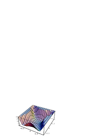
Figure 1: Rescaled potential ${\cal V}(x,y)$

Since the minimization of the F-term potential basically consists of balancing terms that scale like $m_{\pm}^{2}|\phi^{\pm}|^{2}$, $m_{3/2}^{2}|\phi^{\pm}|^{2}$ or with inverse powers of $M_{\rm Pl}$, with the negative term $m_{3/2}^{2}M_{\rm Pl}^{2}$, it is intuitively clear that $x$ and $y$ will be roughly bounded through the most dangerous term by $m_{3/2}m^{-1}_{\pm}$ or ${\cal O}(1)$. This is of course only valid as long as $|\phi^{\pm}|^{2}\gg\xi_{X}$, otherwise $|\phi^{-}|^{2}$ gets tied to $\xi_{X}$. In any case one has that $F_{\phi^{\pm}}/M_{\rm Pl}\lesssim m_{3/2}$, which is sufficient for light gauginos.

2.4 Limiting cases: $m_{3/2}=0$ or $m_{\pm}=0$

We consider now some limiting cases for the above. To see how the model of [6] emerges, we take the flat limit by setting

$$m_{3/2}~{}=~{}0\ .$$ (31)

The two minimization conditions reduce to equations homogeneous in $x,y$ respectively. One can convince oneself that $x=0$ is stable. The solution then reduces to the known case of global supersymmetry, where

$$x~{}=~{}0\ ,\quad y^{2}~{}=~{}\xi_{X}+1\pm\sqrt{1+\frac{2m_{\pm}^{2}}{g_{X}^{2}M_{\rm Pl}^{2}}}~{}\sim~{}\xi_{X}-\frac{m_{\pm}^{2}}{g_{X}^{2}M_{\rm Pl}^{2}}\ .$$ (32)

The auxiliary fields are also identical to (6), since $D_{I}W=\partial_{I}W$. Thus, in this limit, all masses are of the order of $m_{\pm}\sim m$.

On the other hand, it is interesting to study the supergravity corrections to the case that allowed to restore supersymmetry in global supersymmetry, when the mass term in the superpotential is absent,

$$m_{\pm}~{}=~{}0\ .$$ (33)

In this case the solution is given by

$$x^{2}+y^{2}~{}=~{}2-\frac{{\cal V}_{\rm hid}}{m_{3/2}^{2}M_{\rm Pl}^{2}}\ ,\quad x^{2}-y^{2}~{}=~{}-\xi_{X}\ .$$ (34)

Obviously, there is no supersymmetry breaking by D-terms, and $\langle D_{X}\rangle=0$. Actually, in this limit the vacuum energy cannot be fine tuned without extra contributions to the potential, irrespective of ${\cal V}_{\rm hid}$, since it is always given by $-m_{3/2}^{2}M_{\rm Pl}^{2}$. This is however an artifact of the limit $m_{\pm}=0$, and for non-vanishing $m_{\pm}$, the value at the minimum can be shifted by varying ${\cal V}_{\rm hid}$. Finally as a special case of Eq.(34), one may consider the case

$${\cal V}_{\rm hid}~{}=~{}(2-\xi_{X})m_{3/2}^{2}M_{\rm Pl}^{2}$$ (35)

which gives

$$x~{}=~{}0\ ,\quad y^{2}~{}=~{}\xi_{X}\ .$$ (36)

The values of Eq.(36) give the minimum of the potential that is in some sense analogous to the case Eq.(32).

2.5 Multiple $U(1)$ gauge symmetries

With multiple FI-terms in the potential, it is clear that supersymmetry breaking can occur more generically. We have seen above, that FI-terms that cannot be canceled by scalar condensates lead to large scale masses, whereas a scalar condensate with a single FI-term was able to lower the masses to the electro-weak scale $m_{3/2}$, similar to [6]. If multiple FI-terms now come accompanied by the same number of extra charged fields to develop condensates, then the Lagrangian would just be a sum of identical copies of the one of the previous sections, and nothing new is found. An interesting case arises, when there is a mismatch, and not all the FI-parameters can be absorbed by fields like $\phi^{-}$, and thus some large masses can be generated. We now analyze the situation, when there still is only a single set of extra charged fields $\phi^{\pm}$, that takes a non-vanishing expectation value, but there are multiple $U(1)_{a}$ gauge symmetries, under which it is charged. The potential is only modified by summing over D-terms,

$$\kappa^{4}{\cal V}_{D} = \sum_{a}\frac{g_{a}^{2}}{2}\Big{[}\alpha_{a}{\cal K}_{+}|x|^{2}-\alpha_{a}{\cal K}_{-}|y|^{2}+\xi_{a}\Big{]}^{2}\ ,$$

again making $\xi_{a}$ dimensionless by $\xi_{a}\rightarrow\kappa^{-2}\xi_{a}$. Regarding the vacuum energy cancellation, the new minimization conditions read

$${\cal K}_{+}x\Big{[}\kappa^{2}\sum_{a}\alpha_{a}g_{a}^{2}D_{a}+\kappa^{4}{\cal V}_{F}\Big{]}+\frac{m_{\pm}^{2}}{M_{\rm Pl}^{2}}[x+xy^{2}({\cal K}_{+}+{\cal K}_{-})]$$ (37)

$$\hskip 85.35826pt+\frac{m_{3/2}^{2}}{M_{\rm Pl}^{2}}{\cal K}_{+}^{2}x+\frac{m_{\pm}m_{3/2}}{M_{\rm Pl}^{2}}y[({\cal K}_{+}x)^{2}+({\cal K}_{-}y)^{2}+2{\cal K}_{-}-3]~{}=~{}0\ ,$$

$${\cal K}_{-}y\Big{[}-\kappa^{2}\sum_{a}\alpha_{a}g_{a}^{2}D_{a}+\kappa^{4}{\cal V}_{F}\Big{]}+\frac{m_{\pm}^{2}}{M_{\rm Pl}^{2}}[y+x^{2}y({\cal K}_{+}+{\cal K}_{-})]$$

$$\hskip 85.35826pt+\frac{m_{3/2}^{2}}{M_{\rm Pl}^{2}}{\cal K}_{-}^{2}y+\frac{m_{\pm}m_{3/2}}{M_{\rm Pl}^{2}}x[({\cal K}_{+}x)^{2}+({\cal K}_{-}y)^{2}+2{\cal K}_{+}-3]~{}=~{}0\ .$$

It is not necessary to study the general solution here, since the multiple FI-terms already break supersymmetry without the superpotential (3), and one can therefore set $m_{\pm}=0$. With ${\cal K}_{+}={\cal K}_{-}=1$ one can easily solve for $x,y$, finding

$$x^{2}+y^{2}~{}=~{}2-\frac{{\cal V}_{\rm hid}}{m_{3/2}^{2}M_{\rm Pl}^{2}}\ ,\quad x^{2}-y^{2}~{}=~{}-\frac{\sum_{a}g_{a}^{2}\xi_{a}}{M_{\rm Pl}^{2}\sum_{a}g_{a}^{2}}\ .$$ (38)

Thus, in a generic situation, where not all $\xi_{a}$ are equal, supersymmetry will be broken, and $\langle D_{a}\rangle\sim\xi_{a}\sim m_{3/2}M_{\rm Pl}$. In this case, the vacuum energy is given by the negative F-term contribution plus D-terms, and can be fine tuned even without ${\cal V}_{\rm hid}$. The F-terms are given by $F_{\phi^{\pm}}=\kappa^{2}\phi^{\pm}W_{0}\lesssim m_{3/2}M_{\rm Pl}$. The contributions to the scalar masses now look like (with dimensionful $\xi_{a}$)

$$m_{i}^{2}~{}=~{}m_{{\rm gr},i}^{2}+\sum_{a}g_{a}^{2}Q_{a}^{i}D_{a}~{}\sim~{}\sum_{a}g_{a}^{2}Q_{a}^{i}\xi_{a}+\,\cdots$$ (39)

where the terms in parentheses can be of the same order of magnitude, but the gravity-mediated contributions are negligible. This realizes the split supersymmetry scenario, if $\xi_{a}\sim 10^{10-13}\,{\rm GeV}$, for at least two FI-parameters, but with a low gravitino mass $m_{3/2}\sim{\cal O}({\rm TeV})$.

It may also be interesting to note that at the same time all other soft breaking parameters will get modified in the presence of FI-terms and scalar field condensates. This happens through the prefactor $e^{\kappa^{2}{\cal K}}$ in the total potential. For instance, the bi-linear couplings $B$ and the tri-linear couplings $A$ are (see e.g. [18])

$$A_{\alpha\beta\gamma}^{0}\ ,~{}~{}B_{\alpha\beta}^{0}~{}\propto~{}m_{3/2}e^{\kappa^{2}{\cal K}/2}~{}=~{}m_{3/2}(S+\bar{S})^{1/2}e^{\frac{1}{2}(|x|^{2}+|y|^{2})+\,\cdots}\ ,$$ (40)

which may lead to extra suppression factors, depending on the model. Further, we note that the Higgs mixing parameter $\mu$ that enters in the superpotential in the form $\mu H_{1}H_{2}$, where $H_{1}$ and $H_{2}$ are the two Higgs doublets of MSSM, remains essentially unaffected. This is so because in string/supergravity scenarios one expects the $\mu$ term to arise from the Kähler potential using a Kähler tranformation after the spontaneous breaking of supersymmetry has taken place. The Kähler transformation is sensitive to the F-term breaking and not the D-term. Thus, one expects the same mechanism that produces a $\mu$ term of electro-weak size for supergravity models to hold in this case as well.

2.6 Scenarios with partial mass hierarchies

To summarize, there are several scenarios that are possible, which would lead to different patterns in the mass spectrum: $(i)$ There is only one FI-term, and an extra scalar field $\phi^{-}$ beyond the MSSM fields which forms a vacuum expectation value. Here all the soft scalar masses will be of electro-weak size. $(ii)$ In the case of two or more $U(1)_{a}$ with non-vanishing $\xi_{a}$, and the charges $Q^{i}_{a}$ non-zero and sufficiently generic, the scalar masses are of the order of $\xi_{a}$, while the gauginos stay light. One can thus get a hierarchical splitting of scalar and fermion masses. $(iii)$ One may also achieve hybrid scenarios, when only some of the charges $Q_{a}^{i}$ are non-vanishing, or such that the high mass terms just cancel out. Below we consider two specific scenarios with partial splitting of scalars. The implications of this partially split scenario will be very different from the usual SUGRA scenario and also from the high scale supersymmetry scenario of split supersymmetry.

2.6.1 Model I: $2+1$ generations

As the first model we consider the case with non-vanishing charges for the first and second generation of squarks and sleptons, but vanishing charges for the third generation. In this circumstance the former will develop super heavy masses and will not be accessible at the LHC, as opposed to the third generation. The above implies that the dangerous flavor changing neutral currents will be automatically suppressed. Some of the signals of this scenario will be very unique, such as the decay of the gluino ($\tilde{g}$). In SUGRA its decay modes are as follows

$$\tilde{g}~{}\rightarrow~{}\bar{u}_{i}\tilde{u}_{i}\,,\ \bar{d}_{i}\tilde{d}_{i}~{}\rightarrow~{}\left\{{u_{i}\bar{u}_{i}\tilde{\chi}_{j}^{0}\,,\ d_{i}\bar{d}_{i}\tilde{\chi}_{j}^{0}\atop u_{i}\bar{d}_{i}\tilde{\chi}_{k}^{-}\,,\ d_{i}\bar{u}_{i}\tilde{\chi}_{k}^{+}}\right.\ .$$ (41)

where $i=1,2,3$ are the generational indices, $j=1,2,3,4$, and $k=1,2$ for neutralinos and charginos. However, for the case of the model under consideration the decay through the first two generations is highly suppressed, and the gluino decay can only occur through third generation squarks via the modes $\tilde{g}\rightarrow b\bar{b}\tilde{\chi}_{j}^{0}$ with admixtures of $\tilde{g}\rightarrow b\bar{t}\tilde{\chi}_{k}^{+}$, $\tilde{g}\rightarrow t\bar{b}\tilde{\chi}_{k}^{-}$, and $\tilde{g}\rightarrow t\bar{t}\tilde{\chi}_{j}^{0}$, depending on the gluino mass. There will be no contribution to the anomalous magnetic moment of the muon at the one-loop level. The following set of phases can arise: $\theta_{\mu}$, $\xi_{i}$, and $\alpha_{A}$, where $\theta_{\mu}$ is the phase of the Higgs mixing parameter $\mu$, $\xi_{i}$ ($i=1,2,3$) are the phases of the $SU(3)_{c}$, $SU(2)_{L}$ and $U(1)_{Y}$ gaugino masses, and $\alpha_{A}$ is the phase of the common trilinear coupling for the third generation scalars (However, it should be kept in mind that not all the phases are independent and only certain combinations enter in physical processes). Because of the super heavy nature of the first two generations, the one-loop contributions to the electric dipole mement (edm) of the electron and of the neutron are highly suppressed. However, there can be higher loop corrections to the edms. Specifically, the neutron edm can get a contribution from the CP violating dimension six operator. Unification of gauge coupling constants at the one-loop level will remain unchanged, although at the two-loop level there will be effects from the splittings. In this model the staus can be light and thus co-annihilation of the LSP neutralinos with the staus can occur, allowing for the possibility that the neutralino relic density could be consistent with the current data. Finally, proton decay from dimension five operators would not arise via dressings from the first and second generation squarks and sleptons, but can arise from the dressings of the third generation sfermions.

2.6.2 Model II: ${\bf 5}+{\bf 10}$ split spectrum

As another illustrative example, we consider a model where the squarks and sleptons belonging to a 10 of $SU(5)$ have non-vanishing charges and high scale masses, while the squarks and sleptons belonging to a 5 have vanishing charges. In this case, the only light scalars aside from Higgs bosons will be $\tilde{d}^{C}_{i},\tilde{e}_{Li},\tilde{\nu}_{i}$ ($i=1,2,3$). In this model, unlike the case of model I, there is a one-loop supersymmetric contribution to the muon anomalous magnetic moment $g_{\mu}-2$. The CP phases in this model consist of $\theta_{\mu}$ and $\xi_{i}$ ($i=1,2,3$). There also is a one-loop supersymmetric contribution to the edms of the electron and of the neutron. Further, the decays of the gluino, the chargino and the neutralino can occur only via a smaller subset of states and thus their decay widths will be relatively smaller, though they will still decay within the detection chamber. Finally proton decay through dimension five operators will be highly suppressed in this model and the dominant decay will occur through the usual vector boson interactions.

3 Hierarchical Breaking in D-brane models

We turn now to the question of how the models discussed so far fit into string theory, in particular in the class of intersecting or magnetized D-brane models [19, 20]. These are models within orientifold string compactifications of type II strings with D-branes that wrap parts of the internal compactification space, and either with magnetic field backgrounds on the brane world volume (in type IIB) or with the branes intersecting non-trivially on the internal space (in type IIA) [21]. For these models a great deal about the Lagrangian of their low energy field theory description is known, e.g. in [22, 23], and the soft supersymmetry breaking terms in the conventional setting with F-terms generated in the hidden sector, have been determined. Furthermore, it is known how FI-terms can appear [24].

The gauge group for any single stack of $N_{a}$ D-branes is $U(N_{a})=SU(N_{a})\times U(1)_{a}$ (only sometimes an $Sp(N_{a})$ or $SO(2N_{a})$ subgroup thereof), and thus involves extra abelian $U(1)_{a}$ factors, when the Standard Model is engineered. In the first models that were constructed to reproduce the non-supersymmetric Standard Model [20], there are four extra $U(1)_{a}$, including the anomaly-free hyper charge and gauged $B-L$ quantum numbers, but also two extra $U(1)$ factors which are anomalous. The relevant anomaly is actually a mixed abelian-non-abelian anomaly, i.e. there are triangle diagrams of the type $SU(N_{b})^{2}-U(1)_{a}$ non-vanishing for either $SU(2)$ or $SU(3)$. In particular, ${\rm tr}(Q_{a})=0$, and there is no gravitational anomaly. While the first models were non-supersymmetric from the beginning, the structure of charge assignments, given in table 1 of [20], and the number of $U(1)_{a}$ can serve as a representative example. From this it is clear that these models at least contain two candidate $U(1)_{a}$, which may develop FI-terms. In generality, it is known that, when D-branes violate supersymmetry, this is reflected by FI-terms in the effective theory [24]. The violation of supersymmetry translates into a violation of the $\kappa$-symmetry on their world volume, and is geometrically captured by a violation of the so-called calibration conditions. For intersecting D-branes models, this has a very simple geometric interpretation. Any single brane wraps a three-dimensional internal space. In the case of an orbifold compactification it is characterized by three angles $\varphi_{i}^{a}$, $i=1,2,3$, one for each $\mathbb{T}^{2}$ in $\mathbb{T}^{6}=(\mathbb{T}^{2})^{3}$, measuring the relative angle of the D-brane with respect to some reference orientifold plane. The supersymmetry condition reads $\varphi_{1}^{a}\pm\varphi_{2}^{a}\pm\varphi_{3}^{a}=0\,{\rm mod}\,2\pi$, with some choice of signs. The FI-parameter at leading order is proportional to the deviation,

$$\alpha^{\prime}\xi_{a}~{}\sim~{}\varphi_{1}^{a}\pm\varphi_{2}^{a}\pm\varphi_{3}^{a}\ {\rm mod}\ 2\pi\ .$$ (42)

The angles are moduli-dependent quantities, and thus the question if a FI-term is generated cannot be finally answered without solving the moduli stabilization problem for the relevant moduli. In the mirror symmetric type IIB description with magnetized branes this is manifest, and the relation reads

$$\alpha^{\prime}\xi_{a}~{}\sim~{}\frac{f_{a}^{1}}{T_{1}+\bar{T}_{\bar{1}}}\pm\frac{f_{a}^{2}}{T_{2}+\bar{T}_{\bar{2}}}\pm\frac{f_{a}^{3}}{T_{3}+\bar{T}_{\bar{3}}}\ ,$$ (43)

where $f_{a}^{i}/(T_{i}+\bar{T}_{\bar{\imath}})=\tan(\varphi_{i}^{a})$, and the $T_{i}$ are the three (dimensionless) moduli, whose real parts measure the sizes of the three $\mathbb{T}^{2}$, while the $f_{a}^{i}$ are rational numbers. The natural scale for the FI-parameter is the string scale $M_{s}=(\alpha^{\prime})^{-1/2}$, and a suppression means that the right-hand-side is small numerically.

Another very important property of the string theoretic embedding of D-terms is the fact that tachyonic masses (negative mass squared) can be lifted to positive values. Inspecting the charge assignments e.g. in [20], one realizes that it is not feasible to have positive charges under the $U(1)_{a}$ for all the fields of the MSSM. This would naively mean that some $m_{i}^{2}\sim g_{a}^{2}Q_{a}^{i}D_{a}$ are negative, which would lead to a breakdown of gauge symmetry. However, in the particular case of orbifold models, the exact string quantization can be performed, and the mass spectrum computed for small FI-parameters, without using effective field theory. It turns out that for small angles ($\varphi_{i}^{ab}=\varphi_{i}^{a}-\varphi_{i}^{b}<\pi/2$), the mass of the lowest excitation of two intersecting branes $a$ and $b$ is given by

$$\alpha^{\prime}m_{i}^{2}=\frac{1}{2}\sum_{i=1}^{3}|\varphi_{i}^{ab}|-{{\rm max}_{i}}\{|\varphi_{i}^{ab}|\}\ ,$$ (44)

which, for a proper choice of signs, vanishes precisely if $\xi_{a}=0$, consistent with the effective description. However, depending on the angles, there is a region in parameter space, where the deviation from $\xi_{a}=0$ only induces positive squared masses, and no tachyons (see e.g. [26] in this context). This comes as a surprise from the low energy point of view, and is explained by the presence of higher order corrections in the derivative expansion of the Born-Infeld effective action, which become important for strings stretching between intersecting branes [27]. The conclusion is, that the effective mass that follows from the D-term potential is corrected to positive values, and we can tolerate tachyons in the field theoretic models.

Taking these observations together, it seems first of all possible that D-brane models of the type discussed have mass spectra with important contributions from FI-terms. Since multiple extra $U(1)_{a}$ factors exist and turn anomalous, a scenario, where the $D_{a}$ fields cannot be relaxed to the electro-weak scale, appears plausible. This would imply a mass hierarchy between charged scalars and fermions. To solve the moduli stabilization problem, and show convincingly how the D- and F-terms of the desired magnitude are generated dynamically, of course, remains an open challenge. One may also want to turn the argument around, to conclude that within the conventional approach with low energy supersymmetry, the potential presence of many FI-terms is a great danger for these types of models, and one has to find ways to suppress them dynamically.

Finally, we like to mention a caveat which makes the classes of D-branes models that we discussed rather not so good candidates to realize split supersymmetry. It is well known that in D-brane models in general the unification of gauge interactions really only happens at the string scale, and not in the field theory regime. This means that the original motivation to keep the gauginos and higgsinos light, while giving up on the scalars, is upset. The gauge kinetic functions are moduli-dependent $f_{a}=f_{a}(T_{I})$, and a unification of couplings requires some relations among moduli to hold [28, 23, 25], which so far can appear accidentally in various models in the literature, but do not seem to have any independent justification. This means, that an essential motivation for split supersymmetry, gauge unification, is only accidentally realized.

4 Hierarchical D-term inflation

In hierarchical supersymmetry breaking of the type discussed here it seems an intriguing suggestion to relate the mass scale of the heavy scalars to cosmology. In our model, the potential energy is generated at the conventional supersymmetry breaking scale $(m_{3/2}M_{\rm Pl})^{2}$, and with standard values comes out about $(10^{10-13}\,{\rm GeV})^{4}$. This is the scale of the individual contributions of the F- and D-terms to the full potential, and only the fine tuning of the cosmological constant leads to a cancellation. It is now very tempting to identify the vacuum energy of these individual components with the vacuum energy that drives inflation, by undoing the fine tuning. A possible scenario is very easily illustrated along the lines of D-term inflation [29]. Roughly speaking, the only required modification of the model we used so far, with the MSSM extended by one or many extra $U(1)_{a}$ gauge factors, plus a pair of charged fields $\phi^{\pm}$, is to promote the mass term (3) in the superspotential to a dynamical field $\varphi$, neutral under $U(1)_{a}$, which plays the role of the inflaton. We now write

$$W~{}=~{}\varphi\phi^{+}\phi^{-}+W_{0}\ ,$$ (45)

and use a canonically normalized Kähler potential,

$${\cal K}~{}=~{}|\phi^{+}|^{2}+|\phi^{-}|^{2}+|\varphi|^{2}+{\cal K}_{0}\ .$$ (46)

With this one finds the scalar potential of the form

$${\cal V} = {\cal V}_{\rm hid}+e^{\kappa^{2}{\cal K}}\Big{[}|\varphi\phi^{+}|^{2}+|\varphi\phi^{-}|^{2}+|\phi^{+}\phi^{-}|^{2}+\kappa^{4}\big{(}|\varphi|^{2}+|\phi^{+}|^{2}+|\phi^{-}|^{2}\big{)}|W|^{2}$$ (47)

$$\hskip 28.45274pt+3\kappa^{2}|\varphi\phi^{+}\phi^{-}|^{2}-3\kappa^{2}|W_{0}|^{2}\Big{]}+\sum_{a}\frac{g_{a}^{2}}{2}\Big{[}|\phi^{+}|^{2}-|\phi^{-}|^{2}+\xi_{a}\Big{]}^{2}\ ,$$

where the only negative contribution comes from $-3\kappa^{2}e^{\kappa^{2}{\cal K}}|W_{0}|^{2}$. Above some threshold value for $\varphi$, the two charged fields $\phi^{\pm}$ are stabilized at the origin $\phi^{\pm}=0$. Their masses at zero are

$$m^{2}_{\phi^{\pm}}(\phi^{\pm}=0)~{}=~{}\kappa^{2}{\cal V}_{\rm hid}+e^{\kappa^{2}{\cal K}_{0}}[(1+\kappa^{6}|W_{0}|^{2})|\varphi|^{2}-2\kappa^{4}|W_{0}|^{2}]\pm\sum_{a}g_{a}^{2}\xi_{a}\ ,$$ (48)

which turns positive, when $\langle\varphi\rangle$ is large enough (but still well below the Planck scale). The potential simplifies to

$${\cal V}(\phi^{\pm}=0)~{}=~{}{\cal V}_{\rm hid}+\kappa^{2}e^{\kappa^{2}{\cal K}_{0}}|W_{0}|^{2}[\kappa^{2}|\varphi|^{2}-3]+\sum_{a}\frac{g_{a}^{2}}{2}\xi_{a}^{2}\ .$$ (49)

The inflationary slow-roll condition for the second derivative of the potential is [30]

$$|\eta|~{}=~{}\left|\frac{\partial_{\varphi}^{2}{\cal V}}{\kappa^{2}{\cal V}}\right|~{}\ll~{}1\ ,$$ (50)

where $|\eta|\ll 1$ numerically means $|\eta|\sim 0.01$ is acceptable. This implies that

$$\frac{M_{\rm Pl}^{2}\sum_{a}g_{a}^{2}\xi_{a}^{2}}{e^{\kappa^{2}{\cal K}}|W_{0}|^{2}}~{}\gtrsim~{}100\ .$$ (51)

The first derivative is then automatically also small (with $\varphi\sim\sqrt{\xi_{a}}$), and inflation can be successful. This means that the very same D-term vacuum energy that is responsible for the large scalar masses can drive inflation, if either the D-terms are enhanced or the F-term vacuum energy is sufficiently suppressed during that period. Thus, during the de Sitter phase the relation between the Hubble parameter $H$ and the energy density $\rho$, i.e. the relation $3M_{\rm Pl}^{2}H^{2}=\rho=\frac{1}{2}\dot{\phi}^{2}+{\cal V}$, shows that the Hubble expansion in this phase is dominated by the FI-term

$$3M_{\rm Pl}^{2}H^{2}~{}\sim~{}\sum_{a}\frac{g_{a}^{2}}{2}\xi^{2}_{a}\ .$$ (52)

In summary, if in the phase of large $\varphi$ the vacuum energy of the D-terms is larger than that of the F-terms by a factor of about 100 or more, the D-term energy can drive inflation at a scale up to $10^{12-15}\,{\rm GeV}$, slightly above the mass scale of the heavy scalars. After the end of the slow roll period, $\varphi$ will eventually fall below the threshold value, and $\phi^{\pm}$ will form condensates themselves. This can then lead to a partial relaxation of the D-term vacuum energy, but a more elaborate model of the hidden sector would be needed to describe this phase transition properly. In the minimum, one may expect $\varphi$ to settle down to $\langle\varphi\rangle\sim\sqrt{\xi}\sim\sqrt{m_{3/2}M_{\rm Pl}}$ on dimensional grounds, which is compatible with small gaugino masses.

5 Conclusion

We have presented a model of supersymmetry breaking in the context of string and supergravity scenarios by inclusion of both F- and Fayet-Iliopoulos D-terms, arising from extra $U(1)$ factors in the gauge group. Such extra $U(1)$ gauge symmetries arise quite naturally in string based models. It was shown that scalars charged under the extra $U(1)$ gain large masses from the FI-terms, proportional to the charges of the respective scalar fields under the extra $U(1)$. This leads generically to non-universal masses for the heavy scalars. The cancellation of the vacuum energy puts an upper bound of $\sqrt{m_{3/2}M_{\rm Pl}}$ on the scalar masses, and thus also puts a bound on the FI-term $\xi_{X}$. The bound on $\xi_{X}$ can be met in heterotic string models only for $m_{3/2}$ close to $M_{\rm Pl}$, since there $\xi_{X}$ is scaled by $M_{\rm Pl}^{2}$. Thus, heterotic string scenarios are not preferred from the vacuum energy constraint, when $m_{3/2}={\cal O}({\rm TeV})$. However, $m_{3/2}={\cal O}({\rm TeV})$ and $\xi_{X}\sim m_{3/2}M_{\rm Pl}$, i.e. of size $10^{10-13}\,{\rm GeV}$, could arise in orientifolds models which allow $\xi_{X}$ of a variable moduli-dependent size. The fact that the D-term contributions to the scalar masses depend on their $U(1)$ charges opens up the possibility of building a new class of models with some scalars (with vanishing $U(1)$ charges) light and others (with non-vanishing $U(1)$ charges) heavy, while the gauginos and higgsinos gain masses only of electro-weak size. Further, the $\mu$ term is essentially unaffected by the FI contribution, and can be of electro-weak size. We investigated two illustrative examples of models with light and heavy scalars (Model I and Model II in Sec. 2) and showed that they lead to significantly different phenomenologies which could be tested at colliders and in non-accelerator experiment. The class of models we have discussed here are different from the high scale supersymmetry models of Ref. [2], where all scalars and the gravitino are super heavy. However, which scalars are heavy and which are light is now a model-dependent question. A further interesting feature is the possibility that the vacuum energy responsible for generating heavy scalars may also drive inflation. An analysis of how this can come about was discussed in Sec. 4. It would be interesting to investigate more explicit D-brane constructions to build models of the type advocated here.

References

- [1] A. H. Chamseddine, R. Arnowitt and P. Nath, Locally Supersymmetric Grand Unification, Phys. Rev. Lett. 49 (1982) 970; R. Barbieri, S. Ferrara and C. A. Savoy, Gauge Models with Spontaneously Broken Local Supersymmetry, Phys. Lett. B 119 (1982) 343; P. Nath, R. Arnowitt and A. H. Chamseddine, Gauge Hierarchy in Supergravity Guts, Nucl. Phys. B 227 (1983) 121; L. J. Hall, J. Lykken and S. Weinberg, Supergravity as the Messenger of Supersymmetry Breaking, Phys. Rev. D 27 (1983) 2359.
- [2] N. Arkani-Hamed and S. Dimopoulos, Supersymmetric Unification without Low Energy Supersymmetry and Signatures for Fine-tuning at the LHC, hep-th/0405159.
- [3] L. Susskind, The Anthropic Landscape of String Theory, hep-th/0302219; M. R. Douglas, The Statistics of String/M Theory Vacua, JHEP 0305 (2003) 046 [hep-th/0303194]; T. Banks, M. Dine and E. Gorbatov, Is there a String Theory Landscape?, JHEP 0408 (2004) 058 [hep-th/0309170].
- [4] G. F. Giudice and A. Romanino, Split Supersymmetry, Nucl. Phys. B 699 (2004) 65 [hep-ph/0406088]; N. Arkani-Hamed, S. Dimopoulos, G. F. Giudice and A. Romanino, Aspects of Split Supersymmetry, hep-ph/0409232.
- [5] A. Arvanitaki, C. Davis, P. W. Graham and J. G. Wacker, One Loop Predictions of the Finely Tuned SSM, hep-ph/0406034; A. Pierce, Dark Matter in the Finely Tuned Minimal Supersymmetric Standard Model, Phys. Rev. D 70 (2004) 075006 [hep-ph/0406144]; C. Kokorelis, Standard Models and Split Supersymmetry from Intersecting Brane Orbifolds, hep-th/0406258; S. H. Zhu, Chargino Pair Production at Linear Collider and Split Supersymmetry, hep-ph/0407072; B. Mukhopadhyaya and S. SenGupta, Sparticle Spectrum and Phenomenology in Split Supersymmetry: Some Possibilities, hep-th/0407225; W. Kilian, T. Plehn, P. Richardson and E. Schmidt, Split Supersymmetry at Colliders, hep-ph/0408088; R. Mahbubani, Bounds on the Higgs Mass in Variations of Split Supersymmetry, hep-ph/0408096; M. Binger, The Higgs Boson Mass at 2 Loops in the Finely Tuned Split Supersymmetric Standard Model, hep-ph/0408240; J. L. Hewett, B. Lillie, M. Masip and T. G. Rizzo, Signatures of Long-lived Gluinos in Split Supersymmetry, JHEP 0409 (2004) 070 [hep-ph/0408248]; L. Anchordoqui, H. Goldberg and C. Nunez, Probing Split Supersymmetry with Cosmic Rays, hep-ph/0408284; K. Cheung and W. Y. Keung, Split Supersymmetry, Stable Gluino, and Gluinonium, hep-ph/0408335; D. A. Demir, Effects of Flavor Violation on Split Supersymmetry, hep-ph/0410056. R. Allahverdi, A. Jokinen and A. Mazumdar, Gravitino Production from Reheating in Split Supersymmetry, hep-ph/0410169. V. Barger, C. W. Chiang, J. Jiang and T. Li, Axion Models with High-scale Supersymmetry Breaking, hep-ph/0410252. J. A. Casas, J. R. Espinosa and I. Hidalgo, Implications for New Physics from Fine-tuning Arguments. I: Application to SUSY and Seesaw Cases, hep-ph/0410298. B. Bajc and G. Senjanovic, Radiative Seesaw: A Case for Split Supersymmetry, hep-ph/0411193.
- [6] G. R. Dvali and A. Pomarol, Anomalous U(1) as a Mediator of Supersymmetry Breaking, Phys. Rev. Lett. 77 (1996) 3728 [hep-ph/9607383].
- [7] P. Binetruy and E. Dudas, Gaugino Condensation and the Anomalous U(1), Phys. Lett. B 389 (1996) 503 [hep-th/9607172].
- [8] L. Randall and R. Sundrum, Out of this World Supersymmetry Breaking, Nucl. Phys. B 557 (1999) 79 [hep-th/9810155]; G. F. Giudice, M. A. Luty, H. Murayama and R. Rattazzi, Gaugino Mass without Singlets, JHEP 9812 (1998) 027 [hep-ph/9810442].
- [9] I. Antoniadis and T. R. Taylor, Topological Masses from Broken Supersymmetry, Nucl. Phys. B 695 (2004) 103 [hep-th/0403293].
- [10] M. Klein, Anomaly Cancellation in D = 4, N = 1 Orientifolds and Linear/Chiral Multiplet Duality, Nucl. Phys. B 569 (2000) 362 [hep-th/9910143]; H. Ruegg and M. Ruiz-Altaba, The Stueckelberg Field, Int. J. Mod. Phys. A 19 (2004) 3265 [hep-th/0304245]. B. Körs and P. Nath, A Stueckelberg Extension of the Standard Model, Phys. Lett. B 586 (2004) 366 [hep-ph/0402047]; A Supersymmetric Stueckelberg U(1) Extension of the MSSM, hep-ph/0406167; J. Louis and W. Schulgin, Massive Tensor Multiplets in N = 1 Supersymmetry, hep-th/0410149.
- [11] Z. Lalak, S. Lavignac and H. P. Nilles, String Dualities in the Presence of Anomalous U(1) Symmetries, Nucl. Phys. B 559 (1999) 48 [hep-th/9903160]; H. P. Nilles, Remarks on Anomalous U(1) Symmetries in String Theory, hep-ph/0003102.
- [12] M. Dine, N. Seiberg and E. Witten, Fayet-Iliopoulos Terms in String Theory, Nucl. Phys. B 289 (1987) 589; J. J. Atick, L. J. Dixon and A. Sen, String Calculation of Fayet-Iliopoulos D Terms in Arbitrary Supersymmetric Compactifications, Nucl. Phys. B 292 (1987) 109;
- [13] C. Angelantonj and A. Sagnotti, Open Strings, Phys. Rept. 371 (2002) 1 [Erratum-ibid. 376 (2003) 339] [hep-th/0204089].
- [14] L. E. Ibanez, R. Rabadan and A. M. Uranga, Anomalous U(1)’s in Type I and Type IIB D = 4, N = 1 String Vacua, Nucl. Phys. B 542 (1999) 112 [hep-th/9808139].
- [15] E. Poppitz, On the One Loop Fayet-Iliopoulos Term in Chiral Four Dimensional Type I Orbifolds, Nucl. Phys. B 542 (1999) 31 [hep-th/9810010].
- [16] A. Chamseddine, R. Arnowitt and P. Nath in [1]; E. Cremmer, S. Ferrara, L. Girardello and A. Van Proeyen, Yang-Mills Theories with Local Supersymmetry: Lagrangian, Transformation Laws and Superhiggs Effect, Nucl. Phys. B 212 (1983) 413.
- [17] V. S. Kaplunovsky and J. Louis, Model Independent Analysis of Soft Terms in Effective Supergravity and in String Theory, Phys. Lett. B 306 (1993) 269 [hep-th/9303040].
- [18] P. Nath and T. R. Taylor, Modular Invariance, Soft Breaking, mu and tan(beta) in Superstring Models, Phys. Lett. B 548 (2002) 77 [hep-ph/0209282].
- [19] R. Blumenhagen, L. Görlich, B. Körs and D. Lüst, Noncommutative Compactifications of Type I Strings on Tori with Magnetic Background Flux, JHEP 0010 (2000) 006 [hep-th/0007024]; C. Angelantonj, I. Antoniadis, E. Dudas and A. Sagnotti, Type-I Strings on Magnetised Orbifolds and Brane Transmutation, Phys. Lett. B 489 (2000) 223 [hep-th/0007090]; G. Aldazabal, S. Franco, L. E. Ibanez, R. Rabadan and A. M. Uranga, D = 4 Chiral String Compactifications from Intersecting Branes, J. Math. Phys. 42 (2001) 3103 [hep-th/0011073]; M. Cvetic, G. Shiu and A. M. Uranga, Chiral Four-dimensional N = 1 Supersymmetric Type IIA Orientifolds from Intersecting D6-branes, Nucl. Phys. B 615 (2001) 3 [hep-th/0107166].
- [20] L. E. Ibanez, F. Marchesano and R. Rabadan, Getting Just the Standard Model at Intersecting Branes, JHEP 0111 (2001) 002 [hep-th/0105155].
- [21] C. Bachas, A Way to Break supersymmetry, hep-th/9503030; M. Berkooz, M. R. Douglas and R. G. Leigh, Branes Intersecting at Angles, Nucl. Phys. B 480 (1996) 265 [hep-th/9606139].
- [22] D. Cremades, L. E. Ibanez and F. Marchesano, SUSY Quivers, Intersecting Branes and the Modest Hierarchy Problem, JHEP 0207 (2002) 009 [hep-th/0201205]; M. Cvetic and I. Papadimitriou, Conformal Field Theory Couplings for Intersecting D-branes on Orientifolds, Phys. Rev. D 68(2003) 046001 [Erratum-ibid. D 70 (2004) 029903] [hep-th/0303083]; S. A. Abel and A. W. Owen, Interactions in Intersecting Brane Models, Nucl. Phys. B 663 (2003) 197 [hep-th/0303124]; P. G. Camara, L. E. Ibanez and A. M. Uranga, Flux-induced SUSY-breaking Soft Terms, Nucl. Phys. B 689 (2004) 195 [hep-th/0311241]; Flux-induced SUSY-breaking Soft Terms on D7-D3 Brane Systems, hep-th/0408036; D. Lüst, P. Mayr, R. Richter and S. Stieberger, Scattering of Gauge, Matter, and Moduli Fields from Intersecting Branes, Nucl. Phys. B 696 (2004) 205 [hep-th/0404134]; D. Lüst, S. Reffert and S. Stieberger, Flux-induced Soft Supersymmetry Breaking in Chiral Type IIb Orientifolds with D3/D7-branes, hep-th/0406092; MSSM with Soft SUSY Breaking Terms from D7-branes with Fluxes, hep-th/0410074.
- [23] B. Körs and P. Nath, Effective Action and Soft Supersymmetry Breaking for Intersecting D-brane Models, Nucl. Phys. B 681 (2004) 77 [hep-th/0309167].
- [24] M. R. Douglas and G. W. Moore, D-branes, Quivers, and ALE Instantons, hep-th/9603167; D. Cremades, L. E. Ibanez and F. Marchesano, Intersecting Brane Models of Particle Physics and the Higgs Mechanism, JHEP 0207 (2002) 022 [hep-th/0203160]; R. Blumenhagen, V. Braun, B. Körs and D. Lüst, Orientifolds of K3 and Calabi-Yau Manifolds with Intersecting D-branes, JHEP 0207 (2002) 026 [hep-th/0206038].
- [25] I. Antoniadis and S. Dimopoulos, Splitting Supersymmetry in String Theory, hep-th/0411032.
- [26] R. Rabadan, Branes at Angles, Torons, Stability and Supersymmetry, Nucl. Phys. B 620 (2002) 152 [hep-th/0107036].
- [27] A. Hashimoto and W. I. Taylor, Fluctuation Spectra of Tilted and Intersecting D-branes from the Born-Infeld Action, Nucl. Phys. B 503 (1997) 193 [hep-th/9703217]; F. Denef, A. Sevrin and J. Troost, Non-Abelian Born-Infeld versus String Theory, Nucl. Phys. B 581 (2000) 135 [hep-th/0002180].
- [28] R. Blumenhagen, D. Lüst and S. Stieberger, Gauge Unification in Supersymmetric Intersecting Brane Worlds, JHEP 0307 (2003) 036 [hep-th/0305146].
- [29] P. Binetruy and G. R. Dvali, D-term Inflation, Phys. Lett. B 388 (1996) 241 [hep-ph/9606342]; E. Halyo, Hybrid Inflation from Supergravity D-terms, Phys. Lett. B 387 (1996) 43 [hep-ph/9606423]; P. Binetruy, G. Dvali, R. Kallosh and A. Van Proeyen, Fayet-Iliopoulos Terms in Supergravity and Cosmology, Class. Quant. Grav. 21 (2004) 3137 [hep-th/0402046].
- [30] A. R. Liddle and D. H. Lyth, Cosmological Inflation and Large Scale Structure, Cambridge University Press, 2000.
- [31] S. Kachru, R. Kallosh, A. Linde, J. Maldacena, L. McAllister and S. P. Trivedi, Towards Inflation in String Theory, JCAP 0310 (2003) 013 [hep-th/0308055]; J. P. Hsu, R. Kallosh and S. Prokushkin, On Brane Inflation with Volume Stabilization, JCAP 0312 (2003) 009 [hep-th/0311077]; H. Firouzjahi and S. H. H. Tye, Closer Towards Inflation in String Theory, Phys. Lett. B 584 (2004) 147 [hep-th/0312020]; M. Berg, M. Haack and B. Körs, Loop Corrections to Volume Moduli and Inflation in String Theory, hep-th/0404087; On the Moduli Dependence of Nonperturbative Superpotentials in Brane Inflation, hep-th/0409282; H. Jockers and J. Louis, The Effective Action of D7-branes in N = 1 Calabi-Yau Orientifolds, hep-th/0409098.
- [32] S. Kachru, R. Kallosh, A. Linde and S. P. Trivedi, De Sitter Vacua in String Theory, Phys. Rev. D 68 (2003) 046005 [hep-th/0301240].