Phantom Friedmann Cosmologies and Higher-Order Characteristics of Expansion

Abstract

We discuss a more general class of phantom ($p<-\varrho$) cosmologies with various forms of both phantom ($w<-1$), and standard ($w>-1$) matter. We show that many types of evolution which include both Big-Bang and Big-Rip singularities are admitted and give explicit examples. Among some interesting models, there exist non-singular oscillating (or ”bounce”) cosmologies, which appear due to a competition between positive and negative pressure of variety of matter content. From the point of view of the current observations the most interesting cosmologies are the ones which start with a Big-Bang and terminate at a Big-Rip. A related consequence of having a possibility of two types of singularities is that there exists an unstable static universe approached by the two asymptotic models - one of them reaches Big-Bang, and another reaches Big-Rip. We also give explicit relations between density parameters $\Omega$ and the dynamical characteristics for these generalized phantom models, including higher-order observational characteristics such as jerk and ”kerk”. Finally, we discuss the observational quantities such as luminosity distance, angular diameter, and source counts, both in series expansion and explicitly, for phantom models. Our series expansion formulas for the luminosity distance and the apparent magnitude go as far as to the fourth-order in redshift $z$ term, which includes explicitly not only the jerk, but also the ”kerk” (or ”snap”) which may serve as an indicator of the curvature of the universe.

I Introduction

Phantom is matter which possesses a very strong negative pressure and so it violates the null energy condition $\varrho+p>0$, where $\varrho$ is the energy density and $p$ is the pressure. Consequently it violates all the remained energy conditions: the strong, the weak and the dominant. In terms of the barotropic equation of state $p=w\varrho$ ($w=$ const.) phantom is described as matter with $w<-1$. The story of phantom and its observational support is not quite analogous to the story of quintessence or dark energy - the matter which violates the strong energy condition $\varrho+3p>0$, i.e., the matter which allows $w<-1/3$. Namely, despite its theoretical investigations striwall ; AJIII , and even admission for the early universe inflation, it was hardly accepted as reality before the first supernovae data was revealed perlmutter . A different story happens with phantom. A more detailed check of the data suggests that the current supernovae not only gives evidence for quintessence with $-1<w<-1/3$, but also admits phantom with $w<-1$ at a high confidence level supernovae . The point is that in view of the data from supernovae there is no sharp cut-off of the admissible values of $w$ at $w=-1$. Instead, the data even favours the values of $w$ which are less than minus one.

Phantom matter was first investigated in the current cosmological context by Caldwell caldwell99 , who also suggested the name referring to its curiosity. In fact, phantom (or ghost) must possess negative energy which leads to instabilities on both classical and quantum level instabilities ; nojiri04 . Since it violates all possible energy conditions, it also puts in doubt the pillars of relativity and cosmology such as: the positive mass theorems, the laws of black hole thermodynamics, the cosmic censorship, and causality in relativity theory he ; visser . In this context phantom becomes a real challenge for the theory, if its support from the the supernovae data is really so firm. The thing is that the main support for the phantom comes from supernovae dimming rather than from large-scale structure and cosmic microwave background observations. That is why some alternative explanation of the dimming of supernovae due to a conversion of cosmological term and photons into axions was made kaloper . From the theoretical point of view - a release of the assumption of an analytic equation of state which relates energy density and pressure and does not lead to energy conditions violation (except for the dominant one) may also be useful barrow04 . As for the explanation of the supernovae data phantom is also useful in killing the doubled positive pressure contribution in braneworld models braneIa .

Phantom type of matter was also implicitly suggested in cosmological models with a particle production john88 , in higher-order theories of gravity models Pollock88 , Brans-Dicke models for $\omega<-\frac{3}{2}$, in non-minimally coupled scalar field theories starob00 , in mirage cosmology of the braneworld scenario kiritsis , and in kinematically-driven quintessence (k-essence) models chiba , for example. The interest in phantom has grown vastly during the last two years and various aspects of phantom models have been investigated Hann02 ; Frampt02 ; Frampt03 ; FramTaka02 ; McInnes ; trodden1 ; trodden2 ; Bastero01 ; Bastero02 ; abdalla04 ; Erickson ; BIphantom ; LiHao03 ; singh03 ; nojiri031 ; nojiri032 ; nojiri033 ; nojiri034 ; simphan ; onemli ; diaz ; zhang ; cai .

One of the most interesting features of phantom models is that they allow for a Big-Rip (BR) curvature singularity, which appears as a result of having the infinite values of the scale factor $a(t)\to\infty$ at a finite future. However, as it was already mentioned, the evidence for phantom from observations is mainly based on the assumption of the barotropic equation of state which tightly constraints the energy density and the pressure. It is puzzling barrow04 that for Friedmann cosmological models which do not admit an equation of state which links the energy density $\varrho$ and the pressure $p$, a sudden future singularity of pressure may appear. This is a singularity of pressure only, with finite energy density which has an interesting analogy with singularities which appear in some inhomogeneous models of the universe dabrowski93 ; dabrowski95 ; inhosfs .

Recently, phantom cosmologies which lead to a quadratic polynomial in canonical Friedmann equation have been investigated phantom1 . However, only the two types of phantom matter with the equations of state $p=-(4/3)\varrho$ (phantom) and $p=-(5/3)\varrho$ (superphantom) were admitted. In this paper we extend our discussion into four phantom fluids by adding subphantom ($p=-2\varrho$), and hyperphantom ($p=-(7/3)\varrho$), and consider all types of matter with $-7/3\leq w\leq 1$ which completes a general discussion of the Friedmann equation with many-fluid matter source given in series of papers FRWelliptic . As it was found in phantom1 , there exist interesting dualities between phantom and ordinary matter models which are similar to dualities in superstring cosmologies meissner91 ; superjim . These dualities were generalized to non-flat and scalar field models lazkoz1 ; lazkoz2 , brane models calcagni , and found to also be related to ekpyrotic models ekpyrotic ; triality .

In Section II we write down the field equations for Friedmann cosmology which involve all standard and phantom matter fluids and express them in terms of the observational parameters such as the dimensionless energy density parameters $\Omega$, Hubble parameter $H$, deceleration parameter $q$, and the higher derivative parameters like jerk $j$, ”kerk” $k$ etc. jerk ; snap ; weinberg which may serve as indicators of the equation of state (statefinders) and the curvature of the universe. We also give explicit expressions relating these quantities between themselves, which allows to eliminate some of them, when the comparison with astronomical data is required. Some interesting symmetries in these relations, which refer to the appearance of the density parameters, are very clearly visible.

In Section III we study some exact cosmological models which lead to a polynomial of the third and the fourth order in the canonical Friedmann equation. This is the next step to what has been done in our earlier reference phantom1 , since now the solutions are given in terms of the elliptic functions only. Because of the tenth degree polynomial in the basic canonical equation which involves all the fluids from $w=-7/3$ to $w=1$, we discuss only the models which, after some change of variables, can be reduced to the case of the third or fourth degree canonical equation polynomial. All the possible cosmological models which are allowed in such a general case are discussed in the two appendices A and B.

In Section IV we present the discussion of the observational quantities (luminosity distance, angular diameter, source counts) both in terms of the series expansion which involves all the fluids under studies together with the higher-derivative parameters, and in some cases explicitly given by elliptic functions. Similar results were obtained for quintessence ($-1<w<0$) models in an archaic reference AJIII . In Section V we give the conclusions.

II Friedmann equation with phantom and observable parameters

Phantom is a new type of cosmological fluid of a very strong negative pressure which violates the null energy condition (NEC) he ; visser

$$p+\varrho>0~{},$$ (II.1)

i.e., it obeys a barotropic equation of state

$$p=\left({\gamma-1}\right)\varrho=w\varrho,$$ (II.2)

with negative barotropic index

$$\gamma=w+1<0~{},$$ (II.3)

or, as more commonly expressed nowadays, with

$$w<-1~{}.$$ (II.4)

Phantom also violates the strong, weak, and dominant energy conditions (SEC, WEC, and DEC, respectively)

$$\varrho+p > 0,\hskip 28.45274pt{\rm and}\hskip 28.45274pt\varrho+3p>0~{},$$ (II.5)

$$\varrho > 0,\hskip 28.45274pt{\rm and}\hskip 28.45274pt\varrho+p>0~{},$$ (II.6)

$$\varrho > 0,\hskip 28.45274pt{\rm and}\hskip 28.45274pt-\varrho<p<\varrho~{}.$$ (II.7)

Phantom may be included into the basic system of equations for isotropic and homogeneous Friedmann universe which reads as

$$\kappa^{2}\varrho = -\Lambda+3\frac{K}{a^{2}}+3\frac{\dot{a}^{2}}{a^{2}},$$ (II.8)

$$\kappa^{2}p = \Lambda-2\frac{\ddot{a}}{a}-\frac{K}{a^{2}}-\frac{\dot{a}^{2}}{a^{2}},$$ (II.9)

where $a(t)$ is the scale factor, $K=0,\pm 1$ the curvature index, $\Lambda$ the cosmological constant, $\kappa^{2}=8\pi G$ – the Einstein constant.

Using equations (II.8) and (II.9), one gets the Friedmann equation in the form

$$\frac{\dot{a}^{2}}{a^{2}}=\frac{\kappa^{2}}{3}\rho-\frac{K}{a^{2}}+\frac{\Lambda}{3}.$$ (II.10)

After imposition of the conservation law

$$\varrho a^{3\gamma}=(3/\kappa^{2})C_{\gamma}={\rm const.}~{},$$ (II.11)

one gets Eq. (II.10) as follows

$$\frac{1}{a^{2}}\left(\frac{da}{dt}\right)^{2}=\frac{C_{\gamma}}{a^{3\gamma}}-\frac{K}{a^{2}}+\frac{\Lambda}{3}.$$ (II.12)

The standard types of cosmological matter are: stiff-fluid ($\gamma=2$), cosmic gas ($\gamma=5/3$), radiation ($\gamma=4/3$), dust ($\gamma=1$), cosmic strings ($\gamma=2/3$), domain walls ($\gamma=1/3$), and cosmological constant ($\gamma=0$) and the models which involve them have been studied in detail FRWelliptic ; AJIII . They, in fact, admit a large class of oscillating (non-singular) solutions due to a balance between the positive and negative pressure domination periods. This is in full analogy to what happens in ekpyrotic scenario ekpyrotic , where the positive potential energy dominates throughout some period of the evolution (including now), and the negative potential energy dominates near the bounce.

In this paper, which follows our earlier Ref. phantom1 , we extend the discussion of the models onto the case of negative barotropic index phantom matter with $\gamma=-1/3$ (phantom), $\gamma=-2/3$ (superphantom), $\gamma=-1$ (subphantom), and $\gamma=-4/3$ (hyperphantom). Due to a phantom duality phantom1 ; lazkoz1 ; lazkoz2 ; triality

$$\gamma\to-\gamma~{},$$ (II.13)

these phantom types of matter are dual to domain walls ($\gamma=1/3$), cosmic strings ($\gamma=2/3$), dust ($\gamma=1$) and radiation ($\gamma=4/3$), respectively.

The simplest way to consider these dualities is to integrate the Friedmann equation (II.12) for one general fluid only, which gives

$$a(t)=a_{0}\mid t\mid^{\frac{2}{3\gamma}}~{},$$ (II.14)

for ordinary ($\gamma>0$) matter, and

$$a(t)=a_{0}\mid t\mid^{-\frac{2}{3\mid\gamma\mid}}~{},$$ (II.15)

for phantom $\gamma=-\mid\gamma\mid<0$. In both cases there is a curvature singularity at $t=0$, but in the former case it is of a Big-Bang type, while in the latter case it is of a Big-Rip type. From the current observations, however, it is reasonable to choose the solution (II.14) for positive times $t>0$, and the solution (II.15) for negative times $t<0$. In this context the age of the universe in a standard matter case is the time from Big-Bang at $t=0$, to the present time $t=t_{0}$, and reads as

$$t_{0}=\frac{2}{3\gamma}\frac{1}{H_{0}}~{},$$ (II.16)

while in a phantom case one can only calculate the time from the present $t=-t_{0}$ to a Big-Rip at $t=0$ which reads as

$$t_{0}=\frac{2}{3\mid\gamma\mid}\frac{1}{H_{0}}~{}.$$ (II.17)

Similar investigations should be taken into account, if one wants to calculate the redshift of an observed galaxy. If a light ray was emitted at the time $t_{1}$ in the past, then in the standard matter case, the redshift reads as

$$1+z=\frac{a(t_{0})}{a(t_{1})}=\left(\frac{t_{0}}{t_{1}}\right)^{\frac{2}{3\gamma}}~{}.$$ (II.18)

We can see that the redshift tends to infinity, if $t_{1}$ approaches zero (i.e. at Big-Bang). The situation is different for phantom, since the redshift is given by

$$1+z=\frac{a(t_{0})}{a(t_{1})}=\left(\frac{t_{1}}{t_{0}}\right)^{\frac{2}{3\mid\gamma\mid}}~{},$$ (II.19)

and the redshift tends to infinity if the time $t_{1}$ approaches minus infinity. On the other hand, if the time of emission of the light ray is the time of Big-Rip, which is at $t_{1}=0$, then we have formally $z=-1$.

Let us now define the appropriate cosmological parameters which characterize the dynamics of the evolution of the universe which are:
the Hubble parameter

$$H=\frac{\dot{a}}{a}~{},$$ (II.20)

the deceleration parameter

$$q=-\frac{1}{H^{2}}\frac{\ddot{a}}{a}=-\frac{\ddot{a}a}{\dot{a}^{2}}~{},$$ (II.21)

the jerk parameter jerk

$$j=\frac{1}{H^{3}}\frac{\dddot{a}}{a}=\frac{\dddot{a}a^{2}}{\dot{a}^{3}}~{},$$ (II.22)

and the ”kerk” (snap snap ) parameter (which includes the fourth derivative of the scale factor $a$ - we can carry on to call the higher derivative parameters ”lerk”, ”merk”, ”nerk”, ”oerk” etc., respectively)

$$k=-\frac{1}{H^{4}}\frac{\ddot{\ddot{a}}}{a}=-\frac{\ddot{\ddot{a}}a^{3}}{\dot{a}^{4}}~{}.$$ (II.23)

The application of the definitions of the parameters (II.20), (II.21), II.22), and (II.23) gives the following equalities

$$\dot{H} = -H^{2}\left(q+1\right)~{},$$ (II.24)

$$\ddot{H} = H^{3}\left(j+3q+2\right)~{},$$ (II.25)

$$\dddot{H} = -H^{4}\left[k+4j+3q\left(q+4\right)+6\right]~{}.$$ (II.26)

A comparison of phantom models with observational data requires the introduction of dimensionless density parameters AJIII ; braneIa

$$\Omega_{x0} = \frac{\kappa^{2}}{3H_{0}^{2}}\varrho_{x0},$$ (II.27)

$$\Omega_{K0} = \frac{K}{H_{0}^{2}a_{0}^{2}},$$ (II.28)

$$\Omega_{\Lambda_{0}} = \frac{\Lambda_{0}}{3H_{0}^{2}},$$ (II.29)

where $x\equiv hp,bp,sp,ph,w,s,m,r,g,st$ (hyperphantom, subphantom, superphantom, phantom, domain walls, cosmic strings, dust, radiation, cosmic gas, and stiff-fluid, respectively), and the index ”0” means that we take the parameters at the present moment of the evolution $t=t_{0}$.

Applying the relation ($K^{\prime}=C_{s}-K$, where $C_{s}=C_{\gamma}$ for $\gamma=2/3$, cf. (II.11))

$$\Omega_{K^{\prime}0}=\Omega_{s0}-\Omega_{K0},$$ (II.30)

we realize that for $a=a_{0}$, the Friedmann equation (II.12) can be written down in the form

$$\Omega_{hp0}+\Omega_{bp0}+\Omega_{sp0}+\Omega_{ph0}+\Omega_{\Lambda_{0}}$$ (II.31)

$$+\Omega_{w0}+\Omega_{K^{\prime}0}+\Omega_{m0}+\Omega_{r0}+\Omega_{g0}+\Omega_{st0}=1.$$

From the field equations (II.8) and (II.9) we can also derive the following relations between the observational parameters

$$\frac{K}{H_{0}^{2}a_{0}^{2}} = 3\Omega_{st0}+\frac{5}{2}\Omega_{g0}+2\Omega_{r0}+\frac{3}{2}\Omega_{m0}$$

$$+ \Omega_{s0}+\frac{1}{2}\Omega_{w0}-\frac{1}{2}\Omega_{ph0}$$

$$- \Omega_{sp0}-\frac{3}{2}\Omega_{bp0}-2\Omega_{hp0}-q_{0}-1~{},$$

$$-\frac{K^{\prime}}{H_{0}^{2}a_{0}^{2}} = 3\Omega_{st0}+\frac{5}{2}\Omega_{g0}+2\Omega_{r0}+\frac{3}{2}\Omega_{m0}$$

$$+ \frac{1}{2}\Omega_{w0}-\frac{1}{2}\Omega_{ph0}$$

$$- \Omega_{sp0}-\frac{3}{2}\Omega_{bp0}-2\Omega_{hp0}-q_{0}-1~{},$$

and

$$\frac{\Lambda_{0}}{3H_{0}^{2}} = 2\Omega_{st0}+\frac{3}{2}\Omega_{g0}+\Omega_{r0}+\frac{1}{2}\Omega_{m0}-q_{0}-\frac{1}{2}\Omega_{w0}$$ (II.34)

$$- \frac{3}{2}\Omega_{ph0}-2\Omega_{sp0}-\frac{5}{2}\Omega_{bp0}-3\Omega_{hp0}~{}.$$

Alternatively, one can use (II) and (II.34) to express the deceleration parameter $q_{0}$ as

$$q_{0} = 2\Omega_{st0}+\frac{3}{2}\Omega_{g0}+\Omega_{r0}+\frac{1}{2}\Omega_{m0}-\frac{1}{2}\Omega_{w0}$$

$$- \Omega_{\Lambda_{0}}-\frac{3}{2}\Omega_{ph0}-2\Omega_{sp0}-\frac{5}{2}\Omega_{bp0}-3\Omega_{hp0}~{}.$$

Note that cosmic string energy density parameter $\Omega_{s0}$ does not appear in (II). Similarly, it is possible to express the jerk parameter

$$j_{0} = 10\Omega_{st0}+6\Omega_{g0}+3\Omega_{r0}+\Omega_{m0}+\Omega_{\Lambda_{0}}$$ (II.36)

$$+ 3\Omega_{ph0}+6\Omega_{sp0}+10\Omega_{bp0}+15\Omega_{hp0}~{}.$$

In fact, neither cosmic string energy density parameter $\Omega_{s0}$, nor domain wall energy density parameter $\Omega_{w0}$, do not appear in (II.36). Next step is to express the kerk parameter by

$$k_{0} = q_{0}j_{0}+60\Omega_{st0}+30\Omega_{g0}+12\Omega_{r0}+3\Omega_{m0}$$ (II.37)

$$- 3\Omega_{ph0}-12\Omega_{sp0}-30\Omega_{bp0}-60\Omega_{hp0}~{}.$$

Here, in turn, none of the three parameters: cosmic string energy density parameter $\Omega_{s0}$, domain wall energy density parameter $\Omega_{w0}$, and the cosmological term $\Omega_{\Lambda_{0}}$ does not appear explicitly in (II.37), although they are included in both $q_{0}$ and $j_{0}$.

III Examples of phantom Friedmann cosmologies

Using the new variables

$$y=\frac{a}{a_{0}},\hskip 14.22636pt\tau=H_{0}t,$$ (III.1)

one turns the basic Friedmann equation (II.12) into the form

$$\left(\frac{dy}{d\tau}\right)^{2}=\Omega_{hp0}y^{6}+\Omega_{bp0}y^{5}+\Omega_{sp0}y^{4}$$

$$+\Omega_{ph0}y^{3}+\Omega_{\Lambda_{0}}y^{2}+\Omega_{w0}y+\Omega_{K^{\prime}0}$$ (III.2)

$$+\Omega_{m0}y^{-1}+\Omega_{r0}y^{-2}+\Omega_{g0}y^{-3}+\Omega_{st0}y^{-4}.$$

The discussion now refers to an investigation of the cosmological models which are implied by this Friedmann equation (III). Of course, the integration of a general case would require the application of abelian functions, since we have the tenth degree polynomial to the right-hand side of (III). In this paper we will discuss only the cases in which Eq. (III) can be reduced to the equation with the third or fourth degree polynomial in the canonical equation. Phantom cosmologies which result from the second degree polynomial were discussed in phantom1 . Since a general mathematical discussion of the canonical equations is quite extensive, we put most of it into the Appendices A and B, leaving only some examples of solutions in the main body of the paper. One example is out of the category of the third degree polynomial in the canonical equation, and another one is out of the category of the fourth degree polynomial. The last example is out of the category of the second degree polynomial (cf. phantom1 ).

III.1 Superphantom, $\Lambda$-term, strings, and radiation models

The simplest case which can be integrable in terms of elliptic functions is when we neglect all the fluids except for superphantom, $\Lambda$-term, strings, and radiation in (III), i.e.,

$$\left(\frac{\mathrm{d}y}{\mathrm{d}\tau}\right)^{2}=\Omega_{sp0}y^{4}+\Omega_{\Lambda 0}y^{2}+\Omega_{K^{\prime}0}+\Omega_{r0}y^{-2}~{}.$$ (III.3)

Since we deal with even powers of $y$ only, we can introduce a new variable

$$x\equiv y^{2}~{},$$ (III.4)

so that the equation (III.3) reads as

$$\left(\frac{dx}{2\tau}\right)^{2}=\Omega_{sp0}x^{3}+\Omega_{\Lambda 0}x^{2}+\Omega_{K^{\prime}0}x+\Omega_{r0}=W(x)~{},$$ (III.5)

and this is an example of the third degree polynomial $W(x)$ in canonical equation discussed in the Appendix A. From the definition (II.27) we conclude that $\Omega_{sp0}$ is always greater than zero, and so we deal with the appropriate solutions of section A.1. of Appendix A. The discriminant $\Delta$ of $W(x)$ is, in turn, a polynomial of the second order in $\Omega_{sp0}$ with a negative coefficient in front of $\Omega_{sp0}^{2}$. Its roots are

$$\Omega_{sp\pm}=\frac{18\Omega_{r0}\Omega_{K^{\prime}0}\Omega_{\Lambda 0}-4\Omega_{K^{\prime}0}^{3}\pm(\Omega_{K^{\prime}0}^{2}-3\Omega_{r0}\Omega_{\Lambda 0})^{3/2}}{54\Omega_{r0}^{2}}$$ (III.6)

The sign of $\Delta$ depends on the sign of $\Omega_{K^{\prime}0}^{2}-3\Omega_{r0}\Omega_{\Lambda 0}$.

For $\Delta$, in order to be positive, we must have

$$\Omega_{K^{\prime}0}^{2}>3\Omega_{r0}\Omega_{\Lambda 0},\hskip 14.22636pt{\mathrm{a}nd}\hskip 14.22636pt\Omega_{sp-}<\Omega_{sp0}<\Omega_{sp+}~{}.$$ (III.7)

The existence of the appropriate values of the parameters follows from a general analysis of the behaviour of the polynomial $W(x)$. For $\Delta>0$, the solutions are given by (A.8) and (A.7), i.e.,

$$y_{-}^{2} = \frac{4}{\Omega_{sp0}}\wp(2\tau-\tau_{0}+\omega_{3})-\frac{\Omega_{\Lambda 0}}{3\Omega_{sp0}}$$

$$y_{+}^{2} = \frac{4}{\Omega_{sp0}}\wp(2\tau-\tau_{0})-\frac{\Omega_{\Lambda 0}}{3\Omega_{sp0}},$$

with the invariants

$$g_{2} = \frac{1}{12}\Omega_{\Lambda 0}^{2}-\frac{1}{4}\Omega_{sp0}\Omega_{K^{\prime}0},$$

$$g_{3} = \frac{1}{48}\Omega_{sp0}\Omega_{\Lambda 0}\Omega_{K^{\prime}0}-\frac{1}{216}\Omega_{\Lambda 0}^{3}-\frac{1}{16}\Omega_{sp0}^{2}\Omega_{r0}.$$

The solution $y_{-}$ is oscillating and non-singular (ONS) type, while the solution $y_{+}$ is singular and evolves from a Big-Rip to a Big-Rip (BR-BR type) (compare Fig. 1).

Because of the change of the variable, $2\tau$ appears as an argument, and the ”physical” period is not $2\omega_{1}$, but $\omega_{1}$. For the solution $y_{-}$ to be possible, the roots of $W$ must be such that $e_{3}<1<e_{2}$. This condition can be simplified by analyzing the position of the minimum of $W$. It yields

$$\Omega_{\Lambda 0}<\frac{1}{2}\Omega_{K^{\prime}0}-\frac{3}{2}\Omega_{sp0}~{}.$$

When the opposite is true, the other solution is valid. Moreover, as $W(0)=\Omega_{r0}\geq 0$, we have $e_{3}\leq 0$, so that the oscillating solution $y_{+}$ necessarily possesses the $y=0$ singularity. For the $y_{-}$ solution, we obtain the singular behaviour when $\Omega_{sp0}\Omega_{K^{\prime}0}>0$ and $\Omega_{\Lambda 0}>0$. Otherwise $e_{1}>0$.

If $\Delta$ is to be equal to zero (case A.1.b. of Appendix A), its discriminant must be non-negative, i.e.,

$$\Omega_{K^{\prime}0}^{2}\geq 3\Omega_{r0}\Omega_{\Lambda 0},\hskip 14.22636pt\textrm{ and}\hskip 14.22636pt\Omega_{sp0}=\Omega_{sp\pm}~{}.$$ (III.8)

On the other hand, the root of $W(x)$ is triple, if

$$\Delta=\Omega_{\Lambda 0}^{2}-3\Omega_{sp0}\Omega_{K^{\prime}0}=0,$$ (III.9)

and

$$9\Omega_{sp0}\Omega_{\Lambda 0}\Omega_{K^{\prime}0}-2\Omega_{\Lambda 0}^{3}-27\Omega_{sp0}^{3}\Omega_{r0}=0~{},$$

so that the solutions are

$$\widetilde{y}_{0}^{2} = -\sqrt[3]{\frac{\widetilde{\Omega_{r0}}}{\widetilde{\Omega_{sp0}}}},$$

and

$$y_{0}^{2} = -\sqrt[3]{\frac{\Omega_{r0}}{\Omega_{sp0}}}+\frac{4}{\Omega_{sp0}(2\tau-\tau_{0})^{2}}.$$ (III.10)

Here the tilde indicates, that the Hubble constant $H_{0}=0$, so that the normalization is not possible. As the root is non-positive ($W(0)\geq 0$), the solution $y_{0}$ is both BB and BR singular, whereas the solution $\widetilde{y}_{0}$ is not physical (compare Fig. 4).

Another possibility is a double root. Both of the conditions (III.1), must be broken then (if only one was, the discriminant would not be equal to zero). There are two subcases, depending on the sign of $g_{3}$.

With $g_{3}>0$, we have a stable static (SS) Einstein universe $y=0$, if $\Omega_{K^{\prime}0}=\Omega_{r0}=0$, and another model of the universe given by

$$y_{0}^{2}=\frac{2\sqrt[3]{g_{3}}}{\Omega_{sp0}}\left\{2+3\tan^{2}\left[\sqrt{\frac{3}{2}}\sqrt[6]{g_{3}}(\tau-\tau_{0})\right]\right\}-\frac{\Omega_{\Lambda 0}}{3\Omega_{sp0}},$$ (III.11)

which can be of BR-BR type, if $\Omega_{\Lambda 0}<0$, and BB-BR type, if $\Omega_{\Lambda 0}>0$.

For $g_{3}<0$ the solutions are exactly the same as in section A.1.b. of Appendix A, i.e.,

$$y_{-}^{2} = \frac{2\sqrt[3]{g_{3}}}{\Omega_{sp0}}\left\{2-3\tanh^{2}\left[\sqrt{\frac{3}{2}}\sqrt[6]{-g_{3}}(\tau-\tau_{0})\right]\right\}-\frac{\Omega_{\Lambda 0}}{3\Omega_{sp0}},$$

$$y_{+}^{2} = \frac{2\sqrt[3]{g_{3}}}{\Omega_{sp0}}\left\{2-3\coth^{2}\left[\sqrt{\frac{3}{2}}\sqrt[6]{-g_{3}}(\tau-\tau_{0})\right]\right\}-\frac{\Omega_{\Lambda 0}}{3\Omega_{sp0}},$$

$$y_{0}^{2} = -\frac{2\sqrt[3]{g_{3}}}{\Omega_{sp0}}-\frac{\Omega_{\Lambda 0}}{3\Omega_{sp0}}\textrm{ (static).}$$ (III.12)

The first solution is non-singular, if a static solution $y=0$ exists. The second is BB singular, and the third one might be free from the singularity, if the double root $0<y_{0}<1$.

Finally, $\Delta$ is negative, when $\Omega_{sp0}<\Omega_{sp-}$ or $\Omega_{sp0}>\Omega_{sp+}$. For $\Omega_{K^{\prime}0}^{2}<3\Omega_{r0}\Omega_{\Lambda 0}$, this is the case for all values of $\Omega_{sp0}$. The solution is that of Appendix A.1.c. and, as above, $W(0)\geq 0$, which means it is not only BR singular, but also BB singular, despite the case presented in Fig. 5. The exact solution is

$$y_{0}^{2}=\frac{4}{\Omega_{sp0}}\wp(2\tau-\tau_{0})-\frac{\Omega_{\Lambda 0}}{3\Omega_{sp0}}~{},$$ (III.13)

with “period” being $2{\mathcal{R}e}(\omega_{1})$.

III.2 Hyperphantom, $\Lambda$-term, and radiation models

The Firedmann equation (III) now reduces to

$$\left(\frac{\mathrm{d}y}{\mathrm{d}u}\right)^{2}=\Omega_{hp0}y^{6}+\Omega_{\Lambda 0}y^{2}+\Omega_{r0}y^{-2}.$$ (III.14)

We use the same variables as in the superphantom case

$$x\equiv y^{2},\qquad\tau\equiv u,$$ (III.15)

so that (III.14) reduces to

$$\left(\frac{\mathrm{d}x}{2\mathrm{d}\tau}\right)^{2}=\Omega_{hp0}x^{4}+\Omega_{\Lambda 0}x^{2}+\Omega_{r0},$$ (III.16)

which can be easily analyzed, as it is biquadratic. This is an example of the fourth degree polynomial $W(x)$ in the canonical equation discussed in the Appendix B. The four roots are given by

$$x_{0\pm}^{2}=\frac{-\Omega_{\Lambda 0}\pm\sqrt{\Omega_{\Lambda 0}^{2}-4\Omega_{hp0}\Omega_{r0}}}{2\Omega_{hp0}},$$ (III.17)

where $\Omega_{\Lambda 0}=1-\Omega_{hp0}-\Omega_{r0}$, and we can analyze the subcases with respect to the $(\Omega_{hp0},\Omega_{r0})$ parameter space, since $\Omega_{\Lambda 0}$ can both be negative and positive, so it always exists for given $\Omega_{hp0}$ and $\Omega_{r0}$.

The expression under the root is the discriminant $\Delta_{2}$ of the polynomial in equation (III.16), when considered as quadratic in $x^{2}$, i.e.,

$$\Delta_{2}=\Omega_{hp0}^{2}+\Omega_{r0}(\Omega_{r0}-2)-2\Omega_{hp0}(\Omega_{r0}+1)+1.$$ (III.18)

All signs of $\Delta_{2}$ are possible for positive values of the parameters, and we consider them consecutively.

III.2.1 $\Delta_{2}<0$

In this case the roots $x_{0\pm}^{2}$ are complex and different, so there are four distinct complex roots of the main polynomial (III.14). Accordingly, this is the case B.1.a.1 of the general classification from Appendix B. The evolution of the model is very interesting from the current observational point of view, since it starts from Big-Bang and terminates at Big-Rip (compare Fig. 11).

III.2.2 $\Delta_{2}>0$

Here the roots $x_{0\pm}^{2}$ are real, so we analyse their signs, which, in turn, depend on the sign of $\Omega_{\Lambda 0}=1-\Omega_{hp0}-\Omega_{r0}$. It is worth noticing that for both these cases we always have

$$|\Omega_{\Lambda 0}|>\sqrt{\Delta_{2}}.$$ (III.19)

For $\Omega_{\Lambda 0}>0$ we have $\Omega_{r0}<1-\Omega_{hp0}$, and the roots $x_{0\pm}^{2}$ are negative thanks to the inequality (III.19), and this is the case B.1.a.1 of Appendix B again.

For $\Omega_{\Lambda 0}<0$, we have $\Omega_{r0}>1-\Omega_{hp0}$, and now both roots $x_{0\pm}^{2}$ are positive, so the main polynomial has four distinct real roots. This corresponds to the general case B.1.a.3. As there are two positive and two negative roots, a possible oscillating solution is singular at $y=0$ (BB-BR type). There is also a bouncing Big-Rip solution only (cf. Fig. 13).

III.2.3 $\Delta_{2}=0$

The conditions for the parameters are

$$\Omega_{hp0}=(1\pm\sqrt{\Omega_{r0}})^{2}\Leftrightarrow\Omega_{r0}=(1\pm\sqrt{\Omega_{hp0}})^{2},$$ (III.20)

which imply that

$$\Omega_{\Lambda 0}=-2\sqrt{\Omega_{r0}}(\sqrt{\Omega_{r0}}\pm 1)=-2\sqrt{\Omega_{hp0}}(\sqrt{\Omega_{hp0}}\pm 1)~{}.$$ (III.21)

We thus obtain two double roots, given by

$$x_{0\pm}=-\frac{\Omega_{\Lambda 0}}{2\Omega_{hp0}}=\frac{\sqrt{\Omega_{hp0}}\pm 1}{\sqrt{\Omega_{hp0}}}.$$ (III.22)

If $\Omega_{\Lambda 0}<0$ we have two double real roots - one pair negative, one positive. That is, the general case B.1.c.1 so that there are two unstable static (US) solutions. Besides, there is an interesting asymptotic solution which is monotonic from one static solution to the other (MUS-MUS type), and the two bouncing solutions - one of them asymptotes from a static towards Big-Bang and another from a static towards Big-Rip (cf. Fig. 18).

If $\Omega_{\Lambda 0}>0$ we have two double complex roots, which is the general case B.1.c.2 - the solution is of BB-BR type (cf. Fig. 19).

Finally, for $\Omega_{\Lambda 0}=0$ we obtain a quadruple root $x=0$, and the general solution is that of B.1.e. However, since an unstable static universe is at $y=0$, then only one of the asymptotic solutions is physical and is again a BB-BR type (cf. Fig. 22).

III.3 Superphantom and radiation models

Allowing superphantom ($\gamma=-2/3$) and radiation ($\gamma=4/3$) only in the universe we get from (III.1) and (III) (cf. Ref. phantom1 )

$$\left(\frac{dy}{d\tau}\right)^{2}=\Omega_{sp0}y^{4}+\Omega_{r0}y^{-2}~{}.$$ (III.23)

The equation (III.23) solves parametrically by

$$a(\eta) = \frac{a_{0}}{\Omega_{sp0}^{\frac{1}{6}}}\left[\frac{1}{4}\Omega_{sp0}^{2}(\eta-\eta_{0})^{2}-\Omega_{r0}\right]^{\frac{1}{6}}~{},$$ (III.24)

$$t(\eta) = \frac{\Omega_{sp0}^{\frac{2}{3}}}{H_{0}}\int{\frac{d\eta}{\left[\frac{1}{4}\Omega_{sp0}^{2}(\eta-\eta_{0})^{2}-\Omega_{r0}\right]^{\frac{2}{3}}}}~{}.$$ (III.25)

The solution is a BB-BR type. The Big-Bang sigularity at $a\to 0$ appears for

$$\eta_{BB}=\eta_{0}+\frac{2\sqrt{\Omega_{r0}}}{\Omega_{sp0}}~{},$$ (III.26)

while the Big-Rip singularity at $a\to\infty$ appears for

$$\eta-\eta_{0}\to\infty~{}.$$ (III.27)

The energy density of radiation and superphantom equality time is given by

$$\eta_{eq}=\frac{2\eta_{0}}{\Omega_{sp0}}\sqrt{\frac{a_{0}^{6}}{2\Omega_{sp0}}+\Omega_{r0}}~{}.$$ (III.28)

This is the best exact solution to investigate the properties of phantom model evolution from Big-Bang to Big-Rip, since it integrates in elementary functions. As it was shown in Ref. phantom1 this is not the case for dust ($\gamma=0$) and phantom ($\gamma=-2/3)$ only model.

IV Observational quantities for general phantom models

IV.1 $O(z^{4})$ luminosity distance $D_{L}(z)$ formula

We will follow standard derivation of the luminosity distance weinberg , but include higher order characteristics such as jerk jerk and ”kerk” (II.23) as state-finders. The physical distance $D$ which is travelled by a light ray emitted at the time $t_{1}$, and received at the time $t_{0}$ is given by

$$D=c\int_{t_{1}}^{t_{0}}dt=c(t_{0}-t_{1})~{}.$$ (IV.1)

The scale factor $a(t)$ and its inverse $1/a(t)$ at any moment of time $t$ can be obtained as series expansion around $t_{0}$ as ($a(t_{0})\equiv a_{0}$)

$$a(t)=a_{0}\left\{1+H_{0}(t-t_{0})-\frac{1}{2!}q_{0}H_{0}^{2}(t-t_{0})^{2}\right.$$ (IV.2)

$$\left.+\frac{1}{3!}j_{0}H_{0}^{3}(t-t_{0})^{3}-\frac{1}{4!}k_{0}H_{0}^{4}(t-t_{0})^{4}+O[(t-t_{0})^{5}]\right\}~{},$$

and

$$\frac{1}{a(t)}=\frac{1}{a_{0}}\left\{1+H_{0}(t_{0}-t)+H_{0}^{2}\left(\frac{q_{0}}{2}+1\right)(t_{0}-t)^{2}\right.$$

$$\left.+H_{0}^{3}\left(q_{0}+\frac{j_{0}}{3}+1\right)(t_{0}-t)^{3}\right.$$ (IV.3)

$$\left.+H_{0}^{4}\left(1+\frac{j_{0}}{3}+\frac{q_{0}^{2}}{4}+\frac{3}{2}q_{0}+\frac{k_{0}}{24}\right)(t_{0}-t)^{4}\right.$$

$$\left.+O[(t_{0}-t)^{5}]\right\}~{},$$

Putting $t=t_{1}$ in (IV.1), and using (II.18) and (IV.1), we get a series $z=z(D)$ as follows

$$1+z=1+\left(\frac{H_{0}D}{c}\right)+\frac{1}{2}\left(q_{0}+2\right)\left(\frac{H_{0}D}{c}\right)^{2}$$

$$+\frac{1}{6}\left[j_{0}+6(q_{0}+1)\right]\left(\frac{H_{0}D}{c}\right)^{3}$$

$$+\frac{1}{24}\left[k_{0}+8j_{0}+6q_{0}(q_{0}+6)+24\right]\left(\frac{H_{0}D}{c}\right)^{4}$$

$$+O\left[\left(\frac{H_{0}D}{c}\right)^{5}\right]~{}.$$ (IV.4)

This series can be inverted to get $D=D(z)$, i.e.,

$$D(z)=\frac{cz}{H_{0}}\left\{1-\left(1+\frac{q_{0}}{2}\right)z+\left(1+q_{0}+\frac{q_{0}^{2}}{2}-\frac{j_{0}}{6}\right)z^{2}\right.$$

$$\left.+\left[\frac{j_{0}}{2}\left(\frac{5}{6}q_{0}+1\right)-\frac{k_{0}}{24}-\frac{5}{8}q_{0}^{3}-\frac{3}{2}q_{0}(q_{0}+1)-1\right]z^{3}\right.$$

$$\left.+O(z^{4})\right\}~{}.$$ (IV.5)

The luminosity distance $D_{L}$ is defined as the distance to an object whose energy flux falls off in the way, as if we dealt with a Euclidean space weinberg , i.e.,

$$F=\frac{L}{4\pi D_{L}^{2}}~{},$$ (IV.6)

where $L$ is the total brightness of the source. In the Friedmann universe it reads as

$$D_{L}=(1+z)a_{0}r_{0}=(1+z)a_{0}S_{K}(\chi),$$ (IV.7)

where $r_{0}$ is the radial distance from a source to an observer, and

$$S_{K}(\chi)=\left\{\begin{array}[]{l}\frac{1}{\sqrt{K}}\sin(\sqrt{K}\chi),K>0\\ \chi,K=0\\ \frac{1}{\sqrt{|K|}}\sinh(\sqrt{|K|}\chi),K<0\end{array}\right.\$$ (IV.11)

From the null geodesic equation in the Friedmann universe we have

$$\int_{t_{1}}^{t_{0}}\frac{cdt}{a(t)}=\int_{0}^{r_{0}}\frac{dr}{\sqrt{1-Kr^{2}}}=\chi(r_{0})=S_{K}^{-1}(r_{0})~{},$$ (IV.12)

so that we can conclude that

$$r_{0}=S_{K}(\chi)=S_{K}\left(\int_{t_{1}}^{t_{0}}\frac{cdt}{a(t)}\right)~{},$$ (IV.13)

which can be expanded in series for small distances as

$$r_{0}=\left(\int_{t_{1}}^{t_{0}}\frac{cdt}{a(t)}\right)-\frac{K}{3!}\left(\int_{t_{1}}^{t_{0}}\frac{cdt}{a(t)}\right)^{3}+O\left[\left(\int_{t_{1}}^{t_{0}}\frac{cdt}{a(t)}\right)^{5}\right]~{}.$$ (IV.14)

Now, the problem reduces to a calculation of an integral (IV.12) in terms of the distance $D$. For this sake, we use series expansion (IV.1), i.e.,

$$\int_{t_{1}}^{t_{0}}\frac{cdt}{a(t)}=$$

$$=\frac{c}{a_{0}}\int_{t_{1}}^{t_{0}}dt\left\{1+H_{0}(t_{0}-t)+H_{0}^{2}\left(\frac{q_{0}}{2}+1\right)(t_{0}-t)^{2}\right.$$

$$\left.+H_{0}^{3}\left(q_{0}+\frac{j_{0}}{3}+1\right)(t_{0}-t)^{3}\right.$$

$$\left.+H_{0}^{4}\left(1+\frac{j_{0}}{3}+\frac{q_{0}^{2}}{4}+\frac{3}{2}q_{0}+\frac{k_{0}}{24}\right)(t_{0}-t)^{4}\right.$$

$$\left.+O[(t_{0}-t)^{5}]\right\}~{},$$ (IV.15)

which integrates to give

$$\int_{t_{1}}^{t_{0}}\frac{cdt}{a(t)} = \frac{D}{a_{0}}\left\{1+\frac{1}{2}\left(\frac{H_{0}D}{c}\right)\right.$$ (IV.16)

$$+ \left.\frac{1}{3}\left(\frac{q_{0}}{2}+1\right)\left(\frac{H_{0}D}{c}\right)^{2}\right.$$

$$+ \left.\frac{1}{4}\left(q_{0}+\frac{j_{0}}{3}+1\right)\left(\frac{H_{0}D}{c}\right)^{3}\right.$$

$$+ \left.\frac{1}{5}\left(1+\frac{j_{0}}{3}+\frac{q_{0}^{2}}{4}+\frac{3}{2}q_{0}+\frac{k_{0}}{24}\right)\left(\frac{H_{0}D}{c}\right)^{4}\right.$$

$$+ \left.O[\left(\frac{H_{0}D}{c}\right)^{5}]\right\}~{}.$$

Notice that

$$\left(\int_{t_{1}}^{t_{0}}\frac{cdt}{a(t)}\right)^{3}=\frac{D^{3}}{a_{0}^{3}}\left\{1+\frac{3}{2}\left(\frac{H_{0}D}{c}\right)\right.$$

$$\left.+\left(\frac{7}{4}+\frac{q_{0}}{2}\right)\left(\frac{H_{0}D}{c}\right)^{2}+O\left[\left(\frac{H_{0}D}{c}\right)^{3}\right]\right\}~{}.$$ (IV.17)

Using (IV.14), (IV.16), and (IV.1) we get

$$r_{0}(D)=\frac{c}{a_{0}H_{0}}\left\{\left(\frac{H_{0}D}{c}\right)+\frac{1}{2}\left(\frac{H_{0}D}{c}\right)^{2}\right.$$

$$\left.+\frac{1}{6}\left(2+q_{0}-\Omega_{K0}\right)\left(\frac{H_{0}D}{c}\right)^{3}\right.$$

$$\left.+\frac{1}{4}\left(q_{0}+\frac{j_{0}}{6}+1-\Omega_{K0}\right)\left(\frac{H_{0}D}{c}\right)^{4}+\right.$$

$$\left.\left[\frac{1}{5}\left(1+\frac{j_{0}}{3}+\frac{q_{0}^{2}}{4}+\frac{3}{2}q_{0}+\frac{k_{0}}{24}\right)-\frac{1}{12}\left(q_{0}+\frac{7}{2}\right)\Omega_{K0}\right]\right.$$

$$\left.\times\left(\frac{H_{0}D}{c}\right)^{5}+O\left[\left(\frac{H_{0}D}{c}\right)^{6}\right]\right\}~{}.$$ (IV.18)

In view of the definition (IV.7), it is useful to express $r_{0}$ as a function of redshift $z$, using formula (IV.1), i.e.,

$$r_{0}(z)=\frac{c}{a_{0}H_{0}}\times$$

$$\left\{z-\frac{1}{2}(q_{0}+1)z^{2}+\left[\frac{q_{0}^{2}}{2}+\frac{1}{3}(2q_{0}+1)-\frac{j_{0}}{6}-\frac{\Omega_{K0}}{6}\right]z^{3}\right.$$

$$\left.+\left[\frac{5}{12}q_{0}j_{0}-\frac{k_{0}}{24}+\frac{9}{24}j_{0}-\frac{5}{8}q_{0}^{3}-\frac{3}{4}\left(\frac{3}{2}q_{0}^{2}+q_{0}+\frac{1}{3}\right)\right.\right.$$

$$\left.\left.+\frac{1}{4}\left(q_{0}+1\right)\Omega_{K0}\right]z^{4}+O(z^{5})\right\}~{}.$$ (IV.19)

Finally, from (IV.7) and (IV.1), we have the fourth-order in redshift $z$ formula for the luminosity distance

$$D_{L}(z)=\frac{cz}{H_{0}}\times$$

$$\left\{1+\frac{1}{2}(1-q_{0})z+\frac{1}{6}\left[q_{0}(3q_{0}+1)-(j_{0}+1)-\Omega_{K0}\right]z^{2}\right.$$

$$\left.+\frac{1}{24}\left[5j_{0}(2q_{0}+1)-k_{0}-15q_{0}^{2}(q_{0}+1)+2(1-q_{0})\right.\right.$$

$$\left.\left.+2\Omega_{K0}(3q_{0}+1)\right]z^{3}+O(z^{4})\right\}~{}.$$ (IV.20)

The formula (IV.1) agrees with the third-order in $z$ formula (37) of jerk and with the fourth-order in $z$ formula (7) of snap . It also agrees with the formula (39) of AJIII for $\Omega_{st0}=\Omega_{g0}=\Omega_{ph0}=\Omega_{sp0}=\Omega_{bp0}=\Omega_{hp0}$.

This series expansion for the luminosity distance $D_{L}$ can alternatively be obtained by using the method of Kristian and Sachs krsachs66 ; ellis70 ; AJIII .

Notice that one can reduce nicely the term of the third-order in redshift $z$ by using the formulas (II.36) and (II) to get (we dropped the fourth-order term which can also be reduced using these expressions together with (II.37))

$$D_{L} = \frac{cz}{H_{0}}\left\{1+\frac{1}{2}(1-q_{0})z+\right.$$

$$\left.\frac{1}{6}\left[3q_{0}(q_{0}+1)-15\Omega_{st0}-10\Omega_{g0}-6\Omega_{r0}\right.\right.$$

$$\left.\left.-3\Omega_{m0}-\Omega_{s0}-\Omega_{ph0}-3\Omega_{sp0}\right.\right.$$

$$\left.\left.-6\Omega_{bp0}-10\Omega_{hp0}\right]z^{2}+O(z^{3})\right\}~{}.$$

IV.2 Luminosity distance - some special cases

Let us now start with the exact luminosity distance formula in the two simple cases of only standard matter (II.14) or phantom (II.15), respectively, which read as (compare AJIII )

$$D_{L}=\frac{2}{3\gamma-2}\frac{c}{H_{0}}\left[(1+z)-(1+z)^{\frac{4-3\gamma}{2}}\right]~{},\hskip 8.5359pt(\gamma\neq 2/3)~{},$$ (IV.22)

and

$$D_{L}=\frac{2}{3\mid\gamma\mid+2}\frac{c}{H_{0}}\left[(1+z)-(1+z)^{\frac{3\mid\gamma\mid+4}{2}}\right]~{}.$$ (IV.23)

In the special case of Section III.A, if we apply the fact that the comoving distance $\chi$ is related to the cosmological time according to (IV.12), and change the variable $x=(a/a_{0})^{2}$, we obtain

$$\left(\frac{c}{2H_{0}a_{0}}\right)^{2}\left(\frac{\mathrm{d}x}{\mathrm{d}\chi}\right)^{2}=xW(x),$$ (IV.24)

which can again be transformed into the Weierstrass equation, as $W$ is of degree three only. Consequently, we can obtain the following

$$\wp(\frac{2H_{0}a_{0}}{c}\chi)\equiv P_{\chi}=$$ (IV.25)

$$=\frac{1}{12z^{2}(2+z)^{2}}\left\{\Omega_{K^{\prime}0}(z^{4}+4z^{3}+10z^{2}+12z+6)\right.$$

$$+3[\Omega_{r0}(1+z)^{2}(2+2z+z^{2})+\Omega_{\Lambda 0}(2+2z+z^{2})+2\Omega_{sp0}]$$

$$+\left.6\sqrt{\Omega_{r0}(1+z)^{6}+\Omega_{K^{\prime}0}(1+z)^{4}+\Omega_{\Lambda 0}(1+z)^{2}+\Omega_{sp0}}\right\},$$

where we have used the definition of redshift (II.18). The function $\wp$ is not the same as in an appropriate cosmological solution. The invariants here are

$$g_{2} = \frac{1}{12}\Omega_{K^{\prime}0}^{2}-\frac{1}{4}\Omega_{\Lambda 0}\Omega_{r0},$$

$$g_{3} = \frac{1}{48}\Omega_{\Lambda 0}\Omega_{K^{\prime}0}\Omega_{r0}-\frac{1}{216}\Omega_{K^{\prime}0}^{3}-\frac{1}{16}\Omega_{sp0}\Omega_{r0}^{2}.$$

Substituting (IV.2) into (IV.7), we get

$$D_{L}=\frac{(1+z)c}{H_{0}}S_{\Omega_{K}}[\frac{1}{2}\wp^{-1}(P_{\chi})],$$ (IV.26)

where the new subscript of $S$ indicates that instead of $K$ we need to use the related density $\Omega_{K}$.

Since we know that $x=0$ is necessarily a root of the right hand side of equation (IV.24), we can easily obtain a special case with a double root, if we put $\Omega_{r0}=0$. The Weierstrass function will then reduce to a trigonometric one, and the luminosity distance will become

$$D_{L}=\frac{c(1+z)}{H_{0}}S_{\Omega_{K}}\left[\frac{1}{\sqrt{-\Omega_{K^{\prime}0}}}\mathrm{arccot}\left(\sqrt{-\frac{4P_{\chi}}{\Omega_{K^{\prime}0}}-\frac{2}{3}}\right)\right].$$ (IV.27)

If we assume that $\Omega_{cs0}=0$, or in other words $\Omega_{K^{\prime}0}=-\Omega_{K}$, the above formula is further simplified to

$$D_{L}=\frac{c(1+z)}{H_{0}\sqrt{4P_{\chi}+\frac{1}{3}\Omega_{K}}}.$$ (IV.28)

For practical application, it might also be useful to consider the series expansion of the formula (IV.26), which reads as

$$D_{L} = \frac{cz}{H_{0}}\left\{1+\frac{2-\Omega_{K^{\prime}0}-2\Omega_{r0}+\Omega_{sp0}}{2}z\right.$$ (IV.29)

$$+ \frac{1}{6}\big{[}3\Omega_{K^{\prime}0}^{2}-12\Omega_{r0}-\Omega_{K}+3(2\Omega_{r0}-\Omega_{sp0})^{2}$$

$$- \left.2\Omega_{K^{\prime}0}(2-6\Omega_{r0}+3\Omega_{sp0})\big{]}z^{2}+\mathcal{O}(z^{3})\right\},$$

and it is in agreement with our general formula (IV.1) after rearranging the terms by using (II)-(II.36).

IV.3 $O(z^{4})$ redshift-magnitude relation $m(z)$ formula

As for the apparent magnitude $m$ of the source we have

$$m=5\log_{10}{D_{L}}+M~{},$$ (IV.30)

where $M$ is the absolute magnitude. We will expand the apparent magnitude into series using the luminosity distance expansion (IV.1). Following the Refs. krsachs66 ; ellis70 , in order to adopt to the standard astronomical notation for the magnitude we first write (IV.30) as

$$m-M=\frac{5}{2}\log_{10}{D_{L}^{~{}2}}~{}.$$ (IV.31)

Using (IV.1), one easily gets

$$m-M=5\log_{10}(cz)-5\log_{10}{H_{0}}$$

$$+\frac{5}{2}\log_{10}\left\{1+(1-q_{0})z\right.$$

$$\left.+\frac{1}{3}\left[\frac{15}{4}q_{0}^{2}-\frac{q_{0}}{2}-\left(j_{0}+\frac{1}{4}\right)-\Omega_{K0}\right]z^{2}\right.$$ (IV.32)

$$\left.+\frac{1}{12}\left[j_{0}(10q_{0}+3)-k_{0}-3q_{0}^{2}(5q_{0}+3)+6q_{0}\Omega_{K0}\right]z^{3}\right.$$

$$\left.+O(z^{4})\right\}~{}.$$

This can further be expanded using the properties of logarithms as

$$\frac{5}{2}\log_{10}{g(z)}=\frac{5}{2}\frac{\ln{g(z)}}{\ln{10}}=\left(\frac{5}{2}\log_{10}{e}\right)\ln{g(z)}~{},$$ (IV.33)

where $g(z)$ is a given function of redshift $z$, to get

$$m-M=5\log_{10}{(cz)}-5\log_{10}{H_{0}}\left(\frac{5}{2}\log_{10}{e}\right)$$

$$\left\{(1-q_{0})z+\frac{1}{3}\left[\frac{q_{0}}{2}\left(\frac{9}{2}q_{0}+5\right)-j_{0}-\frac{7}{4}-\Omega_{K0}\right]z^{2}\right.$$

$$\left.\frac{1}{24}\left[2j_{0}\left(8q_{0}+5\right)-2k_{0}-q_{0}\left(7q_{0}^{2}+11q_{0}+23\right)+25\right.\right.$$

$$\left.\left.+4\Omega_{K0}\left(2q_{0}+1\right)\right]z^{3}+O(z^{4})\right\}~{}.$$ (IV.34)

From (IV.3) it is clear that the jerk appears in the second order of the expansion and the ”kerk” appears in the third order of this expansion. Also, if $O(z^{3})$ term is dropped, this formula agrees with the formula (41) of Ref. AJIII , i.e.,

$$m = M-5\log_{10}{H_{0}}+5\log_{10}{(cz)}$$

$$+ (2.5\log_{10}{e})\left\{(1-q_{0})z+\left[\frac{1}{4}(3q_{0}+1)(q_{0}-1)-\right.\right.$$

$$\left.\left.\frac{2\sigma_{s0}}{3}-\frac{2\Lambda_{0}}{3H_{0}^{2}}\right]z^{2}+O(z^{3})\right\},$$

in which all but radiation, dust, $\Lambda$-term, and cosmic string terms are neglected. This can easily be checked after the application of the relations (II, (II.34), and (II.36). The most general, second order $O(z^{2})$ relation, for all the types of matter admitted in this paper reads as

$$m=M-5\log_{10}{H_{0}}+5\log_{10}{(cz)}$$

$$+ (2.5\log_{10}{e})\left\{(1-q_{0})z+\left[\frac{3}{2}\left(\frac{q_{0}}{2}+1\right)-\frac{1}{4}\right.\right.$$

$$\left.\left.-5\Omega_{st0}-\frac{10}{3}\Omega_{g0}-2\Omega_{r0}-\Omega_{m0}-\frac{1}{3}\Omega_{s0}\right.\right.$$

$$\left.\left.-\frac{1}{3}\Omega_{ph0}-\Omega_{sp0}-2\Omega_{bp0}-\frac{10}{3}\Omega_{hp0}\right]z^{2}+O(z^{3})\right\}~{}.$$

IV.4 Angular Diameter

This quantity is given by:

$$\theta=\frac{d(1+z)^{2}}{D_{L}},$$ (IV.37)

where $d$ is the linear size of a given object. Using the formula (IV.12) we can consider the minimum of $\theta(z)$, which is a solution of the equation

$$\frac{S_{K}(\chi)}{S_{K}^{\prime}(\chi)}=(1+z)\frac{\mathrm{d}\chi}{\mathrm{d}z}.$$ (IV.38)

In general this is a transcendental relation, which is impossible to solve in a suitably closed form. However, in a special case of $\Omega_{r0}=\Omega_{sc0}=0$, this equation admits an algebraic solution, as it simplifies to:

$$12P_{\chi}-2\Omega_{K}=3(1+z)^{2}W\left[\frac{1}{(1+z)^{2}}\right].$$ (IV.39)

Finally, the angular size of a galaxy in a one-component standard (II.14), and phantom (II.15) matter models are ($d$-linear size of this galaxy)

$$\Delta\theta_{1}=\frac{H_{0}(3\gamma-2)}{2c}\frac{d(1+z)^{2}}{(1+z)-(1+z)^{\frac{4-3\gamma}{2}}}~{},\hskip 8.5359pt(\gamma\neq 2/3)~{},$$ (IV.40)

and

$$\Delta\theta_{1}=\frac{H_{0}(3\mid\gamma\mid+2)}{2c}\frac{d(1+z)^{2}}{(1+z)-(1+z)^{\frac{4+3\mid\gamma\mid}{2}}}~{},\hskip 8.5359pt(\gamma\neq 2/3)~{}.$$ (IV.41)

In the former case, there is a minimum at AJIII

$$z_{min} = \left(\frac{2}{3\gamma}\right)^{\frac{2}{2-3\gamma}}-1~{},\hskip 8.5359pt(\gamma\neq 2/3);$$ (IV.42)

$$z_{min} = e-1~{},\hskip 8.5359pt(\gamma=2/3)~{};\hskip 8.5359ptz_{min}\to\infty\hskip 8.5359pt(\gamma=0)~{},$$

while for the latter (phantom) the minimum does not appear at all.

IV.5 Source Counts

We can also calculate the number of sources with redshifts from the interval $z$, $z+dz$ and the density of sources $n(z)$

$$N=4\pi n(z)a_{0}^{3}S_{K}^{2}[\chi(z)]\frac{\mathrm{d}\chi}{\mathrm{d}z},$$ (IV.43)

can be rewritten using (IV.24) as

$$N=4\pi n(z)\left(\frac{c}{H_{0}}\right)^{3}\frac{S_{\Omega_{K}}^{2}[\frac{1}{2}\wp^{-1}(P_{\chi})]}{(1+z)^{2}\sqrt{W[(1+z)^{-2}]}},$$ (IV.44)

or, assuming constant $n(z)=n=$ const., it can be expanded into

$$N=4\pi n\left(\frac{c}{H_{0}}\right)^{3}\bigg{\{}z^{2}-2(\Omega_{K^{\prime}0}+2\Omega_{r0}-\Omega_{sp0})z^{3}+\mathcal{O}(z^{4})\bigg{\}}.$$ (IV.45)

The $O(z^{4})$ formula for radiation, matter, strings and $\Lambda$-term models was given in AJIII as

$$N(z) = 4\pi n\left(\frac{2\Omega_{r0}+\frac{3}{2}\Omega_{m0}+\Omega_{s0}-q_{0}-1}{k}\right)^{\frac{3}{2}}$$

$$\times \left\{z^{2}-2(q_{0}+1)z^{3}+\frac{1}{12}\left[(q_{0}+1)(37q_{0}+31)\right.\right.$$

$$- \left.\left.48\Omega_{r0}-21\Omega_{m0}-4\Omega_{s0}\right]z^{4}+O(z^{5})\right\}.$$

However, both angular diameter and source counts tests, in view of supernovae data supernovae , are not so precise as redshift-magnitude relation test, which is the reason we do not investigate them in so much detailed way, as we do for the redshift-magnitude.

V Conclusion

We have studied more general phantom ($p<-\varrho$) cosmological models (cf. FRWelliptic ; phantom1 ), which include all the types of both phantom and standard matter from the barotropic index range $-7/3<w<1$.

We have found that there are various interesting possibilities of the evolution, depending on the matter content in the universe. Since phantom cosmologies allow both standard Big-Bang ($a\to 0$, if $t\to 0$) and phantom-driven Big Rip ($a\to\infty$, if $t\to t_{0}$) singularities, then the set of possible types of evolution enlarges. From the observational point of view the most interesting is the Big-Bang to Big-Rip (BB-BR) type of evolution which is strongly supported by the current supernovae data supernovae . However, a lot of other interesting theoretical options related to this are also possible. For example, there exists an unstable static universe (US) which, if perturbed, may go into one of the two monotonic universes - one of them is monotonic towards a Big-Bang (MBB type) and another one is monotonic towards a Big-Rip (MBR type). More hybrid solution is that there exist two unstable static universes, if perturbed, except for MBB and MBR options, there is a possibility to have a solution which is monotonic from one US solution to the other (MUS-MUS type). In fact, one or the two monotonic solutions may have a bounce - it is of monotonic non-singular (MNS) type. Stable static solutions (SS) are also possible. The standard Big-Bang to Big-Bang (BB-BB) type of solutions in phantom cosmologies may also be replaced by Big-Rip to Big-Rip (BR-BR) type. Finally, there exist a large class of non-singular oscillating (ONS) type of solutions - in some cases oscillations are allowed for the two different ranges of the values of the scale factor.

We have also studied observational characteristics of phantom cosmologies. We enlarged the set of the dynamical parameters of cosmological models to include (except for the Hubble constant and the deceleration parameter) the jerk and the ”kerk”. The ”kerk” is defined by the fourth order derivative of the scale factor. This allowed us to write down the luminosity distance relation $D_{L}(z)$ and the redshift-magnitude relation $m(z)$ up to the fourth order term in the series expansion of redshift $z$. We conclude that jerk appears in the third order of the expansion while the ”kerk” appears in the fourth order of the expansion, as expected. Both jerk and ”kerk” can be useful as state-finders - the parameters which can be helpful in determination of the equation of state of the cosmic fluid jerk ; snap . Of course these considerations for state-finders are valid, provided we assume a barotropic (or analytic) type of the equation of state and do not apply in the case of sudden future singularities which do not tight $p$ and $\varrho$ barrow04 ; inhosfs .

Finally, we have discussed other observational tests for phantom models such as angular diameter test and source counts. It is interesting that for one fluid phantom models the angular diameter minimum does not appear at all - this is in clear contrast to a standard matter models where the minimum can be an important characteristic of these models.

As a further step towards the more negative values of pressure in cosmology (despite some objections kaloper ), phantom cosmologies are a viable completion of standard cosmologies which may solve cosmological puzzles.

VI Acknowledgements

M.P.D. acknowledges the support from the Polish Ministry of Science and Computing grant No 1P03B 043 29 (years 2005-2007).

Appendix A General classification of the models which lead to a cubic polynomial in the canonical equation

We take into account the canonical equation

$$\left(\frac{\mathrm{d}x}{\mathrm{d}\tau}\right)^{2}=a_{3}x^{3}+a_{2}x^{2}+a_{1}x+a_{0}=W(x)$$ (A.1)

together with the constraint

$$a_{3}+a_{2}+a_{1}+a_{0}=1,$$ (A.2)

for all non-static solutions. The reason for this is the normalization of an independent variable, so that for a particular value of $x$ its derivative is equal to a fixed constant. Here we selected $W(1)=1$. This allows easier classification, as it directly corresponds to a shape of the polynomial $W(x)$. Since the parts of the curve $\{(W(x),x):\;W(x)\geq 0\}$ will in general be disconnected, a physically significant solution will be the one for which $x$ passes through $1$.

In the case of a static solution, $W(x)=0$ at all times, and such a normalization is impossible.

The behaviour of the solutions depends primarily on the roots of the equation $W(x)=0$. As we are only interested in real and positive solutions, the position of the roots, determine the intervals where $W(x)$ is positive, i.e., where physically significant evolution can take place. To this end, we introduce the following notation:

$$e_{i} : \quad W(x)=a_{3}(x-e_{1})(x-e_{2})(x-e_{3}),$$

$$\Delta := (e_{1}-e_{2})^{2}(e_{2}-e_{3})^{2}(e_{3}-e_{1})^{2}$$

$$\phantom{:}= \frac{a_{2}^{2}a_{1}^{2}}{a_{3}^{4}}-4\frac{a_{1}^{3}}{a_{3}^{3}}-4\frac{a_{2}^{3}a_{0}}{a_{3}^{4}}+18\frac{a_{2}a_{1}a_{0}}{a_{3}^{3}}-27\frac{a_{0}^{2}}{a_{3}^{2}}.$$

$$g_{2} := \frac{1}{12}a_{2}^{2}-\frac{1}{4}a_{3}a_{1},$$

$$g_{3} := \frac{1}{48}a_{3}a_{2}a_{1}-\frac{1}{216}a_{2}^{3}-\frac{1}{16}a_{3}^{2}a_{0},$$

where $e_{i}$ are the roots of $W(x)$, $\Delta$ is the discriminant, and $g_{2}$, $g_{3}$ are invariants abramovitz . For static solutions, the appropriate quantities are those of equation (A.1) before it is normalized.

The invariants $g_{2}$ and $g_{3}$ appear when equation (A.1) is transformed by

$$x=\frac{4}{a_{3}}v-\frac{a_{2}}{3a_{3}}~{}.$$ (A.3)

It is then simplified to

$$\left(\frac{\mathrm{d}v}{\mathrm{d}\tau}\right)^{2}=4v^{3}-g_{2}v-g_{3}=V(v),$$ (A.4)

and can immediately be solved by means of the Weierstrass elliptic $\wp$ function, i.e.,

$$v=\wp(\tau-\tau_{0};g_{2},g_{3}).$$ (A.5)

Now, we consider the following cases:

A.1 $a_{3}>0$

A.1.1 $\Delta>0$

Necessarily, there exist three distinctive, real roots of the polynomial $W(x)$ in this case. Arranging them so that $e_{1}>e_{2}>e_{3}$, the condition (A.2) implies $e_{3}<1<e_{2}$ or $e_{1}<1$. Accordingly, there are two regions of admissible values of $x$: $e_{3}\leq x_{-}\leq e_{2}$ and $e_{1}\leq x_{+}$, respectively. An appropriate general solution is

$$x_{\phantom{-}}=\frac{\wp^{\prime}(\tau-\tau_{0})+a_{321}[\wp(\tau-\tau_{0})-\frac{1}{12}(3a_{3}+a_{2})]+\frac{1}{4}a_{3}}{2[\wp(\tau-\tau_{0})-\frac{1}{12}(3a_{3}+a_{2})]^{2}},$$ (A.6)

with

$$a_{321}=\frac{1}{2}(3a_{3}+2a_{2}+a_{1})~{},$$

or, for particular cases

$$x_{-} =\frac{4}{a_{3}}\wp(\tau-\tau_{0}+\omega_{3})-\frac{a_{2}}{3a_{3}}$$ (A.7)

$$=e_{3}+\frac{3a_{3}(e_{3}-e_{1})(e_{3}-e_{2})}{12\wp(\tau-\tau_{0})-(2e_{3}-e_{1}-e_{2})}$$

$$=e_{3}+\frac{6W^{\prime}(e_{3})}{24\wp(\tau-\tau_{0})-W^{\prime\prime}(e_{3})},$$

$$x_{+} =\frac{4}{a_{3}}\wp(\tau-\tau_{0})-\frac{a_{2}}{3a_{3}}.$$ (A.8)

Here $\tau_{0}$ is a real constant, and $\omega_{3}$ is a purely imaginary half-period of $\wp$, given by

$$\omega_{3}=\int_{-\infty}^{e_{3}}\frac{\mathrm{d}t}{\sqrt{4t^{3}-g_{2}t-g_{3}}}.$$

The solution $x_{-}$ is a non-singular solution, if $e_{3}>0$, while $x_{+}$ is singular, when $\tau-\tau_{0}=2n\omega_{1},\;n\in{\bf Z}$ (Fig.1).

Both of the solutions (A.7) and (A.8) are periodic with the real period

$$\omega_{1}=\int_{e_{1}}^{\infty}\frac{\mathrm{d}t}{\sqrt{4t^{3}-g_{2}t-g_{3}}}.$$

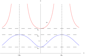
Figure 1: Case A.1.a – three different roots. There is an oscillating non-singular (ONS) solution $x_{-}$ given by (A.7) and a singular solution (of Big-Rip to Big-Rip (BR-BR) type) $x_{+}$ given by (A.8).

A.1.2 $\Delta=0$

Here, there is a double or a triple root. In order to distinguish between these two possibilities, we use the equation (A.4). The roots of the polynomial $V(v)$: $\widetilde{e}_{1}$, $\widetilde{e}_{2}$, $\widetilde{e}_{3}$, must satisfy: $\widetilde{e}_{1}+\widetilde{e}_{2}+\widetilde{e}_{3}=0$. Therefore a triple root of $W(x)=0$ corresponds to a triple root $v=0$ of $V(v)$, with $g_{2}=g_{3}=0$.

Let us investigate the former case first. Obviously, there must exist another real root, but not necessarily positive. That is, $W(x)=a_{3}(x-e_{1})(x-e_{2})^{2}$.

If the double root is a smaller one, then because $a_{3}>0$, we obtain a stable, static solution $x=e_{1}$. If the opposite is true, the same static solution is unstable.

For $e_{2}<e_{1}$ ($e_{1}<1$) we have the following solution with $x\geq e_{1}$ (Fig. 2)

$$x_{0}=e_{1}+(e_{2}-e_{1})\tan^{2}\left[\frac{\sqrt{a_{3}(e_{1}-e_{2})}}{2}(\tau-\tau_{0})\right],$$ (A.9)

which is periodic with a half-period

$$\omega_{1}=\frac{\pi}{\sqrt{a_{3}(e_{1}-e_{2})}}~{}.$$

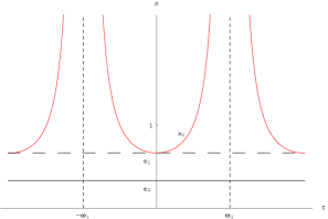
Figure 2: Case A.1.b - the smaller root $e_{2}$ is double. There is a stable static solution (SS) $x=e_{1}$ and a solution $x_{0}$ (BR-BR type) given by (A.9).

In fact, this is valid for both $e_{2}<e_{1}$ and $e_{2}>e_{1}$. However, when $e_{2}>e_{1}$, the solution is no longer periodic, and, upon eliminating the imaginary part of $\tau_{0}$, it is more convenient to write it as (Fig. 3)

$$x_{-} = e_{1}+(e_{2}-e_{1})\tanh^{2}\left[\frac{\sqrt{a_{3}(e_{2}-e_{1})}}{2}(\tau-\tau_{0})\right],$$ (A.10)

when $$e_{1}<1<e_{2}$$

$$x_{+} = e_{1}+(e_{2}-e_{1})\coth^{2}\left[\frac{\sqrt{a_{3}(e_{2}-e_{1})}}{2}(\tau-\tau_{0})\right],$$ (A.11)

when $$e_{2}<1$$.

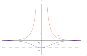
Figure 3: Case A.1.b – the greater root $e_{2}$ is double. There is an unstable static solution (US) $x=e_{2}$ and the two monotonic solutions $x_{\pm}$ given by (A.10) and (A.11). One of them is monotonic non-singular (MNS) and another monotonic to a Big-Rip singularity (MBR).

In terms of the coefficients of the polynomial $W(x)$, it is possible to discern between these two possibilities, as clearly seen from the sign of $W(x_{1})$. The value at the point of inflection is positive when $e_{2}>e_{1}$, and negative otherwise. This relation can be precisely written as: $16g_{3}=-a_{3}^{2}W(x_{1})=\frac{2}{27}a_{3}^{3}(e_{1}-e_{2})^{3}$.

If there is only one triple root $e_{2}$, there is an unstable static solution $x=e_{2}$, and an asymptotic solution (Fig. 4)

$$x_{0}=e_{2}+\frac{4}{a_{3}(\tau-\tau_{0})^{2}}.$$ (A.12)

That is, a “small perturbation” causes the monotonic evolution. Of course, if $e_{2}<0$, only the latter solution remains valid and it is of BB-BR type.

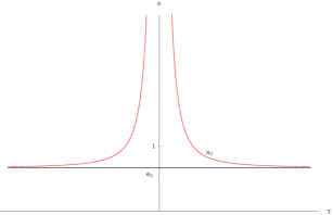
Figure 4: Case A.1.b – one triple root. There is an unstable static solution (US) $x=e_{2}>0$ and a monotonic solution (MBR) $x_{0}$ given by (A.12).

A.1.3 $\Delta<0$

Only one real root exists in this case, and because of (A.2), it must be smaller than unity. Then, there is only one type of solution

$$x_{0}=\frac{4}{a_{3}}\wp(\tau-\tau_{0})-\frac{a_{2}}{3a_{3}},$$ (A.13)

which is singular when the argument $\tau-\tau_{0}=4n{\mathcal{R}e}(\omega_{1}),\;n\in{\bf Z}$ (Fig. 5).

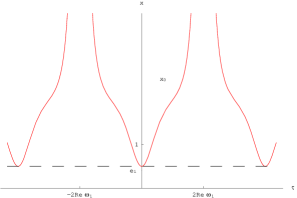
Figure 5: Case A.1.c – one real root exists only. The solution $x_{0}$ is given by (A.13). It is a BR-BR type of solution with no Big-Bang (BB) singularity.

A.2 $a_{3}<0$

A.2.1 $\Delta>0$

This case is, in fact, the same as $a_{3}>0$, with an interchange of possible regions of the evolution. This gives rise to a periodic solution oscillating between the two greater roots $e_{2}\leq x\leq e_{1}$ (Fig. 6)

$$x_{+}=e_{1}+\frac{3a_{3}(e_{1}-e_{2})(e_{1}-e_{3})}{12\wp(\tau-\tau_{0})-(2e_{1}-e_{2}-e_{3})},$$ (A.14)

where the roots have been arranged as before.

Another solution, which in the previous case A.1 was singular, now is also bounded $0\leq x\leq e_{3}$, and is given by (Fig. 6)

$$x_{-}=\frac{4}{a_{3}}\wp(\tau-\tau_{0})-\frac{a_{2}}{3a_{3}}.$$ (A.15)

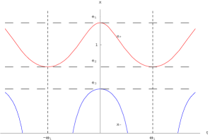
Figure 6: Case A.2.a – three different roots. There is an oscillating non-singular solution (ONS) $x_{+}$ given by (A.14), and a singular solution (of Big-Bang to Big-Crunch (BB-BC) type) $x_{-}$ given by (A.15).

A.2.2 $\Delta=0$

As in the case A.1.b of the $a_{3}>0$ case, we can either have a double or a triple root. Also, we can distinguish between the two double root subcases, using the same formulas as before.

If the root is only double we have a situation similar to what we had before. It can be a greater root, in which case the other root must satisfy $e_{1}>1$, for only then we could have $W(1)=1$. We can only have a stable, static solution $x=e_{2}$, and another one for $0\leq x\leq e_{1}$, given by (Fig. 7):

$$x_{0}=e_{1}+(e_{1}-e_{2})\tan^{2}\left[\frac{\sqrt{|a_{3}|(e_{2}-e_{1})}}{2}(\tau-\tau_{0})\right].$$ (A.16)

(Again, this is valid for all double-root solutions, but $\tau_{0}$ might be complex.)

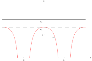
Figure 7: Case A.2.b – the greater root $e_{2}$ is double. There is a stable static solution (SS) $x=e_{1}$ and a BB-BC type singular solution $x_{0}$ given by (A.16).

On the other hand, when $e_{2}<e_{1}$, which requires $e_{1}>1$, there are three possible solutions. One is an unstable static (US) solution $x=e_{2}$. The other two describe the motion between $0\leq x\leq e_{2}$ (asymptotic to the previous one) and $e_{2}\leq x\leq e_{1}$. They are given by (Fig. 8)

$$x_{-} = e_{1}+(e_{2}-e_{1})\coth^{2}\left[\frac{\sqrt{|a_{3}|(e_{1}-e_{2})}}{2}(\tau-\tau_{0})\right],$$ (A.17)

when $$1<e_{2}$$

$$x_{+} = e_{1}+(e_{2}-e_{1})\tanh^{2}\left[\frac{\sqrt{|a_{3}|(e_{1}-e_{2})}}{2}(\tau-\tau_{0})\right],$$ (A.18)

when $$e_{2}<1<e_{1}$$.

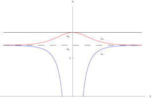
Figure 8: Case A.2.b – the smaller root $e_{2}$ is double. There is an unstable static (US) solution $x=e_{1}$ and the two monotonic solutions $x_{\pm}$ given by (A.17) and (A.18). The former is of monotonic non-singular (MNS) type and the latter is monotonic Big-Bang type (MBB).

When $e_{2}$ is a triple root, there is an unstable, static solution $x=e_{2}$, and a monotonic solution in the form (Fig. 9)

$$x_{0}=e_{2}+\frac{4}{a_{3}(\tau-\tau_{0})^{2}}.$$ (A.19)

In order for condition (A.2) to be satisfied, we must have $e_{2}>1$, as $W(x)$ is positive only for $x<e_{2}$.

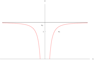
Figure 9: Case A.2.b – one triple root. There is an unstable static (US) solution $x=e_{2}$ and a monotonic Big-Bang (MBB) solution $x_{0}$ given by (A.19).

A.2.3 $\Delta<0$

As in the case 1.c, there is only one real root $e_{1}$, only this time it limits the values of $x$ to $0\leq x\leq e_{1}$. The solution is singular of Big-Bang to Big-Crunch (BB-BC) type (Fig. 10)

$$x_{0}=\frac{4}{a_{3}}\wp(\tau-\tau_{0})-\frac{a_{2}}{3a_{3}},$$ (A.20)

A.3 $a_{3}=0$

This case was studied in the Appendix A of Ref. phantom1 .

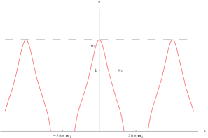
Figure 10: Case 2.c – one real root only. The solution $x_{0}$ is given by (A.20) and is of BB-BC type.

Appendix B General classification of the models which lead to a quartic polynomial in the canonical equation

In this Appendix we consider the canonical equation

$$\left(\frac{\mathrm{d}x}{\mathrm{d}\tau}\right)^{2}=a_{4}x^{4}+a_{3}x^{3}+a_{2}x^{2}+a_{1}x+a_{0}=W(x),$$ (B.21)

and impose the constraint

$$W(1)=a_{4}+a_{3}+a_{2}+a_{1}+a_{0}=1$$ (B.22)

which holds with the same restrictions as in the previous case of Appendix A. In order to make the analysis of the roots easier, we transform (B.22) to the form

$$\frac{1}{a_{4}}W(x-\frac{a_{3}}{4a_{4}})=x^{4}+px^{2}+qx+r.$$ (B.23)

Because of that, it is easier to define a set of auxiliary quantities

$$\delta_{ij}=(e_{i}-e_{j})^{2}~{},$$

where $e_{i}$ are the four roots of the polynomial $W(x)$, and $i,j=1,2,3,4$. It is clear, that the original equation (B.21), and the transformed equation (B.23) have exactly the same values of $\delta$, and general properties of the roots remain the same. Now let $\mathcal{J}$ be the set of all possible values of the symmetric multi-index $ij$. We can further define the quantities:

$$\sigma_{6} = \prod_{\kappa\in\mathcal{J}}\delta_{\kappa},$$

$$\sigma_{5} = \sum_{\kappa\in\mathcal{J}}\delta_{\kappa}^{-1}\prod_{\alpha\in\mathcal{J}}\delta_{\alpha},$$

$$\sigma_{4} = \sum_{\kappa_{1},\kappa_{2}\in\mathcal{J},\kappa_{1}<\kappa_{2}}\delta_{\kappa_{1}}^{-1}\delta_{\kappa_{2}}^{-1}\prod_{\alpha\in\mathcal{J}}\delta_{\alpha},$$

$$\sigma_{3} = \sum_{\kappa_{1},\kappa_{2},\kappa_{3}\in\mathcal{J},\kappa_{1}<\kappa_{2}<\kappa_{3}}\delta_{\kappa_{1}}\delta_{\kappa_{2}}\delta_{\kappa_{3}},$$

$$\sigma_{2} = \sum_{\kappa_{1},\kappa_{2}\in\mathcal{J},\kappa_{1}<\kappa_{2}}\delta_{\kappa_{1}}\delta_{\kappa_{2}},$$

$$\sigma_{1} = \sum_{\kappa\in\mathcal{J}}\delta_{\kappa}.$$ (B.24)

As these quantities are symmetric in the roots, they can be re-expressed by using the coefficients $a_{i}$ or, equivalently, $p$, $q$ and $r$ as

$$\sigma_{6} = -4p^{3}q^{2}-27q^{4}+16p^{4}r+144pq^{2}r-128p^{2}r^{2}+256r^{3},$$

$$\sigma_{5} = -4p^{5}-18p^{2}q^{2}-32p^{3}r-216q^{2}r+192pr^{2},$$

$$\sigma_{4} = 17p^{4}+48pq^{2}+24p^{2}r-112r^{2},$$

$$\sigma_{3} = -28p^{3}-26q^{2}-16pr,$$ (B.25)

$$\sigma_{2} = 22p^{2}+8r,$$

$$\sigma_{1} = -8p.$$

Note that $\sigma_{6}$ can immediately be identified as the original equation’s discriminant. Together with other $\sigma$’s, it determines the behaviour of the roots in the following way:

1. $\sigma_{6}\neq 0$
   There are four distinct roots, with the following subcases:
      $\sigma_{6}<0$ – two complex, conjugate roots, and two real roots,
      $\sigma_{6}>0$ – four real roots, or four complex roots, cojugate in pairs.

2. $\sigma_{6}=0$, $\sigma_{5}\neq 0$
   There is one double, real root, and:
      $\sigma_{5}>0$ – two real roots,
      $\sigma_{5}<0$ – two complex conjugate roots.

3. $\sigma_{6}=0=\sigma_{5}=0$, $\sigma_{4}\neq 0$
   There are two double roots, which for:
      $\sigma_{1}>0$ are real,
      $\sigma_{1}<0$ are complex, conjugate in pairs.

4. $\sigma_{6}=\sigma_{5}=\sigma_{4}=0$, $\sigma_{3}\neq 0$
   There is a triple real root. The fourth root is also real.

5. $\sigma_{6}=\sigma_{5}=\sigma_{4}=0$, $\sigma_{3}=0\Leftrightarrow\sigma_{2}=0\Leftrightarrow\sigma_{1}=0$
   There is a quadruple root – it is necessarily real.

In order to distinguish between the real and complex roots when $\sigma_{6}>0$, we choose to employ the resolvent polynomial of $W(x)$, which appears in the process of factorizing a quartic polynomial into two quadratic ones

$$x^{4}+px^{2}+qx+r=(x^{2}+kx+m)(x^{2}-kx+n).$$

It is essentially the equation determining the value of $k$, as for $w=k^{2}$, the resolvent equation is

$$w^{3}+2pw^{2}+(p^{2}-4r)w-q^{2}=0.$$

Now, in the case of the four real roots, such decomposition is possible in three different ways, as there are three ways of pairing the roots. Hence, there must be three, distinct, positive solutions for $k^{2}$. If, however, the roots are all complex, in order for the coefficients $k,m,n$ to be real, each root must be paired with its conjugate. Thus, there is only one positive solution for $k^{2}$, and the two negative ones. It is easy to distinguish between these possibilities, looking at the positions of the extrema of the resolvent polynomial. In the first case, there must be the two positive ones, and in the second, if any exist, at least one must be negative. Thus, the problem may be reduced to an investigation of the sign of the smallest extremum:

$$w_{-}=\frac{1}{3}(-2p-\sqrt{p^{2}+12r}).$$ (B.26)

If $p^{2}+12r$ is negative, and there are no extrema, only one decomposition is possible. Note that this quantity must be non-negative in all the multiple root cases, as degeneracy of the roots of $W$ implies multiple roots of the resolvent.

In general, when there are no multiple roots, the main equation (B.21), can be solved by using the substitution:

$$\frac{1}{x-e_{i}}=\frac{4v}{W^{\prime}(e_{i})}-\frac{W^{\prime\prime}(e_{i})}{6W^{\prime}(e_{i})},$$ (B.27)

which transforms it into the Weierstrass equation

$$\dot{v}^{2}=4v^{3}-g_{2}v-g_{3}~{},$$ (B.28)

with the following invariants:

$$g_{2} = a_{4}a_{0}-\frac{1}{4}a_{3}a_{1}+\frac{1}{12}a_{2}^{2}$$

$$= a_{4}^{2}(\frac{1}{12}p^{2}+r),$$

$$g_{3} = \frac{1}{6}a_{4}a_{2}a_{0}-\frac{1}{16}a_{4}a_{1}^{2}+\frac{1}{48}a_{3}a_{2}a_{1}-\frac{1}{16}a_{3}^{2}a_{0}-\frac{1}{216}a_{2}^{3},$$ (B.29)

$$= a_{4}^{3}(-\frac{1}{216}p^{3}-\frac{1}{16}q^{2}+\frac{1}{6}pr).$$

This, however, requires the knowledge of the roots, and usually yields too cumbersome formulas, sometimes with explicitly imaginary coefficients. The following solutions were possible to be simplified as a result of the division into the special subcases. Still, the main function $\wp(\tau)$, and its half-periods, are constructed using the invariants (B.29).

B.1 $a_{4}>0$

B.1.1 $\sigma_{6}\neq 0$ – simple roots

Choosing an integration constant by imposing that $x(0)=1$, we obtain a general solution of the form

$$x_{0}=1+$$ (B.30)

$$\frac{\wp^{\prime}(\tau-\tau_{0})+\frac{1}{4}(4a_{4}+a_{3})}{2[\wp(\tau-\tau_{0})-\frac{1}{12}(6a_{4}+3a_{3}+a_{2})]^{2}-\frac{1}{2}a_{4}}+$$

$$\frac{\frac{1}{2}(4a_{4}+3a_{3}+2a_{2}+a1)[\wp(\tau-\tau_{0})-\frac{1}{12}(6a_{4}+3a_{3}+a_{2})]}{2[\wp(\tau-\tau_{0})-\frac{1}{12}(6a_{4}+3a_{3}+a_{2})]^{2}-\frac{1}{2}a_{4}},$$

which is valid for all subcases. However, the behaviour of this solution varies greatly depending on the properties of the roots. The details are given in the following subsections, and are clearly drawn in the figures.

a.1. Four complex roots

The polynomial $W$ is always positive here, and from a simple, geometric investigation it is clear that the condition (B.22) can be satisfied. Only one solution is present, with a possible time reversal $t\rightarrow-t$ applicable in all cases. It reaches both Big-Bang and Big-Rip in finite times (Fig. 11).

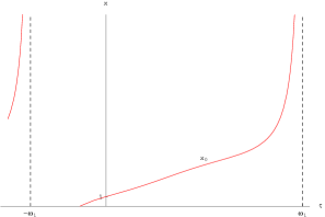
Figure 11: Case B.1.a.1 – four complex roots. The solution $x_{0}$ is given by the formula (B.30) – the evolution starts from Big-Bang and terminates at Big-Rip (BR-BR type).

a.2. Two complex and two real roots

With real roots, the possible domain of $x$ is separated into two regions: $x_{-}\leq e_{1}<e_{2}\leq x_{+}$. However, both solutions are given by the same generic formula (B.30. If we are interested only in physical solutions, then only one “branch” is valid in each case, depending on the position of the roots. Namely, if $1<e_{1}$, we take $x_{-}$, and if $e_{2}<1$, we take $x_{+}$ (Fig. 12). The solution $x_{-}$ starts at Big-Bang reaches the maximum and terminates at Big-Crunch. The solution $x_{+}$ starts at Big-Rip reaches the minimum and terminates at Big-Rip again.

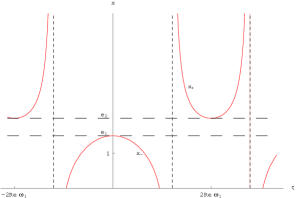
Figure 12: Case B.1.a.2 – two complex and two real roots. There are two solutions $x_{\pm}$ both given by general formula (B.30). The solution $x_{-}$ is of BB-BC type while the the solution $x_{+}$ is of BR-BR type.

a.3. Four real roots

The situation is similar to the case a.2 and with two more roots, there is a third admissible region only. We now have: $x_{-}\leq e_{1}<e_{2}\leq x_{0}\leq e_{3}<e_{4}\leq x_{+}$, depending on which of these intervals the line $x=1$ belongs to. The solutions $x_{-}$ (BB to BC) and $x_{+}$ (BR only), are described by equation (B.30), and $x_{0}$ is obtained, by adding a purely imaginary half-period $\omega_{3}$ to the argument. This last solution is oscillating with a period $2\omega_{1}$, and avoids any singularity when $0<e_{2}$ (Fig. 13).

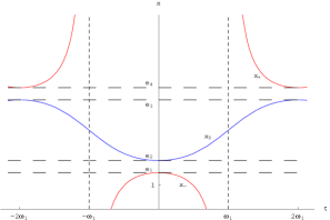
Figure 13: Case B.1.a.3 – four real roots. There are three solutions: $x_{0}$ (oscillating), and $x_{\pm}$ (BR only, BB to BC) given by (B.30) and (B.32), respectively.

B.1.2 $\sigma_{6}=0$ – one double root

b.1. $\sigma_{5}<0$ – two real and two complex roots

With the appearance of multiple roots, the solutions simplify significantly. Firstly, it is possible to express the roots themselves in a suitably short form. Secondly, the elliptic function $\wp$ reduces to a trigonometric or a hyperbolic function.

In this case, the double root is real, and the remaining two roots are complex. Using equation (B.23), we can easily obtain a double root

$$e_{1}=\frac{-3q}{4p+2\sqrt{p^{2}+12r}}-\frac{a_{3}}{4a_{4}},$$ (B.31)

which applied gives an appropriate solution

$$x_{\pm}=\frac{6W_{1}^{\prime\prime}}{W_{1}^{\prime\prime\prime}+\sqrt{3W_{1}^{\prime\prime}W_{1}^{(4)}-W_{1}^{\prime\prime\prime 2}}\sinh\left[\sqrt{\frac{1}{2}W_{1}^{\prime\prime}}(\tau-\tau_{0})\right]},$$ (B.32)

where the index indicates that the value $W(x)$ should be taken at $x=e_{1}$. As in 1.a.2, this formula incorporates both $x_{+}>e_{1}$ and $x_{-}<e_{1}$. Which of these should be used depends on whether $e_{1}<1$ or $1<e_{1}$, respectively. Also, there is an unstable static solution $x_{0}=e_{1}$ and the solutions $x_{\pm}$ which approach it from either Big-Bang or Big-Rip (which differs from standard case of an Einstein Static Universe - Fig. 14).

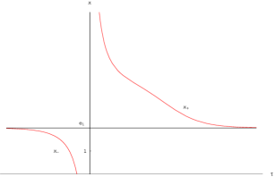
Figure 14: Case B.1.b.1 – two real and two complex roots. There is an unstable static solution $x=e_{1}$ and the two asymptotic solutions $x_{\pm}$ given by (B.32). One of them approaches Big-Bang (MBB type) and another approaches Big-Rip (MBR type).

b.2. $\sigma_{5}>0$ – four real roots

Depending on the relative values of the roots, three situations are possible. Denoting a double root by $e_{1}$, given by the same formula as before, we always have a stable static solution $x_{0}=e_{1}$. Since we know $e_{1}$, it is also possible to obtain the remaining roots, and check which of the following is applicable. If $e_{2}<e_{1}<e_{3}$,

$$x_{\pm}=e_{2}+$$ (B.33)

$$\frac{(e_{2}-e_{1})(e_{2}-e_{3})}{e_{1}-e_{2}+(e_{1}-e_{3})\tan\left[\frac{1}{2}\sqrt{a_{4}(e_{1}-e_{2})(e_{3}-e_{1})}(\tau-\tau_{0})\right]^{2}},$$

with the choice of the + or - “branch” depending on whether $1<e_{2}$, or $e_{3}<1$ (Fig. 15).

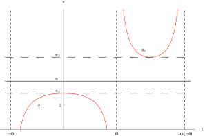
Figure 15: Case B.1.b.2 – the double root is between the other two roots. There is a stable static solution $x=e_{1}$ and the two solutions given by (B.33) (of BB-BC and BR-BR type).

The second possibility is that $e_{1}<e_{2}<e_{3}$, where the solutions in the regions adjacent to $e_{1}$, that is, $0\leq x<e_{1}$ and $e_{1}<x\leq e_{2}$, tend to $e_{1}$ asymptotically, and $x_{0}=e_{1}$ becomes unstable. The respective formulas are (Fig. 16)

$$x_{+}=e_{2}+$$ (B.34)

$$\frac{(e_{2}-e_{1})(e_{2}-e_{3})}{e_{1}-e_{2}+(e_{3}-e_{1})\tanh\left[\frac{1}{2}\sqrt{a_{4}(e_{2}-e_{1})(e_{3}-e_{1})}(\tau-\tau_{0})\right]^{2}},$$

$$x_{-1,2}=e_{2}+$$ (B.35)

$$\frac{(e_{2}-e_{1})(e_{2}-e_{3})}{e_{1}-e_{2}+(e_{3}-e_{1})\coth\left[\frac{1}{2}\sqrt{a_{4}(e_{2}-e_{1})(e_{3}-e_{1})}(\tau-\tau_{0})\right]^{2}}.$$

For a finite value of $\tau$, $x$ reaches infinity and

$$\tau-\tau_{0}=\varpi=\frac{2}{\sqrt{a_{4}(e_{1}-e_{2})(e_{1}-e3)}}\mathrm{artanh}\left(\sqrt{\frac{e_{1}-e_{3}}{e_{1}-e_{2}}}\right).$$

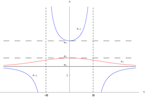
Figure 16: Case B.1.b.2 – the smallest root is double. There is an unstable static (US) solution $x=e_{1}$, and the three other solutions $x_{+}$ (MUS) and $x_{-1,2}$ (MBB, BR-BR) given by (B.1.2) and (B.1.2), respectively.

Lastly, when $e_{2}<e_{3}<e_{1}$, the situation is similar to the previous one, only the asymptotic branch of $x_{-1}$ is now the upper one, with

$$x_{+}=e_{2}+$$ (B.36)

$$\frac{(e_{2}-e_{1})(e_{2}-e_{3})}{e_{1}-e_{2}+(e_{3}-e_{1})\coth\left[\frac{1}{2}\sqrt{a_{4}(e_{1}-e_{2})(e_{1}-e_{3})}(\tau-\tau_{0})\right]^{2}},$$

$$x_{-1,2}=e_{2}+$$ (B.37)

$$\frac{(e_{2}-e_{1})(e_{2}-e_{3})}{e_{1}-e_{2}+(e_{3}-e_{1})\tanh\left[\frac{1}{2}\sqrt{a_{4}(e_{1}-e_{2})(e_{1}-e_{3})}(\tau-\tau_{0})\right]^{2}},$$

and the static solution $x_{0}=e_{1}$ is also unstable (Fig. 17). Here we have

$$\varpi=\frac{2}{\sqrt{a_{4}(e_{1}-e_{2})(e_{1}-e_{3})}}\mathrm{artanh}\left(\sqrt{\frac{e_{1}-e_{2}}{e_{1}-e_{3}}}\right).$$

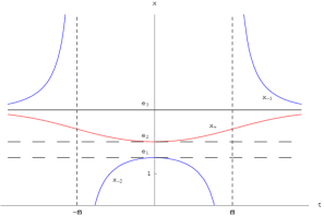
Figure 17: Case B.1.b.2 – the greatest root is double. There is an unstable static solution $x=e_{1}$ and the other solutions $x_{+}$ (oscillating) and $x_{-1,2}$ (from BB to BC, bounce to BR) given by (B.1.2) and (B.1.2), respectively.

B.1.3 $\sigma_{6}=\sigma_{5}=0$, $\sigma_{4}\neq 0$ – two double roots

c.1. $\sigma_{1}>0$ – four real roots

The formula for the roots is further simplified to:

$$e_{1,2}=-\frac{a_{3}}{4a_{4}}\mp\sqrt{-\frac{1}{2}p}.$$ (B.38)

Here $-2p$ is equal to the discriminant of the equation $(x-e_{1})(x-e_{2})$, and is always positive. As for the solutions, we have two static, unstable solutions corresponding to $x_{0}=e_{1,2}$, and the remaining two are given by (Fig. 18)

$$x_{+}=e_{1}+$$

$$\sqrt{-\frac{1}{2}p}\left\{1+\tanh\left[\sqrt{-\frac{1}{2}pa_{4}}(\tau-\tau_{0})\right]\right\},$$ (B.39)

$$x_{-1,2}=e_{1}+$$

$$\sqrt{-\frac{1}{2}p}\left\{1+\coth\left[\sqrt{-\frac{1}{2}pa_{4}}(\tau-\tau_{0})\right]\right\}.$$ (B.40)

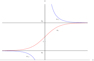
Figure 18: Case B.1.c.1 – four real roots, two of them are double. There are two unstable static solutions $x_{0}=e_{1},x_{0}=e_{2}$ and the three other solutions $x_{+}$ and $x_{-1,2}$ given by (B.39) and (B.40), respectively. The solution $x_{+}$ asymptotes from one unstable static solution to the other (MUS-MUS type) while $x_{-1}$ is of MBR type and $x_{-2}$ is of MBB type.

c.2. $\sigma_{1}<0$ – four complex roots

Similarly to 1.a.1, the polynomial $W$ is always positive, but the solution is simplified to

$$x_{0}=-\frac{a_{3}}{4a_{4}}+\sqrt{\frac{1}{2}p}\,\tan\left[\sqrt{\frac{1}{2}pa_{4}}(\tau-\tau_{0})\right],$$ (B.41)

with $p$ always positive this time (Fig. 19).

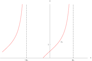
Figure 19: Case B.1.c.2 – four complex roots. The solution $x_{0}$ is given by (B.41) and is of BB-BR type.

B.1.4 $\sigma_{6}=\sigma_{5}=\sigma_{4}=0$, $\sigma_{3}\neq 0$ – one triple root

The multiple root now becomes:

$$e_{1}=-\frac{a_{3}}{4a_{4}}-\frac{1}{2}\sqrt[3]{q},$$ (B.42)

and the fourth root is:

$$e_{2}=-\frac{a_{3}}{4a_{4}}+\frac{3}{2}\sqrt[3]{q}.$$ (B.43)

There are two subcases, with $e_{1}<e_{2}$ and $e_{1}>e_{2}$, respectively, but the solution for both “branches” in each subcase is given by the same formula:

$$x_{\pm}=\frac{a_{4}e_{1}(e_{1}-e_{2})^{2}(\tau-\tau_{0})^{2}-4e_{2}}{a_{4}(e_{1}-e_{2})^{2}(\tau-\tau_{0})^{2}-4}.$$ (B.44)

Infinite $x$ is reached for a finite value of $\tau$:

$$\tau-\tau_{0}=\varpi=\frac{2}{\sqrt{|a_{4}|}|e_{1}-e_{2}|}.$$

There is also the unstable, static solution $x_{0}=e_{1}$ (Figs. 20,21).

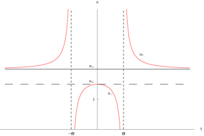
Figure 20: Case B.1.d – one triple root which is greater than a single root. There is an unstable static solution $x_{0}=e_{1}$ and the other solutions $x_{\pm}$ (BB-BC and MBR type) are given by (B.44).

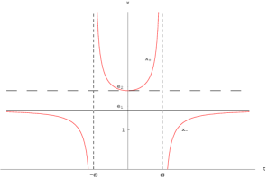
Figure 21: Case B.1.d – one triple root which is smaller than a single root. There is an unstable static solution $x_{0}=e_{1}$ and the other two solutions $x_{\pm}$ (BR to BR, BB only) are given by (B.44).

B.1.5 $\sigma_{6}=\sigma_{5}=\sigma_{4}=\sigma_{1}=0$ – one quadruple root

This is the simplest case, immediately integrable to:

$$x_{\pm}=e_{1}+\frac{1}{\sqrt{a_{4}}(\tau-\tau_{0})},$$ (B.45)

where the root is:

$$e_{1}=-\frac{a_{3}}{4a_{4}}.$$ (B.46)

Again, we have two “branches” separated by the static, unstable solution $x_{0}=e_{1}$ (Fig. 22).

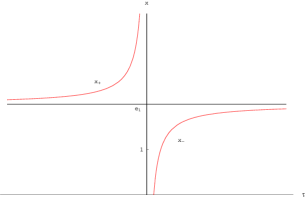
Figure 22: Case B.1.e – one quadrupole root. There is an unstable static (US) solution and the solutions $x_{\pm}$ given by (B.45. They are of MBR and MBB type.

B.2 $a_{4}<0$

B.2.1 $\sigma_{6}\neq 0$ – simple roots

a.1. Four complex roots

This case is clearly impossible, as the polynomial $W$ is everywhere negative.

a.2. Two complex and two real roots

There is only one possible solution, as $W(x)\geq 0$ when $e_{1}\geq x\geq e_{2}$, where $e_{1},e_{2}$ are the real roots. The general formula (B.30) still holds, but the behaviour of the solution is qualitatively different. It has a real period of $2\omega_{1}$, defined as before, and avoids any singularity, provided that $e_{1}>0$ (Fig. 23).

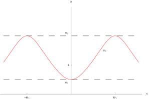
Figure 23: Case B.2.a.2 – two complex and two real roots. This is an oscillating non-singular (ONS) solution $x_{0}$, given by the formula (B.30).

a.3. Four real roots

There are only two possible solutions when $e_{1}<1<e_{2}$ or $e_{3}<1<e_{4}$. They both are also given by the general formula (B.30), independently in each case. They are oscillating, and moreover, and have the same period $2\omega_{1}$, so that, if $0<e_{1}$ no singularity is present at all (Fig. 24).

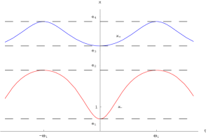
Figure 24: Case B.2.a.3 – four real roots. This is a “double” oscillating case, which means we have the two oscillating solutions $x_{\pm}$ of the same period $2\omega_{1}$ given by the formula (B.32). They are non-singular provided $e_{1}>0$.

B.2.2 $\sigma_{6}=0$ – one double root

b.1. $\sigma_{5}<0$ – two real and two complex roots

There is only one possible solution: $x_{0}=e_{1}$, with the root given by (B.31). As $W$ is negative everywhere else, this solution is stable.

b.2. $\sigma_{5}>0$ – four real roots

Here, there are two subcases, both with the static solution $x_{0}=e_{1}$. The first one occurs when $e_{2}<e_{1}<e_{3}$, and there are two other solutions asymptotic to $x_{0}$ (Fig. 25)

$$x_{+}=e_{2}+$$ (B.47)

$$\frac{(e_{2}-e_{1})(e_{2}-e_{3})}{e_{1}-e_{2}+(e_{3}-e_{1})\coth\left[\frac{1}{2}\sqrt{|a_{4}|(e_{1}-e_{2})(e_{3}-e_{1})}(\tau-\tau_{0})\right]^{2}},$$

$$x_{-}=e_{2}+$$ (B.48)

$$\frac{(e_{2}-e_{1})(e_{2}-e_{3})}{e_{1}-e_{2}+(e_{3}-e_{1})\tanh\left[\frac{1}{2}\sqrt{|a_{4}|(e_{1}-e_{2})(e_{3}-e_{1})}(\tau-\tau_{0})\right]^{2}}.$$

If $e_{1}<e_{2}$ or $e_{3}<e_{1}$, $x_{0}$ becomes stable, and there is only one other oscillating solution between $e_{2}$ and $e_{3}$ (Fig. 26)

$$x_{+}=e_{2}+$$ (B.49)

$$\frac{(e_{2}-e_{1})(e_{2}-e_{3})}{e_{1}-e_{2}+(e_{1}-e_{3})\tan\left[\frac{1}{2}\sqrt{|a_{4}|(e_{1}-e_{2})(e_{1}-e_{3})}(\tau-\tau_{0})\right]^{2}}.$$

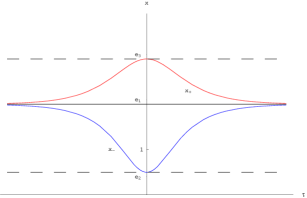
Figure 25: Case B.2.b.2 – one double root which is between the two single roots. There is an unstable static (US) solution $x_{0}=e_{1}$ and the two asymptotic solutions $x_{\pm}$ given by (B.47) and (B.48).

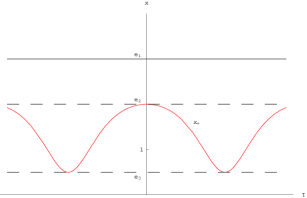
Figure 26: Case B.2.b.2 – one double root greater than the two single roots. There is a stable static (SS) solution $x_{0}=e_{1}$ and an oscillating solution $x_{+}$ (ONS type) given by (B.49).

B.2.3 $\sigma_{6}=\sigma_{5}=0$, $\sigma_{4}\neq 0$ – two double roots

c.1. $\sigma_{1}>0$ – four real roots

The only possible solutions here, are two static, stable ones: $x_{0}=e_{1,2}$. The roots are given by formula (B.38).

c.2. $\sigma_{1}<0$ – four complex roots

$W$ is negative for all $x$, so this case is impossible.

B.2.4 $\sigma_{6}=\sigma_{5}=\sigma_{4}=0$, $\sigma_{3}\neq 0$ – one triple root

Essentially this is just one case, but depending on the position of the triple root, the non-static solution

$$x_{\pm}=\frac{4e_{2}-a_{4}e_{1}(e_{1}-e_{2})^{2}(\tau-\tau_{0})^{2}}{4-a_{4}(e_{1}-e_{2})^{2}(\tau-\tau_{0})^{2}},$$ (B.50)

has either a maximum, for $e_{1}<e_{2}$, or a minimum, for $e_{1}>e_{2}$. Also, $x_{0}=e_{1}$ is an unstable static solution (Figs. 27,28).

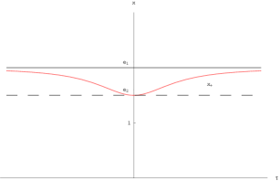
Figure 27: Case B.2.d – one triple root greater than a single root. There is an unstable static (US) solution $x_{0}=e_{1}$ and a monotonic solution $x_{+}$ given by (B.50) which has a minimum.

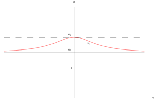
Figure 28: Case B.2.d – one triple root smaller that a single root. There is an unstable static solution $x_{0}=e_{1}$ and a monotonic solution $x_{+}$ given by (B.50) which has a maximum.

B.2.5 $\sigma_{6}=\sigma_{5}=\sigma_{4}=\sigma_{1}=0$ – one quadruple root

There is only one point where $W$ is not negative, thus yielding just the stable, static solution of $x_{0}=e_{1}$, where $e_{1}$ is given by the formula (B.46).

B.3 $a_{4}=0$

This case is essentially reduced to a cubic polynomial case considered in the Appendix A.

References

- (1) A. Vilenkin, Phys. Rep. 121 (1985), 265; T. Vachaspati, and A. Vilenkin, Phys. Rev. D35 (1987), 1131.
- (2) M.P. Da̧browski, and J. Stelmach, Astron. Journ. 97 (1989), 978 (astro-ph/0410334).
- (3) S. Perlmutter et al., Astroph. J. 517, (1999) 565; A. G. Riess et al. Astron. J. 116 (1998) 1009; A.G. Riess et al., Astroph. J. 560 (2001), 49; ibidem 594 (2003), 1.
- (4) J.L. Tonry et al., Astroph. J. 594 (2003), 1; M. Tegmark et al., Phys. Rev. D69 (2004), 103501.
- (5) R.R. Caldwell, Phys. Lett. B545 (2002), 23 (astro-ph/9908168).
- (6) S.M. Carroll, M. Hofman, and M. Trodden, Phys. Rev. D68 (2003), 023509; S.D.H. Hsu, A. Jenkins, and M.B. Wise, Phys. Lett. B597 (2004), 270.
- (7) S. Nojiri, and S.D. Odintsov, Phys. Lett. B595 (2004), 1; Phys. Rev. D70 (2004), 103522.
- (8) S.W. Hawking, and G.F.R. Ellis, The Large-scale Structure of Space-time (Cambridge Univ. Press, 1999).
- (9) M. Visser, Lorentzian Wormholes (Springer, New York, 1996).
- (10) C. Csaki, N. Kaloper, and J. Terning, Ann. Phys. (N.Y.) 317 (2005), 410.
- (11) J.D. Barrow, Class. Quantum Grav. 21, L79 (2004); ibidem 21, 5619 (2004), J.D. Barrow, and Ch. Tsagas, Class. Quantum Grav. 22 (2005), 1563; L. Fernandez-Jambrina, and R. Lazkoz, Phys. Rev. D70, 121503 (2004).
- (12) M.P. Da̧browski, W. Godłowski, and M. Szydłowski, Intern. Journ. Mod. Phys. D 13 (2004), 1669.
- (13) J.D. Barrow, Nucl. Phys. B310 (1988), 743.
- (14) M.D. Pollock, Phys. Lett. B215 (1988), 635.
- (15) B. Boisseau, G. Esposito-Farése, D. Polarski, and A.A. Starobinsky, Phys. Rev. Lett. 85 (2000), 2236; A.A. Starobinsky, Grav. Cosmol. 6 (2000), 157.
- (16) A. Kehagias, and E. Kiritsis, JHEP 9911 (1999), 022.
- (17) T. Chiba, T. Okabe, and M. Yamaguchi, Phys. Rev. D62 (2000), 023511.
- (18) S. Hannestad, and E. Mörstell, Phys. Rev. D 66, 063508 (2002)
- (19) P.H. Frampton, Phys. Lett. B557 (2003), 135.
- (20) P.H. Frampton, Phys. Lett. B 555 (2003), 139.
- (21) P.H. Frampton, and T. Takahashi, Phys. Lett. B557 (2003), 135.
- (22) B. McInnes, JHEP 0208 (2002), 029.
- (23) S.M. Carroll, M. Hoffman, and M. Trodden, Phys. Rev. D 68 (2003), 023509.
- (24) A. Melchiorri, L. Mersini, C.J. Odman, and M. Trodden, Phys. Rev. D 68 (2003) 043509.
- (25) L. Mersini, M. Bastero-Gil and P. Kanti, Phys. Rev. D64 (2001), 043508.
- (26) M. Bastero-Gil, P.H. Frampton and L. Mersini, Phys. Rev. D65 (2002), 106002.
- (27) M. Abdalla, S. Nojiri, and S. Odintsov, Class. Quantum Grav. 22 (2005), L35.
- (28) J.K. Erickson, R.R. Caldwell, P.J. Steinhardt, C. Armendariz-Picon, and V. Mukhanov, Phys. Rev. Lett. 88 (2002), 121301.
- (29) J. Hao, and X. Li, Phys. Rev. D 68 (2003), 043501.
- (30) X. Li, and J. Hao, Phys. Rev. D69 (2004) 107303.
- (31) P. Singh, M. Sami, and N. Dadhich, Phys. Rev. D 68 (2003), 043501.
- (32) S. Nojiri, and D. Odintsov, Phys. Lett. B562 (2003), 147.
- (33) S. Nojiri, and D. Odintsov, Phys. Lett. B565 (2003), 1.
- (34) S. Nojiri, and D. Odintsov, Phys. Lett. B571 (2003), 1.
- (35) S. Nojiri, and S.D. Odintsov, Phys. Lett. B576 (2003), 5.
- (36) M. Szydłowski, W. Czaja, and A. Krawiec, Phys. Rev. E/bf 72 (2005), 036221.
- (37) V.K. Onemli, and R.P. Woodard, Class. Quantum Grav. 19 (2002), 4607; Phys. Rev. D 70 (2004), 107301; T. Brunier, V.K. Onemli, and R.P. Woodard, Class. Quantum Grav. 22 (2005), 59.
- (38) P.F. Gonzalez-Diaz, Phys. Rev. D 68 (2003), 021303; ibid D 69 (2004), 063522; Phys. Lett. B 586 (2004), 1; e-print: hep-th/0411070, P.F. Gonzalez-Diaz, and C.L. Sigüenza, Nucl. Phys. B 697 (2004), 363.
- (39) B.B. Feng, X-L. Wang, and X-M. Zhang, Phys. Lett. B607 (2005), 35; Z-K. Guo, Y-S. Piao, and Y-Z. Zhang, Phys. Lett. B594 (2004), 247; B.B. Feng, M. Li, Y-S.Piao, and X-M. Zhang, e-print: astro-ph/0407432, Z-K. Guo, Y-S. Piao, X-M. Zhang, and Y-Z. Zhang, Phys. Lett. B608 (2005), 177; Z-K. Guo, and Y-Z. Zhang, Phys. Rev. D71 (2005), 023501.
- (40) R-G. Cai and A. Wang, JCAP 0503 (2005), 002.
- (41) G. Calcagni, Phys. Rev. D71 (2005), 023511; gr-qc/0410111.
- (42) M.P. Da̧browski, Journ. Math. Phys. 34, 1447 (1993).
- (43) M.P. Da̧browski, Astroph. J. 447, 43 (1995).
- (44) M.P. Da̧browski, Phys. Rev. D 71 (2005), 103505.
- (45) M.P. Da̧browski, T. Stachowiak and M. Szydłowski, Phys. Rev. D 68, 103519 (2003).
- (46) K.A. Meissner and G. Veneziano, Phys. Lett. B267 (1991), 33; Mod. Phys. Lett. A6 (1991), 1721.
- (47) J.E. Lidsey, D.W. Wands, and E.J. Copeland, Phys. Rep. 337 (2000), 343.
- (48) L.P. Chimento Phys. Rev. D65 (2002), 063517.
- (49) J.M. Aguirregabiria, L.P. Chimento, A.S. Jacubi, and R. Lazkoz, Phys. Rev. D67 (2003), 083518.
- (50) J. Khoury et al, Phys. Rev. D 64 (2001), 123522; P.J. Steinhardt, and N. Turok, Phys. Rev. D 65 (2002), 126003; J. Khoury, P.J. Steinhardt, and N. Turok, Phys. Rev. Lett. 92 (2004), 031302.
- (51) J.E. Lidsey, Phys. Rev. D 70 (2004), 041302.
- (52) M. Visser, Class. Quantum Grav. 21 (2004), 2603; U. Alam, V. Sahni, T.D. Saini, and A.A. Starobinsky, Mon. Not. R. Astron. Soc. 344 (2003), 1057.
- (53) R.R. Caldwell, and M. Kamionkowski, J. Cosmol. Astropart. Phys. 0409 (2004), 009.
- (54) S. Weinberg, Gravitation and Cosmology (Wiley, New York, 1972).
- (55) R. Coquereaux, and A. Grossmann Ann. Phys. (N.Y.) 143 (1982), 296; M.P. Da̧browski, and J. Stelmach, Ann. Phys (N. Y.) 166 (1986), 422; M.P. Da̧browski, Ann. Phys (N. Y.) 248 (1996) 199; Coquereaux and Grossmann, astro-ph/0101369.
- (56) M.Abramovitz, and I.A. Stegun, Handbook of Mathematical Functions (Dover, New York, 1964).
- (57) K. Lake, Class. Quantum Grav. 21 (2004), L129.
- (58) J. Kristian, and R.K. Sachs, Astrophys. J. 143 (1966), 379.
- (59) G.F.R. Ellis, and M.A.H. MacCallum, Commun. Math. Phys. 19 (1970), 31.