UB-ECM-PF-04/29

KUL-TF-04/31

Rotating Solutions of Non-relativistic String Theory
Joaquim Gomis ^†,1 and Filippo Passerini ^∗,2

^† Departament ECM, Facultat de Física,
Universitat de Barcelona and Institut de Física d’Altes Energies,
Diagonal 647, E-08028 Barcelona, Spain
^∗ Instituut voor Theoretische Fysica,
Katholieke Universiteit Leuven,
Celestijnenlaan 200D, B-3001 Leuven, Belgium

Abstract

We construct classical rotating solutions of Non-relativistic String Theory. The relation among the energy and angular momenta for these solutions is of the type $E=J^{2}$. Some of the solutions saturate a BPS bound for the energy, they are ${1\over 4}$ BPS supersymmetric configurations.

PACS number: 11.25.-w

Keywords: non-relativistic strings, classical solutions.  ¹ E-mail: gomis@ecm.ub.es
² E-mail: Filippo.Passerini@fys.kuleuven.ac.be

1 Introduction

Non-relativistic strings (NR ) in flat transverse space with a non-trivial spectrum were introduced in [1][2], in the static gauge they become free theories [3]. The actions of NR strings and branes can be constructed as Wess-Zumino terms [4] of the underlying Galilei groups using the method of non-linear realizations for space-time groups [5] [6].

NR superstring theories in flat transverse space were recently analyzed in [7]. The action was obtained by performing a suitable non relativistic limit of Green-Schwarz type IIA string. These NR superstring theories have gauge diffeomorphism and kappa symmetry.

We hope the study of NR string theory could be usefull to find a new sector of the theory where the AdS/CFT correspondence can be tested.

In this paper we consider NR bosonic string in a curved transverse space in terms of a Polyakov type action. In the static gauge case, we derive a BPS bound for the energy. This theory is conformal at quantum level if the transverse metric is Ricci flat.

We study rotating solutions of the classical equations of motion for the flat case and for the singular conifold [8]. For the case of the conifold the solutions we found have three angular momenta. The relation among the energy and angular momenta is of non-relativistic type $E\sim J^{2}$ where $J$ represents the angular momenta.

We also analyze the supersymmetric properties of the bosonic solutions we have found by studying the conditions imposed by the kappa symmetry and supersymmetry of the NR superstring [7].

The organization of the paper is as follows. In section 2 we introduce Polyakov form NR string and derive a BPS bound for the energy. In section 3 we find rotating solutions of NR string in flat space time. In section 4 we consider solutions in the case of a singular conifold. In section 5 we study the supersymmetric properties of our solutions. We also give some conclusions in section 6.

2 Non-relativistic strings in transverse curved backgrounds and BPS bound

We study a non-relativistic string in a $d$-dimensional space-time, with coordinates $x^{\mu}$, $\mu=0,1$, along the string and transverse coordinates $X^{a}$, $a=2,\ldots,d-1$. The $d$-dimensional metric is

$$g_{MN}=\left(\begin{array}[]{cc}\eta_{\mu\nu}&0\\ 0&G_{ab}(X^{a})\end{array}\right).$$ (2.3)

The $\eta_{\mu\nu}$ is the $2$-dimensional Minkowski metric with signature $(-,+)$ and $G_{ab}(X^{a})$ is a metric on some $(d-2)$-dimensional Riemannian manifold ${\cal M}$.

The action of NR string is given by

$$S=-{1\over 2}T\int d^{2}\sigma\sqrt{-\det g}\,g^{ij}\partial_{i}X^{a}\partial_{j}X^{b}G_{ab}$$ (2.4)

where $g^{ij}$ is the inverse of the two dimensional metric

$$g_{ij}=\partial_{i}x^{\mu}\partial_{j}x^{\nu}\eta_{\mu\nu},$$ (2.5)

the worldsheet coordinates are $\tau$ and $\sigma$, $\sigma^{i}=(\tau,\sigma),i=1,2$.

The action is invariant under 2d diffeomorphism of the world sheet. In order to have a consistent non relativistic string theory at quantum level we have to consider the coordinate $x^{1}$ toroidally compactified [1][2], i.e.:

$$x^{1}\backsim x^{1}+2\pi R.$$ (2.6)

We now analyze the dynamics of non relativistic strings at classical level by using the Hamiltonian formalism. Let us indicate by $p_{\mu}$ the canonical momenta associated to the longitudinal coordinates $x^{\mu}$ and $P_{a}$ the transverse momenta. As a consequence of the gauge symmetry of the action (2.4), the canonical variables satisfy the following two primary first class constraints:

$$V_{0} = p_{\mu}\;\varepsilon^{\mu\rho}\eta_{\rho\nu}\;{x^{\prime}}^{\nu}+\frac{1}{2}\left(\frac{P_{a}P_{b}}{T}G^{ab}(X)+{X^{\prime}}^{a}{X^{\prime}}^{b}TG_{ab}(X)\right)\sim 0,$$ (2.7)

$$V_{1} = p_{\mu}{x^{\prime}}^{\mu}+P_{a}{X^{\prime}}^{a}\sim 0.$$ (2.8)

The Dirac hamiltonian is:

$$H_{D}=\int d\sigma\left[\lambda_{0}V_{0}+\lambda_{1}V_{1}\right]$$ (2.9)

where $\lambda_{0},\lambda_{1}$ are arbitrary functions of the world sheet coordinates $\sigma^{i}$.

If we write these arbitrary functions in terms of an auxiliary two dimensional metric $\gamma_{ij}$, $\lambda_{0}=\frac{\sqrt{-\gamma}}{\gamma_{11}},\lambda_{1}=\frac{\gamma_{01}}{\gamma_{11}}$ we will find a gauge invariant Polyakov’s formulation of this non-relativistic string. In fact if we consider the first order action

$${\tilde{S}}_{P}=\int d^{2}\sigma\left[p_{\mu}{\dot{x}}^{\mu}+P_{a}{\dot{X}}^{a}\right]-\int d\tau H_{D}$$ (2.10)

and we eliminated the momenta $P_{a}$ we get

$$S_{P}=\int d^{2}\sigma\Bigg{[}-\frac{T}{2}\sqrt{-\gamma}\gamma^{ij}\partial_{i}X^{a}\partial_{j}X^{b}G_{ab}+p_{\mu}(\dot{x}^{\mu}-\frac{\sqrt{-\gamma}}{\gamma_{11}}\varepsilon^{\mu\rho}\ \eta_{\rho\nu}\;{x^{\prime}}^{\nu}-\frac{\gamma_{01}}{\gamma_{11}}{x^{\prime}}^{\mu})\Bigg{]}.$$ (2.11)

This action is invariant under 2d diffeomorphism

$$\delta x^{\mu} = \xi^{k}\partial_{k}x^{\mu}$$ (2.12)

$$\delta p_{\mu} = \partial_{k}(\xi^{k}p_{\mu})+p_{\mu}(-{\dot{\xi}}^{0}+{\xi^{\prime}}^{0}\frac{\gamma_{01}}{\gamma_{11}})+p^{\nu}\varepsilon_{\nu\mu}{\xi^{\prime}}^{0}\frac{\sqrt{-\gamma}}{\gamma_{11}}$$ (2.13)

$$\delta X^{a} = \xi^{k}\partial_{k}X^{a}$$ (2.14)

$$\delta\gamma_{ij} = {\cal L}_{\xi}\gamma_{ij}$$ (2.15)

where ${\cal L}_{\xi}$ is the Lie derivative along $\xi$. The action is also invariant under gauge Weyl transformations of the auxiliary metric $\gamma_{ij}$.

If we choose the conformal gauge $\sqrt{-\gamma}\gamma^{ij}=\eta^{ij}$, the action becomes

$$S_{P}=\int d^{2}\sigma\left[-\frac{T}{2}\eta^{ij}\partial_{i}X^{a}\partial_{j}X^{b}G_{ab}+p_{\mu}(\dot{x}^{\mu}-\varepsilon^{\mu\rho}\ \eta_{\rho\nu}\;{x^{\prime}}^{\nu})\right].$$ (2.16)

The equations of motion in the conformal gauge are

$$0 = \eta^{ij}\partial_{i}\partial_{j}X^{a}+\Gamma^{a}_{bc}\eta^{ij}\partial_{i}X^{b}\partial_{j}X^{c}$$ (2.17)

$$0 = \dot{x}^{\mu}-\varepsilon^{\mu\rho}\ \eta_{\rho\nu}\;{x^{\prime}}^{\nu}$$ (2.18)

$$0 = \dot{p}_{\mu}-\varepsilon^{\nu\rho}\ \eta_{\rho\mu}\;{p^{\prime}}_{\nu}$$ (2.19)

where $\Gamma^{a}_{bc}$ are the Christoffel symbols of the metric $G_{ab}$. From (2.18) we deduce that the longitudinal coordinates verify the relations $\dot{x}x^{\prime}=0$ and ${\dot{x}}^{2}+{x^{\prime}}^{2}=0$.

The boundary conditions are the same as the ones considered for the flat space case [3], i.e. for a closed string

$$x^{\mu}(\tau,\sigma+2\pi)=x^{\mu}(\tau,\sigma)+2\pi nR\delta^{\alpha}_{1}\qquad X^{a}(\tau,\sigma+2\pi)=X^{a}(\tau,\sigma)$$ (2.20)

where $n\in\mathbb{Z}$ is the winding number of the string.
For an open string

$$x^{\prime 0}|_{\sigma=\pi}=x^{\prime 0}|_{\sigma=0}=0\qquad x^{1}(\sigma=0)=0\qquad x^{1}(\sigma=\pi)=2\pi nR$$

$$X^{\prime a}_{N}|_{\sigma=\pi}=X^{\prime a}_{N}|_{\sigma=0}=0\qquad\dot{X}^{b}_{D}|_{\sigma=\pi}=\dot{X}^{b}_{D}|_{\sigma=0}=0,$$ (2.21)

also in this case $n\in\mathbb{Z}$ .

If we introduce the coordinates $\gamma=X^{0}+X^{1},\bar{\gamma}=X^{0}-X^{1},\beta=p_{0}+p_{1},\bar{\beta}=p_{0}-p_{1}$ the first order part of the action (2.16) is the conformal (2,2) $\beta\gamma$ system introduced in [1]. Therefore our NR string will be conformal invariant at quantum level if the metric $G_{ab}$ is Ricci flat [9] and the spacetime dimension is 26 [1] like for the ordinary bosonic relativistic string.

To solve the classical equations of motion is convenient to work in the static gauge. We fix this gauge by imposing two gauge fixing constraints:

$$\Phi_{0}\equiv x^{0}-K\tau=0\qquad\Phi_{1}\equiv x^{1}-K\sigma=0$$ (2.22)

where $K$ is a constant. These constraints make the constraints (2.7) (2.8) second class, they are stationary if $\lambda_{0}=1,\lambda_{1}=0$. Therefore the static gauge is included in the conformal gauge. In the static gauge the transverse degrees of freedom, $(X^{a},P_{a})$, are the independent degrees of freedom of the NR string. The dynamics is given by (2.17).

The momenta ${\cal P}_{1}$ along the string, in the static gauge, using the constraints (2.8) is given by

$${\cal P}_{1}=-\frac{1}{K}\int d\sigma\left(P_{a}{X^{\prime}}^{a}\right)$$ (2.23)

and the energy is

$$E=\frac{1}{K}\int d\sigma\left(\frac{(P)^{2}}{2T}+\frac{T(X^{\prime})^{2}}{2}\right)$$ (2.24)

where we have used the constraint (2.7). Note that the energy can be written as

$$E=\int d\sigma\frac{(P^{a}\pm TX^{\prime a})^{2}}{2TK}\pm{\cal P}_{1}=\int d\sigma\frac{T(\dot{X}^{a}\pm X^{\prime a})^{2}}{2K}\pm{\cal P}_{1}.$$ (2.25)

Therefore ${\cal P}_{1}$ is the BPS bound

$$E\geq\pm{\cal P}_{1}\geq 0,$$ (2.26)

the bound is saturated by the BPS configurations

$$\dot{X}^{a}\pm X^{\prime a}=0.$$ (2.27)

The configurations that satisfy the BPS equation (2.27) verify also the second order equations of motion (2.17).

3 Classical Solutions for NR strings in flat space time

We now analyze non relativistic strings in flat transverse space, i.e. we consider $G_{ab}(X^{a})=\delta_{ab}$. The equations of motion (2.17) simplify to:

$$\ddot{X}^{a}=X^{\prime\prime a}.$$ (3.1)

Here we are interested in solutions of (3.1) describing rotating strings, i.e. solutions with angular momentum different from zero. The component of the angular momentum perpendicular to the $X^{a}-X^{b}$ plane is:

$$J^{ab}=\int d\sigma\left(X^{a}P^{b}-X^{b}P^{a}\right).$$ (3.2)

3.1 Closed Strings

We now consider solutions of the equations (3.1) satisfying boundary conditions for closed strings (2.20). To satisfy the boundary conditions for the longitudinal coordinates we have to fix $K=nR$ in the static gauge constraints (2.22).

The simplest solution describing a rotating closed string is:

$$x^{0}=nR\tau\qquad X^{2}=A\sin(\omega\sigma)\sin\left(\omega\tau\right)$$

$$x^{1}=nR\sigma\qquad X^{3}=A\sin(\omega\sigma)\cos\left(\omega\tau\right)$$ (3.3)

where $\omega\in\mathbb{Z}$ and $A$ is a dimensional constant, $[A]=L$; these conventions are valid also for the following solutions. The (3.3) describes a circular string with angular momentum perpendicular to the $X^{2}-X^{3}$ plane (figure 1).

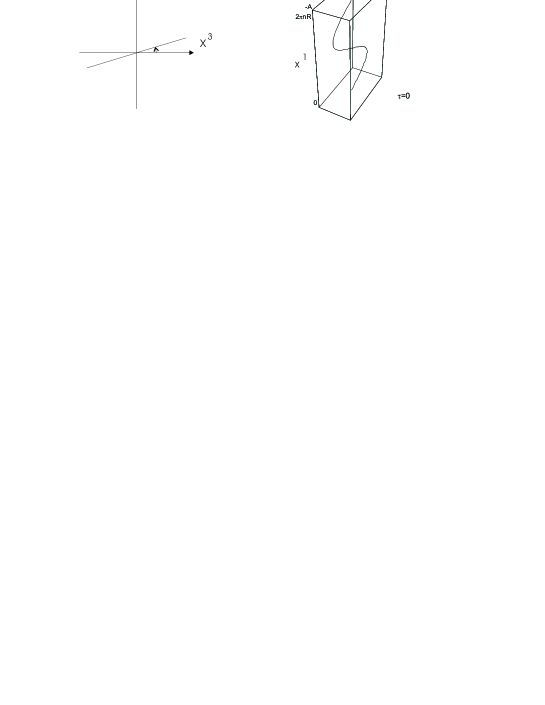
Figure 1: String described by solution (3.3) when $\omega=1$

The velocity modulus of the points of the string is:

$$v^{2}=\left(\frac{\partial X^{2}}{\partial x^{0}}\right)^{2}+\left(\frac{\partial X^{3}}{\partial x^{0}}\right)^{2}=\left(\frac{\omega A}{nR}\right)^{2}\left(\sin(\omega\sigma)\right)^{2}\qquad v_{max}=\frac{A\omega}{nR}\qquad.$$ (3.4)

Like for the relativistic case the turning points are the faster points, but in this case the maximum velocity is not limited by the velocity of light, which in natural units is $v=1$. This is a typical feature of non relativistic theory. By using (2.24) and (3.2) we find:

$$E=\frac{J^{2}}{TA^{2}\pi nR}.$$ (3.5)

Interpreting $\frac{1}{2}TA^{2}\pi nR$ like the inertial momentum of the string respect to the rotation axis, the (3.5) is the dispersion relation for a classical rotating system.

The momentum along the string ${\cal P}_{1}$ vanishes for this configuration. Since the energy of this configuration (3.5) is different from zero this configuration does not saturate the bound of the energy (2.26) and therefore we expect it will be non-supersymmetric if we embed this NR string in a supersymmetric theory.

A generalization of this solution with more than two spikes in the transverse space is given by

$$x^{0}=nR\tau\qquad X^{2}=B\left(\cos((z-1)(\tau+\sigma))+(z-1)\cos(\tau-\sigma)\right)$$

$$x^{1}=nR\sigma\qquad X^{3}=B\left(\sin((z-1)(\tau+\sigma))+(z-1)\sin(\tau-\sigma)\right),$$ (3.6)

where z is an integer and corresponds to the number of spikes of the strings. When $z=2$, we recover the solution (3.3) with $A=2B$ and $\omega=1$. These solutions are the NR version of the solutions studied in [11].

The spikes are the fastest point of the strings, the modulus of their velocity is

$$v=\frac{2B(z-1)}{nR}$$ (3.7)

i.e. a non-limited quantity. Using (2.24) and (3.2) we find:

$$E=\frac{J^{2}}{TB^{2}\pi nRz^{2}}.$$ (3.8)

The inertial momentum $\frac{1}{2}TB^{2}\pi nRz^{2}$ is proportional to the square of the number of spikes. This is in agreement with the fact that increasing the number of spikes, the string is on average more distant from the rotational axis. For these solutions also ${\cal P}_{1}=0$ and the BPS bound is not saturated.

We now analyze a solution describing a string that is moving in a $s$-dimensional sphere embedded in the transverse space. The transverse part is described by a $(s+1)$-dimensional vector of solutions [10]:

$$\overrightarrow{X}(\tau,\sigma)=D(\tau)\overrightarrow{m}(\sigma)$$ (3.9)

where:

$$\overrightarrow{m}(\sigma)=(A_{1}\sin(\omega_{1}\sigma),A_{1}\cos(\omega_{1}\sigma),A_{2}\sin(\omega_{2}\sigma),A_{2}\cos(\omega_{2}\sigma),\ldots)$$ (3.10)

$$D(\tau)=\left(\begin{array}[]{ccccc}\sin\left(\omega_{1}\tau\right)&\cos\left(\omega_{1}\tau\right)&0&0&\ldots\\ \\ \cos\left(\omega_{1}\tau\right)&-\sin\left(\omega_{1}\tau\right)&0&0&\ldots\\ \\ 0&0&\sin\left(\omega_{2}\tau\right)&\cos\left(\omega_{2}\tau\right)&\ldots\\ \\ 0&0&\cos\left(\omega_{2}\tau\right)&-\sin\left(\omega_{2}\tau\right)&\ldots\\ \\ \vdots&\vdots&\vdots&\vdots&\ddots\end{array}\right).$$ (3.20)

This solution verify the BPS equation (2.27), $\dot{\vec{X}}+\vec{X}^{\prime}=0$, and therefore satisfy the equations of motion (3.1) with the boundary conditions (2.20). This solution describe a string on a $s$-dimensional sphere since

$$\overrightarrow{X}(\tau,\sigma)^{2}=\textrm{constant}.$$ (3.21)

The simplest solution of this kind, considering also the longitudinal part, is:

$$x^{0}=nR\tau\qquad X^{2}=A\left(\sin(\omega\sigma)\sin\left(\omega\tau\right)+\cos(\omega\sigma)\cos\left(\omega\tau\right)\right)$$

$$x^{1}=nR\sigma\qquad X^{3}=A\left(-\cos(\omega\sigma)\sin\left(\omega\tau\right)+\sin(\omega\sigma)\cos\left(\omega\tau\right)\right).$$ (3.22)

The solution (3.22) describes a circular string with angular momentum perpendicular to the plane $X^{2}$-$X^{3}$, (figure 2).

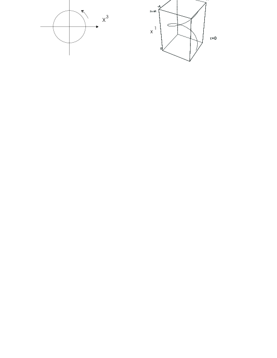
Figure 2: String described by solution (3.22) when $\omega=1$

The velocity modulus is the same for all the points of the string:

$$v=\frac{A\omega}{nR},$$ (3.23)

also in this case there is not a limit for the velocity. From (2.24) and (3.2) we have:

$$E=\frac{J^{2}}{2TA^{2}\pi nR}.$$ (3.24)

For this solution the inertial momentum is $TA^{2}\pi nR$ and is bigger than that one of the solution (3.3). This is in agreement with the classical intuition because now the string is on an average more distant from the rotation axis.

For this solution the momenta along the string is given by

$${\cal P}_{1}=\frac{J^{2}}{2TA^{2}\pi nR}$$ (3.25)

and coincides with the energy of the solution because this configuration verifies the BPS equation and therefore it saturates the BPS bound. We will see that this configuration is ${1\over 4}$ BPS supersymmetric when we embed the bosonic NR string in the NR superstring [7].

Relativistic closed string on spheres with all points moving at the same velocity in modulus, was considered in [10] . They have at least two component of the angular momentum different from zero. However they are different of our NR solutions among other things because they are not supersymmetric.

3.2 Open strings

We now turn to open strings, i.e. solutions of the equations (3.1) satisfying boundary conditions (2). To satisfy the boundary conditions for the longitudinal coordinates we have to fix $K=2nR$ in the static gauge constraints (2.22). We consider a solution with all transverse coordinates satisfying Neumann boundary conditions:

$$x^{0}=2nR\tau\qquad X^{2}=A\cos(\omega\sigma)\sin\left(\omega\tau\right)$$

$$x^{1}=2nR\sigma\qquad X^{3}=A\cos(\omega\sigma)\cos\left(\omega\tau\right).$$ (3.26)

This is an open string with angular momentum perpendicular to the $X^{2}-X^{3}$ plane (figure 3).

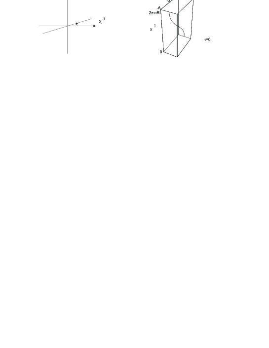
Figure 3: String described by solution (3.26) when $\omega=1$

The string extrema are the faster points and also in this case the velocity modulus $v_{max}=\frac{A\omega}{2nR}$ in not limited. The relation between energy and angular momentum is

$$E=\frac{J^{2}}{TA^{2}\pi nR},$$ (3.27)

i.e. the same relation that we have obtained for the first kind of closed string. For relativistic strings there are different energy-angular momentum relations for open and closed strings.

4 Classical Solutions for NR strings in curved space time

We now analyze the dynamics of strings propagating in a curved transverse space. Since the transverse metric should be Ricci flat in order to have a consistent NR string at quantum level, here we consider the case of a singular conifold with metric $ds^{2}=dr^{2}+r^{2}ds^{2}_{T^{1,1}}$. The $T^{1,1}$ is the conifold base, i.e. the 5-dimensional space $T^{1,1}$[8],

$$ds^{2}_{(T^{1,1})}=\qquad\qquad\qquad\qquad\qquad\qquad$$

$$=\left(\frac{1}{9}(d\psi+\cos\theta_{1}d\phi_{1}+\cos\theta_{2}d\phi_{2})^{2}+\frac{1}{6}(d\theta_{1}^{2}+\sin^{2}\theta_{1}d\phi_{1}^{2}+d\theta_{1}^{2}+\sin^{2}\theta_{2}d\phi_{2}^{2})\right)\qquad$$ (4.1)

where the coordinates $X^{a}$ are renamed $r,\psi$, $\phi_{1}$, $\phi_{2}$, $\theta_{1}$, $\theta_{2}$. This metric does not depend on $\psi$, $\phi_{1}$, $\phi_{2}$ and the action is invariant under translations of these angles. The conserved quantities associated to these symmetries are the angular momenta:

$$J_{i}=\int^{2\pi}_{0}d\sigma P_{\hat{a}}=T\int^{2\pi}_{0}d\sigma\dot{X^{\hat{b}}}G_{\hat{a}\hat{b}}^{(T^{1,1})}\qquad\hat{a},\hat{b}=1,2,3$$

$$\qquad(X^{1}=\psi\qquad X^{2}=\phi_{1}\qquad X^{3}=\phi_{2})\qquad$$ (4.2)

We now consider solutions of the equations of motion (2.17) describing closed strings, i.e. solutions satisfying the boundary conditions (2.20).

4.1 Point like strings

We write three different solutions describing strings that in the transverse space are point particle periodically moving. Considering also the longitudinal part, these are circular extended strings. For these solutions the energy is obtained by (2.24) and the angular momentum by (4). All of them have $r=C$, where $C$ is a constant:

• One $\tau$-dependent transverse coordinate:

  $$x^{0}=nR\tau\qquad x^{1}=nR\sigma\qquad\psi=\nu nR\tau\qquad\phi_{1}=\phi_{2}=\theta_{1}=\theta_{2}=0\qquad$$ (4.3)

  $$J_{\psi}=J_{\phi_{1}}=J_{\phi_{2}}=TnR2\pi\nu\frac{C^{2}}{9}\qquad\qquad E=nRT\pi\nu^{2}\frac{C^{2}}{9}$$ (4.4)

• Two $\tau$-dependent transverse coordinates:

  $$x^{0}=nR\tau\qquad x^{1}=nR\sigma\qquad\psi=\phi_{1}=\nu nR\tau\qquad\theta_{1}=\theta_{2}=\phi_{2}=0\qquad$$ (4.5)

  $$J_{\psi}=J_{\phi_{1}}=J_{\phi_{2}}=TnR2\pi\nu\frac{2}{9}C^{2}\qquad\qquad E=nRT\pi\nu^{2}\frac{4}{9}C^{2}$$ (4.6)

• Three $\tau$-dependent transverse coordinates:

  $$x^{0}=nR\tau\qquad x^{1}=nR\sigma\qquad\psi=\phi_{1}=\phi_{2}=\nu nR\tau\qquad\theta_{1}=\theta_{2}=0\qquad$$ (4.7)

  $$J_{\psi}=J_{\phi_{1}}=J_{\phi_{2}}=TnR2\pi\nu\frac{C^{2}}{3}\qquad\qquad E=nRT\pi\nu^{2}C^{2}$$ (4.8)

For the three point like solutions, the relation between energy and angular momentum is the same, i.e.:

$$E=3\frac{J_{\psi}^{2}}{4\pi nRTC^{2}}+3\frac{J_{\phi_{1}}^{2}}{4\pi nRTC^{2}}+3\frac{J_{\phi_{2}}^{2}}{4\pi nRTC^{2}}.$$ (4.9)

For all these point like solutions the momenta ${\cal P}_{1}=0$.

4.2 Extended string

We now consider a string that is extended also in the transverse space and like (3.22) is moving along its own extension:

$$x^{0}=nR\tau\qquad x^{1}=nR\sigma\qquad\phi_{1}=\nu nR\tau-\omega\sigma\qquad\psi=\phi_{2}=\theta_{1}=\theta_{2}=0\qquad$$ (4.10)

where $\omega\in\mathbb{N}$. This is a closed string because $\phi_{1}\in(0,2\pi)$.

¿From (4) we obtain:

$$J_{\psi}=J_{\phi_{1}}=J_{\phi_{2}}=TnR2\pi\nu\frac{C^{2}}{9}.$$ (4.11)

Using (2.24) we have:

$$E=nRT\pi\nu^{2}\frac{C^{2}}{9}+\pi\frac{C^{2}}{9}\frac{T}{nR}\omega^{2}$$ (4.12)

and finally we find

$$E=3\frac{J_{\psi}^{2}}{4\pi nRTC^{2}}+3\frac{J_{\phi_{1}}^{2}}{4\pi nRTC^{2}}+3\frac{J_{\phi_{2}}^{2}}{4\pi nRTC^{2}}+\pi\frac{C^{2}}{9}\frac{T}{nR}\omega^{2}.\qquad$$ (4.13)

For this solution

$${\cal P}_{1}=T\nu\omega 2\pi\frac{C^{2}}{9}.$$ (4.14)

The BPS equation (2.27) is satisfied when $\nu=\frac{\omega}{nR}$; in fact, in this case from (4.12) and (4.14) we have $E={\cal P}_{1}$.

5 Supersymmetry properties of the solutions

In [7] it has been considered a supersymmetric extension of the bosonic string (2.4) in flat space time. The NR superstring has diffeomorphism and kappa invariance in 10 dimensions. The action in the static gauge and with half of the fermions set to zero has the following form

$$S=-T\;\int d^{2}\sigma\left[\frac{1}{2}\;\eta^{ij}\partial_{i}X\cdot\partial_{j}X\;+\;2i\;{\overline{\theta}}_{+}\Gamma^{i}\partial_{i}\theta_{+}\right]$$ (5.1)

where $\theta_{+}$ is a $+1$ eigenspinor of $\Gamma_{*}=\Gamma_{0}\Gamma_{1}\Gamma_{11}$ with 16 components and $\bar{\theta}_{+}$ is the conjugate spinor. Note that this lagrangian is quadratic in the bosonic and fermionic variables.

The action (5.1) is invariant under the supersymmetry transformations

$$\delta\theta_{+}=\epsilon_{+}\;+\;\frac{1}{2}\Gamma_{\mu}\partial_{i}x^{\mu}\partial^{i}X^{a}\Gamma_{a}\epsilon_{-},\quad\quad\delta X^{a}\;=\;2i{\overline{\theta}}_{+}\Gamma^{a}\epsilon_{-}$$ (5.2)

where $\epsilon_{+}$ and $\epsilon_{-}$ are 16 components constant spinors.

The bosonic supersymmetric configurations of the action (5.1) should verify

$$\epsilon_{+}\;=\;-\frac{1}{2}\Gamma_{\mu}\partial_{i}x^{\mu}\partial^{i}x^{a}\Gamma_{a}\epsilon_{-},$$ (5.3)

with $\epsilon_{\pm}$ constants spinors. When this relation is verified for some non-vanishing components of $\epsilon_{\pm}$ the configuration preserves some of the 32 supersymmetries of the action (5.1).

The vacuum configuration of the string

$$x^{0}=K\tau,\quad\quad x^{1}=K\sigma,\quad\quad\;X^{a}={\rm constant}$$ (5.4)

is supersymmetric if $\epsilon_{+}\;=\;0$ which implies

$$\Gamma^{0}\Gamma^{1}\Gamma_{11}\epsilon=\epsilon.$$ (5.5)

Therefore the string is a $\frac{1}{2}$ BPS configuration. Note that the vacuum solution (5.4) is a solution of both the relativistic and NR string.

There are other possible bosonic supersymmetric configurations with non-constant transverse coordinates. If we write $X^{a}=X^{a}(\tau,\sigma)$, we can have a solution of (5.3) if

$$\partial_{\tau}X^{b}=\pm\partial_{\sigma}X^{b},\quad\quad{\rm and}\quad\quad\Gamma_{0}\epsilon_{-}=\pm\Gamma_{1}\epsilon_{-}.$$ (5.6)

Together with the condition $\epsilon_{+}=0$ the susy parameter $\epsilon$ should satisfy

$$\mp\Gamma^{0}\Gamma^{1}\epsilon=\epsilon.$$ (5.7)

This configuration is a ${1\over 4}$ BPS configuration. It represents a wave propagating, with the velocity of light, along a string with arbitrary profile in the transverse directions.

The supersymmetric (BPS) condition (5.6) was obtained previously as a condition to saturate the energy bound (2.26).

Now we can study the symmetry properties of the solutions we have found. The solutions (3.3) and (3.6) are not supersymmetric because the condition (5.3) can not be verified. Instead the solution (3.1) verifies the supersymmetry condition if the spinors verify $\epsilon_{+}\;=\;0$ and $\Gamma_{0}\epsilon_{-}=\pm\Gamma_{1}\epsilon_{-}$. It is therefore a ${1\over 4}$ BPS configuration. For the solutions in flat space time that we have considered, we observe that if the BPS energy bound (2.26) is verified the solution is supersymmetric.

In the case of a transverse curved manifold there is not yet a general discussion about the supersymmetry properties of a NR superstring in these backgrounds. Therefore for the solutions we have found in transverse curved background we make the ansatz that the solutions that saturate the energy bound (2.26) will be supersymmetric.

6 Conclusions

In this paper we have considered NR string theory in curved transverse space. Our starting point has been the Nambu-Goto action for NR strings in a curved transverse space (2.4). We have then rewritten the action in a Polyakov like form (2.11) and we have derived a BPS bound for the energy in the static gauge.

We have seen that the theory is conformal at quantum level if the transverse space is Ricci flat. For this reason we have considered the case of a singular conifold [8].

We also have found classical rotating solutions of NR strings. The solutions have typical features of a non relativistic theory. In particular, the velocity of the strings has not any limit (3.4),(3.7),(3.23) and the energy is proportional to squared angular momentum (3.5),(3.8),(3.24),(3.27),(4.9),(4.13).

For the flat space case, the BPS equation is obtained as condition to saturate the energy bound (2.27) or as a supersymmetry condition (5.6).

Some of the solutions are ${1\over 4}$ BPS supersymmetric and represent a wave with the velocity of light propagating along the string.

These NR string have a energy spectrum of non-relativistic theories but keep relativistic properties along the longitudinal directions.

7 Acknowledgements

We are grateful to Roberto Emparan, Jaume Gomis, Kiyoshi Kamimura, Tomas Ortín, Josep Maria Pons, Paul Townsend and Toine Van Proeyen for useful discussions and comments. This work is supported in part by the European Community’s Human Potential Programme under contract MRTN-CT-2004-005104 ‘Constituents, fundamental forces and symmetries of the universe’. The work of F.P. is supported in part by the Federal Office for Scientific, Technical and Cultural Affairs through the ”Interuniversity Attraction Poles Programme – Belgian Science Policy” P5/27.

References

• [1] J. Gomis and H. Ooguri, “Non-relativistic closed string theory,” J. Math. Phys.  42 (2001) 3127 [arXiv:hep-th/0009181].
• [2] U. H. Danielsson, A. Guijosa and M. Kruczenski, “IIA/B, wound and wrapped,” JHEP 0010 (2000) 020 [arXiv:hep-th/0009182].
• [3] J. A. Garcia, A. Guijosa and J. D. Vergara, “A membrane action for OM theory,” Nucl. Phys. B 630 (2002) 178 [arXiv:hep-th/0201140].
• [4] J. Brugues, T. Curtright, J. Gomis and L. Mezincescu, “Non-relativistic strings and branes as non-linear realizations of Galilei groups,” Phys. Lett. B 594 (2004) 227 [arXiv:hep-th/0404175].
• [5] E. A. Ivanov and V. I. Ogievetsky, “The Inverse Higgs Phenomenon In Nonlinear Realizations,” Teor. Mat. Fiz.  25 (1975) 164.
• [6] J. P. Gauntlett, J. Gomis and P. K. Townsend, “Particle Actions As Wess-Zumino Terms For Space-Time (Super)Symmetry Groups,” Phys. Lett. B 249 (1990) 255.
• [7] J. Gomis, K. Kamimura and P. K. Townsend, “Non-relativistic superbranes,” arXiv:hep-th/0409219.
• [8] P. Candelas and X. C. de la Ossa, “Comments On Conifolds,” Nucl. Phys. B 342 (1990) 246.
• [9] C. G. . Callan, E. J. Martinec, M. J. Perry and D. Friedan, “Strings In Background Fields,” Nucl. Phys. B 262 (1985) 593.
• [10] J. Hoppe and H. Nicolai, “Relativistic Minimal Surfaces,” Phys. Lett. B 196 (1987) 451.
• [11] M. Kruczenski, “Spiky strings and single trace operators in gauge theories,” arXiv:hep-th/0410226.