UUITP-26/04

hep-th/0411172

Transplanckian energy production
and slow roll inflation

Ulf H. Danielsson

Institutionen för Teoretisk Fysik, Box 803, SE-751 08 Uppsala, Sweden ulf@teorfys.uu.se

Abstract

In this paper we investigate how the energy density due to a non-standard choice of initial vacuum affects the expansion of the universe during inflation. To do this we introduce source terms in the Friedmann equations making sure that we respect the relation between gravity and thermodynamics. We find that the energy production automatically implies a slow rolling cosmological constant. Hence we also conclude that there is no well defined value for the cosmological constant in the presence of sources. We speculate that a non-standard vacuum can provide slow roll inflation on its own.

November 2004

1 Introduction

The main advantage of inflation is that it makes our present day universe to a very large extent insensitive to the precise initial conditions at the Big Bang. In a sense, inflation replaces initial conditions by dynamics and makes a theory of the early universe possible. To be more precise, inflation provides a theory for the effective initial conditions to be imposed on the subsequent evolution of the universe that takes over when inflation ends.

A particular example of this insensitivity to initial conditions, and the resulting predictive power, is the role quantum fluctuations play in the theory of inflation. One of the most amazing suggestions put forward during the past years in cosmology, is that the largest structures of the universe can be traced back, through the expansion of the universe, to microscopical quantum fluctuations occuring during the inflationary era. A natural question to ask, in this context, is how the vacuum for these fluctuations is supposed to be chosen. For inflation to have any predictive power this choice must be highly restricted. Luckily, the key feature of inflation, the accelerated expansion of the universe, provides an answer. If we follow a given fluctuation backwards in time far enough, its wavelength will eventually become arbitrarily smaller than the horizon radius. This means that deviations from Minkowsky space will become less and less important with respect to defining the vacuum, and the vacuum becomes, in this way, essentially unique. This vacuum, sometimes called the Bunch-Davies vacuum, is what one should use when finding out what the predictions of inflation are. The fact that a unique vacuum is picked out is an important property of inflation and is one of several examples of how inflation does away with the need to choose initial conditions.

However, the argument relies on an ability to follow a given mode to infinitely small scales which is not how it is expected to work in the real world. After all, it is generally believed that there exists a fundamental scale – Planckian or stringy – where physics could be completely different from what we are used to, and where we have very little control of what is happening. How does this affect the argument that the inflationary vacuum is unique? Could there be effects of new physics which will affect the predictions of inflation? In particular, could there be appreciable changes in the expected nature of the CMBR fluctuations?

Several groups have investigated ways of modifying high energy physics in order to look for such modifications, see, e.g., [2-25]. One approach is to modify the dispersion relation at high energy – we will come back to a particular toy model of this kind below. Another possible approach, following [7], is to by hand impose initial conditions (in principle coming from unknown high energy physics), corresponding to a particular inflaton quantum state, and to investigate what the effects, if any, there are on the CMBR. To proceed along this direction, we need to find out when to impose the initial conditions for a mode with a given (constant) comoving momentum $k$. To do this, we use conformal time, given by $\tau=-\frac{1}{aH}$, and note that the physical momentum $p$ and the comoving momentum $k$ are related through

$$k=ap=-\frac{p}{\tau H}.$$ (1)

We impose the initial conditions when $p=\Lambda$, where $\Lambda$ is the energy scale, maybe the Planck scale or possibly the string scale, where fundamentally new physics become important. The conformal time when the initial condition is imposed is then given by

$$\tau_{0}=-\frac{\Lambda}{Hk}.$$ (2)

As we see, different modes will be created at different times, with a smaller linear size of the mode (larger $k$) implying a later time.

The basic idea is that we do not know what happens at higher energies, or shorter wavelengths, than $\Lambda,$ and that we therefore are forced to encode our ignorance in terms of initial conditions when the modes enter into the regime that we understand. The unknown high energy physics is usually referred to as transplanckian, and the hope is that, e.g., string theory eventually will give us the means to derive these effective initial conditions. It is well known that the choice of vacuum is a highly non trivial issue in a time dependent background. Without knowledge of the transplanckian physics we can only list various possibilities and investigate whether there is a typical size or signature of the new effects. In [7] an argument was provided for how to choose a natural vacuum and that this vacuum in general can be expected to differ from the Bunch Davies vacuum. Expanding the rescaled inflaton field, $\mu=a\phi$, to lowest adiabatic order as

$$\mu_{k}=\frac{\alpha_{k}}{\sqrt{2k}}e^{-ik\eta}+\frac{\beta_{k}}{\sqrt{2k}}e^{ik\eta},$$ (3)

it was argued in [7] that the Bogolubov coefficients have the natural order

$$\beta\sim\frac{H}{\Lambda}.$$ (4)

As discussed in [9], the initial condition approach to the transplanckian problem allows for a discussion of many of the transplanckian effects in terms of the $\alpha$-vacua. These vacua have been known since a long time, [26], and corresponds to a family of vacua in de Sitter space which respects all the symmetries of the space time. With the use of this input it was shown in [7] how this leads to a simple formula describing a modulated spectrum for the CMBR. Luckily, the possible changes of the standard inflationary predictions are small enough not to ruin the framework, but not so small that they are obviously observationally irrelevant.

One possible concern that one can have with these vacua is in what way the excess energy density that they represent will affect the evolution of the universe. This is the main issue we will investigate in the rest of this paper.

2 The problem of back reaction

The non-standard vacuum contributes an extra energy density that, potentially, could back react on the geometry and change the way the universe expands. Assuming an inflationary cosmology where the inflaton dominates the energy density, we must make sure that the contribution from the vacuum energy is negligible [27]. The energy density is given by

$$\rho_{\Lambda}\sim\int_{0}^{\Lambda}dpp^{3}\left|\beta\right|^{2}\sim\Lambda^{2}\left|\beta\right|^{2},$$ (5)

assuming scale independent Bogolubov coefficients, where we have assumed that there is no contribution to the energy density above the fundamental scale $\Lambda$. This energy density needs to be compared with the energy density driving inflation which is given by

$$\rho\sim M_{pl}^{2}H^{2}.$$ (6)

If one wants to avoid the excess vacuum energy to affect the expansion rate of the universe, one must make sure that $\rho_{\Lambda}\ll\rho$. Luckily, this is the case for the vacua argued to be natural in [7]. From above it follows that we can ignore the effect of the vacuum energy provided that $\Lambda\ll M_{pl}$, which has to be assumed in these models for other reasons. Furthermore, with $\Lambda$ as the string scale, this is a rather natural requirement. However, as we will see further on, there is more to the story than this, and we will find that the vacuum energy can play a quite important role under the right circumstances.

Another objection was put forward in [28], where it was argued that the same physics selecting a non standard vacuum during inflation should still be at work today. The value of $\beta$ would certainly be expected to be much smaller, presumably determined by the present day Hubble constant, and the expected energy density would be $\rho\sim\Lambda^{2}H_{today}^{2}$. Nevertheless, one would expect this energy to be present in the form of ultra high energy particles which, through their interactions with other matter, would produce also lower energy gamma and cosmic rays. The estimated rates are a few order of magnitude higher than what is measured, and in [28] this was used to argue for limits on the possible vacua such that effects on the CMBR are excluded.

In [25] it was proposed that even a substantial energy density arising from vacuum fluctuations (not necessarily with the value of $\beta$ used in this paper) might not destroy inflation but instead act like a renormalization of the inflationary cosmological constant. This was shown in the framework of a particular transplanckian model with a modified dispersion relation. The focus in this model is on a scalar field with a modified dispersion relation at high energies, see figure 1.

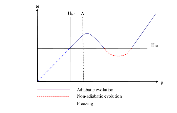
Figure 1: The evolution (not to scale) of a mode with a modified dispersion relation during inflation. The effective initial conditions imposed at $p=\Lambda$ will be the ones of an excited state.

At low energies the dispersion relation is linear with frequency increasing with momentum in the standard fashion. In an intermediate energy range the frequency decreases with momentum, and then at high energies it increases again. The main idea is that the initial state at really high energies is the adiabatic one. As the universe expands, and the energy redshifts, the frequency of a mode remains, for high energies, larger than the Hubble constant. This corresponds to an adiabatic evolution and the vacuum does not change. In the intermediate regime the frequency drops due to the non standard dispersion relation. As a consequence it becomes lower than the Hubble constant and the evolution is no longer adiabatic. When the universe has expanded further, and the mode redshifted even more, the frequency again becomes larger than the Hubble constant and another adiabatic phase can begin. At this point, however, the state of the field no longer coincides with the adiabatic vacuum.

Furthermore, in this scenario, it is very natural to expect, contrary to the argument in [28], a very different result for the energy production today. The only thing we need to make sure is that the Hubble scale today is lower than the minimum of the kink on the dispersion relation. This case is shown in figure 2.

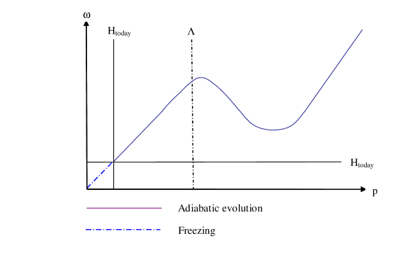
Figure 2: The evolution (not to scale) of a mode with a modified dispersion relation today. The effective initial conditions when $p=\Lambda$ will be the ones of the adiabatic vacuum.

As a consequence, there is no non-adiabatic evolution at transplanckian energies and the vacuum remains the adiabatic one. Hence there is no excessive production of high energy radiation at the present times.In the framework of [7] the new vacuum is used as an initial state once the mode has redshifted out of the regime with a non standard dispersion relation, as is depicted in figure 1. In figure 2 we have a situation where the standard vacuum is picked out.

In the rest of the paper we will show how the same general conclusions about the influence of the extra vacuum energy during inflation, can be reach in the framework of [7] where we do not make any explicit assumptions about the transplanckian physics. It is reassuring though, that a precise example, as the one of [25], exists showing the full consistency of the argument.

3 Sourced Friedmann equations

In order to address the problem of back reaction we will have to introduce the energy density of the non-standard vacuum into the Friedmann equations, and for consistency, we will also need to include a source term due to the continuos creation of modes. From the point of view of the specific model considered in [25] the source would correspond to the non-adiabatic phase where excited modes are created. Contrary to [25], we will, in our simplified framework, be able to solve for the back reaction in some detail. In fact, as will become clear further on, we will see how the vacuum energy can drive inflation all on its own.

In order to generalize the Friedmann equations to include sources, we will find it useful to discuss the equations from the thermodynamical point of view taken in [30].

3.1 A thermodynamical approach to the Friedmann equations

Given the connection between black hole physics and thermodynamics first revealed by Bekenstein in the seventies, [31], it is tempting to speculate about a deeper connection between thermodynamics and gravity in general. Along this line of thought, it was argued in [30] that the gravitational Einstein equations can be derived through a thermodynamical argument using the relation between area and entropy as input. In the simplified cosmological setting relevant for our analysis, the corresponding argument was given in [32].

The starting point is the relation between the area of the horizon and entropy for a black hole given by

$$S=\frac{M_{p}^{2}}{4}A.$$ (7)

In an expanding universe, at least in the case of accelerated expansion, the cosmological horizon determined by the Hubble constant plays a similar role as the horizon of a black hole, [33]. We therefore assign an entropy to the horizon according to

$$S=\frac{\pi M_{p}^{2}}{H^{2}}.$$ (8)

We now proceed with deriving the Friedmann equations describing the time evolution of the universe with the entropy relation as a starting point. To do this, we use the standard relation between flow of heat and entropy, $dQ=TdS$. The flow of heat out through the horizon is then related to a flow of entropy given by

$$\dot{Q}=\dot{S}T=A\left(\rho+p\right),$$ (9)

where

$$T=\frac{H}{2\pi}.$$ (10)

Using that the entropy can be expressed in terms of the horizon area and the Hubble constant, we find

$$\dot{H}=-\frac{4\pi}{M_{p}^{2}}\left(\rho+p\right),$$ (11)

which, indeed, is one of the Friedmann equations.

To completely specify the time evolution we also need the continuity equation

$$\overset{\cdot}{\rho}+3H\left(\rho+p\right)=0,$$ (12)

which, combined with (11), give another of the Friedmann equations, i.e.,

$$H^{2}=\frac{8\pi}{3M_{p}^{2}}\rho.$$ (13)

Usually the two Friedmann equations together with the continuum equation are viewed on an equal footing keeping in mind that only two of them are independent. However, from our thermodynamical point of view, there is an important difference between the various choices. (13) is obtained from (11) using integration and there is, therefore, a corresponding constant of integration, the cosmological constant, which does not appear in the basic equations (11). The usual interpretation is that the cosmological constant corresponds to matter with $p=-\rho$. However, from our thermodynamical point of view, it is more natural to view the cosmological constant as part of the initial conditions.

While the above argument was carried out for the specific example of a FRW-cosmology, it was given in all generality in [30], where it was shown that the thermodynamical approach to gravity required

$$8\pi GT_{\mu\nu}=R_{\mu\nu}+fg_{\mu\nu},$$ (14)

with $f$ an arbitrary function. If one then demands that the energy momentum tensor is conserved, one finds that $f=-\frac{R}{2}+\Lambda_{c}$ with $\Lambda_{c}$ as the cosmological constant, and the Einstein equations follows.

The thermodynamical approach to gravity might be considered as a curious observation, and nothing more. In the following we will see, however, that this point of view makes it a bit easier to think about an expanding universe in the presence of sources.

3.2 With sources

How does the above derivation of the Friedmann equations change if $T_{\mu\nu}$ is not conserved? From a thermodynamical point of view it is obvious that we should make sure that we keep (11) unchanged. This is the equation that relates the change in area of the horizon with the local flow of matter and energy, and is required by the thermodynamical interpretation of horizon area. On the other hand, we have, in the presence of a source $q$,

$$\overset{\cdot}{\rho}+3H\left(\rho+p\right)=q,$$ (15)

which is easily seen to lead to

$$H^{2}=\frac{8\pi}{3M_{p}^{2}}\rho-\frac{8\pi}{3M_{p}^{2}}\int^{t}qdt.$$ (16)

It is clear that (11) should remain the same even in the presence of sources, but we see that this is not at all true for (13).

While we will not need this in the present paper, it is trivial to perform a general analysis for other backgrounds. We write the generalized continuity equation and Einstein equation as

$$8\pi G\nabla^{\mu}T_{\mu\nu} =g_{\mu\nu}\nabla^{\mu}h$$ (17)

$$8\pi GT_{\mu\nu} =G_{\mu\nu}+hg_{\mu\nu}.$$ (18)

With the energy momentum tensor on the form

$$T_{\mu\nu}=\left(\rho+p\right)V_{\mu}V_{\nu}-pg_{\mu\nu},$$ (19)

it is easy to see that we can define a new energy momentum tensor that is conserved, with new energy and pressure given by

$$\tilde{\rho} =\rho+h$$ (20)

$$\tilde{p} =p-h$$ (21)

In our cosmological example we have

$$\tilde{\rho}=\rho-\int^{t}qdt$$ (22)

After this general discussion, let us turn to the transplanckian problem.

4 The effect of transplanckian energy production

4.1 General discussion

Let us now make use of the results of the previous section. In addition to the non-standard vacuum, we allow for the existence of ordinary matter. The two contributions obey the continuity equations

$$\overset{\cdot}{\rho}_{\Lambda}+3H\left(\rho_{\Lambda}+p_{\Lambda}\right) =q$$ (23)

$$\overset{\cdot}{\rho}_{m}+3H\left(\rho_{m}+p_{m}\right) =0,$$ (24)

where we have allowed for energy production in the vacuum sector, and we have assumed that all other matter obey the standard equations. We assume the equations of state to be given by

$$p_{\Lambda} =w_{\Lambda}\rho_{\Lambda}$$ (25)

$$p_{m} =w_{m}\rho_{m},$$ (26)

We then impose the Friedmann equation

$$\dot{H}=-\frac{4\pi}{M_{p}^{2}}\left(\rho_{\Lambda}+p_{\Lambda}+\rho_{m}+p_{m}\right),$$ (27)

where we will put $w_{\Lambda}=\frac{1}{3}$, and keep $w_{m}$ arbitrary. Integrating the equations gives

$$H^{2}=\frac{8\pi}{3M_{p}^{2}}\left(\rho_{\Lambda}+\rho_{m}\right)-\frac{8\pi}{3M_{p}^{2}}\int^{t}qdt,$$ (28)

as discussed in the previous section.

Let us now consider the specific case of vacuum fluctuations with the characteristic values of the Bogolubov mixing given by

$$\left|\beta_{k}\right|^{2}\sim\frac{H^{2}}{\Lambda^{2}}.$$ (29)

Assuming an essentially constant $H$, and integrating over all energies up to the cutoff scale yields

$$\rho_{\Lambda}\sim\int_{0}^{\Lambda}dpp^{3}\frac{H^{2}}{\Lambda^{2}}\sim\Lambda^{2}H^{2}.$$ (30)

For convenience we redefine $\Lambda$ such that

$$\rho_{\Lambda}=\frac{3\Lambda^{2}H^{2}}{8\pi}.$$ (31)

Actually, we will have to be a bit more careful than this. Since $H$ will be changing with time, i.e. decrease, we must take this into account when calculating the vacuum energy density. Modes with low momenta were created at earlier times when the value of $H$ were larger, and there will be a slight enhancement in the way these modes contribute to the energy density. We therefore write

$$\rho_{\Lambda}\left(a\right)=\frac{3}{2\pi}\int_{\varepsilon}^{\Lambda}dpp^{3}\frac{H^{2}\left(\frac{ap}{\Lambda}\right)}{\Lambda^{2}}=\frac{3}{2\pi}\frac{1}{\Lambda^{2}a^{4}}\int_{a_{i}}^{a}dxx^{3}H^{2}\left(x\right),$$ (32)

where we have introduced a low energy cutoff corresponding to the present energy of modes that started out at $\Lambda$ at a time when the Hubble constant was as small as $H_{i}$.

If we take a derivative of the energy density with respect to the scale factor and use $\frac{d}{da}=\frac{1}{aH}\frac{d}{dt}$, we find

$$\dot{\rho}_{\Lambda}+4H\rho_{\Lambda}=\frac{3}{2\pi}\Lambda^{2}H^{3},$$ (33)

and we can conclude that the source term is given by

$$q=\frac{3}{2\pi}\Lambda^{2}H^{3}.$$ (34)

To proceed it is convenient to write (33) in the form

$$\frac{d}{da}\left(a^{4}\rho_{\Lambda}\right)=\frac{3}{2\pi}\Lambda^{2}a^{3}H^{2},$$ (35)

and take a derivative of (27) with respect to the scale factor to obtain

$$a^{2}HH^{\prime\prime}+a^{2}H^{\prime 2}+5aHH^{\prime}=-\frac{8\Lambda^{2}}{M_{p}^{2}}H^{2}-\frac{4\pi}{M_{p}^{2}}\left(1+w_{m}\right)\left(1-3w_{m}\right)\rho_{m},$$ (36)

where we have used that $\rho_{m}\sim a^{-3\left(1+w_{m}\right)}$. The general solution is easily found to be

$$H^{2}=C_{1}^{2}a^{-2n_{1}}+C_{2}^{2}a^{-2n_{2}}+\frac{8\pi}{3M_{p}^{2}}\frac{\left(1+w_{m}\right)\left(1-3w_{m}\right)}{\left(1+w_{m}\right)\left(1-3w_{m}\right)-\frac{16\Lambda^{2}}{3M_{p}^{2}}}\rho_{m},$$ (37)

where $C_{1,2}$ are constants of integration, and

$$n_{1,2}=1\pm\sqrt{1-\frac{4\Lambda^{2}}{M_{p}^{2}}}.$$ (38)

In the limit $\Lambda\rightarrow 0$ (implying that the vacuum energy is removed) we find

$$H^{2}=C_{1}^{2}+C_{2}^{2}a^{-4}+\frac{8\pi}{3M_{p}^{2}}\rho_{m}.$$ (39)

That is, $C_{1}$ gives a cosmological constant, while $C_{2}$ corresponds to radiation, both of which can be absorbed into $\rho_{m}$. More interesting, is the case when $\Lambda\neq 0$. We see, then, that neither a cosmological constant nor, which is less expected, a radiation component survives in (37) since $\left(1+w_{m}\right)\left(1-3w_{m}\right)=0$ for $w_{m}=-1$ or $w_{m}=1/3$. Instead, they both appear through constants of integration. Furthermore, due to the source term, the way the two components depend on the scale factor is changed. For small $\frac{\Lambda^{2}}{M_{p}^{2}}$, we find

$$\left\{\begin{array}[c]{l}n_{1}\sim 2-\frac{2\Lambda^{2}}{M_{p}^{2}}\\ n_{2}\sim\frac{2\Lambda^{2}}{M_{p}^{2}}.\end{array}\right.$$ (40)

The first corresponds to a radiation component which is decaying with redshift a bit slower than usual, while the other is more like a cosmological constant that is slowly decreasing.

Let us finally consider the case with only radiation, that is $w_{m}=1/3$, in some more detail. We then have

$$H^{2}=C_{1}^{2}a^{-2n_{1}}+C_{2}^{2}a^{-2n_{2}}$$ (41)

In particular, let us consider the initial moment when $H=H_{i}$. At that time we have, by definition, $\rho_{\Lambda}=0$. Note that $\rho_{\Lambda}$ always correspond to energy created after the time of an, arbitrary, initial scale factor $a_{i}$. But how much radiation is already present? This is given directly by (27), since the flow of radiation out through the horizon dictates the way the Hubble constant changes. We find

$$\frac{a}{2}\frac{d}{da}H^{2}=-\frac{16\pi}{3M_{p}^{2}}\rho_{m},$$ (42)

from which we conclude

$$\frac{8\pi}{3M_{p}^{2}}\rho_{m}=\frac{n_{1}}{2}C_{1}^{2}a_{i}^{-2n_{1}}+\frac{n_{2}}{2}C_{2}^{2}a_{i}^{-2n_{2}}.$$ (43)

That is, for any $a_{i}$, we can read off the amount of radiation present at that scale factor. It is not very surprising that the evolution with the scale factor does not go as $1/a^{4}$, since, after all, we have made sure that there is a continuos creation of matter. It is interesting to consider the difference between (41) and (43). This is given by

$$\frac{8\pi}{3M_{p}^{2}}\rho_{\Lambda_{cc}}=C_{1}^{2}\left(1-\frac{n_{1}}{2}\right)a^{-2n_{1}}+C_{2}^{2}\left(1-\frac{n_{2}}{2}\right)a^{-2n_{2}},$$ (44)

and would be expected to be identified with a cosmological constant. This is, however, true only in the limits where $\Lambda=0$. Otherwise we obtain a cosmological constant that is slowly decaying. It is important to observe that in the presence of sources one can not assign an unambiguous value to the cosmological constant. This is one of the main conclusions of the paper. We find that a fixed dimensionful cosmological constant, is effectively replaced by a dimensionless parameter determining the running, given by the ratio of a fundamental scale and the Planck scale.

5 Conclusions and speculations

In this paper we have investigated in what way a non-standard vacuum affects the expansion of the universe during inflation due to the extra energy density. To do this we have found it necessary to include a source term in the continuity equation that also affected one of the Friedmann equations. A nice framework for understanding how to make the appropriate modifications is provided by the work of [30].

We have found, in the presence of sources (e.g. due to non-adiabatic transplanckian physics), that a cosmological constant is replaced by a running quantity. These results are consistent with, and generalize, what was found in [25]. As a consequence, a non-standard vacuum can yield an inflationary slowroll all on its own even with out a nontrivial inflationary potential. The results suggests that in searching for phenomenologically viable inflationary models, the choice of initial vacuum (or equivalently, the details of transplanckian physics) could play a similar role as the shape of the inflaton potential. It would be interesting to find models with more detailed phenomenology and also investigate the relation with detectable modulations of the CMBR. This is left for future work.

References

- [1] A. R. Liddle and D. H. Lyth, “Cosmological inflation and large-scale structure”, Cambridge University Press 2000.
- [2] R. H. Brandenberger, “Inflationary cosmology: Progress and problems,” arXiv:hep-ph/9910410. J. Martin and R. H. Brandenberger, “The trans-Planckian problem of inflationary cosmology,” Phys. Rev. D 63, 123501 (2001) [arXiv:hep-th/0005209].
- [3] A. A. Starobinsky, “Robustness of the inflationary perturbation spectrum to trans-Planckian physics,” Pisma Zh. Eksp. Teor. Fiz. 73, 415 (2001) [JETP Lett. 73, 371 (2001)] [arXiv:astro-ph/0104043].
- [4] R. Easther, B. R. Greene, W. H. Kinney and G. Shiu, “Inflation as a probe of short distance physics,” Phys. Rev. D 64, 103502 (2001) [arXiv:hep-th/0104102]. “Imprints of short distance physics on inflationary cosmology,” Phys. Rev. D 67 (2003) 063508 [arXiv:hep-th/0110226]. “A generic estimate of trans-Planckian modifications to the primordial power Phys. Rev. D 66 (2002) 023518 [arXiv:hep-th/0204129].
- [5] N. Kaloper, M. Kleban, A. E. Lawrence and S. Shenker, Phys. Rev. D 66 (2002) 123510 [arXiv:hep-th/0201158].
- [6] S. Shankaranarayanan, “Is there an imprint of Planck scale physics on inflationary cosmology?,” Class. Quant. Grav. 20, 75 (2003) [arXiv:gr-qc/0203060].
- [7] U. H. Danielsson, “A note on inflation and transplanckian physics,” Phys. Rev. D 66, 023511 (2002) [arXiv:hep-th/0203198].
- [8] S. F. Hassan and M. S. Sloth, “Trans-Planckian effects in inflationary cosmology and the modified uncertainty principle,” Nucl. Phys. B 674 (2003) 434 [arXiv:hep-th/0204110].
- [9] U. H. Danielsson, “Inflation, holography and the choice of vacuum in de Sitter space,” JHEP 0207, 040 (2002) [arXiv:hep-th/0205227].
- [10] J. C. Niemeyer, R. Parentani and D. Campo, “Minimal modifications of the primordial power spectrum from an adiabatic Phys. Rev. D 66 (2002) 083510 [arXiv:hep-th/0206149].
- [11] K. Goldstein and D. A. Lowe, “Initial state effects on the cosmic microwave background and trans-planckian Phys. Rev. D 67 (2003) 063502 [arXiv:hep-th/0208167].
- [12] U. H. Danielsson, “On the consistency of de Sitter vacua,” JHEP 0212 (2002) 025 [arXiv:hep-th/0210058].
- [13] C. P. Burgess, J. M. Cline, F. Lemieux and R. Holman, “Are inflationary predictions sensitive to very high energy physics?,” JHEP 0302 (2003) 048 [arXiv:hep-th/0210233].
- [14] L. Bergström and U. H. Danielsson, “Can MAP and Planck map Planck physics?,” JHEP 0212 (2002) 038 [arXiv:hep-th/0211006].
- [15] J. Martin and R. Brandenberger, “On the dependence of the spectra of fluctuations in inflationary cosmology Phys. Rev. D 68 (2003) 063513 [arXiv:hep-th/0305161].
- [16] O. Elgaroy and S. Hannestad, “Can Planck-scale physics be seen in the cosmic microwave background?,” Phys. Rev. D 68 (2003) 123513 [arXiv:astro-ph/0307011].
- [17] J. Martin and C. Ringeval, “Superimposed Oscillations in the WMAP Data?,” Phys. Rev. D 69 (2004) 083515 [arXiv:astro-ph/0310382].
- [18] T. Okamoto and E. A. Lim, “Constraining Cut-off Physics in the Cosmic Microwave Background,” Phys. Rev. D 69 (2004) 083519 [arXiv:astro-ph/0312284].
- [19] K. Schalm, G. Shiu and J. P. van der Schaar, “Decoupling in an expanding universe: Boundary RG-flow affects initial JHEP 0404 (2004) 076 [arXiv:hep-th/0401164].
- [20] J. de Boer, V. Jejjala and D. Minic, “Alpha-states in de Sitter space,” arXiv:hep-th/0406217.
- [21] V. Bozza, M. Giovannini and G. Veneziano, “Cosmological perturbations from a new-physics hypersurface,” JCAP 0305 (2003) 001 [arXiv:hep-th/0302184].
- [22] C. P. Burgess, J. M. Cline and R. Holman, “Effective field theories and inflation,” JCAP 0310 (2003) 004 [arXiv:hep-th/0306079].
- [23] U. H. Danielsson and M. E. Olsson, “On thermalization in de Sitter space,” JHEP 0403 (2004) 036 [arXiv:hep-th/0309163].
- [24] T. Banks and L. Mannelli, “De Sitter vacua, renormalization and locality,” Phys. Rev. D 67 (2003) 065009 [arXiv:hep-th/0209113]. M. B. Einhorn and F. Larsen, Phys. Rev. D 67 (2003) 024001 [arXiv:hep-th/0209159]. M. B. Einhorn and F. Larsen, “Squeezed states in the de Sitter vacuum,” Phys. Rev. D 68 (2003) 064002 [arXiv:hep-th/0305056]. N. Kaloper, M. Kleban, A. Lawrence, S. Shenker and L. Susskind, “Initial conditions for inflation,” JHEP 0211 (2002) 037 [arXiv:hep-th/0209231].
- [25] R. H. Brandenberger and J. Martin, “Back-reaction and the trans-Planckian problem of inflation revisited,” arXiv:hep-th/0410223.
- [26] N. A. Chernikov and E. A. Tagirov, “Quantum theory of scalar field in de Sitter space-time,” Ann. Inst. Henri Poincaré, vol. IX, nr 2, (1968) 109. E. Mottola, “Particle Creation In De Sitter Space,” Phys. Rev. D 31 (1985) 754. B. Allen, “Vacuum States In De Sitter Space,” Phys. Rev. D 32 (1985) 3136. R. Floreanini, C. T. Hill and R. Jackiw, “Functional Representation For The Isometries Of De Sitter Space,” Annals Phys. 175 (1987) 345. R. Bousso, A. Maloney and A. Strominger, “Conformal vacua and entropy in de Sitter space,” arXiv:hep-th/0112218. M. Spradlin and A. Volovich, “Vacuum states and the S-matrix in dS/CFT,” arXiv:hep-th/0112223.
- [27] T. Tanaka, “A comment on trans-Planckian physics in inflationary universe,” arXiv:astro-ph/0012431.
- [28] A. A. Starobinsky and I. I. Tkachev, “Trans-Planckian particle creation in cosmology and ultra-high energy cosmic JETP Lett. 76 (2002) 235 [Pisma Zh. Eksp. Teor. Fiz. 76 (2002) 291] [arXiv:astro-ph/0207572].
- [29] E. Keski-Vakkuri and M. S. Sloth, “Holographic bounds on the UV cutoff scale in inflationary cosmology,” JCAP 0308 (2003) 001 [arXiv:hep-th/0306070].
- [30] T. Jacobson, “Thermodynamics of space-time: The Einstein equation of state,” Phys. Rev. Lett. 75 (1995) 1260 [arXiv:gr-qc/9504004].
- [31] J. D. Bekenstein, “Generalized Second Law Of Thermodynamics In Black Hole Physics,” Phys. Rev. D 9, 3292 (1974).
- [32] A. V. Frolov and L. Kofman, “Inflation and de Sitter thermodynamics,” JCAP 0305 (2003) 009 [arXiv:hep-th/0212327].
- [33] G. W. Gibbons, S. W. Hawking, “Cosmological event horizons, thermodynamics, and particle creation,” Phys. Rev. D 15 (1977) 2738.
- [34] R. Horvat, “Holography and variable cosmological constant,” Phys. Rev. D 70 (2004) 087301 [arXiv:astro-ph/0404204].
- [35] E. Mottola, “Particle Creation In De Sitter Space,” Phys. Rev. 31 (1985) 754.