Abstract

We construct infinitely many seven-dimensional Einstein metrics of weak holonomy $G_{2}$. These metrics are defined on principal SO(3) bundles over four-dimensional Bianchi IX orbifolds with the Tod-Hitchin metrics. The Tod-Hitchin metric has an orbifold singularity parameterized by an integer, and is shown to be similar near the singularity to the Taub-NUT de Sitter metric with a special charge. We show, however, that the seven-dimensional metrics on the total space are actually smooth. The geodesics on the weak $G_{2}$ manifolds are discussed. It is shown that the geodesic equation is equivalent to the Hamiltonian equation of an interacting rigid body system. We also discuss M-theory on the product space of AdS₄ and the seven-dimensional manifolds, and the dual gauge theories in three-dimensions.

1 Introduction

M-theory compactifications on special holonomy manifolds have attracted much attention, because they preserve some supersymmetry and allow to examine dynamical aspects of a large class of supersymmetric gauge theories [1]. For example, it is known that there are eight-dimensional Ricci flat manifolds with holonomy Sp(2), SU(4) and Spin(7) except for the trivial one, and M-theory compactifications on them correspond to three-dimensional gauge theories with ${\mathcal{N}}=3$, $2$ and $1$ supersymmetry, respectively. For a non-compact eight-dimensional special holonomy manifold, M-theory on it is interpreted as a worldvolume theory on an M2-brane with a special holonomy manifold as the transverse space. This is closely related to the supersymmetric M-theory solution AdS${}_{4}\times M$ with compact seven-dimensional Einstein manifold $M$. For weak $G_{2}$ manifolds $M$, namely, 3-Sasakian, Sasaki-Einstein and proper weak $G_{2}$ manifolds, the M-theory solutions AdS${}_{4}\times M$ are AdS/CFT dual to ${\mathcal{N}}=3$, $2$ and $1$ superconformal field theories on the boundary of AdS₄ [2][3][4][5]. The brane solution naturally interpolates between AdS${}_{4}\times M$ in the near horizon limit and ${\mathbb{R}}^{1,2}\times C(M)$, where $C(M)$ is the cone over $M$ with the special holonomy SP(2), SU(4) or Spin(7), and the gauge theories on the both sides are related by the RG-flow [6].

In this paper, we construct infinitely many seven-dimensional Einstein metrics admitting 3-Sasakian and proper weak $G_{2}$ structures . These metrics are defined on compact manifolds $M_{k}$ parameterized by an integer $k\geq 3$; principal SO(3) bundles over four-dimensional Bianchi IX orbifolds with the Tod-Hitchin metrics [9][10][11]. The Tod-Hitchin metric has an orbifold singularity parameterized by the integer $k$. However, the singularity is resolved by adding the fiber SO(3), and so the total spaces $M_{k}$ become smooth manifolds. Our compact manifolds contain manifolds $S^{7}$, $N^{0,1,0}$ and the squashed S⁷ as special homogeneous cases for $k=3,4$ [12]. For generic $k$, the metrics on $M_{k}$ are inhomogeneous and admit SO(3)$\times$SO(3) isometry. This implies that the dual gauge theories in three-dimensions are ${\mathcal{N}}=3$ supersymmetric with SO(3) flavor for 3-Sasakian manifolds $M_{k}$, and ${\mathcal{N}}=1$ supersymmetric with SO(3)$\times$SO(3) flavor for proper weak $G_{2}$ manifolds $M_{k}$. We examine the geodesics on $M_{k}$ using a Hamiltonian formulation on the cotangent bundle $T^{*}M_{k}$. The geodesic equation is equivalent to the Hamiltonian equation of an interacting rigid body system. We find some special solutions, which may be useful to consider the Penrose limit of our metrics.

This paper is organized as follows. In section 2, we introduce the Tod-Hitchin geometry, and explain the relation to the Atiyah-Hitchin manifold [13]. We show that the Tod-Hitchin geometry is well approximated by the Taub-NUT de-Sitter geometry with a special charge. In section 3, we construct infinitely many seven-dimensional Einstein metrics of weak holonomy $G_{2}$ on compact manifolds. We also discuss the geodesics on the weak $G_{2}$ manifolds, in section 4. In the last section, we comment on the M-theory solutions AdS${}_{4}\times M_{k}$ and the dual gauge theories in three-dimensions. In appendix A, we present the anti-self-dual condition for the Bianchi IX Einstein metric. We summarize the relation between the Tod-Hitchin metric and the Painlevé VI solution in appendix B. In appendix C, the $G_{2}$ structure of the metric is given.

2 ASD Einstein metrics on four-dimensional Bianchi IX manifold

In this section, we consider Bianchi IX Einstein metrics with positive cosmological constant. By using the SO(3) left-invariant one-forms $\sigma_{i}$ $(i=1,2,3)$, the metric can be written in the form:

$$g=dt^{2}+a^{2}(t)\sigma_{1}^{2}+b^{2}(t)\sigma_{2}^{2}+c^{2}(t)\sigma_{3}^{2}~{}.$$ (2.1)

In the biaxial case, the general solution to the Einstein equation $Ric(g)=\Lambda g$ has three parameters, the mass $m$, the NUT charge $n$ and the cosmological constant $\Lambda$;

$$g_{\{m,n,\Lambda\}}=\frac{r^{2}-n^{2}}{\Delta(r)}dr^{2}+\frac{4n^{2}\Delta(r)}{r^{2}-n^{2}}\sigma_{1}^{2}+(r^{2}-n^{2})(\sigma_{2}^{2}+\sigma_{3}^{2}),$$ (2.2)

where

$$\Delta(r)=r^{2}-2mr+n^{2}+\Lambda\left(n^{4}+2n^{2}r^{2}-\frac{1}{3}r^{4}\right).$$ (2.3)

The anti-self-dual (ASD) condition for the Weyl curvature determines $m$ in terms of $n$ and $\Lambda$ as

$$m=-n\left(1+\frac{4}{3}\Lambda n^{2}\right),$$ (2.4)

in which case

$$\Delta(r)=\frac{\Lambda}{3}(r+n)^{2}(r_{+}-r)(r-r_{-})~{},~{}~{}~{}r_{\pm}=n\pm\sqrt{4n^{2}+\frac{3}{\Lambda}}~{}.$$ (2.5)

Then the metric (2.2) becomes the ASD Taub-NUT de-Sitter metric [14][15] given by

$$g_{\{n,\Lambda\}}=\frac{dr^{2}}{F(r)}+4n^{2}F(r)\sigma_{1}^{2}+(r^{2}-n^{2})(\sigma_{2}^{2}+\sigma_{3}^{2})~{},$$ (2.6)

where

$$F(r)=\frac{\Lambda}{3}\left(\frac{r+n}{r-n}\right)(r_{+}-r)(r-r_{-})~{}.$$ (2.7)

For $\Lambda=0$, the metric reduces to the ASD Taub-NUT metric [16],

$$g_{\{n,0\}}=\left(\frac{r-n}{r+n}\right)dr^{2}+4n^{2}\left(\frac{r+n}{r-n}\right)\sigma_{1}^{2}+(r^{2}-n^{2})(\sigma_{2}^{2}+\sigma_{3}^{2})~{}.$$ (2.8)

We shall now restrict our attention to the metric (2.6) with the special NUT charge

$$n=\sqrt{\frac{3}{\Lambda(k^{2}-4)}}~{},$$ (2.9)

which is a family of ASD Einstein metrics $g_{k}\equiv g_{\{n=\sqrt{{3}/{\Lambda(k^{2}-4)}},\,\Lambda\}}$ parameterized by the integer $k\geq 3$. Each metric $g_{k}$ has the following properties (see Figure 1):

(a)

When the coordinate $r$ is taken to lie in the interval $n\leq r\leq r_{+}$, the metric has singularities at the boundaries; There is an orbifold singularity at $r=r_{+}$, while a curvature singularity at another boundary $r=n$.

(b)

The metric gives an approximation to the Tod-Hitchin metric.

(c)

As $k\to\infty$ and $\Lambda\to 0$ keeping $\Lambda k^{2}=3$, the metric converges to the ASD Taub-NUT metric (2.8) with a negative mass parameter ($n=1$) which gives the asymptotic form of the Atiyah-Hitchin hyperkähler metric.

Figure 1: The relation among metrics

In the following, we will explain these points in some detail. For this purpose, we start with an explanation of some relevant aspects of the Tod-Hitchin metrics. Tod and Hitchin constructed a family of ASD Einstein metrics (Tod-Hitchin metrics) on the Bianchi IX orbifold, parameterized by an integer $k\geq 3$ [9][10][11]. These solutions are written in the triaxial form and have a compactification as metrics with orbifold singularities. These may be thought of as a resolution of the curvature singularity in the ASD Taub-NUT de-Sitter metric $g_{k}$. Each Tod-Hitchin metric $g^{\rm TH}_{k}$ is given by a solution to the Painlevé VI equation (see appendix B). For lower $k$ the metric takes the form [11][14]:

• $k=3$

  $$g^{\rm TH}_{3}=dt^{2}+4\sin^{2}t~{}\sigma_{1}^{2}+4\sin^{2}(\frac{2}{3}\pi-t)~{}\sigma_{2}^{2}+4\sin^{2}(t+\frac{2}{3}\pi)~{}\sigma_{3}^{2}~{},$$ (2.10)

  which gives the standard metric on S⁴ written in the triaxial form.

• $k=4$

  $$g_{4}^{\rm TH}=dt^{2}+\sin^{2}t~{}\sigma_{1}^{2}+\cos^{2}t~{}\sigma_{2}^{2}+\cos^{2}2t~{}\sigma_{3}^{2}~{},$$ (2.11)

  which gives the Fubini-Study metric on ${\mathbb{CP}}^{2}$.

• $k=6,~{}8$ 
  The metric can be written as

  $$g^{\rm TH}_{k}=h(r)~{}dr^{2}+a^{2}(r)~{}\sigma_{1}^{2}+b^{2}(r)~{}\sigma_{2}^{2}+c^{2}(r)~{}\sigma_{3}^{2}~{},$$ (2.12)

  where the components are given for $k=6$

  $$h^{2}=\frac{3(1+r+r^{2})}{r\,(r+2)^{2}\,(2r+1)^{2}}\,,\qquad a^{2}=\frac{3(1+r+r^{2})}{(r+2)\,(2r+1)^{2}}\,,$$

  $$b^{2}=\frac{3r\,(1+r+r^{2})}{(r+2)^{2}\,(2r+1)}\,,\qquad c^{2}=\frac{3(r^{2}-1)^{2}}{(1+r+r^{2})\,(r+2)\,(2r+1)}~{},$$ (2.13)

  and for $k=8$

  $$h^{2} = \frac{4(1+r)(3-2r+r^{2})(1-2r+3r^{2})(1+2r+3r^{2})}{(1-r)\,r\,(1+r^{2})(1+2r-r^{2})^{2}\,(3+2r+r^{2})^{2}}\,,$$

  $$a^{2} = \frac{4(1-r)(1+r)^{3}\,(3-2r+r^{2})(1-2r+3r^{2})}{(1+2r-r^{2})(3+2r+r^{2})^{2}\,(1+2r+3r^{2})}\,,$$

  $$b^{2} = \frac{16r\,(1-2r+3r^{2})(1+2r+3r^{2})}{(1+2r-r^{2})(3-2r+r^{2})(3+2r+r^{2})^{2}}\,,$$

  $$c^{2} = \frac{4\,(1+r^{2})(3-2r+r^{2})(1-2r-r^{2})^{2}(1+2r+3r^{2})}{(1+2r-r^{2})^{2}(3+2r+r^{2})^{2}(1-2r+3r^{2})}~{}.$$ (2.14)

Among the Tod-Hitchin metrics, those with $k=3$ and $4$ are exceptional, i.e. there is no singularity. The solutions with higher $k$ are determined by the non-trivial solutions to the Painlevé equation, and in the limit $k\to\infty$ together with a suitable scaling of $\Lambda$ the solution approaches the Atiyah-Hitchin metric. In the paper [11], Hitchin found a systematic algebraic way of finding solutions of the Painlevé equation. However, it is not easy to write down these solutions explicitly. To examine such a solution, we consider the local metric near the boundary by using expansions of the solution (2.1) to the Einstein equation.

To begin with, we discuss boundary conditions. Let us impose a compact condition for the Bianchi IX manifold $\simeq I\times$SO(3), where $I$ is the closed interval $[t_{1},t_{2}]\subset{\mathbb{R}}$. Furthermore we require that singularities at the boundaries, $t_{1}$ and $t_{2}$, are described by bolts or nuts so that there are three types, nut–nut, bolt–nut and bolt–bolt. The Tod-Hitchin metric belongs to bolt–bolt type: near $t=t_{1}$, the metric is written as

$$g^{\rm TH}_{k}\sim dt^{2}+\frac{4t^{2}}{(k-2)^{2}}\,\sigma_{1}^{2}+L^{2}\,(\sigma_{2}^{2}+\sigma_{3}^{2})~{}.$$ (2.15)

On the other hand, near $t=t_{2}$

$$g^{\rm TH}_{k}\sim dt^{2}+M^{2}\,(\sigma_{1}^{2}+\sigma_{2}^{2})+4t^{2}\,\sigma_{3}^{2}~{}.$$ (2.16)

It should be noticed that at one side of the boundaries the coefficient of $\sigma_{1}$ vanishes, while at the other side it is the coefficient of $\sigma_{3}$ that vanishes. The constant $L$ in (2.15) is fixed by the ASD condition as

$$L^{2}=\frac{3}{\Lambda}\frac{k}{k-2}~{}.$$ (2.17)

The asymptotic forms (2.15) and (2.16) imply that the metric has an orbifold singularity with angle $2\pi/(k-2)$ around ${\mathbb{RP}}^{2}$ at $t=t_{1}$, and extends smoothly over ${\mathbb{RP}}^{2}$ at $t=t_{2}$. The principal orbits are SO(3)/(${\mathbb{Z}}_{2}\times{\mathbb{Z}}_{2}$) and hence the Tod-Hitchin metrics are defined on ${\mathbb{RP}}^{2}\cup[(t_{1},t_{2})\times\mbox{SO(3)}/({\mathbb{Z}}_{2}\times{\mathbb{Z}}_{2})]\cup{\mathbb{RP}}^{2}$, which is topologically equivalent to $S^{4}$ [11][14]. The Taub-NUT de-Sitter metric $g_{k}$ near the boundary $r=r_{+}$ coincides with the asymptotic form (2.15), by setting $t=\int_{r}^{r_{+}}(1/\sqrt{F(r)})dr$. However, the metric on the other boundary $r=n$ is different from (2.16), and turns out to have the curvature singularity. The higher order expansions with the initial conditions (2.15) and (2.16) reveal the further structure of the Tod-Hitchin metric.

Using the Einstein equation (see appendix A), we find the following asymptotic behavior of the Tod-Hitchin metric in the form (2.1) near the boundary:

(1)

Near $t=t_{1}$

$$a(t) \sim \frac{2t}{k-2}+\sum_{j=1}^{\infty}a_{2j+1}t^{2j+1}~{},$$

$$b(t) \sim L+\sum_{j=1}^{\infty}b_{2j}t^{2j}+\delta\,t^{k-2}(1+\sum_{n=1}^{\infty}\delta_{n}t^{n})~{},$$ (2.18)

$$c(t) \sim L+\sum_{j=1}^{\infty}b_{2j}t^{2j}+\delta\,t^{k-2}(-1+\sum_{n=1}^{\infty}\hat{\delta}_{n}t^{n})~{}.$$

Here the expansion includes one free parameter $\delta$, and the remaining coefficients are determined by $k$, $\delta$ and $L$ (see (2.17)). In this expansion, the terms multiplied by $\delta$ represent the deviation from the biaxial form. It should be noticed that the deviation is “small” because of the presence of the suppression factor $t^{k-2}$.

(2)

Near $t=t_{2}$

$$a(t) \sim M+a_{1}t+\sum_{j=2}^{\infty}a_{j}t^{j}~{},$$

$$b(t) \sim M-a_{1}t+\sum_{j=2}^{\infty}b_{j}t^{j}~{}.$$ (2.19)

$$c(t) \sim 2t+\sum_{j=1}^{\infty}c_{2j+1}t^{2j+1}~{}.$$

Here the expansion includes one free parameter $M$, and the ASD condition requires

$$a_{1}^{2}=\frac{1}{4}+\frac{M^{2}\Lambda}{12}~{}.$$ (2.20)

The remaining coefficients are successively determined.

The Tod-Hitchin metric corresponds to that with a certain value $\delta$ in (2.18) or $M$ in ((2)); the determination of these values requires the global information connecting the local solutions near the boundaries, which is lacking in our analysis (see Figure 2).

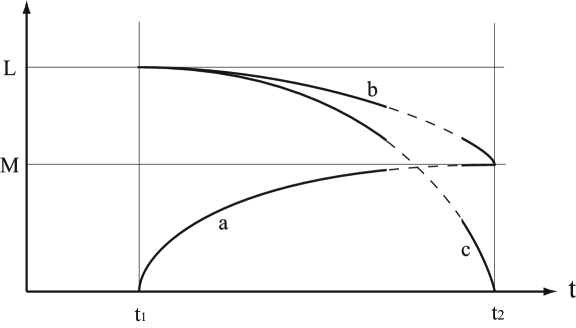
Figure 2: An illustration of the Tod-Hitchin metric

In particular, for the exact solutions (2.10)-(2.14), the parameters $(\delta,M,\Lambda)$ are given by

(a)

$k=3$ :  $(1,\,\sqrt{3},\,3),~{}~{}0\leq t\leq\pi/3.$

(b)

$k=4$ :  $(3/4,\,1/\sqrt{2},\,6),~{}~{}0\leq t\leq\pi/4.$

(c)

$k=6$ :  $(5\sqrt{6}/72,\,1/\sqrt{3},\,3),~{}~{}0\leq r\leq\infty.$

(d)

$k=8$ :  $(63\sqrt{3}/2048,\,\sqrt{3-2\sqrt{2}},\,3),~{}~{}\sqrt{2}-1\leq r\leq 1.$

When we consider the case with large $k$, the expansion (2.18) implies that the biaxial solutions approximate well the Tod-Hitchin metrics near the boundary $t=t_{1}$. We find that the ASD Taub-NUT de-Sitter solution $g_{k}$ exactly reproduces the expansion (2.18) with $\delta=0$. In the limit $k\rightarrow\infty$, the equation (2.18) yields $b(t)\sim c(t)$, which is consistent with the asymptotic behavior of the Atiyah-Hitchin metric. Indeed, the Atiyah-Hitchin metric behaves like the ASD Taub-NUT metric with exponentially-small corrections [18].

The Atiyah-Hitchin manifold is identified as the moduli space of the three-dimensional ${\mathcal{N}}=4$ SU(2) gauge theory[19][20]. The vacuum expectation values of bosonic fields of the theory, three SO(3) scalars $\phi_{i}$ and one scalar $\sigma$ dual of photon, parameterize the Atiyah-Hitchin manifold. The hyperkähler structure of the Atiyah-Hitchin manifold ensures the ${\mathcal{N}}=4$ supersymmetry. In the region of large $\left<\phi_{i}\right>$, the monopole correction is suppressed and the moduli is well approximated by the Taub-NUT geometry with a negative charge. On the other hand, near the origin, the Tod-Hitchin geometry provides a good approximation even if $k$ is small, and thus one can expect that the gauge theory near the origin of the moduli is well described by that with the Tod-Hitchin geometry as the moduli. In this approximation, the metric on the moduli becomes simpler but the gauge theory fails to be supersymmetric. This is because the Tod-Hitchin geometry is not Kähler, while the Atiyah-Hitchin manifold is hyperkähler. As we have seen, the Tod-Hitchin geometry converges to the Atiyah-Hitchin manifold in the limit, $k\to\infty$ together with $\Lambda\to 0$. It is interesting to consider the gauge theory with the Tod-Hitchin geometry as the moduli and to reveal the role of the limit. In this limit, the supersymmetry recovers and the moduli becomes non compact by sending the orbifold singularity of the Tod-Hitchin geometry to infinity. On the other hand, to study the region near the orbifold singularity, it will be useful to examine the theory with the Taub-NUT de Sitter geometry as the moduli. These are left for future investigations.

3 Einstein metrics on compact weak $G_{2}$ manifolds

In this section we shall describe seven-dimensional geometries based on ASD Bianchi IX orbifolds ${\mathcal{O}_{k}}$ with the Tod-Hitchin metrics $g^{\rm TH}_{k}$. As discussed in the previous section, the Tod-Hitchin metric is defined on $S^{4}$ with an orbifold singularity parameterized by the integer $k$. However, we shall show that a principal SO(3) bundle $M_{k}\rightarrow{\mathcal{O}_{k}}$ is actually smooth and the total space $M_{k}$ admits Einstein metrics of weak holonomy $G_{2}$. In this way, we obtain an infinite series of seven-dimensional compact Einstein manifolds.

Let $\phi$ be an SO(3)-connection on $M_{k}$; it is locally written as

$$\phi=s^{-1}As+s^{-1}ds~{},\quad s\in SO(3).$$ (3.1)

Here, $A$ is an so(3)-valued local one-form on ${\mathcal{O}_{k}}$ and $s^{-1}ds$ is regarded as the Maurer-Cartan form. We let $\phi^{i}$ denote the component of the connection with respect to the standard basis $\{E^{i}\}$ of so(3) which satisfies the Lie bracket relation $[E^{i},E^{j}]=\epsilon_{ijk}E^{k}$. The left-invariant one-forms $\tilde{\sigma_{i}}$ are defined by $s^{-1}ds=\tilde{\sigma_{i}}E^{i}$ and so the equation (3.1) may be written as $\phi^{i}=s_{ji}A^{j}+\tilde{\sigma_{i}}$ by using the adjoint representation $s^{-1}E^{i}s=s_{ij}E^{j}$. Given a metric $\alpha=(\alpha_{ij})$ on SO(3), then the Kaluza-Klein metric on $M_{k}$ takes the form,

$${\boldsymbol{g}}_{k}=\alpha_{ij}\phi^{i}\phi^{j}+g^{\rm TH}_{k}~{}.$$ (3.2)

The Einstein equation can be solved by imposing the following conditions:

(1)

$A^{i}$ is an SO(3) Yang-Mills instanton on ${\mathcal{O}_{k}}$.

(2)

The metric $\alpha$ has a diagonal form; $\alpha=\mbox{diag}(\alpha_{1}^{2},\alpha_{2}^{2},\alpha_{3}^{2})$ where $\alpha_{i}$ are constants.

The instanton is given by the self-dual spin connection, $A^{i}=-\omega_{0i}-\frac{1}{2}\epsilon_{ijk}\omega_{jk}$ . Using the explicit formula (A.4), it is written as $A^{i}=K_{i}\sigma_{i}$ with

$$K_{1} = \dot{a}+\frac{-a^{2}+b^{2}+c^{2}}{2bc}~{},$$

$$K_{2} = \dot{b}+\frac{a^{2}-b^{2}+c^{2}}{2ac}~{},$$ (3.3)

$$K_{3} = \dot{c}+\frac{a^{2}+b^{2}-c^{2}}{2ab}~{}.$$

Thus, the seven-dimensional Einstein equations with cosmological constant $\lambda$ are equivalent to

$$\frac{\alpha_{1}^{4}-(\alpha_{2}^{2}-\alpha_{3}^{2})^{2}}{2\alpha_{1}^{2}\alpha_{2}^{2}\alpha_{3}^{2}}+\left(\frac{\Lambda}{3}\right)^{2}\alpha_{1}^{2}=\lambda,\quad\Lambda-\frac{1}{2}\left(\frac{\Lambda}{3}\right)^{2}(\alpha_{1}^{2}+\alpha_{2}^{2}+\alpha_{3}^{2})=\lambda,$$ (3.4)

and the two equations with cyclic permutation of $\alpha_{1},\alpha_{2},\alpha_{3}$. These can be solved easily, and one has two solutions,

$$\alpha=\beta_{\ell}\,\mbox{diag}(1,1,1),\quad\beta_{\ell}=\frac{3}{\ell\Lambda}$$ (3.5)

with $\lambda=\Lambda\frac{2\ell-1}{2\ell}$ ($\ell$=1 or $5$). Using the right-invariant one-forms $\hat{\sigma_{i}}$ ($sds^{-1}=\hat{\sigma_{i}}E^{i}$) and the Tod-Hitchin metric in the form (2.1), we find two types of seven-dimensional Einstein metrics;

$${\boldsymbol{g}}_{k}^{(\ell)}=dt^{2}+a^{2}(t)\sigma_{1}^{2}+b^{2}(t)\sigma_{2}^{2}+c^{2}(t)\sigma_{3}^{2}+\beta_{\ell}(K_{i}(t)\sigma_{i}-\hat{\sigma_{i}})^{2}~{}.$$ (3.6)

The conditions (1) and (2) also induce a $G_{2}$-structure on $M_{k}$ as follows: Recall that the $G_{2}$-structure is characterized by a global one-form $\omega$, which is written locally as

$$\omega = \theta^{1}\wedge\theta^{2}\wedge\theta^{3}+\theta^{1}\wedge(\theta^{4}\wedge\theta^{5}+\theta^{6}\wedge\theta^{7})~{}$$ (3.7)

$$+ \theta^{2}\wedge(\theta^{4}\wedge\theta^{6}+\theta^{7}\wedge\theta^{5})+\theta^{3}\wedge(\theta^{4}\wedge\theta^{7}+\theta^{5}\wedge\theta^{6})~{},$$

where {$\theta^{\alpha};\alpha=1,2,\dots 7$ } is a fixed orthonormal basis of the seven-dimensional metric ${\boldsymbol{g}}_{diag}$ (see appendix C). The condition of weak holonomy $G_{2}$ is defined by $d\omega=c*\omega$ where $*$ is the Hodge star operation associated to ${\boldsymbol{g}}_{diag}$ and $c$ is a constant. Under (1) and (2), the weak $G_{2}$ condition reproduces the metric (3.6). The holonomy group $\mbox{Hol}(\bar{\boldsymbol{g}}_{k}^{(\ell)})$ of the metric cone $(C(M_{k}),\bar{\boldsymbol{g}}_{k}^{(\ell)})=(R_{+}\times M_{k},d\tau^{2}+\tau^{2}{\boldsymbol{g}}_{k}^{(\ell)})$ is contained in Spin(7) [22][23]:

(A)

$\mbox{Hol}(\bar{\boldsymbol{g}}_{k}^{(1)})=$ Sp(2) $\subset$ Spin(7) and $(M_{k},{\boldsymbol{g}}_{k}^{(1)})$ is a 3-Sasakian manifold.

(B)

$\mbox{Hol}(\bar{\boldsymbol{g}}_{k}^{(5)}))$ = Spin(7) and $(M_{k},{\boldsymbol{g}}_{k}^{(5)}))$ is a proper $G_{2}$ manifold.

We now proceed to a discussion of the metric singularities. The orbifold singularity of the base space ${\mathcal{O}_{k}}$ emerges at the boundaries where a certain component of the metric vanishes. To understand the effect of this singularity in the total space $M_{k}$, it is useful to see the behavior of the metric ${\boldsymbol{g}}_{k}^{(\ell)}$ with weak holonomy $G_{2}$ near boundaries. From (2.18) and ((2)), putting $\Omega(k)=k^{2}+(k-2)^{2}$ we find

$${\boldsymbol{g}}_{k}^{(\ell)} \rightarrow dt^{2}+\frac{4t^{2}}{\Omega^{2}(k)}((k-2)\sigma_{1}+k\hat{\sigma_{1}})^{2}$$ (3.8)

$$+\frac{\ell\beta_{\ell}k}{k-2}(\sigma_{2}^{2}+\sigma_{3}^{2})+\beta_{\ell}(\hat{\sigma_{2}}^{2}+\hat{\sigma_{3}}^{2})+\frac{\beta_{\ell}}{(k-2)^{2}}(k\sigma_{1}-(k-2)\hat{\sigma_{1}})^{2}$$

for $t\rightarrow t_{1}$, and

$${\boldsymbol{g}}_{k}^{(\ell)} \rightarrow dt^{2}+\frac{t^{2}}{25}(\sigma_{3}+3\hat{\sigma_{3}})^{2}$$ (3.9)

$$+M^{2}(\sigma_{1}^{2}+\sigma_{2}^{2})+\beta_{\ell}(\hat{\sigma_{1}}^{2}+\hat{\sigma_{2}}^{2})+\beta_{\ell}(3\sigma_{3}-\hat{\sigma_{3}})^{2}$$

for $t\rightarrow t_{2}$. These expressions correspond to the asymptotic forms (2.15) and (2.16) of the Tod-Hitchin metric. An important difference is that the collapsing circle is twisted by the fiber SO(3), which allows us to resolve the orbifold singularity of ${\mathcal{O}_{k}}$ as shown below. Let us represent the invariant one-forms $\sigma_{i},\hat{\sigma_{j}}$ in terms of Euler’s angles:

$$\sigma_{1} = d\psi+\cos\theta d\phi,\quad\hat{\sigma}_{1}=-d\hat{\phi}-\cos\hat{\theta}d\hat{\psi},$$

$$\sigma_{2} = \cos\psi d\theta+\sin\psi\sin\theta d\phi,\quad\hat{\sigma}_{2}=-\cos\hat{\phi}d\hat{\theta}-\sin\hat{\phi}\sin\hat{\theta}d\hat{\psi},$$

$$\sigma_{3} = -\sin\psi d\theta+\cos\psi\sin\theta d\phi,\quad\hat{\sigma}_{3}=-\sin\hat{\phi}d\hat{\theta}+\cos\hat{\phi}\sin\hat{\theta}d\hat{\psi}~{}.$$ (3.10)

The following transformation

$$\eta=\frac{2}{\Omega(k)}((k-2)\psi-k\hat{\phi}),\quad\chi=k\psi+(k-2)\hat{\phi}~{},$$ (3.11)

yields

$${\boldsymbol{g}}_{k}^{(\ell)} \rightarrow dt^{2}+t^{2}\left(d\eta+\frac{2(k-2)}{\Omega(k)}\cos\theta d\phi-\frac{2k}{\Omega(k)}\cos\hat{\theta}d\hat{\psi}\right)^{2}$$ (3.12)

$$+\frac{\ell\beta_{\ell}k}{k-2}(d\theta^{2}+\sin^{2}\theta d\phi^{2})+\beta_{\ell}(d\hat{\theta}^{2}+\sin^{2}\hat{\theta}d\hat{\psi}^{2})$$

$$+\frac{\beta_{\ell}}{(k-2)^{2}}(d\chi+k\cos\theta d\phi+(k-2)\cos\hat{\theta}d\hat{\psi})^{2}$$

for $t\rightarrow t_{1}$. From (3.11) we have $d\eta\wedge d\chi=2(d\psi\wedge\hat{\phi})$. It follows that one can adjust the ranges of the new angles as $0\leq\eta<2\pi$, $0\leq\chi<4\pi$ since Euler’s angles have the ranges $0\leq\psi<2\pi$, $0\leq\hat{\phi}<2\pi$. Thus, the metric ${\boldsymbol{g}}_{k}^{(\ell)}$ extends smoothly over the circle bundle $T^{k,k-2}$ with the squashed metric

$$g_{bolt}=\frac{\ell k}{k-2}(d\theta^{2}+\sin^{2}\theta d\phi^{2})+d\hat{\theta}^{2}+\sin^{2}\hat{\theta}d\hat{\psi}^{2}$$

$$+\frac{1}{(k-2)^{2}}(d\chi+k\cos\theta d\phi+(k-2)\cos\hat{\theta}d\hat{\psi})^{2}$$ (3.13)

at the boundary $t=t_{1}$. Also, similar arguments show that the metric extends over $T^{3,1}$ at $t=t_{2}$.

4 Geodesics on weak $G_{2}$ manifolds

In this section, we consider a Hamiltonian formulation describing geodesics on the weak $G_{2}$ manifold $M_{k}$. The phase space is the cotangent bundle $T^{*}M_{k}$ with coordinates $(x^{\alpha})=(t,\theta,\phi,\psi,\hat{\theta},\hat{\phi},\hat{\psi})$ and their conjugate momenta $(p_{\alpha})$. The equations for geodesic flow are the canonical equations on $T^{*}M_{k}$ with Hamiltonian $H=\frac{1}{2}g^{\alpha\beta}p_{\alpha}p_{\beta}$. Using the metric (3.6), we may write explicitly as

$$H = \frac{1}{2}p_{t}^{2}+\frac{1}{2}\left(\frac{L_{1}^{2}}{a^{2}}+\frac{L_{2}^{2}}{b^{2}}+\frac{L_{3}^{2}}{c^{2}}\right)+\frac{1}{2\beta_{\ell}}(\hat{R}_{1}^{2}+\hat{R}_{2}^{2}+\hat{R}_{3}^{2})$$ (4.1)

$$+ \frac{1}{2}\left(\frac{K_{1}^{2}\hat{R}_{1}^{2}}{a^{2}}+\frac{K_{2}^{2}\hat{R}_{2}^{2}}{b^{2}}+\frac{K_{3}^{2}\hat{R}_{3}^{2}}{c^{2}}\right)+\frac{K_{1}L_{1}\hat{R}_{1}}{a^{2}}+\frac{K_{2}L_{2}\hat{R}_{2}}{b^{2}}+\frac{K_{3}L_{3}\hat{R}_{3}}{c^{2}}.$$

The functions $L_{i}$ and $\hat{R}_{j}$ are canonically conjugate to $\sigma_{i}$ and $\hat{\sigma_{j}}$, respectively:

$$L_{1} = p_{\psi}~{},$$

$$L_{2} = -\cot\theta\sin\psi p_{\psi}+\cos\psi p_{\theta}+\frac{\sin\psi}{\sin\theta}p_{\phi}~{},$$

$$L_{3} = -\cot\theta\cos\psi p_{\psi}-\sin\psi p_{\theta}+\frac{\cos\psi}{\sin\theta}p_{\phi}~{},$$

$$\hat{R}_{1} = -p_{\hat{\phi}}~{},$$

$$\hat{R}_{2} = \cot\hat{\theta}\sin\hat{\phi}p_{\hat{\phi}}-\cos\hat{\phi}p_{\hat{\theta}}-\frac{\sin\hat{\phi}}{\sin\theta}p_{\hat{\psi}}~{},$$

$$\hat{R}_{3} = -\cot\hat{\theta}\cos\hat{\phi}p_{\hat{\phi}}-\sin\hat{\phi}p_{\hat{\theta}}+\frac{\cos\hat{\phi}}{\sin\hat{\theta}}p_{\hat{\psi}}~{},$$ (4.2)

which satisfy the SO(3) $\times$ SO(3) relations, $\{L_{i},L_{j}\}=-\epsilon_{ijk}L_{k}$ and $\{\hat{R}_{i},\hat{R}_{j}\}=-\epsilon_{ijk}\hat{R}_{k}$. We also introduce functions $\hat{L}_{i}$ and $R_{j}$ by exchanging Euler’s angles, $(\theta,\phi,\psi)\leftrightarrow(\hat{\theta},\hat{\phi},\hat{\psi})$. Then, one can easily show that they express the isometry SO(3) $\times$ SO(3) of the metric; $\{L_{i},R_{j}\}=\{\hat{L}_{i},\hat{R}_{j}\}=0$ and hence $\{H,\hat{L}_{i}\}=\{H,R_{j}\}=0$. It should be noticed that in general neither $L_{i}$ nor $\hat{R}_{j}$ are conserved, although $\sum_{i}L_{i}^{2}=\sum_{i}R_{i}^{2}$ and $\sum_{i}\hat{L}_{i}^{2}=\sum_{i}\hat{R}_{i}^{2}$ are conserved quantities, the second Casimir. The relation between $L_{i}~{}(\hat{L_{i}})$ and $R_{i}~{}(\hat{R}_{i})$ corresponds to the relation between left and right actions of SO(3). The Hamiltonian equations $\frac{df}{d\tau}=\{f,H\}$ are

$$\frac{dL_{1}}{d\tau} = \left(\frac{1}{c^{2}}-\frac{1}{b^{2}}\right)L_{2}L_{3}-\frac{K_{2}}{b^{2}}L_{3}\hat{R}_{2}+\frac{K_{3}}{c^{2}}L_{2}\hat{R}_{3}~{},$$

$$\frac{dL_{2}}{d\tau} = \left(\frac{1}{a^{2}}-\frac{1}{c^{2}}\right)L_{3}L_{1}-\frac{K_{3}}{c^{2}}L_{1}\hat{R}_{3}+\frac{K_{1}}{a^{2}}L_{3}\hat{R}_{1}~{},$$

$$\frac{dL_{3}}{d\tau} = \left(\frac{1}{b^{2}}-\frac{1}{a^{2}}\right)L_{1}L_{2}-\frac{K_{1}}{a^{2}}L_{2}\hat{R}_{1}+\frac{K_{2}}{b^{2}}L_{1}\hat{R}_{2}~{},$$ (4.3)

and

$$\frac{d\hat{R}_{1}}{d\tau} = \left(\left(\frac{K_{3}}{c}\right)^{2}-\left(\frac{K_{2}}{b}\right)^{2}\right)\hat{R}_{2}\hat{R}_{3}-\frac{K_{2}}{b^{2}}\hat{R}_{3}L_{2}+\frac{K_{3}}{c^{2}}\hat{R}_{2}L_{3}~{},$$

$$\frac{d\hat{R}_{2}}{d\tau} = \left(\left(\frac{K_{1}}{a}\right)^{2}-\left(\frac{K_{3}}{c}\right)^{2}\right)\hat{R}_{3}\hat{R}_{1}-\frac{K_{3}}{c^{2}}\hat{R}_{1}L_{3}+\frac{K_{1}}{a^{2}}\hat{R}_{3}L_{1}~{},$$

$$\frac{d\hat{R}_{3}}{d\tau} = \left(\left(\frac{K_{2}}{b}\right)^{2}-\left(\frac{K_{1}}{a}\right)^{2}\right)\hat{R}_{1}\hat{R}_{2}-\frac{K_{1}}{a^{2}}\hat{R}_{2}L_{1}+\frac{K_{2}}{b^{2}}\hat{R}_{1}L_{2}~{}$$ (4.4)

together with

$$\frac{dt}{d\tau} = p_{t}~{},$$

$$\frac{dp_{t}}{d\tau} = \frac{\dot{a}}{a^{3}}L_{1}^{2}+\frac{\dot{b}}{b^{3}}L_{2}^{2}+\frac{\dot{c}}{c^{3}}L_{3}^{2}$$ (4.5)

$$-\frac{K_{1}}{a}\left(\frac{\dot{K_{1}}}{a}-\frac{K_{1}\dot{a}}{a^{2}}\right)\hat{R}_{1}^{2}-\frac{K_{2}}{b}\left(\frac{\dot{K_{2}}}{b}-\frac{K_{2}\dot{b}}{b^{2}}\right)\hat{R}_{2}^{2}-\frac{K_{3}}{c}\left(\frac{\dot{K_{3}}}{c}-\frac{K_{3}\dot{c}}{c^{2}}\right)\hat{R}_{3}^{2}$$

$$-\left(\frac{\dot{K_{1}}}{a^{2}}-2\frac{K_{1}\dot{a}}{a^{3}}\right)L_{1}\hat{R}_{1}-\left(\frac{\dot{K_{2}}}{b^{2}}-2\frac{K_{2}\dot{b}}{b^{3}}\right)L_{2}\hat{R}_{2}-\left(\frac{\dot{K_{3}}}{c^{2}}-2\frac{K_{3}\dot{c}}{c^{3}}\right)L_{3}\hat{R}_{3}~{}.$$

This system may be regarded as an interacting rigid body system with angular momenta $L_{i}$ and $\hat{R}_{j}$. The moments of inertia are given by $(I_{i})=(a,b,c)$ and $(\hat{I}_{i})=(a/K_{1},b/K_{2},c/K_{3})$, which have a non-trivial time dependence through the equation (4.5). When we put $K_{i}=0$, then the interaction between $L_{i}$ and $\hat{R}_{j}$ vanishes. Thus, the angular momenta $\hat{R}_{j}$ are constants, and the remaining equations (4.3) and (4.5) describe the geodesics on the Tod-Hitchin manifold [11][18][24].

As a special solution, consider the case $L_{2}=\hat{R}_{2}=0$ in the equations (4.3)-(4.5). Then, the angular momenta $(L_{1},L_{3})$ and $(\hat{R}_{1},\hat{R}_{3})$ are constants. If we can find a parameter $t_{0}$ such that $a(t_{0})=c(t_{0})$, we have $\frac{dL_{2}}{d\tau}=\frac{d\hat{R}_{2}}{d\tau}=0$ after setting

$$K_{3} (t_{0})L_{1}\hat{R}_{3}-K_{1}(t_{0})L_{3}\hat{R}_{1}=0~{},$$

$$( K_{1}^{2} (t_{0})-K_{3}^{2}(t_{0}))\hat{R}_{3}\hat{R}_{1}-K_{3}(t_{0})L_{3}\hat{R}_{1}+K_{1}(t_{0})L_{1}\hat{R}_{3}=0~{}.$$ (4.6)

In fact, one can show that the parameter $t_{0}$ exists from the behavior of the Painlevé VI solution (see Figure 2). Finally, the equation $p_{t}=0$ requires the further constraint for the angular momenta:

$$\frac{\dot{a}}{a} L_{1}^{2} +\frac{\dot{c}}{c}L_{3}^{2}+K_{1}\left(\frac{a\Lambda}{3}+K_{1}\frac{\dot{a}}{a}\right)\hat{R}_{1}^{2}+K_{3}\left(\frac{a\Lambda}{3}+K_{3}\frac{\dot{c}}{c}\right)\hat{R}_{3}^{2}$$ (4.7)

$$+ \left(\frac{a\Lambda}{3}+2K_{1}\frac{\dot{a}}{a}\right)L_{1}\hat{R}_{1}+\left(\frac{a\Lambda}{3}+2K_{3}\frac{\dot{c}}{c}\right)L_{3}\hat{R}_{3}=0~{},$$

where we have used an identity $\dot{K}_{1}=\dot{K}_{3}=-a\Lambda/3$ at $a=c$. If we consider the case $\hat{R}_{1}=\hat{R}_{3}=0$, the equation (4.6) is automatically satisfied, and (4.7) yields $(L_{1}/L_{3})^{2}=-(\dot{c}/\dot{a})(t_{0})$[24]. As a result, we find a class of geodesics on $M_{k}$. For cases $k=3,4,6$ and 8 given by (2.10)-(2.14), the solutions are summarized as follows:

(a)

$k=3$ :  $t_{0}=\pi/6$
$\frac{L_{1}}{L_{3}}=\pm 1,~{}~{}\hat{R}_{1}=\hat{R}_{3}=0,$
$\frac{L_{1}}{\hat{R}_{3}}=\frac{\hat{R}_{1}}{\hat{R}_{3}}-\sqrt{3},~{}~{}\frac{L_{3}}{\hat{R}_{3}}=1+\sqrt{3},$
$\frac{L_{1}}{\hat{R}_{1}}=-2/(1+\sqrt{3})$  and $-13/(3+4\sqrt{3}),~{}~{}L_{3}=\hat{R}_{3}=0.$

(b)

$k=4$ :  $t_{0}=\pi/6$
$\frac{L_{1}}{L_{3}}=\pm 2,~{}~{}\hat{R}_{1}=\hat{R}_{3}=0,$
$\frac{L_{1}}{\hat{R}_{3}}=-\sqrt{3}~{}\frac{\hat{R}_{1}}{\hat{R}_{3}},~{}~{}\frac{L_{3}}{\hat{R}_{3}}=\sqrt{3}/2,$
$\frac{L_{1}}{\hat{R}_{1}}=\sqrt{3}$  and $-4\sqrt{3}/3,~{}~{}L_{3}=\hat{R}_{3}=0.$

(c)

$k=6$ :  $r_{0}=2^{1/3}+2^{-1/3}\cong 2.05$
$\frac{L_{1}}{L_{3}}\cong\pm 1.92,~{}~{}\hat{R}_{1}=\hat{R}_{3}=0,$
$\frac{L_{1}}{\hat{R}_{1}}\cong-1.71$ and $-1.28$,   $L_{3}=\hat{R}_{3}=0,$
$\frac{L_{3}}{\hat{R}_{3}}\cong 0.95$ and 1.06,   $L_{1}=\hat{R}_{1}=0.$

(d)

$k=8$ :  $r_{0}\cong 0.55$
$\frac{L_{1}}{L_{3}}\cong\pm 2.21,~{}~{}\hat{R}_{1}=\hat{R}_{3}=0,$
$\frac{L_{1}}{\hat{R}_{1}}\cong-1.15,~{}~{}\frac{L_{3}}{\hat{R}_{1}}\cong\pm 0.50,~{}~{}\frac{\hat{R}_{3}}{\hat{R}_{1}}\cong\pm 0.52,$
$\frac{L_{1}}{\hat{R}_{1}}\cong-1.46$ and $-1.15$,   $L_{3}=\hat{R}_{3}=0,$
$\frac{L_{3}}{\hat{R}_{3}}\cong 0.97$ and 1.03,   $L_{1}=\hat{R}_{1}=0.$

5 M-theory on AdS${}_{4}\times M_{k}$

We have constructed infinitely many compact Einstein manifolds $M_{k}$, which are 3-Sasakian manifolds for $\ell=1$ and proper weak $G_{2}$ manifolds for $\ell=5$. The orbifold singularity of the Tod-Hitchin geometry has been resolved by having additional dimensions, so that we can expect the resolution of the orbifold singularity in the moduli by adding scalars in the corresponding gauge theory. The resulting seven-dimensional manifolds $M_{k}$ admit 3-Sasakian or proper weak $G_{2}$ structures, and thus the gauge theories are ${\mathcal{N}}=3$ supersymmetric for $\ell=1$, while ${\mathcal{N}}=1$ supersymmetric for $\ell=5$. It was shown that the manifold $M_{3}(\ell=1)=N^{0,1,0}$ appears as the moduli space of an ${\mathcal{N}}=3$ gauge theory [25]. We expect that the seven-dimensional manifolds $M_{k}$ with general $k$ also emerge as the moduli spaces of three-dimensional ${\mathcal{N}}=3$ or ${\mathcal{N}}=1$ supersymmetric gauge theories. It is interesting to achieve this and to reveal the role of $k$ from the viewpoint of gauge theories. Leaving this interesting issue as a future problem, in this section we consider M-theory on AdS${}_{4}\times M_{k}$, and apply the AdS/CFT correspondence.

Using the 3-Sasakian or proper weak $G_{2}$ manifolds $M_{k}$, one can construct supersymmetric M-theory solutions, AdS${}_{4}\times M_{k}$, which are AdS/CFT dual to three-dimensional superconformal field theories. The isometry of $M_{k}$ corresponds to the global symmetry of the dual superconformal field theories, including the R-symmetry. The manifolds $M_{k}$ contain S⁷, $N^{0,1,0}$ and squashed S⁷ ($\tilde{S}^{7}$) as special homogeneous cases; $M_{3}(\ell=1)$, $M_{4}(\ell=1)$ and $M_{3}(\ell=5)$, respectively. For these cases, the dual three-dimensional gauge theories which flow to the superconformal field theories at the IR are the ${\mathcal{N}}=8$ gauge theory without flavor [2] for S⁷ with SO(8) isometry, the ${\mathcal{N}}=3$ gauge theory with SU(3) flavor [25][N^0, 1] for $N^{0,1,0}$ with SU(3)$\times$SU(2) isometry. The squashed S⁷ admits SO(5)$\times$SO(3) isometry so that the dual theory is expected to be ${\mathcal{N}}=1$ gauge theory with SO(5)$\times$SO(3) flavor. For generic $k$, because the metrics on $M_{k}$ admit SO(3)$\times$SO(3) isometry as shown in section 4, the gauge theories which flow to the superconformal field theories at the IR are an ${\mathcal{N}}=3$ gauge theory with SO(3) flavors for $\ell=1$, and an ${\mathcal{N}}=1$ gauge theory with SO(3)$\times$SO(3) flavors for $\ell=5$. Since it is not easy to extract the Kaluza-Klein spectrum on $M_{k}$ as is expected from the analysis in section 4, we assume this correspondence here. The UV limit of the theory is described by ${\mathbb{R}}^{1,2}\times C(M_{k})$, where $C(M_{k})$ stands for the cone over $M_{k}$. The cone metric are hyperkähler for $\ell=1$ and Spin(7) for $\ell=5$. For the homogeneous cases S⁷, $N^{0,1,0}$ and $\tilde{S}^{7}$, the holographic RG-flows which interpolate ${\mathbb{R}}^{1,2}\times C(M_{k})$ at UV and AdS${}_{4}\times M_{k}$ at IR are examined in [27]. For general $k$, the brane solution which describes the holographic RG-flow from ${\mathbb{R}}^{1,2}\times C(M_{k})$ at UV to AdS${}_{4}\times M_{k}$ at IR is

$$g_{11}=H^{-\frac{2}{3}}g_{{\mathbb{R}}^{1,2}}+H^{\frac{1}{3}}\bar{\boldsymbol{g}}_{k}^{(\ell)}~{},~{}~{}~{}~{}F={\rm dvol}({\mathbb{R}}^{1,2})\wedge dH^{-1}~{},~{}~{}~{}~{}H=1+\left(\frac{a}{r}\right)^{6},$$ (5.1)

where $a=(2^{5}\pi^{2}N)^{\frac{1}{6}}\ell_{P}$ and $\bar{\boldsymbol{g}}_{k}^{(\ell)}=dr^{2}+r^{2}{\boldsymbol{g}}_{k}^{(\ell)}$. This corresponds to $N$ coincident M2-branes at $r=0$. For small $r$, the brane solution (5.1) reduces to the product metric of $M_{k}$ with cosmological constant $1/a^{2}$ and AdS₄ with $4/a^{2}$, and the four-form strength $F=6$ dvol(AdS₄)$/a$. On the other hand, for large $r$, (5.1) approaches the product metric of ${\mathbb{R}}^{1,2}$ and $C(M_{k})$ without the four-form strength. It is interesting to examine the limit, $k\to\infty$ together with $\Lambda\to 0$, in which the four-dimensional base space, Tod-Hitchin geometry, converges to the Atiyah-Hitchin hyperkähler manifold $M_{AH}$. The limit $\Lambda\to 0$ corresponds to the limit $a\to\infty$, because the cosmological constant $\lambda=\Lambda\frac{2\ell-1}{2\ell}$ of $M_{k}$ is now ${1}/{a^{2}}$. In this limit, (5.1) approaches the metric on ${\mathbb{R}}^{1,3}\times{\mathbb{R}}^{3}/{\mathbb{Z}}_{2}\times M_{AH}$ without the four-form strength because $M_{k}$ reduces to ${\mathbb{R}}^{3}/{\mathbb{Z}}_{2}\times M_{AH}$. Apart from the ${\mathbb{Z}}_{2}$ factor, this solution can be regarded as an orientifold 6-plane of the IIA superstring theory, and thus the $g_{11}$ provides an approximation of the orientifold plane.

Infinitely many inhomogeneous Einstein metrics on compact manifolds are derived from Kerr de-Sitter black holes as the Page limit in [28][29][30], and those with a Sasaki structure found in [31] as the Sasaki-Einstein twist in [32]. It is interesting to consider the black hole solutions corresponding to $M_{k}$ constructed in this paper. We have discussed the holographic RG-flow from ${\mathbb{R}}^{1,2}\times C(M_{k})$ to AdS${}_{4}\times M_{k}$. In [33], a transition from AdS${}_{4}\times\tilde{S}^{7}$ to AdS${}_{4}\times S^{7}$ is discussed. It is expected that there is a similar transition from AdS${}_{4}\times M_{k}(\ell=5)$ to AdS${}_{4}\times M_{k}(\ell=1)$. We leave these issues for future investigations.

Note added: After submitting this paper to e-print archives, we received from K. Galicki the draft [34] of a talk given by W. Ziller, which is refereed in [8]. In the draft, Grove, Wilking and Ziller proved that 3-Sasakian orbifolds $M_{k}(\ell=1)$ corresponding to AdS Bianchi IX orbifolds ${\mathcal{O}}_{k}$ with the Tod-Hitchin metrics are manifolds with the following properties: (a) for odd $k$, they have the same cohomology ring as an S³-bundle over S⁴, (b) for even $k$, they have the same cohomology ring as a general Aloff Wallach space, (c) in both cases, it carries an invariant cohomogeneity one structure by S${}^{3}\times$S³. In addition, we were informed by K. Galicki that the proper weak $G_{2}$ orbifolds $M_{k}(\ell=5)$ can be also made smooth by the method of K. Galicki and S. Salamon [23].

Our study provides a concrete procedure to resolve orbifold singularities which is familiar to physicists, and the explicit forms of the 3-Sasakian and proper weak $G_{2}$ metrics.

Appendix A four-dimensional ASD Einstein manifolds

The Bianchi IX metric is of the form

$$g=dt^{2}+a^{2}(t)\sigma_{1}^{2}+b^{2}(t)\sigma_{2}^{2}+c^{2}(t)\sigma_{3}^{2}~{},$$ (A.1)

where $\sigma_{i}$ are left-invariant one-forms on SO(3) ,

$$d\sigma_{i}=-\frac{1}{2}\epsilon_{ijk}\sigma_{j}\wedge\sigma_{k}.$$ (A.2)

Defining vielbein

$$e^{0}=dt,~{}~{}~{}e^{1}=a\sigma_{1},~{}~{}~{}e^{2}=b\sigma_{2},~{}~{}~{}e^{3}=c\sigma_{3},$$ (A.3)

one evaluates the spin connection as

$$\omega_{01} = -\frac{\dot{a}}{a}~{}e^{1}~{},~{}~{}~{}~{}\omega_{12}=-\frac{a^{2}+b^{2}-c^{2}}{2abc}~{}e^{3}~{},$$

$$\omega_{02} = -\frac{\dot{b}}{b}~{}e^{2}~{},~{}~{}~{}~{}\omega_{31}=-\frac{a^{2}-b^{2}+c^{2}}{2abc}~{}e^{2}~{},$$

$$\omega_{03} = -\frac{\dot{c}}{c}~{}e^{3}~{},~{}~{}~{}~{}\omega_{23}=-\frac{-a^{2}+b^{2}+c^{2}}{2abc}~{}e^{1}~{}.$$ (A.4)

The Einstein equations $R_{\alpha\beta}=\Lambda\delta_{\alpha\beta}$ are given by

$$\frac{\ddot{a}}{a} + \frac{\ddot{b}}{b}+\frac{\ddot{c}}{c}+\Lambda=0~{},$$

$$\frac{\ddot{a}}{a} + \frac{\dot{a}}{a}\left(\frac{\dot{b}}{b}+\frac{\dot{c}}{c}\right)-\frac{a^{4}-(b^{2}-c^{2})^{2}}{2a^{2}b^{2}c^{2}}+\Lambda=0~{},$$

$$\frac{\ddot{b}}{b} + \frac{\dot{b}}{b}\left(\frac{\dot{a}}{a}+\frac{\dot{c}}{c}\right)-\frac{b^{4}-(a^{2}-c^{2})^{2}}{2a^{2}b^{2}c^{2}}+\Lambda=0~{},$$

$$\frac{\ddot{c}}{c} + \frac{\dot{c}}{c}\left(\frac{\dot{a}}{a}+\frac{\dot{b}}{b}\right)-\frac{c^{4}-(a^{2}-b^{2})^{2}}{2a^{2}b^{2}c^{2}}+\Lambda=0~{}.$$ (A.5)

The ASD condition further requires the following equations:

$$\frac{\ddot{a}}{a}~{} + \left(C\frac{\dot{b}}{b}+B\frac{\dot{c}}{c}-\frac{\dot{a}}{bc}\right)+\frac{\Lambda}{3}=0~{},$$

$$\frac{\ddot{b}}{b}~{} + \left(C\frac{\dot{a}}{a}+A\frac{\dot{c}}{c}-\frac{\dot{b}}{ac}\right)+\frac{\Lambda}{3}=0~{},$$

$$\frac{\ddot{c}}{c} + \left(B\frac{\dot{a}}{a}+A\frac{\dot{b}}{b}-\frac{\dot{c}}{ab}\right)+\frac{\Lambda}{3}=0~{},$$

$$\frac{\dot{a}\dot{b}}{ab}~{} - \frac{a^{4}+b^{4}-3c^{4}+2(-a^{2}b^{2}+b^{2}c^{2}+a^{2}c^{2})}{4a^{2}b^{2}c^{2}}+\left(B\frac{\dot{a}}{a}+A\frac{\dot{b}}{b}-\frac{\dot{c}}{ab}\right)+\frac{\Lambda}{3}=0~{},$$

$$\frac{\dot{a}\dot{c}}{ac}~{} - \frac{a^{4}-3b^{4}+c^{4}+2(a^{2}b^{2}+b^{2}c^{2}-a^{2}c^{2})}{4a^{2}b^{2}c^{2}}+\left(C\frac{\dot{a}}{a}+A\frac{\dot{c}}{c}-\frac{\dot{b}}{ac}\right)+\frac{\Lambda}{3}=0~{},$$

$$\frac{\dot{b}\dot{c}}{bc}~{} - \frac{-3a^{4}+b^{4}+c^{4}+2(a^{2}b^{2}-b^{2}c^{2}+a^{2}c^{2})}{4a^{2}b^{2}c^{2}}+\left(C\frac{\dot{b}}{b}+B\frac{\dot{c}}{c}-\frac{\dot{a}}{bc}\right)+\frac{\Lambda}{3}=0~{},$$ (A.6)

where

$$A=\frac{-a^{2}+b^{2}+c^{2}}{2abc},~{}~{}~{}B=\frac{a^{2}-b^{2}+c^{2}}{2abc},~{}~{}~{}C=\frac{a^{2}+b^{2}-c^{2}}{2abc}.$$ (A.7)

Appendix B Tod-Hitchin metric

Tod [9] and Hitchin [10] [11] studied the Bianchi IX metric written in the form

$$g^{\rm TH}=H(x)\left(\frac{dx^{2}}{x(1-x)}+\frac{\sigma_{1}^{2}}{\Omega_{1}(x)^{2}}+\frac{(1-x)\sigma_{2}^{2}}{\Omega_{2}(x)^{2}}+\frac{x\sigma_{3}^{2}}{\Omega_{3}(x)^{2}}\right)~{}.$$ (B.1)

They showed that $g^{\rm TH}$ gives an ASD Einstein metric with positive cosmological constant if the functions $\Omega_{i}$ satisfy a set of first order equations

$$\Omega_{1}^{\prime}=-\frac{\Omega_{2}\Omega_{3}}{x(1-x)}~{},~{}~{}~{}~{}\Omega_{2}^{\prime}=-\frac{\Omega_{3}\Omega_{1}}{x}~{},~{}~{}~{}~{}\Omega_{3}^{\prime}=-\frac{\Omega_{1}\Omega_{2}}{1-x}~{},$$ (B.2)

where a prime denotes a derivative with respect to $x$, and the conformal factor $H$ is given by

$$H=-\frac{8x\Omega_{1}^{2}\Omega_{2}^{2}\Omega_{3}^{2}+2\Omega_{1}\Omega_{2}\Omega_{3}\left\{x(\Omega_{1}^{2}+\Omega_{2}^{2})-(1-4\Omega_{3}^{2})(\Omega_{2}^{2}-(1-x)\Omega_{1}^{2})\right\}}{4\left\{x\Omega_{1}\Omega_{2}+2\Omega_{3}\left(\Omega_{2}^{2}-(1-x)\Omega_{1}^{2}\right)\right\}^{2}}~{}.$$ (B.3)

Writing the functions $\Omega_{i}^{2}$ in terms of $y(x)$ as

$$\Omega_{1}^{2} = \frac{(y-x)^{2}y(y-1)}{x(1-x)}\left(z-\frac{1}{2(y-1)}\right)\left(z-\frac{1}{2y}\right)~{},$$

$$\Omega_{2}^{2} = \frac{y^{2}(y-1)(y-x)}{x}\left(z-\frac{1}{2(y-x)}\right)\left(z-\frac{1}{2(y-1)}\right)~{},$$

$$\Omega_{3}^{2} = \frac{(y-1)^{2}y(y-x)}{(1-x)}\left(z-\frac{1}{2y}\right)\left(z-\frac{1}{2(y-x)}\right)~{},$$ (B.4)

together with an auxiliary variable

$$z=\frac{x-2xy+y^{2}-2x(1-x)y^{\prime}}{4y(y-1)(y-x)}~{},$$ (B.5)

one can reduce the first order equations (B.2) to a single second order differential equation, i.e. Painlevé VI equation :

$$y^{\prime\prime} = \frac{1}{2}\left(\frac{1}{y}+\frac{1}{y-1}+\frac{1}{y-x}\right){y^{\prime}}^{2}-\left(\frac{1}{x}+\frac{1}{x-1}+\frac{1}{y-x}\right)y^{\prime}$$ (B.6)

$$+\frac{y(y-1)(y-x)}{x^{2}(x-1)^{2}}\left(\alpha+\beta\frac{x}{y^{2}}+\gamma\frac{x-1}{(y-1)^{2}}+\delta\frac{x(x-1)}{(y-x)^{2}}\right)~{},$$

with $(\alpha,\beta,\gamma,\delta)=(1/8,\,-1/8,\,1/8,\,3/8)$.

Appendix C $G_{2}$-structure

We assume the diagonal form of the Kaluza-Klein metric (3.2),

$${\boldsymbol{g}}_{diag}=dt^{2}+a^{2}(t)\sigma_{1}^{2}+b^{2}(t)\sigma_{2}^{2}+b^{2}(t)\sigma_{3}^{2}+\alpha_{1}^{2}(\phi^{1})^{2}+\alpha_{2}^{2}(\phi^{2})^{2}+\alpha_{3}^{2}(\phi^{3})^{2}.$$ (C.1)

Provided the self-dual instanton $\phi^{i}=s_{ji}A^{j}+\tilde{\sigma}_{i}$, the curvature $\Theta^{i}=d\phi^{i}+\frac{1}{2}\epsilon_{ijk}\phi^{j}\wedge\phi^{k}$ is calculated as

$$\Theta^{i}=-\frac{\Lambda}{3}s_{ji}\left(e^{0}\wedge e^{j}+\frac{1}{2}\epsilon_{jk\ell}e^{k}\wedge e^{\ell}\right)~{},$$ (C.2)

where $(s_{ij})\in$ SO(3) and $\{e^{\mu};\,\mu=0,1,2,3\}$ is the orthonormal basis of the Bianchi IX metric defined by (A.3). We now introduce an orthonormal basis of the Kaluza-Klein metric : $\theta^{i}=\alpha_{i}\phi^{i}~{}(i=1,2,3)$ for the fiber metric, and $\theta^{\alpha}~{}(\alpha=4,5,6,7)$ are defined by the following equations,

$$\Theta^{1} = \frac{\Lambda}{3}(\theta^{4}\wedge\theta^{5}+\theta^{6}\wedge\theta^{7}),\quad\Theta^{2}=\frac{\Lambda}{3}(\theta^{4}\wedge\theta^{6}+\theta^{7}\wedge\theta^{5}),$$

$$\Theta^{3} = \frac{\Lambda}{3}(\theta^{4}\wedge\theta^{7}+\theta^{5}\wedge\theta^{6})$$ (C.3)

and (C.2). Then, the 3-form (3.7) can be written as

$$\omega=\alpha_{1}\alpha_{2}\alpha_{3}\phi^{1}\wedge\phi^{2}\wedge\phi^{3}+\frac{3}{\Lambda}(\alpha_{1}\phi^{1}\wedge\Theta^{1}+\alpha_{2}\phi^{2}\wedge\Theta^{2}+\alpha_{3}\phi^{3}\wedge\Theta^{3})~{}.$$ (C.4)

Thus, the $G_{2}$-equation $d\omega=c*\omega$ reduces to the algebraic equations ;

$$\alpha_{1} + \alpha_{2}+\alpha_{3}=\frac{3c}{2\Lambda}$$

$$\alpha_{1} \alpha_{2} \alpha_{3}+\frac{3}{\Lambda}(-\alpha_{1}+\alpha_{2}+\alpha_{3})=\frac{3c}{\Lambda}\alpha_{2}\alpha_{3},$$ (C.5)

and the two equations obtained by cyclically permuting $\alpha_{1},\alpha_{2},\alpha_{3}$. These reproduce the solution (3.5) and hence the metric (3.6).

References

[1]
B. S. Acharya and S. Gukov,
“M theory and Singularities of Exceptional Holonomy Manifolds,”
Phys. Rept. 392 (2004) 121
[arXiv:hep-th/0409191];
and references therein.
[2]
J. M. Maldacena,
“The large N limit of superconformal field theories and supergravity,”
Adv. Theor. Math. Phys. 2 (1998) 231
[Int. J. Theor. Phys. 38 (1999) 1113]
[arXiv:hep-th/9711200].
[3]
S. S. Gubser, I. R. Klebanov and A. M. Polyakov,
“Gauge theory correlators from non-critical string theory,”
Phys. Lett. B 428 (1998) 105
[arXiv:hep-th/9802109].
[4]
E. Witten,
“Anti-de Sitter space and holography,”
Adv. Theor. Math. Phys. 2 (1998) 253
[arXiv:hep-th/9802150].
[5]
O. Aharony, S. S. Gubser, J. M. Maldacena, H. Ooguri and Y. Oz,
“Large N field theories, string theory and gravity,”
Phys. Rept. 323 (2000) 183
[arXiv:hep-th/9905111].
[6]
B. S. Acharya, J. M. Figueroa-O’Farrill, C. M. Hull and B. Spence,
“Branes at conical singularities and holography,”
Adv. Theor. Math. Phys. 2 (1999) 1249
[arXiv:hep-th/9808014].
[7]
J. P. Gauntlett, D. Martelli, J. F. Sparks and D. Waldram,
“A new infinite class of Sasaki-Einstein manifolds,”
arXiv:hep-th/0403038.
[8]
C. P. Boyer and K. Galicki,
“Sasakian Geometry, Hypersurface Singularities, and Einstein Metrics,”
arXiv:math.dg/0405256.
[9]
K. P. Tod,
“Self-dual Einstein metrics from the Painlevé VI equation,”
Phys. Lett. A 190 (1994) 221.
[10]
N. J. Hitchin,
“Twistor spaces, Einstein metrics and isomonodromic deformations,”
J. Diff. Geom. 42 (1995) 30.
[11]
N. J. Hitchin,
“A new family of Einstein metrics,”
in Manifolds and Geometry, Symposia Mathematica Volume XXXVI,
Cambridge University Press (1996).
[12]
M. J. Duff, B. E. W. Nilsson and C. N. Pope,
“Kaluza-Klein Supergravity,”
Phys. Rept. 130 (1986) 1.
[13]
M. F. Atiyah and N. J. Hitchin,
“The Geometry and Dynamics of Magnetic Monopoles. M.B. Porter Lectures,”
Princeton University Press (1988).
[14]
M. Cvetic, G. W. Gibbons, H. Lu and C. N. Pope,
“Bianchi IX self-dual Einstein metrics and singular G(2) manifolds,”
Class. Quant. Grav. 20 (2003) 4239
[arXiv:hep-th/0206151].
[15]
G. W. Gibbons and C. N. Pope,
“ as a Gravitational Instanton,”
Commun. Math. Phys. 61 (1978) 239.
[16]
S. W. Hawking,
“Gravitational Instantons,”
Phys. Lett. A 60 (1977) 81.
[17]
M. Hiragane, Y. Yasui and H. Ishihara,
“Compact Einstein spaces based on quaternionic Kähler manifolds,”
Class. Quant. Grav. 20 (2003) 3933
[arXiv:hep-th/0305231].
[18]
G. W. Gibbons and N. S. Manton,
“Classical and Quantum Dynamics of BPS Monopoles,”
Nucl. Phys. B 274 (1986) 183.
[19]
N. Seiberg,
“IR dynamics on branes and space-time geometry,”
Phys. Lett. B 384 (1996) 81
[arXiv:hep-th/9606017].
[20]
N. Seiberg and E. Witten,
“Gauge dynamics and compactification to three dimensions,”
arXiv:hep-th/9607163.
[21]
A. Sen,
“A note on enhanced gauge symmetries in M- and string theory,”
JHEP 9709 (1997) 001
[arXiv:hep-th/9707123].
[22]
T. Friedrich, I. Kath, A. Moroianu and U. Semmelmann,
“On nearly parallel G(2) structures,”
J. Geom. Phys. 23 (1997) 259.
[23]
C. P. Boyer and K. Galicki,
“3-Sasakian Manifolds,”
in Surveys in Differential Geometry: Essays on Einstein Manifolds,
International Press of Boston (1999),
Surveys Diff. Geom. 7 (1999) 123
[arXiv:hep-th/9810250].
[24]
L. Bates and R. Montgomery,
“Closed Geodesics on the Space of Stable Two Monopoles,”
Commun. Math. Phys. 118 (1988) 635.
[25]
M. Billo, D. Fabbri, P. Fre, P. Merlatti and A. Zaffaroni,
“Rings of short N = 3 superfields in three dimensions and M-theory on
AdS,”
Class. Quant. Grav. 18 (2001) 1269
[arXiv:hep-th/0005219].
[26]
P. Termonia,
“The complete N = 3 Kaluza-Klein spectrum of 11D supergravity on
AdS,”
Nucl. Phys. B 577 (2000) 341
[arXiv:hep-th/9909137];
P. Fre’, L. Gualtieri and P. Termonia,
“The structure of N = 3 multiplets in AdS4 and the complete Osp(34) x
SU(3) spectrum of M-theory on AdS,”
Phys. Lett. B 471 (1999) 27
[arXiv:hep-th/9909188].
[27]
U. Gursoy, C. Nunez and M. Schvellinger,
“RG flows from Spin(7), CY 4-fold and HK manifolds to AdS, Penrose limits
and pp waves,”
JHEP 0206 (2002) 015
[arXiv:hep-th/0203124].
[28]
Y. Hashimoto, M. Sakaguchi and Y. Yasui,
“New infinite series of Einstein metrics on sphere bundles from AdS black holes,”
arXiv:hep-th/0402199, Commun. Math. Phys. in press.
[29]
G. W. Gibbons, H. Lu, D. N. Page and C. N. Pope,
“The general Kerr-de Sitter metrics in all dimensions,”
arXiv:hep-th/0404008.
[30]
G. W. Gibbons, H. Lu, D. N. Page and C. N. Pope,
“Rotating black holes in higher dimensions with a cosmological constant,”
arXiv:hep-th/0409155.
[31]
J. P. Gauntlett, D. Martelli, J. Sparks and D. Waldram,
“Sasaki-Einstein metrics on SS3,”
arXiv:hep-th/0403002.
[32]
Y. Hashimoto, M. Sakaguchi and Y. Yasui,
“Sasaki-Einstein twist of Kerr-AdS black holes,”
Phys. Lett. B 600 (2004) 270
[arXiv:hep-th/0407114].
[33]
C. h. Ahn and S. J. Rey,
“Three-dimensional CFTs and RG flow from squashing M2-brane horizon,”
Nucl. Phys. B 565 (2000) 210
[arXiv:hep-th/9908110].