DO-TH-04/11

hep-th/0411162

November 2004

Self-consistent bounces in two dimensions

Jürgen Baacke and Nina Kevlishvili

Institut für Physik, Universität Dortmund
D - 44221 Dortmund, Germany

Abstract

We compute bounce solutions describing false vacuum decay in a $\Phi^{4}$ model in two dimensions in the Hartree approximation, thus going beyond the usual one-loop corrections to the decay rate. We use zero energy mode functions of the fluctuation operator for the numerical computation of the functional determinant and the Green’s function. We thus avoid the necessity of discretizing the spectrum, as it is necessary when one uses numerical techniques based on eigenfunctions. Regularization is performed in analogy of standard perturbation theory; the renormalization of the Hartree approximation is based on the two-particle point-irreducible (2PPI) scheme. The iteration towards the self-consistent solution is found to converge for some range of the parameters. Within this range we find the corrections to the leading one-loop approximation to be relatively small, not exceeding one order of magnitude in the total transition rate.

1 Introduction

One of the possible mechanisms at work in the cosmology of the early universe is the transitions between two different ground states, a metastable one in which the universe may be trapped, and a stable one, the true vacuum [1, 2, 3, 4, 5] As in an infinite volume system a vacuum tunnelling or thermal over-the-barrier transition cannot occur globally, such processes occur by the spontaneous formation of regions of “true vacuum” inside the metastable state. The transitions may occur either by quantum tunnelling or by thermal over-the-barrier transitions. If they occur by vacuum tunnelling in a space of infinite spatial extension, the classical solution which describes the local tunnelling process is called “the bounce”. For a $D$-dimensional space-time the solution is a solution in $D$-dimensional Euclidean space, which is $SO(D)$ symmetric. Here we will consider $(1+1)$-dimensional space time, and, therefore, a bounce in $2$ Euclidean dimensions.

In leading order the transition amplitude is given by [6, 7, 8, 9]

$$\Gamma^{1-\rm{loop}}=\frac{S_{\rm cl}}{2\pi}{\cal D}^{-1/2}\exp(-S_{\rm cl})=\frac{S_{\rm cl}}{2\pi}\exp(-S_{\rm cl}-S_{\rm 1-l})\;.$$ (1.1)

where $S_{\rm cl}$ and $S_{\rm 1-l}$ are the classical and one-loop effective actions, respectively. The prefactor arises from the functional integration over the translation mode $\eta_{0}={\cal N}\vec{\nabla}\phi$, where $\phi$ is the classical solution. By a virial theorem the normalization of this mode is related to the classical action via

$${\cal N}^{-2}=S_{\rm cl}\;.$$ (1.2)

The computation of the classical action and of the one-loop quantum corrections has been performed by several groups for various models [10, 11, 12, 13, 14, 15] The quantum action is of course divergent. Its renormalization should and can be done in exact analogy to the standard renormalized perturbation theory. This has been been emphasized in particular in Refs. [16, 10, 17, 18, 19] where in this, or related, contexts the Born series expansion has been used to separated the divergent parts in a Lorentz-covariant way.

One may ask whether this leading-order formula, which is based on the semiclassical expansion, will receive strong corrections in higher orders. This will of course depend on the precise system and on the parameters. For electroweak bubble nucleation, a thermal over-the-barrier transition, these corrections were found to be strong [12], for the parameter sets which at the time were believed to be realistic, and next-to-leading order corrections have been considered by Sürig [20]. What he computed were bubble solutions which minimized not the classical but the entire one-loop effective action. This is different from other calculations [21] in which the bubble was calculated using the effective potential and quantum-corrected kinetic terms. Sürig’s calculations were performed for a coupled channel problem involving Higgs and gauge fields, which somewhat conceals the simplicity and technical elegance of the approach, demonstrating on the other hand that it can be used for such involved and realistic problems. More recently the problem of computing self-consistently corrections beyond one-loop has been taken up by Bergner and Bettencourt [22] who use the Cornwall-Jackiw-Tomboulis (CJT)[23] or two-particle-irreducible (2PI) approach. They include the first nonleading loop correction, which results in the Hartree approximation. The same approximation also occurs as the lowest nontrivial loop correction in the so-called two-particle-point-irreducible (2PPI) approach of Coppens and Verschelde [24, 25]. In comparison the Sürig’s approach, the Hartree approximation takes into account the back reaction of the quanta not only to the classical field, but also to the quantum fluctuations themselves. Bergner and Bettencourt have considered such self-consistent corrections for two systems: the kink one space dimension and the bounce solutions in two Euclidean dimensions. Here we will reconsider their approach, but use a different method for computing the quantum corrections, analogous to Sürig’s, but generalized to the Hartree approximation. Both the Green’s functions and the fluctuation determinant will be computed using mode functions of the fluctuation operator at zero frequeny, thus avoiding a cumbersome summation over eigenmodes. Unlike Bergner and Bettencourt we find, within our parameter range, that the fluctuation operator has an unstable mode and a mode at almost zero frequency which can be identified as translation mode, both of which then can be dealt with in analogy to the one-loop case [10, 26]. For the parameter values of Ref. [22] our iterative computation of the self-consistent configuration does not converge, so that a direct comparison is not possible.

While the computation of the corrections to vacuum tunnelling in the Hartree approximation is new in Ref. [22] the Hartree approximation has been used to a great extent in finding selfconsistent fermionic lumps describing the nucleon in the chiral quark model [27, 28]. There techniques similar to the ones discussed here can and have been applied [29, 30]

The plan of the paper is as follows: in section 2 we recall the basic formulae of the classical bounce solution. In section 3 we formulate the Hartree approximation, on the basis of the 2PPI formalism. In section 4 we discuss the translation mode problem. In section 5 we explain our way of computing the Green’s function, in section 6 we describe the computation of the fluctuation determinant. The numerical aspects of the unstable and translation modes are presented in section 7. Renormalization is discussed in section 8. Our numerical results are the subject of section 9. Conclusions and an outlook are presented in section 10.

2 The bounce

Let us consider a scalar field theory in 2D, with the Lagrange density

$${\cal L}=\frac{1}{2}\partial_{\mu}\Phi\partial^{\mu}\Phi-U(\Phi)\;,$$ (2.1)

where the potential $U(\Phi)$ is given by

$$U(\Phi)=\frac{1}{2}m^{2}\Phi^{2}-\eta\Phi^{3}+\frac{1}{8}\lambda\Phi^{4}\;,$$ (2.2)

and displays two minima, one at $\Phi=0$, and the other one at $\Phi=\Phi_{-}>0$. The value of the potential at this second minimum is lower and represents the “true vacuum”, while $\Phi=0$ represents the “false vacuum”.

The bounce is an SO(2) symmetric classical solution of the Euclidean field equations ($t\to-i\tau$). We denote the Euclidean variables by $x_{1}=x$ and $x_{2}=\tau$. The radius is $r=\sqrt{x_{1}^{2}+x_{2}^{2}}$, and the classical field is denoted as $\phi(r)$. The classical Euclidean action is given by

$$S_{\rm cl}[\phi]=\int d^{2}x\left[\frac{1}{2}\left(\nabla\phi\right)^{2}+U(\phi)\right]\;,$$ (2.3)

and the bounce which minimizes this action satisfies

$$-\Delta_{2}\phi+U^{\prime}(\phi)=0\;,$$ (2.4)

or

$$-\frac{d^{2}\phi}{dr^{2}}-\frac{1}{r}\frac{d\phi}{dr}+U^{\prime}(\phi)=0\;,$$ (2.5)

and boundary conditions

$$\frac{d\phi}{dr}|_{r=0}=0,\qquad\phi_{r\to\infty}=\Phi_{+}\;.$$ (2.6)

The one-loop correction to the classical action is given by

$$S_{\rm 1-l}=\frac{1}{2}\ln{\det}^{\prime}\frac{-\Delta_{2}+U^{\prime\prime}(\phi(\vec{x}))}{-\Delta_{2}+m^{2}}=\frac{1}{2}\ln{\cal D}[\phi]\;,$$ (2.7)

where $m$ is the mass in the false vacuum,

$$m^{2}=U^{\prime\prime}(0)\;.$$ (2.8)

and where the prime denotes that the translation zero mode is removed and that one replaces the imaginary frequency of the unstable mode by its absolute value.

The transition rate from the false to the true vacuum is given, in the one-loop approximation, by

$$\Gamma^{1-\rm{loop}}=\left(\frac{S_{\rm cl}}{2\pi}\right){\cal D}^{-1/2}\exp(-S_{\rm cl})=\left(\frac{S_{\rm cl}}{2\pi}\right)\exp(-S_{\rm cl}-S_{\rm 1-l})\;.$$ (2.9)

The prefactor arises originally as the normalization of the zero mode. The presence of a zero mode in this approximation is demonstrated by taking the gradient of the classical equation of motion:

$$\nabla_{i}\left[-\Delta_{2}\phi+U^{\prime}(\phi)\right]=\left[-\Delta_{2}+U^{\prime\prime}(\phi)\right]\nabla_{i}\phi=0\;.$$ (2.10)

Its normalization, defined by $\eta_{0i}={\cal N}_{0}\nabla_{i}\phi$, and the condition that $\eta_{0i}$ is normalized to unity, is given by

$${\cal N}_{0}^{-2}=\int d^{2}x\left(\nabla_{i}\phi\right)^{2}\;,$$ (2.11)

where there is no summation over $i$. The right hand side is, for a spherically symmetric solution $\phi(r)$, equal to the kinetic term. Furthermore, one finds that in two dimensions, using a scaling argument, that $\int d^{2}xU(\phi)=0$ when $\phi$ is the classical solution. We therefore obtain ${\cal N}_{0}^{-2}=S_{\rm cl}$, i.e., Eq. (1.2).

3 The bounce in the Hartree approximation

The Hartree approximation can be derived from the 2PPI formalism as follows: The effective action in this formalism is given by

$$S_{\rm eff}[{\cal M}^{2},\phi]=S_{\rm cl}[\phi]+\Gamma^{2PPI}[{\cal M}^{2},\phi]-\frac{3\lambda}{8}\int d^{2}x\Delta^{2}(\vec{x})\;,$$ (3.1)

up to renormalization counter terms discussed in section 8. Here $\Delta$ is a local insertion into the propagator which has the form

$${\cal G}^{-1}(\vec{x})=-\Delta_{2}+{\cal M}^{2}(\vec{x})\;,$$ (3.2)

with the definition

$${\cal M}^{2}=m^{2}+\frac{3}{2}\lambda\phi^{2}-6\eta\phi+\frac{3}{2}\lambda\Delta\;.$$ (3.3)

$i\Delta$ itself is defined by the gap equation

$$\frac{1}{2}\Delta(\vec{x})=\frac{\delta}{\delta{\cal M}^{2}(\vec{x})}\Gamma^{2PPI}\;.$$ (3.4)

Finally $\Gamma^{2PPI}$ is the sum of all two particle point irreducible graphs, in which all internal propagators have the effective masses ${\cal M}^{2}$. A graph is two particle point reducible (2PPR) if it falls apart if two lines meeting at a point are cut. To lowest order in a loop expansion $\Gamma^{2PPI}$ is given by a simple loop, i.e.

$$\Gamma^{2PPI}=\frac{1}{2}\ln\det\frac{-\Delta_{2}+{\cal M}^{2}}{-\Delta_{2}+m^{2}}\;.$$ (3.5)

We will come to the zero mode question later. In this approximation, $\Delta$ is given by

$$\Delta(\vec{x})=\frac{\delta\Gamma^{2PPI}}{\delta{\cal M}^{2}(\vec{x})}=<\vec{x}|\frac{1}{-\Delta_{2}+{\cal M}^{2}}|\vec{x}>={\cal G}(\vec{x},\vec{x})\;.$$ (3.6)

Here the Green’s function ${\cal G}$ is defined by

$$(-\Delta_{2}+{\cal M}^{2}){\cal G}(\vec{x},\vec{y})=\delta^{2}(\vec{x}-\vec{y})\;.$$ (3.7)

In taking variational derivatives of the effective action we have to consider $\Delta$ as a function of ${\cal M}^{2}$ and $\phi$, i.e., in the last term of Eq. (3.1) we have to replace

$$\Delta=-\phi^{2}+\frac{2}{3\lambda}\left({\cal M}^{2}-m^{2}+6\eta\phi\right)\;,$$ (3.8)

by Eq. (3.3).

Taking the variational derivative of the effective action with respect to the field $\phi$ then leads to

$$-\Delta_{2}\phi+U^{\prime}(\phi(\vec{x}))+\frac{3}{2}{\cal G}(\vec{x},\vec{x})\left[\lambda\phi(\vec{x})-2\eta\right]=0\;.$$ (3.9)

Using rotational symmetry we obtain explicitly

$$-\frac{d^{2}\phi(r)}{dr^{2}}-\frac{1}{r}\frac{d\phi(r)}{dr}+m^{2}\phi(r)-3\eta\phi^{2}(r)+\frac{\lambda}{2}\phi^{3}(r)$$

$$\hskip 28.45274pt+\frac{3}{2}{\cal G}(\vec{x},\vec{x})\biggl{|}_{|\vec{x}|=r}\left[\lambda\phi(r)-2\eta\right]=0\;.$$

The back reaction of the quantum modes onto themselves is contained in ${\cal M}^{2}(\vec{x})$.

4 The translation mode

In the formula for the transition rate the functional determinant was modified by removing the zero mode, whose functional integration is not Gaussian and which leads to the prefactor $S_{\rm cl}/2\pi$. Once we modify the fluctuation operator by introducing the quantum back reaction, there will be no zero mode anymore. However, if ${\cal G}(\vec{x},\vec{y})$ were the exact Green’s function

$${\cal G}_{\rm exact}(\vec{x},\vec{y})=\frac{\delta^{2}\Gamma_{\rm eff}}{\delta\phi(\vec{x})\delta\phi(\vec{y})}\;,$$ (4.1)

the presence of the zero mode would still follow from the classical equation of motion $\delta\Gamma_{\rm eff}/\delta\phi(\vec{x})=0$ and translation invariance. As an artefact of the approximation the zero mode is shifted to some finite value $\omega_{t}^{2}\neq 0$. This is a well known problem, which also arises in other applications. So in the Hartree approximation to the $O(4)$ sigma model, the pions do not have mass zero, in spite of their role as Goldstone bosons [31, 32, 33] As long as the corrections are small, the lowest eigenvalue of the fluctuation operator in the partial wave $l=1$ will still be close to zero, as found by Surig in his calculations on bubble nucleation. Of course, if we do not remove this mode, the Green’s function will receive a huge contribution from it. Furthermore, removing a factor of dimension $(energy)^{4}$ from the functional determinant is necessary in order to provide the transition probability with the correct dimension $(energy)^{2}$.

We take here a pragmatic point of view in removing the “almost zero” mode from the determinant. The formalism then requires to remove the translation mode contribution from the Green’s function as well, as $\Delta$ is now the functional derivative of the modified functional determinant.

Of course identifying and removing the “would be” translation mode in this way constitutes an approximation which comes in addition to the Hartree approximation itself. We will not be able to trust this approach if either of these approximations leads to large modifications of the bounce and of its determinant. In the case of the zero mode we will expect $\omega_{t}^{2}$ to satisfy $|\omega_{t}^{2}|<<\Delta E$ where $\Delta E$ is the typical level spacing. As most of the modes are continuum modes, the “typical” level spacing would be the energy difference between the zero mode and the unstable mode. We will continue this discussion in section 9 in conjunction to our numerical results. The technical problem of removing the pole will be dealt with in the section 8.

A more fundamental approach has been taken long ago, when the mass of the sine-Gordon soliton received great attention. Various schemes [34, 35, 36, 37, 38, 39] were formulated to deal with the problem of translation invariance and the projection to zero momentum states. These have been used in order to compute the two-loop correction to the soliton mass [40, 41]. They become very involved in higher loop orders, and we are not aware of a formulation for the case of a resummation as the one considered here. We therefore have not followed such an approach.

As mentioned above, the prefactor $S_{\rm cl}/2\pi$ originates from integrating out the zero mode, and by using virial theorem relating the normalization of the zero mode to the classical action. In the Hartree approximation this virial theorem no longer holds. Nevertheless from what we have discussed above, the exact zero mode should be $\nabla\phi_{\rm cl}$, where $\phi_{\rm cl}$ now is the self-consistent profile. We therefore will use its normalization as the prefactor, so that the transition rate in the Hartree approximation becomes

$$\Gamma^{\rm Hartree}=\frac{\int d^{2}x\left(\nabla\phi_{\rm cl}\right)^{2}}{2\pi}e^{\displaystyle-S_{\rm eff}}\;,$$ (4.2)

where the effective action is defined in Eq. (3.1).

5 Computation of the Green’s Function

In order to include the back-reaction of the quantum fluctuations to the bounce in the Hartree approximation we need the Green’s function ${\cal G}(\vec{x},\vec{x}^{\prime})$ of the (new) fluctuation operator. In fact the Green’s function is usually discussed in a more general form, as a function of energy. Here such a concept corresponds to introducing an additional third dimension. We will choose it spacelike, thus introducing an Euclidean time. Using translation invariance in the time direction we introduce the Fourier transform ${\cal G}(\vec{x},\vec{x}^{\prime},\nu^{2})$, where $\nu$ is the Euclidean frequency. The generalization, equivalent of introducing an additional dimension, is necessary for discussing the translation mode and reappears in the formulation of the determinant theorem in the next section. The Green’s function satisfies

$$[-\Delta_{2}+m^{2}+V(r)+\nu^{2}]{\cal G}(\vec{x},\vec{x}^{\prime})=\delta^{2}(\vec{x}-\vec{x}^{\prime})\;,$$ (5.1)

with

$$V(r)=-6\eta\phi(r)+\frac{3}{2}\lambda\left(\phi^{2}(r)+{\cal G}(\vec{x},\vec{x})\right)\;.$$ (5.2)

The Green’s function can be expressed by the eigenfunctions of the fluctuation operator. We denote them by $\psi_{\alpha}(\vec{x})$, they satisfy

$$[-\Delta_{2}+m^{2}+V(r)]\psi_{\alpha}(\vec{x})=\omega_{\alpha}^{2}\psi_{\alpha}(\vec{x})\;.$$ (5.3)

In terms of these functions the Green’s can be written as

$${\cal G}(\vec{x},\vec{x}^{\prime},\nu^{2})=\sum_{\alpha}\frac{\psi_{\alpha}(\vec{x})\psi_{\alpha}(\vec{x}^{\prime})}{\omega_{\alpha}^{2}+\nu^{2}}\;.$$ (5.4)

We may, furthermore, decompose the Hilbert space into angular momentum subspaces, introducing eigenfunctions $\exp(il\varphi)R_{nl}(r)$, where $\varphi$ is the polar angle and where the radial wave functions $R_{nl}(r)$ are eigenfunctions of the partial wave fluctuation operator:

$$\left[-\frac{d^{2}}{dr^{2}}-\frac{1}{r}\frac{d^{2}}{dr^{2}}+\frac{l^{2}}{r^{2}}+m^{2}+V(r)\right]R_{nl}(r)=\omega_{nl}^{2}R_{nl}(r)\;.$$ (5.5)

Then the Green’s function takes the form

$${\cal G}(\vec{x},\vec{x}^{\prime})=\sum_{l}\sum_{n}e^{il(\varphi-\varphi^{\prime})}\frac{R_{nl}(r)R_{nl}(r^{\prime})}{\omega_{nl}^{2}+\nu^{2}}\;.$$ (5.6)

These expressions are formal, we have discrete and continuum states, so the sum includes summation over discrete states and integration over continuum states. While these expressions are very suitable for discussions on the formal level, they are not very suitable for numerical computation. In particular, if one uses these expressions for the numerical computation, it becomes necessary to discretize the continuum states by introducing a finite spatial boundary.

There is a well known alternative way of expressing Green’s functions. Consider first the free Green’s function obtained for $V(r)=0$. It can be written as

$$G_{0}(\vec{x},\vec{x}^{\prime},\nu^{2})=\int{\frac{d^{2}k}{(2\pi)^{2}}\frac{e^{i\vec{k}\cdot(\vec{x}-\vec{x}^{\prime})}}{k^{2}+m^{2}+\nu^{2}}}\;,$$ (5.7)

and this may be expanded as

$$G_{0}(\vec{x},\vec{x}^{\prime},\nu^{2})=\frac{1}{2\pi}\sum^{\infty}_{l=-\infty}e^{il(\varphi-\varphi^{\prime})}I_{l}(\kappa r_{<})K_{l}(\kappa r_{>})\;,$$ (5.8)

where $r_{<}=\min{|\vec{x}|,|\vec{x}^{\prime}|}$, $r_{>}=\max{|\vec{x}|,|\vec{x}^{\prime}|}$ and $\kappa^{2}=m^{2}+\nu^{2}$. Note that ultimately $\omega^{2}$ will be zero and $\kappa=m$, so we have to deal with the modified Bessel functions $I_{l}$ and $K_{l}$. They satisfy

$$\left[-\frac{d^{2}}{dr^{2}}-\frac{1}{r}\frac{d^{2}}{dr^{2}}+\frac{l^{2}}{r^{2}}+\kappa^{2}\right]B_{l}(\kappa r)=0\;,$$ (5.9)

where $B_{l}$ stands for $I_{l}$ or $K_{l}$. $I_{l}(\kappa r)$ is regular at $r=0$ and $K_{l}(\kappa r)$ is exponentially decreasing for $r\to\infty$. Their Wronskian is given by

$$K_{l}(\kappa r)dI_{l}(\kappa r)/dr-I_{l}(\kappa r)dK_{l}(\kappa r)/dr=1/r\;.$$

We now expand the exact Green’s function in an analogous way by the ansatz

$${\cal G}(\vec{x},\vec{x}^{\prime},\nu^{2})=\frac{1}{2\pi}\sum_{l=-\infty}^{\infty}e^{il(\varphi-\varphi^{\prime})}f_{l}^{-}(r_{<},\nu^{2})f_{l}^{+}(r_{>},\nu^{2})\;.$$ (5.10)

The functions $f_{l}^{\pm}(r,\nu^{2})$ satisfy the mode equations

$$\left[-\frac{d^{2}}{dr^{2}}-\frac{1}{r}\frac{d^{2}}{dr^{2}}+\frac{l^{2}}{r^{2}}+\kappa^{2}+V(r)\right]f_{l}^{\pm}(r,\nu^{2})=0\;,$$ (5.11)

and, furthermore, the following boundary conditions:

$$\begin{array}[]{ll}f_{l}^{-}(r,\nu^{2})\propto r^{l}&r\to 0\\ f_{l}^{+}(r,\nu^{2})\propto\exp(-\kappa r)/\sqrt{\kappa r}&r\to\infty\end{array}\;.$$ (5.12)

So $f_{l}^{-}$ is regular at $r=0$ and $f_{l}^{+}$ is regular, i.e., bounded, as $r\to\infty$. For $V(r)=0$ these boundary conditions are those satisfied by $I_{l}(\kappa r)$ and $K_{l}(\kappa r)$, respectively. Furthermore, as the behaviour at $r=0$ is determined by the centrifugal barrier, and the behaviour for $r\to\infty$ by the mass term, these boundary conditions are independent of the potential. If we write

$$f_{l}^{-}(r) = I_{l}(\kappa r)[1+h_{l}^{-}(r,\nu^{2})]\;,$$ (5.13)

$$f_{l}^{+}(r) = K_{l}(\kappa r)[1+h_{l}^{+}(r,\nu^{2})]\;,$$ (5.14)

then the functions $h^{\pm}_{l}(r,\nu^{2})$ become constant as $r\to 0$ and as $r\to\infty$, and for finite $r$ they interpolate smoothly between these asymptotic constants. If we impose the boundary conditions $h^{\pm}(r,\nu^{2})\to 0$ for $r\to\infty$ then the Wronskian of $f_{l}^{+}$ and $f_{l}^{-}$ becomes identical to the one between $K_{l}(\kappa r)$ and $I_{l}(\kappa r)$, i.e., equal to $1/r$. Applying the fluctuation operator to our ansatz, Eq. (5.10), we then find

$$\left[-\Delta_{2}+\kappa^{2}+V(r)+\right]G(\vec{x},\vec{x}^{\prime},\nu^{2})=\frac{1}{2\pi}\frac{1}{r}\delta(r-r^{\prime})\sum_{l=-\infty}^{\infty}e^{il(\varphi-\varphi^{\prime})}=\frac{1}{r}\delta(r-r^{\prime})\delta(\varphi-\varphi^{\prime})\;.$$ (5.15)

This completes the construction of the Green’s function.

Numerically we proceed as follows: the functions $h_{l}^{\pm}$ satisfy

$$\{\frac{d^{2}}{dr^{2}}+[2\kappa\frac{I_{l}^{\prime}(\kappa r)}{I_{l}(\kappa r)}+\frac{1}{r}]\frac{d}{dr}\}h_{l}^{-}(r,\nu^{2})=V(r)[1+h_{l}^{-}(r,\nu^{2})]\;,$$ (5.16)

$$\{\frac{d^{2}}{dr^{2}}+[2\kappa\frac{K_{l}^{\prime}(\kappa r)}{K_{l}(\kappa r)}+\frac{1}{r}]\frac{d}{dr}\}h_{l}^{+}(r,\nu^{2})=V(r)[1+h_{l}^{+}(r,\nu^{2})]\;,$$ (5.17)

which can be solved numerically. The second differential equation is solved starting at large $r=\bar{r}$ with $h_{l}^{+}(\bar{r},\nu^{2})=h_{l}^{+^{\prime}}(\bar{r},\nu^{2})=0$, and running backward. $\bar{r}$ has to be chosen far outside the range of the potential. In this region $h_{l}^{\pm}(r,\nu^{2})$ are essentially constant. For the first differential equation we first obtain a solution $\tilde{h}_{l}(r,\nu^{2})$ starting at $r=0$, with $\tilde{h}_{l}(0,\nu^{2})=\tilde{h}_{l}^{\prime}(0,\nu^{2})=0$. This function does not satisfy the boundary condition required for the Green’s function, it will be used for the computation of the functional determinant. The function $h_{l}^{-}(r,\nu^{2})$ is obtained from $\tilde{h}_{l}(r,\nu^{2})$ via

$$h_{l}^{-}(r,\nu^{2})=\frac{\tilde{h}_{l}(r,\nu^{2})-\tilde{h}_{l}(\bar{r},\nu^{2})}{1+\tilde{h}_{l}(\bar{r},\nu^{2})}\;,$$ (5.18)

which obviously solves the differential equation with the appropriate boundary conditions.

Finally the Green’s function is given by

$${\cal G}(\vec{x},\vec{x}^{\prime},\nu^{2})=\frac{1}{2\pi}\sum_{l=-\infty}^{\infty}e^{il(\varphi-\varphi^{\prime})}I_{l}^{-}(\kappa r_{<})K_{l}^{+}(\kappa r_{>})(1+h_{l}^{-}(r_{<},\nu^{2}))(1+h_{l}^{+}(r_{>},\nu^{2})\;.$$ (5.19)

6 Computation of the Fluctuation Determinant

The fluctuation determinant which appears in the rate formula

$${\cal D}={\det}^{\prime}\frac{-\Delta_{2}+{\cal M}^{2}}{-\Delta_{2}+m^{2}}\;,$$ (6.20)

can be written formally as an infinite product of eigenvalues of the fluctuation operator. The prime denotes taking the absolute value and removing the translation mode. As in the previous section we introduce the generalization

$$\tilde{\cal D}(\nu^{2})=\det\frac{-\Delta_{2}+{\cal M}^{2}+\nu^{2}}{-\Delta_{2}+m^{2}+\nu^{2}}\;.$$ (6.21)

Note that we omit the prime, here. Using the decomposition of the Hilbert space into angular momentum subspaces we can write

$$\tilde{\cal D}(\nu^{2})=\prod_{l,n}\left[\frac{\omega^{2}_{ln}+\nu^{2}}{{\omega^{{}2}_{ln{(0)}}+\nu^{2}}}\right]=\prod_{l=0}^{\infty}\left[\frac{\det{\bf M}_{l}(\nu^{2})}{\det{\bf M}_{l}^{(0)}(\nu^{2})}\right]^{d_{l}}\;,$$ (6.22)

with the radial fluctuation operators

$${\bf M}_{l}(\nu^{2})=-\frac{d^{2}}{dr^{2}}-\frac{1}{r}\frac{d}{dr}+\frac{l^{2}}{r^{2}}+m^{2}+V(r)+\nu^{2}\;,$$ (6.23)

as before. $d_{l}$ denotes the degeneracy. If we restrict $l$ to positive values then $d_{l}=2$ for $l>0$ and $d_{l}=0$ for $l=0$.

According to a theorem on functional determinants of ordinary differential operators [9, 42] we can express the ratios of the partial wave determinants via

$$\frac{\det{\bf M}_{l}(\nu^{2})}{\det{\bf M}_{l}^{(0)}(\nu^{2})}=\lim_{r\to\infty}\frac{\psi_{l}(\nu^{2},r)}{\psi_{l}^{(0)}(\nu^{2},r)}\;,$$ (6.24)

where $\psi_{l}(\nu^{2},r)$ and $\psi_{l}^{(0)}(\nu^{2},r)$ are solutions to equations

$${\bf M}_{l}(\nu^{2})\psi_{l}(\nu^{2},r)=0\;,~{}~{}~{}~{}~{}~{}{\bf M}_{l}^{(0)}(\nu^{2})\psi_{l}^{(0)}(\nu^{2},r)=0\;.$$ (6.25)

with identical regular boundary conditions at $r=0$. Of course

$$\psi_{l}^{(0)}(\nu^{2},r)=I_{l}(\kappa r)\;.$$ (6.26)

Furthermore we have

$$\psi_{l}(\nu^{2},r)=\left[1+\tilde{h}_{l}(\nu^{2},r)\right]I_{l}(\kappa r)\;.$$ (6.27)

where $\tilde{h}_{l}(\nu^{2},r)$ is precisely the function we have introduced in the previous section, except for the fact that we have added $\nu^{2}$ to the fluctuation operator. We finally have

$$\frac{\det{\bf M}_{l}(\nu^{2})}{\det{\bf M}_{l}^{(0)}(\nu^{2})}=1+\tilde{h}_{l}(\nu^{2},\infty)\;,$$ (6.28)

and

$$\ln\tilde{\cal D}(\nu^{2})=\sum_{l=0}^{\infty}d_{l}\ln\left[1+\tilde{h}_{l}(\nu^{2},\infty)\right]\;.$$ (6.29)

The fluctuation determinant in the transition rate formula and in the $2PPI$ formalism refers to the fluctuation operators at $\nu^{2}=0$, and so in the numerical computation we just need the functions $\tilde{h}_{l}(0,\infty)$, as for the Green’s function. The only exception is the translation mode we will discuss in the next section.

7 Unstable and translation modes

In the one-loop formula for the transition rate the determinant of the fluctuation operator appears as ${\det}^{\prime}(-\Delta_{2}+{\cal M}^{2})$, and the prime denotes two modifications with respect to the naive determinant:

(i) the unstable mode has an imaginary frequency, corresponding to a negative eigenvalue $\omega_{u}^{2}=-\nu_{u}^{2}$ of the fluctuation operator. It is to replaced by its absolute value. This mode appears in the $s$-wave $l=0$ and manifests itself by a negative value of $1+\tilde{h}_{0}(0,\infty)$. So here we have to take the absolute value.

(ii) the translation mode manifests itself, in the one-loop approximation, by the asymptotic limit $1+\tilde{h}_{1}(-\omega_{t}^{2},\infty)=0$. We denote the frequency of the translation mode, which is the lowest radial mode in the $m=1$ partial wave, by $\omega_{10}=\omega_{t}$. The fluctuation determinant (6.21) has a factor $\omega_{t}^{2}+\nu^{2}$ which has to be removed, according to the definition of ${\det}^{\prime}$. Otherwise the logarithm of this expression, appearing in the functional determinant, does not exist. Furthermore the Green’s function is not defined either at $\nu^{2}=-\omega_{t}^{2}$. In the one-loop approximation $\omega_{t}^{2}=0$, in the Hartree approximation it is close to zero, otherwise we cannot trust our approximation of identifying this mode with a “would-be” zero mode.

In the one-loop approximation the translation mode is removed numerically in the following way[10]: we compute $\tilde{h}_{1}(\infty,\pm\epsilon^{2})$ for some sufficiently small $\epsilon$ and replace

$$\left[1+\tilde{h}_{1}(0,\infty)\right]\to\frac{\tilde{h}_{1}(\epsilon^{2},\infty)-\tilde{h}_{1}(-\epsilon^{2},\infty)}{2\epsilon^{2}}\;,$$ (7.1)

i.e., we take the numerical derivative at $\omega^{2}=0$.

As discussed above, beyond the one-loop approximation there is no exact translation mode, but a pole in the Green’s function appears very close to $\nu^{2}=0$, and its wave function is close to $\nabla\phi$. This contribution would make the corrections extremely large. As long as the corrections beyond one-loop are small, the “almost zero” mode still corresponds to a collective motion of the system, with almost vanishing restoring force. As discussed in section 3 we will continue to remove it also in the Hartree approximation. We determine the position of the eigenvalue by requiring $1+\tilde{h}_{1}(-\omega_{t}^{2},\infty)$ to vanish, and compute the numerical derivative not at $\nu^{2}=0$ but at $\nu^{2}=-\omega_{t}^{2}$, i.e., we remove a factor $\omega_{t}^{2}+\nu^{2}$.

The Green’s function in the $l=1$ channel has, at $r=r^{\prime}$, the form

$${\cal G}_{l}(r,r,\nu^{2})=\frac{R_{t}(r)^{2}}{\nu^{2}+\omega_{t}^{2}}+\sum_{n\neq 0}\frac{R_{1,n}^{2}(r)}{\nu^{2}+\omega_{1n}^{2}}\;.$$ (7.2)

We can use the fact that the pole term is antisymmetric with respect to $\nu^{2}+\omega_{t}^{2}$ by computing the Green’s function at $\nu^{2}=-\omega_{t}^{2}\pm\epsilon^{2}$ and by taking the average of these two values. Then the pole term has disappeared and the averaged Green’s function takes the form

$$\frac{1}{2}\left[{\cal G}_{1}(r,r,-\omega_{t}^{2}+\epsilon^{2})+{\cal G}_{1}(r,r,-\omega_{t}^{2}-\epsilon^{2})\right]=\sum_{n\neq 0}R_{1n}^{2}(r)\frac{\omega_{1n}^{2}-\omega_{t}^{2}}{(\omega_{1n}^{2}-\omega_{t}^{2})^{2}-\epsilon^{4}}\;.$$ (7.3)

As long as $\omega_{t}^{2}$ and $\epsilon^{2}$ are much smaller than the $\omega_{1n}^{2}$ this is a good approximation to the desired reduced Green’s function

$$\left[{\cal G}_{1}(r,r,0)\right]_{\rm red}=\sum_{n\neq 0}\frac{R_{1n}^{2}(r)}{\omega_{1n}^{2}}\;.$$ (7.4)

In the explicit numerical computation of the Green’s function we use of course the expression (5.10). As evident from Eqs. (5.18) the pole arises from the re-normalization of the mode function $\tilde{h}_{1}(\nu^{2},r)$, i.e., from dividing by $1+\tilde{h}_{-}(\nu^{2},\infty)$. In averaging over the Green’s functions at $\nu^{2}=-\omega_{t}^{2}\pm\epsilon^{2}$ we add two very large terms which almost cancel. This can be done in a somewhat smoother way: if $\epsilon^{2}$ is sufficiently small we can assume that $1+\tilde{h}_{1}(\nu^{2},\infty)$ passes through zero linearly and we may replace

$$1+\tilde{h}_{1}(-\omega_{t}^{2}\pm\epsilon^{2},\infty)\to\pm\frac{1}{2}\left[\tilde{h}_{1}(-\omega_{t}^{2}+\epsilon^{2},\infty)-\tilde{h}_{1}(-\omega_{t}^{2}-\epsilon^{2},\infty)\right]\;.$$ (7.5)

The average over the Green’s functions can then be cast into the form

$$\left[{\cal G}_{1}(r,r,0)\right]_{\rm red}\simeq\frac{f_{1}^{+}(-\omega_{t}^{2}+\epsilon^{2},r)\tilde{f}_{1}(-\omega_{t}^{2}+\epsilon^{2},r)-f_{1}^{+}(-\omega_{t}^{2}-\epsilon^{2},r)\tilde{f}_{1}(-\omega_{t}^{2}-\epsilon^{2},r)}{\tilde{h}_{1}(-\omega_{t}^{2}+\epsilon^{2},\infty)-\tilde{h}_{1}(-\omega_{t}^{2}-\epsilon^{2},\infty)}\;.$$ (7.6)

where $\tilde{f}_{1}(\nu^{2},r)=I_{1}(\kappa r)[1+\tilde{h}_{1}(\nu^{2},r)]$ is the mode function $f_{1}^{-}$ before the re-normalization.

8 Renormalization

In the previous sections we have presented the basic formalism and its numerical implementation. There is still one point to be discussed: divergences and renormalization. It is well known, that renormalization in $(1+1)$ dimensions just requires normal ordering. This means in practice that we have to redefine $\Delta={\cal G}(\vec{x},\vec{x})$ by

$$\Delta(\vec{x})={\cal G}(\vec{x},\vec{x})-{\cal G}_{0}(\vec{x},\vec{x})\;,$$ (8.7)

or, in terms of the functions $h_{l}^{\pm}(r)$

$$\Delta(\vec{x})=\sum_{l=0}^{\infty}d_{l}I_{l}(mr)K_{l}(mr)\left[h_{l}^{-}(r)+h_{l}^{+}(r)+h_{l}^{-}(r)h_{l}^{+}(r)\right]\;.$$ (8.8)

Normal ordering is not unique, it depends on the mass used in the free Green’s function. We have used here the mass in the false vacuum; this may be changed, but it essentially means that we redefine our couplings $\eta$ and $\lambda$.

There is one more place where we have to subtract a tadpole diagram: in the ${\rm tr}\log$ term. If we expand it perturbatively we find

$$\left[\frac{1}{2}\ln{\cal D}\right]_{\rm div}=\frac{1}{2}\int d^{2}xV(r){\cal G}_{0}(\vec{x},\vec{x})\;.$$ (8.9)

While it is trivial to remove this part in a perturbative calculation it is less obvious how to remove it from a nonperturbative one. Indeed we have computed $\ln{\cal D}$ using the partial waves. However the divergent contribution can be traced exactly in this partial wave representation: it is given by the contributions of first order in $V(r)$, and these can be computed exactly.

We have

$$\{\frac{d^{2}}{dr^{2}}+[2m\frac{I_{l}^{\prime}(mr)}{I_{l}(mr)}+\frac{1}{r}]\frac{d}{dr}\}\tilde{h}_{l}(r)=V(r)[1+\tilde{h}_{l}(r)]\;.$$ (8.10)

This inhomogeneous differential equation allows for an iterative expansion of $\tilde{h}_{l}^{-}(r)$ and the first order contribution $h_{l}^{(1)}(r)$ is the solution of

$$\{\frac{d^{2}}{dr^{2}}+[2m\frac{I_{l}^{\prime}(mr)}{I_{l}(mr)}+\frac{1}{r}]\frac{d}{dr}\}\tilde{h}_{l}^{(1)}(r)=V(r)\;.$$ (8.11)

This equation can easily be solved numerically. Then the renormalized contribution of a partial wave $l$ to the fluctuation determinant is given by

$$J_{l}=d_{l}\left[\ln(1+\tilde{h}_{l}(\infty))-\tilde{h}_{l}^{(1)}(\infty)\right]\;.$$ (8.12)

This renormalization can be generalized to higher dimensions, using the renormalization procedure of Verschelde [43] which applies to the Hartree approximation. Then higher subtractions are required, they can be likewise determined exactly within the numerical procedure, see, e.g., [10, 44]. While Verschelde’ s procedure of removing the divergences is based on an elaborate analysis of Feynman graph’s, it can be, from the practical point of view [33], obtained by adding a counterterm

$$S_{c.t.}=\int d^{2}x\left[A{\cal M}^{2}(x)+\Lambda\right]\;.$$ (8.13)

$\Lambda$ is the “cosmological constant” counterterm, in $(3+1)$ dimensions there is a further counterterm proportional to ${\cal M}^{4}(x)$. Finiteness of the gap equation and of the action require

$$A = -\frac{1}{8\pi}\left[\frac{2}{\epsilon}-\gamma+\ln\frac{4\pi\mu^{2}}{m^{2}}\right]\;,$$ (8.14)

$$\Lambda = -m^{2}A\;.$$ (8.15)

This corresponds precisely to the subtractions we have made, which are identical to minimal subtraction. In particular

$$\Delta(x)={\cal G}(x,x)+A={\rm finite}\;.$$ (8.16)

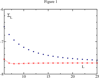
Figure 1: Convergence of the angular-momentum summation. $\alpha=0.9$,$\beta=1$; dots: $\Sigma_{L}$; dashed line with crosses: $\Sigma_{L}^{\rm as}$.

The expressions for the Green’s function and for the one-loop action imply summation over angular momentum $l$. After renormalization these converge in the expected form, the single terms being proportional to $l^{-3}$, while the unsubtracted terms behave like $l^{-1}$. This has been verified numerically and presents a cross check on the procedure and the accuracy. We have appended the sum from $L=l_{\rm max}$ to $\infty$ by adding this sum in its asymptotic form. We have used a fit $A/l^{3}+B/l^{4}+C/l^{5}$ through the five values of $J_{l}$ at $l_{\rm max}-5,\dots,l_{\rm max}$ in order to parameterize the terms in this asymptotic sum. In order to illustrate the convergence in $l$ we plot, in Fig. 1, the values $\Sigma_{L}$ and of $\Sigma_{L}^{\rm as}$, where the latter is the exact finite sum up to $L$ complemented by the asymptotic sum, for $\lambda=0.9,\eta=0.5$. The convergence is seen to be excellent. In our actual calculations we used $l_{\rm max}=25$. The same procedure was applied to the summation over angular momenta occuring in $G(\vec{x},\vec{x})$.

9 Numerical results

The computational framework introduced in the previous sections has been carried through for a representative part of the parameter space. The parameter space is conveniently analyzed [45, 10] in terms of two dimensionless variables $\alpha$ and $\beta$ which are introduced as follows: We define the scaled variables: $X=mx$ and $\Phi=2\eta/m^{2}\phi$. Then the classical action takes the form

$$S_{\rm cl} = \frac{m^{4}}{4\eta^{2}}\int d^{2}X\left[\frac{1}{2}\left(\nabla_{X}\Phi\right)^{2}+\frac{1}{2}\Phi^{2}-\frac{1}{2}\Phi^{3}+\frac{\alpha}{8}\Phi^{4}\right]$$ (9.1)

$$= \beta\hat{S}_{\rm cl}(\alpha)\;,$$

with $\beta=m^{4}/4\eta^{2}$ and $\alpha=\lambda\beta/m^{2}$. The variable $\alpha$ can take values $0<\alpha<1$ as a condition for the existence of the classical bounce solution. $\alpha=1$ corresponds to degenerate minima, the limit $\alpha\to 1$ is called the thin-wall limit. This defines the parameter range for $\alpha$. $\beta$ appears in front of the rescaled classical action while there is no such factor in front of the quantum action which in the one-loop approximation only depends on $\alpha$. Therefore large $\beta$ imply a large classical action and therefore relatively small quantum corrections, small values of $\beta$ make the classical action small and the quantum corrections relatively important. This consideration applies to the one-loop approximation; for a self-consistent scheme the separation of classical and quantum parts is not unique, but this consideration may still serve as an estimate. Indeed we find that for $\beta\lesssim 0.8$ the Hartree iteration, even with an underrelaxation parameter, does not converge.

The computations were started with the one-loop approximation and then iterated until the largest difference in the profiles $\phi(r)$ between two subsequent iterations $\max_{r}\Delta\phi(r)$ was smaller than $10^{-5}$. The convergence of the profiles $\phi(r)$ and of the potential $V(r)$ is displayed in Figs. 2(a) and (b), respectively, for the case $\alpha=0.9,\beta=1$.

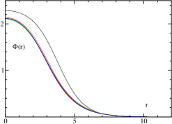
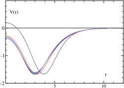
Figure 2: Convergence of the bounce profiles and of the potential for $\alpha=0.9$ and $\beta=1$.

The iteration is found to converge for $\alpha\lesssim 0.9$ and $\beta\gtrsim 0.8$. The translation zero mode is found at typically $|\nu^{2}|\simeq 10^{-4}$ in the one-loop approximation, thus verifying to good accuracy the quality of the classical profile and of the integration of the mode equation. In the Hartree approximation the mode which we continue to identify with the zero mode is located at values of $|\nu^{2}|\simeq 10^{-2}$, the largest value of $0.1$ occurs for $\alpha=0.2,\beta=0.8$. For $\alpha=0.9$ and $\beta=1$ the required accuracy is obtained after $80$ iterations, this takes about $40$ seconds with a $1.3$ GHz processor. For $\alpha<0.9$ and $\beta>1$ the convergence is much faster.

The $\alpha$-dependence of the unstable mode in the one-loop approximation is displayed in Fig. 3. One sees that it approaches zero for $\alpha\to 1$. This is obviously the cause of the lack of convergence for $\alpha>0.9$. During the iteration towards the self-consistent Hartree solution, the mode moves between positive and negative values of $\nu^{2}$ while giving large contributions to ${\rm tr}{\cal G}$. If we look, see Fig. 4, at the effective actions found in the Hartree approximation then there is no evidence of any singular behaviour near $\alpha=0.9$. So we think that the lack of convergence is just a technical problem which could be overcome, but this certainly would need some new analytic idea, not just plain numeric efforts.

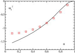
Figure 3: The unstable mode for $\beta=1$. Straight line: one-loop approximation; squares: Hartree approximation.

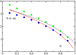
Figure 4: Classical and total actions as functions of $\alpha$, multiplied by $(1-\alpha)$. Dashed line: $S_{\rm cl}^{1-{\rm loop}}$; empty square: thin wall limit of $S_{\rm cl}^{1-{\rm loop}}$; straight line: $S_{\rm tot}^{1-{\rm loop}}$; full squares: $S_{\rm cl}^{\rm Hartree}$; full circles: $S_{\rm tot}^{\rm Hartree}$.

The dependence on the parameter $\alpha$ at fixed $\beta$ is displayed in Fig. 4. The classical actions and the quantum actions in the one-loop and in the Hartree approximations are plotted including a factor $(1-\alpha)$. Indeed all of them are singular in the thin-wall limit $\alpha\to 1$. For the classical action in the one-loop approximation the behavior can be determined analytically using the standard technique (see e.g. [9]) as

$$\lim_{\alpha\to 1}S_{\rm cl}^{1-{\rm loop}}(1-\alpha)=\beta\frac{2\pi}{9}\;.$$ (9.2)

The one loop results extend to $\alpha=0.97$, for the Hartree results we were not able to obtain convergence beyond $\alpha\gtrsim 0.9$ as already mentioned.

(a)         
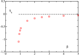
(b)         
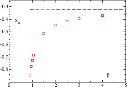
(c)         

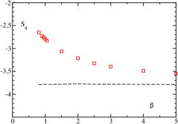
Figure 5: Quantum parts of the effective action as functions of $\beta$. Dashed lines: one-loop approximation; squares: Hartree approximation; (a): $\alpha=0.2$; (b): $\alpha=0.5$; (c): $\alpha=0.9$.

In Figs. 5(a-c) we plot the quantum actions

$$S_{\rm q}^{1-\rm{loop}}=\frac{1}{2}{\ln\det}^{\prime}\frac{-\Delta_{2}+{\cal M}^{2}}{-\Delta_{2}+m^{2}}\;,$$ (9.3)

as obtained in the one-loop approximation and

$$S_{\rm q}^{\rm Hartree}=\frac{1}{2}{\ln\det}^{\prime}\frac{-\Delta_{2}+{\cal M}^{2}}{-\Delta_{2}+m^{2}}-\frac{3\lambda}{8}\int d^{2}x\Delta^{2}(\vec{x})\;,$$ (9.4)

obtained in the Hartree approximation as functions of $\beta$. It is found that the one-loop action, which is independent of $\beta$, and $S_{\rm q}^{\rm Hartree}$ approach each other for large values of $\beta$. When $\beta$ decreases below $\beta=1$ the difference increases rapidly, pointing, for $\alpha=0.2$ and $0.5$, to a kind of singularity at values of $\beta$ between $0.8$ and $0.9$. Below this range the iteration ceases to converge. During the iteration the value of $\phi(0)$ decreases, and the classical profile displays a minimum at some finite value of $r$. The lack of convergence for $\beta\lesssim 0.8$ is not well-understood. For some parameter sets, e.g., $\alpha=0.5$, Fig. 5(b), there seems to be a kind of singularity of the quantum action, which, however, is compensated by an opposite behavior in the classical action, so that is not apparent in their sum, as can be seen in Fig.6(a). Some analytic idea, like reshuffling contributions between the quantum and classical parts, could possibly cure the problem. Indeed in a self-consistent scheme there is no real “classical” part, as the profile depends on the quantum corrections.

(a)         
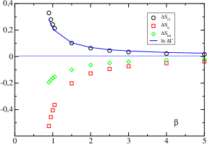
(b)         

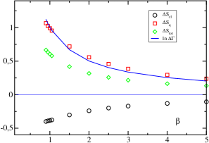
Figure 6: Differences between one-loop and Hartree approximation of various parts of the effective action as functions of $\beta$. Notations as specified in the text; (a): $\alpha=0.5$; (b): $\alpha=0.9$.

In Figs. 6(a,b) we display the difference between the one-loop and the Hartree approximations for various quantities, for $\alpha=0.5$ and $\alpha=0.9$. $\Delta S_{\rm q}=S_{\rm q}^{\rm Hartree}-S_{\rm q}^{1-\rm{loop}}$, the difference of the quantum actions, is found to be negative for $\alpha=0.5$ (and also for $\alpha=0.2$), but positive for $\alpha=0.9$. We also display the difference between the classical actions $\Delta S_{\rm cl}=S_{\rm cl}^{\rm Hartree}-S_{\rm cl}^{1-{\rm loop}}$ and the total difference $\Delta S_{\rm tot}=\Delta S_{\rm cl}+\Delta S_{\rm q}$. We see that even this total difference has different signs for $\alpha=0.5$ and $\alpha=0.9$. We should keep in mind again that the separation between classical and quantum action is not unique and that the classical profile, and therefore the prefactor, depends on the quantum fluctuations. The total width, which includes in the prefactor the normalization of the zero mode is for all $\alpha$ found to be suppressed in the Hartree approximation with respect to the one-loop approximation. This is also displayed in Figs. 6(a) and (b), where the solid line represents

$$\Delta\log\Gamma=-\log\frac{\Gamma^{\rm Hartree}}{\Gamma^{1-{\rm loop}}}\;,$$ (9.5)

with the one-loop transition rate given by Eq. (1.1), and rate in the Hartree approximation given by Eq. (4.2). This difference is positive for both $\alpha=0.5$ and $\alpha=0.9$. These rates are displayed separately in Fig. 7.

We have mentioned above that for the transition rates we use the normalization of the translation mode as prefactor, as the virial theorem used in the one-loop approximation is no longer valid in the Hartree approximation. In the one-loop approximation the normalization of the zero mode and the classical action agree better than four significant digits, in the Hartree approximation the classical and total actions approach the normalization of the zero mode for large $\beta$, but $\beta\simeq 1$ both of them differ from it by factors up to $3$.

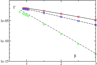
Figure 7: The transition rates in the one-loop and Hartree approximations as functions of $\beta$. One-loop approximation: straight line: $\alpha=0.2$; dashed line: $\alpha=0.5$; dash-dotted line: $\alpha=0.9$; Hartree results: circles: $\alpha=0.2$; squares: $\alpha=0.5$; diamonds: $\alpha=0.9$.

As we have mentioned above the procedure becomes unstable for $\beta\lesssim 1$; the iteration ceases to converge. Bergner and Bettencourt [22], on the other hand present results for $m=1.3469$, and, in our conventions $\lambda=2$ and $\eta=0.9685$. They use the same renormalization convention as we do. Their parameters correspond to $\alpha=0.967$ and $\beta=0.877$. This is close to the thin wall limit, and at a value of $\beta$ for which our procedure to becomes unreliable. The features of the solution found in Ref. [22] are quite different from those found here: there the eigenvalue spectrum displays neither a zero nor an unstable mode. It may be that the tunnelling in this region, $\beta\lesssim 0.9,\alpha>0.9$ takes place in a qualitatively different way. If this is so then our procedure certainly breaks down on more than numerical reasons as it is based on an conventional treatment of zero and unstable modes. In order to obtain a comparison of the result of Ref. [22] with ours, we have determined the various actions for $\beta=0.877$ and $m=1.3469$ fixed, as a function of $\alpha$. These results are plotted in Fig. 8. The classical action of Ref.. [22] agrees reasonably well with our results. We also show the thin wall limit, Eq. (9.2). The total one-loop action can be computed up to $\alpha=0.98$. The total one-loop action obtained in Ref. [22] is somewhat lower than our values. Surprisingly our results for the Hartree approximation seem to extrapolate quite naturally towards the result of Ref.[22].

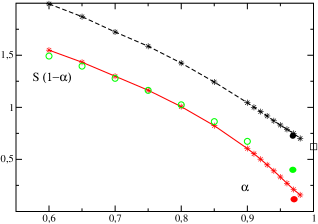
Figure 8: Comparison with Ref. [22]: Dashed line with stars: our results for $S_{\rm cl}^{1-{\rm loop}}$; full line with stars: our results for $S_{\rm tot}^{1-{\rm loop}}$; empty circles: our results for $S^{\rm H}_{\rm tot}$; full circles: the corresponding results of Ref. [22]; empty square: thin wall limit of the classical action; all actions are multiplied with $(1-\alpha)$.

10 Conclusions and outlook

We have presented here a calculation of the transition rate for the false vacuum decay in $(1+1)$ dimensions in the Hartree approximation. We have used analytic and numerical methods that have been applied previously to other systems, for the computations of functional determinants [10, 16, 26] and zero point energies [16, 29]. Both techniques are based on mode functions of the fluctuation operator at $\nu^{2}=0$, as they appear in the standard representation of Green’s functions. Here these techniques are used for the first time in conjunction; as one sees this leads to a rather simple and effective computation scheme with various cross checks. We should like to add, that these techniques are well-suited for coupled-channel systems as well [12]. Renormalization can be dealt with in exact correspondence to standard perturbation theory; this feature extends to applications in higher space-time dimensions and, allowing for dimensional regularization, to computations in gauge theories.

We have presented results for a substantial part of parameter space, using the parameters $\beta=m^{4}/4\eta^{2}$ and $\alpha=\lambda\beta/m^{2}$. Bounces exist only for $\alpha<1$, $\alpha=1$ being the thin wall limit. The second parameter $\beta$ weighs the ratio between classical and quantum contributions to the effective action. We find that for $\beta\gtrsim 0.8$, and for $\alpha\lesssim 0.9$ our iterative determination of the field configuration in the Hartree approximation converges. The unstable mode and an almost-zero mode in the $p$-wave, identified as the translation mode, persist during the iteration and are handled as in the one-loop approximation. We find that the transition rates are generally suppressed in the Hartree approximation, as compared to the one-loop rates. However the corrections are relatively small, less than an order of magnitude. This has been found similarly for the one-loop quantum corrections for instanton transitions in the two-dimensional Abelian Higgs model [11] and may be an general feature of two-dimensional models.

The only similar computation which is available at present is the one of Ref. [22]. Unfortunately our procedure does not converge for the parameters chosen by these authors, which in our convention are $\alpha=0.967$ and $\beta=0.877$. Their self-consistent configuration is qualitatively different from ours in that the fluctuation operator has no unstable and translation modes. If this is the case in this part of the parameter space then it means that the tunneling proceeds in a qualitatively different way, there. Nevertheless we have found that our Hartree results seem to extrapolate naturally towards the ones of Ref. [22].

The methods used here for the computation of self-consistent solutions for bounces naturally extends to bounces in higher space dimensions and to other classical solutions in quantum field theory. In particular, the techniques for covariant regularization and renormalization are available [16, 10] in the framework we have established here.

11 Acknowledgments

N. K. was supported by the Deutsche Forschungsgemeinschaft as a member of Graduiertenkolleg 841.

References

- [1] I. Y. Kobzarev, L. B. Okun and M. B. Voloshin, Sov. J. Nucl. Phys. 20, 644 (1975).
- [2] S. R. Coleman, Phys. Rev. D15, 2929 (1977).
- [3] J. Callan, Curtis G. and S. R. Coleman, Phys. Rev. D16, 1762 (1977).
- [4] S. R. Coleman and F. De Luccia, Phys. Rev. D21, 3305 (1980).
- [5] A. D. Linde, Nucl. Phys. B216, 421 (1983).
- [6] J. S. Langer, Ann. Phys. 54, 258 (1969).
- [7] J. S. Langer, Ann. Phys. 41, 108 (1967).
- [8] I. Affleck, Phys. Rev. Lett. 46, 388 (1981).
- [9] S. Coleman, Aspects of Symmetry (Cambridge University Press, 1985).
- [10] J. Baacke and V. G. Kiselev, Phys. Rev. D48, 5648 (1993), [hep-ph/9308273].
- [11] J. Baacke and T. Daiber, Phys. Rev. D51, 795 (1995), [hep-th/9408010].
- [12] J. Baacke, Phys. Rev. D52, 6760 (1995), [hep-ph/9503350].
- [13] A. Strumia, N. Tetradis and C. Wetterich, Phys. Lett. B467, 279 (1999), [hep-ph/9808263].
- [14] G. Munster and S. Rotsch, Eur. Phys. J. C12, 161 (2000), [cond-mat/9908246].
- [15] G. Munster, A. Strumia and N. Tetradis, Phys. Lett. A271, 80 (2000), [cond-mat/0002278].
- [16] J. Baacke, Z. Phys. C53, 402 (1992).
- [17] N. Graham, R. L. Jaffe and H. Weigel, Int. J. Mod. Phys. A17, 846 (2002), [hep-th/0201148].
- [18] N. Graham et al., Nucl. Phys. B645, 49 (2002), [hep-th/0207120].
- [19] N. Graham et al., Phys. Lett. B572, 196 (2003), [hep-th/0207205].
- [20] A. Surig, Phys. Rev. D57, 5049 (1998), [hep-ph/9706259].
- [21] D. Bodeker, W. Buchmuller, Z. Fodor and T. Helbig, Nucl. Phys. B423, 171 (1994), [hep-ph/9311346].
- [22] Y. Bergner and L. M. A. Bettencourt, Phys. Rev. D69, 045012 (2004), [hep-ph/0308107].
- [23] J. M. Cornwall, R. Jackiw and E. Tomboulis, Phys. Rev. D10, 2428 (1974).
- [24] H. Verschelde and M. Coppens, Phys. Lett. B287, 133 (1992).
- [25] M. Coppens and H. Verschelde, Z. Phys. C58, 319 (1993).
- [26] J. Baacke and G. Lavrelashvili, Phys. Rev. D69, 025009 (2004), [hep-th/0307202].
- [27] C. V. Christov et al., Prog. Part. Nucl. Phys. 37, 91 (1996), [hep-ph/9604441].
- [28] R. Alkofer, H. Reinhardt and H. Weigel, Phys. Rept. 265, 139 (1996), [hep-ph/9501213].
- [29] J. Baacke and H. Sprenger, Phys. Rev. D60, 054017 (1999), [hep-ph/9809428].
- [30] J. Baacke and H. Sprenger, Phys. Rev. D63, 094016 (2001), [hep-ph/0011204].
- [31] A. Okopinska, Phys. Lett. B375, 213 (1996), [hep-th/9508087].
- [32] S. Chiku and T. Hatsuda, Phys. Rev. D58, 076001 (1998), [hep-ph/9803226].
- [33] Y. Nemoto, K. Naito and M. Oka, Eur. Phys. J. A9, 245 (2000), [hep-ph/9911431].
- [34] E. Tomboulis, Phys. Rev. D12, 1678 (1975).
- [35] N. H. Christ and T. D. Lee, Phys. Rev. D12, 1606 (1975).
- [36] J.-L. Gervais and B. Sakita, Phys. Rev. D11, 2943 (1975).
- [37] J.-L. Gervais, A. Jevicki and B. Sakita, Phys. Rev. D12, 1038 (1975).
- [38] J. Baacke and H. J. Rothe, Nucl. Phys. B118, 371 (1977).
- [39] J. Baacke and R. Koch, Nucl. Phys. B135, 304 (1978).
- [40] H. J. de Vega, Nucl. Phys. B115, 411 (1976).
- [41] J. Verwaest, Nucl. Phys. B123, 100 (1977).
- [42] R. F. Dashen, B. Hasslacher and A. Neveu, Phys. Rev. D10, 4114 (1974).
- [43] H. Verschelde, Phys. Lett. B497, 165 (2001), [hep-th/0009123].
- [44] J. Baacke, Acta Phys. Polon. B22, 127 (1991).
- [45] M. Dine, R. G. Leigh, P. Y. Huet, A. D. Linde and D. A. Linde, Phys. Rev. D46, 550 (1992), [hep-ph/9203203].