UPR-1097-T
The Spectra of Heterotic Standard Model Vacua

A formalism for determining the massless spectrum of a class of realistic heterotic string vacua is presented. These vacua, which consist of $SU(5)$ holomorphic bundles on torus-fibered Calabi-Yau threefolds with fundamental group $\mathbb{Z}_{2}$, lead to low energy theories with standard model gauge group $(SU(3)_{C}\times SU(2)_{L}\times U(1)_{Y})/\mathbb{Z}_{6}$ and three families of quarks and leptons. A methodology for determining the sheaf cohomology of these bundles and the representation of $\mathbb{Z}_{2}$ on each cohomology group is given. Combining these results with the action of a $\mathbb{Z}_{2}$ Wilson line, we compute, tabulate and discuss the massless spectrum.

1 Introduction

The early discussions of realistic vacua in heterotic superstring theory were within the context of the “standard embedding” [1] of the spin connection into the gauge connection. Said differently, these vacua always involve a holomorphic $E_{8}$ vector bundle, $V$, which is induced by the tangent bundle $TX$ of the smooth Calabi-Yau threefold $X$. Although leading to interesting low energy physics, this approach suffers from the fact that it is highly constrained, the tangent bundle being only one out of an enormous number of possible holomorphic bundles $V$. One consequence of this constraint is the fact that all heterotic vacua based on the standard embedding require the spontaneous breaking of $E_{8}$ to $E_{6}$, which is then further broken by Wilson lines. Although $E_{6}$ is a possible grand unified group, other groups, such as $SU(5)$ or $Spin(10)$, are simple and more compelling given recent experimental data. Equally significant is that, in the standard embedding, the low energy spectrum and couplings are completely determined by the cohomology of the tangent bundle $TX$. This seriously constrains these quantities, and it has been difficult to find realistic models in this context.

A technical breakthrough in this regard was presented in [2, 3, 4], where it was shown how to construct a large class of stable, holomorphic vector bundles on simply connected elliptically fibered Calabi-Yau threefolds where $V\neq TX$. Such bundles admit connections satisfying the hermitian Yang-Mills equations. This work was extended in [5]-[13], and it was shown that these bundles can lead to heterotic string vacua with a wide range of low energy gauge groups, including $SU(5)$ and $Spin(10)$. Many of the physical properties of these vacua have been studied, including supersymmetry breaking [14, 15], the moduli space of the vector bundle [16]-[19], and, in the strongly coupled case, the associated M5-brane moduli space [20], small instanton phase transitions [21]-[24], non-perturbative superpotentials [16, 25, 26, 27], and fluxes [28]-[34]. More recently, it was shown how to compute the sheaf cohomology of $V$ and its tensor products, thus determining the complete particle physics spectrum [35, 36]. An important conclusion of these papers is that the spectrum depends on the region of vector bundle moduli space in which it is evaluated. Although constant for generic moduli, the spectrum can jump dramatically on subspaces of co-dimension one or higher always containing, however, three families of quarks and leptons. These vacua also underlie the theory of brane universes [6]-[12] and ekpyrotic and Big Crunch/Big Bang cosmology [37]-[40]. The major drawback of these vacua is that the compactification manifold is simply connected. It follows that these are all GUT theories which cannot be broken to the standard model with Wilson lines [41]-[47]. Although many of these vacua contain Higgs multiplets whose vacuum expectation values could induce symmetry breaking, it would be simpler and more natural if Wilson lines could be introduced.

This was accomplished in [48]-[51], where stable holomorphic vector bundles with structure group $SU(5)$ were constructed over torus-fibered Calabi-Yau threefolds with fundamental group $\pi_{1}(X)=\mathbb{Z}_{2}$. These heterotic vacua lead, using a $\mathbb{Z}_{2}$ Wilson line, to low energy theories that are anomaly free, have three families of quarks/leptons and the gauge group $(SU(3)_{C}\times SU(2)_{L}\times U(1)_{Y})/\mathbb{Z}_{6}$. This work was extended to vector bundles with structure group $SU(4)$ on torus-fibered Calabi-Yau threefolds with $\pi_{1}(X)=\mathbb{Z}_{2}\times\mathbb{Z}_{2}$ in [52]-[54] and $\pi_{1}(X)=\mathbb{Z}_{3}\times\mathbb{Z}_{3}$ in [55]. Although very promising, it is essential that one now compute the exact spectrum and couplings in these standard model vacua. In this paper, we take a major step in this direction by computing the particle spectrum for the vacua in [48]-[51].

This is accomplished as follows. In [48]-[51], $X$ is the quotient $X=\tilde{X}/\mathbb{Z}_{2}$, where $\tilde{X}$ is a simply connected Calabi-Yau threefold. Denote by $\tilde{V}$ the pull-back of $V$ to $\tilde{V}$. To find the particle spectrum, one must first compute the sheaf cohomology of $\tilde{V}$ and its tensor products. This is a non-trivial task involving various techniques in cohomological algebra and algebraic geometry. In this paper, we present a systematic approach to such computations, and determine all relevant cohomology groups in our theory. The next step is to find the explicit representations of $\mathbb{Z}_{2}$ in each of these spaces. We give a precise methodology for accomplishing this. This approach is then used to determine each of the requisite $\mathbb{Z}_{2}$ representations. The above information, in conjunction with the action of the $\mathbb{Z}_{2}$ Wilson line, can be utilized to find all group multiplets that are invariant under $\mathbb{Z}_{2}$, as well as their multiplicities. When constructing the quotient Calabi-Yau threefold $X=\tilde{X}/\mathbb{Z}_{2}$, these invariant multiplets descend to $X$ and form the massless particle physics spectrum. Using these techniques, we compute and tabulate the spectrum.

Specifically, we do the following. In Section 2, we present a general formalism for describing $G(\subset E_{8})$-bundles, Wilson lines and the massless spectrum associated with non-simply connected Calabi-Yau threefolds $X$ with $\pi_{1}(X)=F$. It is shown that determining this spectrum requires the computation of specific sheaf cohomologies on the covering Calabi-Yau threefold $\tilde{X}$, as well as the action of $F$ on these groups. This formalism is illustrated for several values of $F$, including $F=\mathbb{Z}_{2}$. Section 3 is devoted to a brief review of the results in [48]-[51]. Specifically, we discuss the construction of torus-fibered Calabi-Yau threefolds $X$ with fundamental group $F=\mathbb{Z}_{2}$. It is shown how to construct stable, holomorphic bundles $V$ with structure group $SU(5)$ on $X$. These arise from $\mathbb{Z}_{2}$ invariant bundles $\tilde{V}$ on $\tilde{X}$ and satisfy the basic phenomenological constraints of particle physics. Computing the massless spectrum of this theory requires determining the sheaf cohomology of $\tilde{V}$ and its tensor products. A general method for doing this is presented in Section 4 and used to compute the relevant cohomology groups in our theory. Section 5 is devoted to finding the explicit representations of $\mathbb{Z}_{2}$ on these cohomology groups. Combining the results of Section 5 with the $F=\mathbb{Z}_{2}$ example in Section 2, the massless spectrum of our theory is computed, tabulated and discussed in Section 5. Finally, in the Appendix we present some useful mathematical facts used throughout the paper.

2 The Spectra of Heterotic Compactifications
with Wilson Lines

A vacuum in weakly coupled heterotic string theory is specified by a pair $(X,\overline{{\mathcal{V}}})$, where $X$ is a Calabi-Yau threefold and $\overline{{\mathcal{V}}}$ is a stable $E_{8}\times E_{8}$ holomorphic principal bundle on $X$ satisfying the Green-Schwarz anomaly cancellation condition [56]

$$c_{2}(\overline{{\mathcal{V}}})=c_{2}(TX)\ .$$ (1)

Note that specifying the $E_{8}\times E_{8}$ bundle $\overline{{\mathcal{V}}}$ is the same as giving two $E_{8}$ bundles ${\mathcal{V}}$ and ${\mathcal{V}}^{\prime\prime}$. The anomaly cancellation condition can be written as

$$c_{2}({\mathcal{V}})+c_{2}({\mathcal{V}}^{\prime\prime})=c_{2}(TX)\ .$$ (2)

In this work, we will always take ${\mathcal{V}}^{\prime\prime}$ to be trivial. Then, condition (2) becomes

$$c_{2}({\mathcal{V}})=c_{2}(TX)\ .$$ (3)

In heterotic M-theory compactifications, this condition is relaxed to

$$c_{2}({\mathcal{V}})+[C]=c_{2}(TX)\ ,$$ (4)

where ${\mathcal{V}}$ is a stable holomorphic $E_{8}$ principal bundle in the observable sector and $[C]$ is the class of some effective curve $C\subset X$ on which M5-branes wrap.

The particle spectrum of this compactification consists [1] of zero-modes of the ten-dimensional Dirac operator

$$/{\!\!\!\!D}:\Gamma({\mathop{\rm ad}}{\mathcal{V}}\otimes S^{+}_{10})\rightarrow\Gamma({\mathop{\rm ad}}{\mathcal{V}}\otimes S^{-}_{10})\ .$$ (5)

Here ${\mathop{\rm ad}}{\mathcal{V}}$ is the rank-248 vector bundle associated to ${\mathcal{V}}$ by the adjoint representation of $E_{8}$, $S^{\pm}_{10}$ are the bundles of positive and negative chirality spinors in 10-dimensions, and $\Gamma$ denotes global sections of a bundle over the 10-dimensional space $\mathbb{R}^{4}\times X$. (Note that we can consider ${\mathop{\rm ad}}{\mathcal{V}}$ to be a bundle on $\mathbb{R}^{4}\times X$ by simply pulling it back from $X$).

The 10-dimensional spinors decompose in terms of their (Minkowski) $\mathbb{R}^{4}$ and (internal) $X$ components as

$$S^{+}_{10}=(S^{+}_{4}\otimes S^{+}_{6})\oplus(S^{-}_{4}\otimes S^{-}_{6}).$$ (6)

The internal spinors, on the Calabi-Yau threefold $X$, can be identified with the $(0,q)$ forms ${\cal A}^{0,q}$ on $X$, with even/odd $q$ corresponding to positive/negative chirality:

$$S^{+}_{6}\simeq{\cal A}^{0,0}\oplus{\cal A}^{0,2},\qquad S^{-}_{6}\simeq{\cal A}^{0,1}\oplus{\cal A}^{0,3}.$$ (7)

In terms of this identification, the Dirac operator becomes $/{\!\!\!\!D}=\overline{\partial}+\overline{\partial}^{*}+/{\!\!\!\!D}_{4}$ coupled to ${\mathop{\rm ad}}{\mathcal{V}}$, where $\overline{\partial}$ is the Dolbeault operator on $X$, and $/{\!\!\!\!D}_{4}$ is the Dirac operator on flat $\mathbb{R}^{4}$. Putting these facts together, we find that the spectrum is

$$\ker(/{\!\!\!\!D})\simeq\left(\bigoplus_{q=0,2}H^{q}(X,{\mathop{\rm ad}}{\mathcal{V}})\otimes{\bf S}^{+}_{4}\right)\oplus\left(\bigoplus_{q=1,3}H^{q}(X,{\mathop{\rm ad}}{\mathcal{V}})\otimes{\bf S}^{-}_{4}\right),$$ (8)

where ${\bf S}^{\pm}_{4}$ denote the constant sections of the bundle $S^{\pm}_{4}$ on $\mathbb{R}^{4}$. The positive chirality particles are those which multiply ${\bf S}^{+}_{4}$, so they are given by (a basis of)

$$\bigoplus_{q=0,2}H^{q}(X,{\mathop{\rm ad}}{\mathcal{V}}).$$ (9)

Their negative chirality anti-particles are similarly given by a basis of

$$\bigoplus_{q=1,3}H^{q}(X,{\mathop{\rm ad}}{\mathcal{V}}).$$ (10)

By Serre duality, this is the dual space to (9), as it should be by CPT. Recall that, for each charged particle, CPT predicts the existence of an anti-particle of opposite charge. The annihilation of a particle with its anti-particle can be interpreted as a natural pairing. Hence, we can interpret the space of anti-particles as the dual of the space of particles. In order to describe the complete spectrum, we will in this work calculate

$$Spec:=\bigoplus_{q=0,1}H^{q}(X,{\mathop{\rm ad}}{\mathcal{V}}).$$ (11)

Then, $\ker(/{\!\!\!\!D})$ is obtained by adding the duals to $Spec$.

In practice, the $E_{8}$ bundle ${\mathcal{V}}$ is often associated to some stable $G$-bundle $V$ on $X$, where $G\subset E_{8}$ is some subgroup, e.g., $G=SU(n)$ for $n=3,4$ or $5$ :

$${\mathcal{V}}=V\stackrel{{\scriptstyle G}}{{\times}}E_{8}\ .$$ (12)

The resulting compactification then has a low energy gauge group

$$H=Z_{E_{8}}(G)\ ,$$ (13)

the commutant of $G$ in $E_{8}$. The decomposition of the 248-dimensional representation ${\mathop{\rm ad}}E_{8}$ under the product $G\times H$ then gives an associated decomposition for ${\mathop{\rm ad}}{\mathcal{V}}$ and the Dirac-operator zero-modes. For example, we can take $V$ to be an $SU(3)$ bundle, or equivalently, a rank 3 vector bundle with trivial determinant. The usual embedding of $G=SU(3)$ into $E_{8}$ has commutant $H=E_{6}$. The decompostion of ${\mathop{\rm ad}}E_{8}$ into irreducible representations of $SU(3)\times E_{6}$ involves four terms

$$248=(1,78)\oplus(8,1)\oplus(3,27)\oplus(\overline{3},\overline{27})\ .$$ (14)

Here, 8 and 78 are the adjoints of $SU(3)$ and $E_{6}$ respectively, 3 is the fundamental representation of $SU(3)$, and 27, $\overline{27}$ are the smallest representations of $E_{6}$. For the zero-modes we get:

$$Spec=\left(H^{0}(X,{\mathcal{O}}_{X})\otimes 78\right)\oplus\left(H^{1}(X,{\mathop{\rm ad}}V)\otimes{\hbox to0.0pt{1\hss}\hskip 1.6pt\hbox{1}}\right)\oplus\left(H^{1}(X,V)\otimes 27\right)\oplus\left(H^{1}(X,V^{*})\otimes\overline{27}\right)\ .$$ (15)

Here we think of $V$ as a rank 3 vector bundle on $X$ associated to the principal $SU(3)$ bundle by the fundamental representation, $V^{*}$ is its dual vector bundle, ${\mathop{\rm ad}}V$ is the rank-8 vector bundle of traceless endomorphisms of $V$, and ${\mathcal{O}}_{X}$ is the trivial rank-1 bundle on $X$. Note that the stability of $V$ and the Calabi-Yau property of $X$ guarantee that for each of the associated bundles $({\mathcal{O}}_{X},{\mathop{\rm ad}}V,V,V^{*})$, the cohomology can be non-zero for either $q=0$ or $q=1$ but not both, as indicated in (15).

As another example, we consider the usual embedding of $G=SU(5)$ into $E_{8}$. The commutant is $H=SU(5)$ and the $SU(5)_{G}\times SU(5)_{H}$-decomposition is

$$248=(1,24)\oplus(24,1)\oplus(10,5)\oplus(\overline{10},\overline{5})\oplus(5,\overline{10})\oplus(\overline{5},10)\ .$$ (16)

The zero-modes are

$$Spec = \left(H^{0}(X,{\mathcal{O}}_{X})\otimes 24\right)\oplus\left(H^{1}(X,{\mathop{\rm ad}}V)\otimes{\hbox to0.0pt{1\hss}\hskip 1.6pt\hbox{1}}\right)\oplus\left(H^{1}(X,\wedge^{2}V)\otimes 5\right)\oplus\left(H^{1}(X,\wedge^{2}V^{*})\otimes\overline{5}\right)$$ (17)

$$\oplus\left(H^{1}(X,V)\otimes\overline{10}\right)\oplus\left(H^{1}(X,V^{*})\otimes 10\right)\ .$$

More generally, for $G\subset E_{8}$ with commutant $H$, we write

$${\mathop{\rm ad}}E_{8}=\bigoplus_{i}U_{i}\otimes R_{i}\ ,$$ (18)

where $U_{i}$ runs over irreducible representations of $G$, and $R_{i}$ are corresponding representations of $H$. Using this decomposition of the representation ${\mathop{\rm ad}}E_{8}$ on each fiber of the $E_{8}$ bundle defined in (12), we find the decomposition

$${\mathop{\rm ad}}{\mathcal{V}}=\bigoplus_{i}U_{i}(V)\otimes R_{i}\ ,$$ (19)

where $U_{i}(V)$ are the vector bundles associated to the $G$-bundle $V$ via the representations $U_{i}$ of $G$.

Next we want to see how these results are modified by Wilson lines. Let $F\subset H$ be a finite subgroup which acts on a Calabi-Yau threefold $\tilde{X}$ freely with a Calabi-Yau quotient $X=\tilde{X}/F$. The $G$-bundle $V$ and the $E_{8}$-bundle ${\mathcal{V}}=V\stackrel{{\scriptstyle G}}{{\times}}E_{8}$ on $X$ pull back to a $G$-bundle $\tilde{V}=p^{*}V$ and an $E_{8}$-bundle $\tilde{{\mathcal{V}}}=p^{*}{\mathcal{V}}=\tilde{V}\stackrel{{\scriptstyle G}}{{\times}}E_{8}$ on $\tilde{X}$, where $p:\tilde{X}\rightarrow X$ is the covering map. The action of $F$ on $\tilde{X}$ lifts to actions, denoted $\rho$, on $\tilde{V}$, $\tilde{{\mathcal{V}}}$, hence on their cohomologies. The cohomology group computed on $X$ is precisely the $\rho(F)$-invariant part of the cohomology on $\tilde{X}$

$$H^{q}(X,{\mathop{\rm ad}}{\mathcal{V}})=H^{q}(\tilde{X},{\mathop{\rm ad}}\tilde{{\mathcal{V}}})^{\rho(F)}\ .$$ (20)

The Wilson line $W$ is the flat $H$-bundle on $X$ induced from the $F$-cover $p:\tilde{X}\rightarrow X$ via the given embedding of $F$ in $H$:

$$W:=\tilde{X}\stackrel{{\scriptstyle F}}{{\times}}H\ .$$ (21)

The $(G\times H)$-bundle $V\oplus W$ induces another $E_{8}$-bundle on $X$:

$${\mathcal{V}}^{\prime}=(V\oplus W)\stackrel{{\scriptstyle(G\times H)}}{{\times}}E_{8}\ .$$ (22)

Our goal in this work is to study the particle spectrum and other properties of the heterotic vacuum given by compactification on $(X,{\mathcal{V}}^{\prime})$. Since the structure group of ${\mathcal{V}}^{\prime}$ can be reduced to $G\times F$ (but not to $G$), we see in analogy with (13) that this vacuum has low energy gauge group

$$S:=Z_{H}(F)=Z_{E_{8}}(G\times F)\ .$$ (23)

We will work primarily with a particular class of geometric examples which is reviewed in Section 2. In the remainder of the present section we will describe the general approach. This is based on the observation that, when pulled backed to $\tilde{X}$, the two bundles ${\mathcal{V}}$, ${\mathcal{V}}^{\prime}$ coincide:

$$p^{*}{\mathcal{V}}^{\prime}\simeq p^{*}{\mathcal{V}}=\tilde{{\mathcal{V}}}\ .$$ (24)

This is because the finite structure group $F$ of the Wilson line $W$ is killed in the passage from $X$ to $\tilde{X}$. Another way to describe this is to note that there are two actions $\rho$, $\rho^{\prime}$ of $F$ on $\tilde{{\mathcal{V}}}$, both lifting the given $F$ action on $\tilde{X}$. The quotient by $\rho$ gives ${\mathcal{V}}$, and the quotient by $\rho^{\prime}$ gives ${\mathcal{V}}^{\prime}$. The analogue of (20) is:

$$H^{q}(X,{\mathop{\rm ad}}{\mathcal{V}}^{\prime})=H^{q}(\tilde{X},{\mathop{\rm ad}}\tilde{{\mathcal{V}}})^{\rho^{\prime}(F)}\ .$$ (25)

We can write the decomposition (19) on $\tilde{X}$:

$${\mathop{\rm ad}}\tilde{{\mathcal{V}}}=\bigoplus_{i}U_{i}(\tilde{V})\otimes R_{i}$$ (26)

and use formulas (20), (25) to descend to $X$. The $\rho$ action of $F$ acts only on the associated vector bundles $U_{i}(\tilde{V})$, hence on their cohomology, so:

$$H^{q}(X,{\mathop{\rm ad}}{\mathcal{V}})=\bigoplus_{i}H^{q}(\tilde{X},U_{i}(\tilde{V}))^{\rho(F)}\otimes R_{i}\ .$$ (27)

The $\rho^{\prime}$ action of $F$ is a combination of the $\rho$ action on the $U_{i}(\tilde{V})$ with the action of $F\subset H$ on the $R_{i}$:

$$H^{q}(X,{\mathop{\rm ad}}{\mathcal{V}}^{\prime})=\bigoplus_{i}\left(H^{q}(\tilde{X},U_{i}(\tilde{V}))\otimes R_{i}\right)^{\rho^{\prime}(F)}\ .$$ (28)

Recall that $H^{q}(X,{\mathop{\rm ad}}{\mathcal{V}})$ and its decomposition (27) carry an action of $H$ (which is the natural action on $R_{i}$ in (27)), but only the subgroup $S\subset H$ acts on $H^{q}(X,{\mathop{\rm ad}}{\mathcal{V}}^{\prime})$ and its decomposition (28). To make the latter more explicit, we decompose each $H$-representation $R_{i}$ in terms of the irreducible $F$-representations $A_{j}$:

$$R_{i}=\bigoplus_{j}(A_{j}\otimes B_{ij}),\quad B_{ij}:={\rm Hom}_{F}(A_{j},R_{i})\ .$$ (29)

Our formula (28) for the particle spectrum then becomes

$$H^{q}(X,{\mathop{\rm ad}}{\mathcal{V}}^{\prime})=\bigoplus_{i,j}(H^{q}(\tilde{X},U_{i}(\tilde{V}))\otimes A_{j})^{\rho^{\prime}(F)}\otimes B_{ij}\ .$$ (30)

Here each $B_{ij}$ carries a representation of the low energy gauge group $S$, which occurs in $H^{q}(X,{\mathop{\rm ad}}{\mathcal{V}}^{\prime})$ with multiplicity $m_{ij}$ equal to the dimension of the space of $F$-invariants in $H^{q}(\tilde{X},U_{i}(\tilde{V}))\otimes A_{j}$. Note that the $S$-representation $B_{ij}$ is often not irreducible. Rather, we should think of $B_{ij}$ as a block of irreducible $S$-representations, each of which corresponds to some particle. All the particles in a given block $B_{ij}$ occur in the spectrum with the same multiplicity $m_{ij}$.

We can summarize our procedure so far as follows. The input involves

• a structure group $G\subset E_{8}$,

• a finite subgroup $F$ of the commutant $H=Z_{E_{8}}(G)$,

• a free action of $F$ on a Calabi-Yau threefold $\tilde{X}$ with Calabi-Yau quotient $X=\tilde{X}/F$, and

• a $G$-bundle $V$ on $X$ satisfying the anomaly cancellation condition (4).

These data determine a Wilson line $W$ on $X$ (as in (21)) and a heterotic vacuum $(X,{\mathcal{V}}^{\prime})$ where ${\mathcal{V}}^{\prime}$ combines the $G$-bundle $V$ with the Wilson line $W$, as in (22). The low energy gauge group of this vacuum is the subgroup $S\subset H$ given in (23). The particle spectrum is determined as follows:

• Decompose ${\mathop{\rm ad}}E_{8}$ as in (18) in terms of irreducible $G$-representations $U_{i}$ and corresponding $H$-representations $R_{i}$.

• Decompose each $R_{i}$ as in (29) in terms of irreducible $F$-representations $A_{j}$ and corresponding blocks of irreducible $S$-representations $B_{ij}$.

• Most of the work then goes into computing the cohomology groups $H^{q}(\tilde{X},U_{i}(\tilde{V}))$ of the associated vector bundles on $\tilde{X}$, and the action of $F$ on these cohomologies. The multiplicity $m_{ij}$ of the irreducible $F$-representation $A_{j}^{*}$ in $H^{q}(\tilde{X},U_{i}(\tilde{V}))$ is the multiplicity of all particles from block $B_{ij}$ in the particle spectrum of $(X,{\mathcal{V}}^{\prime})$.

We illustrate the general procedure in two cases. First consider $G=SU(3)$, $H=E_{6}$. As we saw in (14), the $U_{i}$ are 1, 8, 3 and $\overline{3}$, and the corresponding $R_{i}$ are 78, 1, 27 and $\overline{27}$. Now $H=E_{6}$ has a maximal subgroup

$$H_{0}=SU(3)_{C}\times SU(3)_{L}\times SU(3)_{R}\ ,$$ (31)

where we can think of $C$, $L$, $R$ as standing for color, left, right. We can, for example, take $F=F(n,\hat{n})=\mathbb{Z}_{n}\times\mathbb{Z}_{\hat{n}}$ whose two generators are mapped to $H_{0}$ as

$${\hbox to0.0pt{1\hss}\hskip 1.6pt\hbox{1}}_{C}\times\left(\matrix{\alpha&&\cr&\alpha&\cr&&\alpha^{-2}}\right)_{L}\times{\hbox to0.0pt{1\hss}\hskip 1.6pt\hbox{1}}_{R}\ ,\qquad\qquad{\hbox to0.0pt{1\hss}\hskip 1.6pt\hbox{1}}_{C}\times{\hbox to0.0pt{1\hss}\hskip 1.6pt\hbox{1}}_{L}\times\left(\matrix{\hat{\alpha}&&\cr&\hat{\alpha}&\cr&&\hat{\alpha}^{-2}}\right)_{R}\ ,$$ (32)

where $\alpha$ and $\hat{\alpha}$ are roots of unity of orders $n$ and $\hat{n}$ respectively. Another possibility is to work with $F_{0}$, the diagonal subgroup $\mathbb{Z}_{n}$ in $F(n,n)$, with generator

$${\hbox to0.0pt{1\hss}\hskip 1.6pt\hbox{1}}_{C}\times\left(\matrix{\alpha&&\cr&\alpha&\cr&&\alpha^{-2}}\right)_{L}\times\left(\matrix{\alpha&&\cr&\alpha&\cr&&\alpha^{-2}}\right)_{R}\ .$$ (33)

Either $F$ (with $n,\hat{n}>1$) or $F_{0}$ (with $n>1$) break $E_{6}$ to

$$S=SU(3)_{C}\times\left(\frac{SU(2)\times U(1)}{\mathbb{Z}_{2}}\right)_{L}\times\left(\frac{SU(2)\times U(1)}{\mathbb{Z}_{2}}\right)_{R}\ .$$ (34)

In this case, it is easier to first decompose each $R_{i}$ under $H_{0}$, and then to further decompose each $H_{0}$ component under $F$ and $S$. Under $H_{0}$ we have:

$$78 = (8,1,1)\oplus(1,8,1)\oplus(1,1,8)\oplus(3,3,3)\oplus(\overline{3},\overline{3},\overline{3})$$

$$1 = (1,1,1)$$

$$27 = (3,\overline{3},1)\oplus(1,3,\overline{3})\oplus(\overline{3},1,3)$$

$$\overline{27} = (\overline{3},3,1)\oplus(1,\overline{3},3)\oplus(3,1,\overline{3})\ ,$$ (35)

where $(a,b,c)$ is shorthand for the $H_{0}$-representation $a_{C}\otimes b_{L}\otimes c_{R}$. When we further decompose under $S$, the color representations are unchanged, while the 3 of $L$ or $R$ breaks as $2_{1}\oplus 1_{-2}$, and the adjoint 8 breaks as $3_{0}\oplus 1_{0}\oplus 2_{3}\oplus 2_{-3}$. (Here $b_{w}$ denotes the $b$-dimensional representation of $SU(2)$, on which $U(1)$ acts with weight $w$. This representation of $SU(2)\times U(1)$ factors through $(SU(2)\times U(1))/\mathbb{Z}_{2}$ if and only if the integers $b$ and $w$ have opposite parity.) So the $(8,1,1)$ of $H_{0}$ becomes $(8,1,1)_{0,0}$ of $S$, while the $(1,8,1)$ becomes $(1,3,1)_{0,0}\oplus(1,1,1)_{0,0}\oplus(1,2,1)_{3,0}\oplus(1,2,1)_{-3,0}$. The two subscripts give the weights of the two $U(1)$’s in $S$. The same subscripts taken modulo $n$ and $\hat{n}$ give the weights of $F(n,\hat{n})$, so they determine the representation $A_{j}$. We tabulate the results in Table 1. In that table, the only reducible block is $B_{00}$. However, if we replace $F$ by its subgroup $F_{0}$, many of the $A_{j}$ coalesce, resulting in many reducible $B_{ij}$’s.

$$\begin{array}[]{||c|c|c|c|c||}\hline\cr\hline\cr U_{i}&H^{q}(\tilde{X},U_{i}(\tilde{V}))&R_{i}&A_{j}&B_{ij}\\ \hline\cr\hline\cr 1&H^{0}(\tilde{X},{\mathcal{O}}_{\tilde{X}})&78&0,0&(8,1,1)\oplus(1,3,1)\oplus(1,1,3)\oplus 2\times(1,1,1)\\ \hline\cr&&&3,0&(1,2,1)\\ \hline\cr&&&-3,0&(1,2,1)\\ \hline\cr&&&0,3&(1,1,2)\\ \hline\cr&&&0,-3&(1,1,2)\\ \hline\cr&&&1,1&(3,2,2)\\ \hline\cr&&&-2,-2&(3,1,1)\\ \hline\cr&&&-1,-1&(\overline{3},2,2)\\ \hline\cr&&&2,2&(\overline{3},1,1)\\ \hline\cr&&&1,-2&(3,2,1)\\ \hline\cr&&&-2,1&(3,1,2)\\ \hline\cr&&&-1,2&(\overline{3},2,1)\\ \hline\cr&&&2,-1&(\overline{3},1,2)\\ \hline\cr 8&H^{1}(\tilde{X},{\mathop{\rm ad}}\tilde{V})&1&0,0&(1,1,1)\\ \hline\cr 3&H^{1}(\tilde{X},\tilde{V})&27&-1,0&(3,2,1)\\ \hline\cr&&&2,0&(3,1,1)\\ \hline\cr&&&1,-1&(1,2,2)\\ \hline\cr&&&-2,-1&(1,1,2)\\ \hline\cr&&&1,2&(1,2,1)\\ \hline\cr&&&-2,2&(1,1,1)\\ \hline\cr&&&0,1&(\overline{3},1,2)\\ \hline\cr&&&0,-2&(\overline{3},1,1)\\ \hline\cr\overline{3}&H^{1}(\tilde{X},\tilde{V^{*}})&\overline{27}&-1,0&(\overline{3},2,1)\\ \hline\cr&&&2,0&(\overline{3},1,1)\\ \hline\cr&&&1,-1&(1,2,2)\\ \hline\cr&&&-2,-1&(1,1,2)\\ \hline\cr&&&1,2&(1,2,1)\\ \hline\cr&&&-2,2&(1,1,1)\\ \hline\cr&&&0,1&(3,1,2)\\ \hline\cr&&&0,-2&(3,1,1)\\ \hline\cr\hline\cr\end{array}$$

Table 1: The decomposition of $H^{q}(X,{\mathop{\rm ad}}{\mathcal{V}}^{\prime})$ where $G=SU(3)$ and $F=\mathbb{Z}_{n}\times\mathbb{Z}_{\hat{n}}$.

For our second example we consider $G=SU(5)$, so $H=SU(5)$ and the decomposition of ${\mathop{\rm ad}}E_{8}$ is given in (16). The finite group $F$ is $\mathbb{Z}_{2}$, where the generator is embedded in $H=SU(5)$ diagonally with eigenvalues $(1,1,1,-1,-1)$. This breaks $H$ to the standard model group $S=(SU(3)_{C}\times SU(2)_{L}\times U(1)_{Y})/\mathbb{Z}_{6}$. In Table 2, we use $(a,b)_{w}$ to denote the product of an $a$-dimensional representation of $SU(3)$ with a $b$-dimensional representation of $SU(2)$, where $U(1)$ acts with weight $w=3Y$. The corresponding representation $A_{j}$ of $F$ depends only on the parity of $w$.

$$\begin{array}[]{||c|c|c|c|c||}\hline\cr\hline\cr U_{i}&H^{q}(\tilde{X},U_{i}(\tilde{V}))&R_{i}&A_{j}&B_{ij}\\ \hline\cr\hline\cr 1&H^{0}(\tilde{X},{\mathcal{O}}_{\tilde{X}})&24&0&(8,1)_{0}\oplus(1,3)_{0}\oplus(1,1)_{0}\\ \hline\cr&&&1&(3,2)_{-5}\oplus(\overline{3},2)_{5}\\ \hline\cr 24&H^{1}(\tilde{X},{\mathop{\rm ad}}\tilde{V})&1&0&(1,1)_{0}\\ \hline\cr 10&H^{1}(\tilde{X},\wedge^{2}\tilde{V})&5&0&(3,1)_{-2}\\ \hline\cr&&&1&(1,2)_{3}\\ \hline\cr\overline{10}&H^{1}(\tilde{X},\wedge^{2}\tilde{V}^{*})&\overline{5}&0&(\overline{3},1)_{2}\\ \hline\cr&&&1&(1,2)_{-3}\\ \hline\cr 5&H^{1}(\tilde{X},\tilde{V})&\overline{10}&0&(3,1)_{4}\oplus(1,1)_{-6}\\ \hline\cr&&&1&(\overline{3},2)_{-1}\\ \hline\cr\overline{5}&H^{1}(\tilde{X},\tilde{V}^{*})&10&0&(\overline{3},1)_{-4}\oplus(1,1)_{6}\\ \hline\cr&&&1&(3,2)_{1}\\ \hline\cr\hline\cr\end{array}$$

Table 2: The decomposition of $H^{q}(X,{\mathop{\rm ad}}{\mathcal{V}}^{\prime})$ where $G=SU(5)$ and $F=\mathbb{Z}_{2}$. The $A_{j}$ correspond to characters of the $\mathbb{Z}_{2}$ action on $R_{i}$. The $a,b$ in $(a,b)_{w}$ are the representations of $SU(3)_{C}$ and $SU(2)_{L}$ respectively, whereas $w=3Y$.

3 Standard Model Bundles

In this section we recall the standard model bundles constructed in [48, 49, 50]. We need a quadruple $(\tilde{X},A,\tau,\tilde{V})$ satisfying:

$$\bullet ({\bf\mathbb{Z}_{2}}) \tilde{X} \tau:\tilde{X}\rightarrow\tilde{X}$$ is a smooth Calabi-Yau 3-fold and is a freely acting involution.

$$A \tilde{X}$$ is a fixed ample line bundle (Kähler structure) on .

$$\bullet {\bf(S)} \tilde{V} A \tilde{X} G=SU(5)$$ is an -stable vector bundle of rank five on with structure group .

$$\bullet {\bf(I)} \tilde{V} \tau$$ is -invariant.

$$\bullet {\bf(C1)} c_{1}(\tilde{V})=0$$ .

$$\bullet {\bf(C2)} c_{2}(\tilde{X})-c_{2}(\tilde{V})$$ is effective.

$$\bullet {\bf(C3)} c_{3}(\tilde{V})=12$$ . (36)

The involution $\tau$ generates a subgroup $\mathbb{Z}_{2}=F\subset H=Z_{E_{8}}(SU(5))=SU(5)$. The quotient $X:=\tilde{X}/F$ is another Calabi-Yau threefold, and invariance of $\tilde{V}$ allows us to identify it with the pullback of a stable $SU(5)$ bundle $V$ on $X$, as in Section 2. This produces a heterotic M-theory vacuum $(X,{\mathcal{V}}^{\prime})$ with particle spectrum as given in Table 2 of Section 2.

3.1 Rational Elliptic Surfaces and Their Products

The simply connected threefold $\tilde{X}$ is a complete intersection in $\mathbb{P}^{1}\times\mathbb{P}^{2}\times(\mathbb{P}^{2})^{\prime}$ of two hypersurfaces of multidegrees $(1,3,0)$ and $(1,0,3)$ respectively. This is a Calabi-Yau, by adjunction, and it has two elliptic fibrations. These threefolds were first studied by Schoen [57]. Choose projective coordinates: $[t_{0}:t_{1}]$ on $\mathbb{P}^{1}$; $z=[z_{0}:z_{1}:z_{2}]$ on $\mathbb{P}^{2}$; and $z^{\prime}=[z_{0}^{\prime}:z_{1}^{\prime}:z_{2}^{\prime}]$ on $(\mathbb{P}^{2})^{\prime}$. The two hypersurfaces can be written:

$$t_{0}f_{0}(z)-t_{1}f_{1}(z) = 0$$ (37)

$$t_{0}f_{0}^{\prime}(z^{\prime})-t_{1}f_{1}^{\prime}(z^{\prime}) = 0\ ,$$ (38)

where $f_{0},f_{1},f_{0}^{\prime},f_{1}^{\prime}$ are homogeneous cubic polynomials. Since equation (37) does not involve $z^{\prime}$, it defines a hypersurface $B\subset\mathbb{P}^{1}\times\mathbb{P}^{2}$. Similarly equation (38) defines a hypersurface $B^{\prime}\subset\mathbb{P}^{1}\times(\mathbb{P}^{2})^{\prime}$. The surfaces $B$, $B^{\prime}$ are called rational elliptic surfaces, or (inaccurately) $dP_{9}$’s. The projections of these surfaces to $\mathbb{P}^{1}$ are elliptic fibrations:

$$\beta:B\rightarrow\mathbb{P}^{1},\qquad\beta^{\prime}:B^{\prime}\rightarrow\mathbb{P}^{1}\ .$$ (39)

The original threefold $\tilde{X}$ comes with the two projections

$$\pi:\tilde{X}\rightarrow B^{\prime},\qquad\pi^{\prime}:\tilde{X}\rightarrow B$$ (40)

which are again elliptic fibrations. In fact, $\tilde{X}$ is the fiber product

$$\tilde{X}=B\times_{\mathbb{P}^{1}}B^{\prime}\ ,$$ (41)

meaning that a point of $\tilde{X}$ is uniquely specified by a pair of points $b\in B$, $b^{\prime}\in B^{\prime}$ with $\beta(b)=\beta^{\prime}(b^{\prime})\in\mathbb{P}^{1}$.

The opposite projection $\nu:B\rightarrow\mathbb{P}^{2}$ is birational, exhibiting $B$ as the blowup of $\mathbb{P}^{2}$ at the 9 points $A_{i}$, $i=1,\ldots,9$ where $f_{0}(z)=f_{1}(z)=0$, and similarly for $B^{\prime}$. (This is the origin of the “$dP_{9}$” name – but these surfaces are not del Pezzos.) It follows that $H^{2}(B,\mathbb{Z})=Pic(B)$ has rank 10. An orthogonal basis consists of the class $\ell:=\nu^{*}{\mathcal{O}}_{\mathbb{P}^{2}}(1)$ together with the 9 exceptional classes $e_{1},\ldots,e_{9}$. The only non-zero intersection numbers on $B$ are $\ell^{2}=1,\quad e_{i}^{2}=-1$, $i=1,\ldots,9$. The class $f:=\beta^{-1}(\mbox{point})$ of an elliptic fiber is given by $f=3\ell-\sum\limits_{i=1}^{9}e_{i}$. There is an analogous basis $\ell^{\prime},e_{1}^{\prime},\ldots,e_{9}^{\prime}$ on $B^{\prime}$. The rank of $H^{2}(\tilde{X},\mathbb{Z})$ is therefore 19, with basis $\pi^{*}\ell^{\prime}=(\pi^{\prime})^{*}\ell,\pi^{*}e_{1}^{\prime},\ldots,\pi^{*}e_{9}^{\prime},(\pi^{\prime})^{*}e_{1},\ldots,(\pi^{\prime})^{*}e_{9}$.

3.2 Special Rational Elliptic Surfaces

In order to obtain the involution $\tau$ on $\tilde{X}$, and also in order to have invariant bundles $\tilde{V}$ on $\tilde{X}$ satisfying the required conditions, the rational elliptic surfaces $B$, $B^{\prime}$ need to be specialized to a particular subfamily. This can be specified as follows.

Let $\Gamma_{1}\subset\mathbb{P}^{2}$ be a nodal cubic with a node $A_{8}$. Choose four generic points on $\Gamma_{1}$ and label them $A_{1},A_{2},A_{3},A_{7}$. Let $\Gamma\subset\mathbb{P}^{2}$ be the unique smooth cubic which passes through $A_{1},A_{2},A_{3},A_{7},A_{8}$ and is tangent to the lines $\langle A_{7}A_{i}\rangle$ for $i=1,2,3$ and $8$. Consider the pencil of cubics spanned by $\Gamma_{1}$ and $\Gamma$. All cubics in this pencil pass through $A_{1},A_{2},A_{3},A_{7},A_{8}$ and are tangent to $\Gamma$ at $A_{8}$. Let $A_{4},A_{5},A_{6}$ be the remaining three base points, and let $B$ denote the blow-up of $\mathbb{P}^{2}$ at the points $A_{i}$, $i=1,2,\ldots,8$ and the point $A_{9}$ which is infinitesimally near $A_{8}$ and corresponds to the line $\langle A_{7}A_{8}\rangle$.

The pencil becomes the anti-canonical map $\beta:B\rightarrow\mathbb{P}^{1}$ which is an elliptic fibration with a section. The map $\beta$ has two reducible fibers $f_{i}=n_{i}\cup o_{i}$, $i=1,2$ of type $I_{2}$. We denote by $e_{i}$, $i=1,\ldots,7$ and $e_{9}$ the exceptional divisors corresponding to $A_{i}$, $i=1,\ldots,7$ and $A_{9}$, and by $e_{8}$ the reducible divisor $e_{9}+n_{1}$. The divisors $e_{i}$ together with the pullback $\ell$ of a class of a line from $\mathbb{P}^{2}$ form a standard basis in $H^{2}(B,{\mathbb{Z}})$.

The surface $B$ has an involution $\alpha_{B}$ which is uniquely characterized by the properties: $\beta\circ\alpha_{B}=\tau_{\mathbb{P}^{1}}\circ\beta$, where $\tau_{\mathbb{P}^{1}}$ is the involution $t_{0}\rightarrow t_{0},t_{1}\rightarrow-t_{1}$ on $\mathbb{P}^{1}$, and $\alpha_{B}$ fixes the proper transform of $\Gamma$ pointwise. Note that $\tau_{\mathbb{P}^{1}}$ leaves two points in $\mathbb{P}^{1}$ fixed, which we call $0$ and $\infty$. Furthermore, $\alpha_{B}$ acts as $(-1)_{B}$ when restricted to the fiber $f_{\infty}=\beta^{-1}(\infty)$ and, hence, leaves four points fixed in $f_{\infty}$.

Choosing $e_{9}:=e$ as the zero section of $\beta$, we can interpret any other section $\xi$ as an automorphism $t_{\xi}:B\rightarrow B$ which acts along the fibers of $\beta$. The automorphism $\tau_{B}=t_{e_{1}}\circ\alpha_{B}$ is again an involution of $B$ which commutes with $\beta$, induces the same involution on $\mathbb{P}^{1}$ as $\alpha_{B}$, and has four isolated fixed points sitting on the same fiber $f_{\infty}$ of $\beta$.

The special rational elliptic surfaces form a four dimensional irreducible family. Their geometry was the subject of [48]. The structure of a special rational elliptic surface $B$ is shown in Figure 1 and the action of $\tau_{B}$ on $H^{2}(B,\mathbb{Z})$ is summarized in Table 3.

$$\begin{array}[]{||l||l||}\hline\cr\hline\cr&\tau_{B}^{*}\\ \hline\cr e_{1}&e_{9}\\ e_{j}(j=2,3)&f-e_{j}+e_{1}+e_{9}\\ e_{i}(i=4,5,6)&f-l+e_{i}+e_{1}+e_{7}+e_{9}\\ e_{7}&l-e_{2}-e_{3}\\ e_{8}&f-l+e_{1}+e_{7}+e_{8}+e_{9}\\ e_{9}=e&e_{1}\\ l&2f+2(e_{1}+e_{9})-(e_{2}+e_{3})+e_{7}\\ f=3l-\sum\limits_{i=1}^{9}e_{i}&f\\ \hline\cr\hline\cr\end{array}$$

Table 3: The action of $\tau_{B}$ on $H^{2}(B,\mathbb{Z})$.

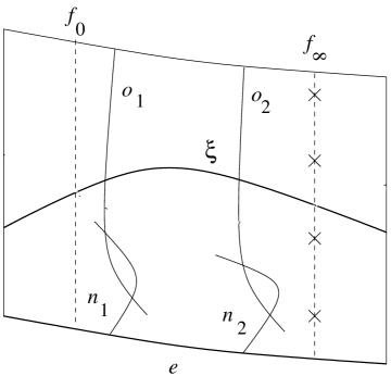
Figure 1: A special rational elliptic surface $B$. It has 8 $I_{1}$ singular fibers. In addition, there are 2 $I_{2}$ fibers $f_{1}=n_{1}\cup o_{1}$ and $f_{2}=n_{2}\cup o_{2}$. Under the involution $\tau_{B}=t_{\xi}\circ\alpha_{B}$, there are 4 fixed points, which we have marked, on the fiber $f_{\infty}$.

Figure 2: The Calabi-Yau threefold $\tilde{X}$ is constructed as the fiber product over $\mathbb{P}^{1}$ of two non-generic $dP_{9}$ surfaces $B$ and $B^{\prime}$. We have matched the fibers $f_{0}$ and $f_{\infty}$ of $B$ with the fibers $f^{\prime}_{\infty}$ and $f^{\prime}_{0}$ of $B^{\prime}$ respectively. The image points in $\mathbb{P}^{1}$ of these fibers, namely $0$ and $\infty$ for $B$ and $0^{\prime}$ and $\infty^{\prime}$ for $B^{\prime}$, are identified as $0=\infty^{\prime}$ and $\infty=0^{\prime}$.

3.3 Building $\tilde{X},\tau$ and $A$

Choose two special rational elliptic surfaces $\beta:B\rightarrow\mathbb{P}^{1}$ and $\beta^{\prime}:B^{\prime}\rightarrow\mathbb{P}^{1}$ in $\tilde{X}$ so that the discriminant loci of $\beta$ and $\beta^{\prime}$ in $\mathbb{P}^{1}$ are disjoint, $\alpha_{B}$ and $\alpha_{B^{\prime}}$ induce the same involution on $\mathbb{P}^{1}$, and the fixed loci of $\tau_{B}$ and $\tau_{B^{\prime}}$ sit over different points 0 and $\infty$ in $\mathbb{P}^{1}$. The fiber product $\tilde{X}=B\times_{\mathbb{P}^{1}}B^{\prime}$ is a smooth Calabi-Yau threefold which is elliptic and has a freely acting involution $\tau:=\tau_{B}\times_{\mathbb{P}^{1}}\tau_{B^{\prime}}$ and another (non-free) involution $\alpha_{X}:=\alpha_{B}\times_{\mathbb{P}^{1}}\alpha_{B^{\prime}}$. For concreteness we fix the elliptic fibration of $\tilde{X}$ to be the projection $\pi:\tilde{X}\rightarrow B^{\prime}$ to $B^{\prime}$. The structure of $\tilde{X}$ is shown in Figure 2.

The stability of the bundle $\tilde{V}$ which we describe below is with respect to a particular choice of Kähler class $A$. If $A_{0}$ is any Kähler class on $\tilde{X}$, $h^{\prime}$ a Kähler class on $B^{\prime}$, and $n\gg 0$, the class of $A=A_{0}+n\pi^{*}h^{\prime}$ will be Kähler on $\tilde{X}$. The specific value that was found in [49] to satisfy all the requirements was given by $h^{\prime}=193f^{\prime}+144e_{1}^{\prime}+168(e_{9}^{\prime}+e_{4}^{\prime}-e_{5}^{\prime})$.

3.4 The Construction of $V$

The construction of the $SU(5)$ bundle $V$ on $X:=\tilde{X}/F$ is equivalent to the construction of an $SU(5)$ bundle $\tilde{V}$ on $\tilde{X}$ together with an action of the involution $\tau$ on $\tilde{V}$. The construction of $\tilde{V}$ in [49] employs a combination of two techniques: extensions and the spectral construction.

The rank 5 bundle $\tilde{V}$ is constructed as an extension

$$0\rightarrow V_{2}\rightarrow\tilde{V}\rightarrow V_{3}\rightarrow 0$$ (42)

involving two simpler bundles $V_{2}$, $V_{3}$, of ranks 2 and 3 respectively. Given the $V_{i}$, we can immediately construct their direct sum $\tilde{V}_{0}=V_{2}\oplus V_{3}$, which is the trivial extension. In terms of an open cover $\{U_{\alpha}\}$ and $i\times i$ transition matrices $\{g_{i\alpha\beta}\}$ for each $V_{i}$, the transition matrices for $\tilde{V}_{0}$ are

$$g_{0\alpha\beta}=\left(\matrix{g_{2\alpha\beta}&0\cr 0&g_{3\alpha\beta}}\right)\ .$$ (43)

A general extension $\tilde{V}$ is a rank 5 bundle containing $V_{2}$ as a subbundle with quotient $V_{3}$, but $V_{3}$ cannot be realized as a subbundle of $\tilde{V}$ unless $\tilde{V}$ is the trivial extension $\tilde{V}_{0}$. The transition matrices for such an extension must be of the form:

$$g_{\alpha\beta}=\left(\matrix{g_{2\alpha\beta}&h_{\alpha\beta}\cr 0&g_{3\alpha\beta}}\right)\ .$$ (44)

In order for these $g_{\alpha\beta}$ to define a vector bundle, the upper right corner $h_{\alpha\beta}$ must satisfy a cocycle condition. Working this out shows that the set of isomorphism classes of extensions is described by the sheaf cohomology group:

$${\rm Ext}^{1}_{\tilde{X}}(V_{3},V_{2}):=H^{1}(\tilde{X},V_{3}^{*}\otimes V_{2})\ .$$ (45)

The direct sum $\tilde{V}_{0}=V_{2}\oplus V_{3}$ corresponds to the 0 element of this extension group. Our standard model bundle $\tilde{V}$ turns out to correspond to a non-trivial extension $[\tilde{V}]\in{\rm Ext}_{\tilde{X}}^{1}(V_{3},V_{2})$. In order for $\tilde{V}$ to be $\tau$-invariant, we require first that $V_{2}$ and $V_{3}$ be $\tau$-invariant, so we can choose an action of $\tau$ on $V_{2}$ and $V_{3}$. This induces an action of $\tau$ on ${\rm Ext}_{\tilde{X}}^{1}(V_{3},V_{2})$. In order for $\tilde{V}$ to be $\tau$-invariant, we require that the extension class $[\tilde{V}]$ be $\tau$-invariant.

3.5 The Construction of the $V_{i}$

The construction of the bundles $V_{i}$, $i=2,3$, involves the spectral construction or Fourier-Mukai transform [2, 3, 4]. The Fourier-Mukai transform is a self-equivalence of the derived category $D^{b}(\tilde{X})$ of coherent sheaves on $\tilde{X}$

$$FM: D^{b}(\tilde{X})\rightarrow D^{b}(\tilde{X})$$ (46)

$${\mathcal{F}}\rightarrow Rp_{1*}(p_{2}^{*}{\mathcal{F}}\stackrel{{\scriptstyle L}}{{\otimes}}{\mathcal{P}})\ .$$

Here, $p_{1}$, $p_{2}$ are the projections of the fiber product $\tilde{X}\times_{B^{\prime}}\tilde{X}$ to the two $\tilde{X}$ factors, $Rp_{1*}$ is the right derived functor of $p_{1*}$, ${\mathcal{P}}$ is the Poincaré sheaf on $\tilde{X}\times_{B^{\prime}}\tilde{X}$, and $\stackrel{{\scriptstyle L}}{{\otimes}}$ is the left derived functor of $\otimes$. If $V_{i}$ is a rank $i$ vector bundle on $\tilde{X}$ which is semistable and of degree 0 on each elliptic fiber $f$ of $\pi:\tilde{X}\rightarrow B^{\prime}$, then $FM^{-1}(V_{i})$ is a rank 1 sheaf $N_{\Sigma_{i}}$ supported on a divisor $\Sigma_{i}\subset\tilde{X}$ which is finite of degree $i$ over the base $B^{\prime}$. In other words, $\Sigma_{i}$ intersects each elliptic fiber $f$ in $i$ points. In case $\Sigma_{i}$ is smooth, $N_{\Sigma_{i}}$ is actually a line bundle on $\Sigma_{i}$. The spectral construction starts with $(\Sigma_{i},N_{\Sigma_{i}})$ and recovers the bundle $V_{i}$ as the Fourier-Mukai transform. When $\Sigma_{i}$ is irreducible, the resulting bundle $V_{i}$ is automatically stable.

In our case we do not need the full spectral construction on the threefold $\tilde{X}$. The map $\beta:B\rightarrow\mathbb{P}^{1}$ is an elliptic fibration, so there is a Fourier-Mukai transform $FM_{B}$ on $D^{b}(B)$. We will describe below certain curves $C_{i}\subset B$ and line bundles $N_{i}\in Pic(C_{i})$ for $i=2,3$. These determine two bundles $W_{i}:=FM_{B}(C_{i},N_{i})$ with $\mbox{rk}(W_{i})=i$. Our desired bundles $V_{i}$ are then recovered as

$$V_{i}=\pi^{\prime*}W_{i}\otimes\pi^{*}L_{i}$$ (47)

for appropriate line bundles $L_{i}\in Pic(B^{\prime})$. The spectral data on $B$ and on $\tilde{X}$ are related by

$$\Sigma_{i}=(\pi^{\prime})^{-1}C_{i}=C_{i}\times_{\mathbb{P}^{1}}B^{\prime},\qquad N_{\Sigma_{i}}=(\pi^{\prime})^{*}N_{i}\otimes\pi^{*}L_{i}\ .$$ (48)

This is summarized in Figure 3.

Figure 3: The structure of the vector bundles $V_{i}$, $i=2,3$.

The specific values we take for the $C_{i}$, $N_{i}$ and $L_{i}$ are as follows. Choose curves $\overline{C}_{2},C_{3}\subset B$, so that

$$\begin{array}[]{lcl}\bullet&&\overline{C}_{2}\in|{\mathcal{O}}_{B}(2e_{9}+2f)|,\quad C_{3}\in|{\mathcal{O}}_{B}(3e_{9}+6f)|,\\ \bullet&&\mbox{$\overline{C}_{2}$ and $C_{3}$ are $\alpha_{B}$-invariant,}\\ \bullet&&\mbox{$\overline{C}_{2}$ and $C_{3}$ are smooth and irreducible.}\end{array}$$

Set $C_{2}=\overline{C}_{2}+f_{\infty}$ where $f_{\infty}$ is the smooth fiber of $\beta$ containing the four fixed points of $\tau_{B}$. We choose the line bundles $N_{2}\in Pic^{3,1}(C_{2})$, $N_{3}\in Pic^{16}(C_{3})$ to transform correctly under the involution $\alpha_{B}|_{C_{i}}$:

$$N_{i}\simeq(\alpha_{B}|_{C_{i}})^{*}N_{i}\otimes{\mathcal{O}}_{C_{i}}(e_{1}-e_{9}+f),\qquad i=2,3\ .$$ (49)

Here $Pic^{3,1}(C_{2})$ denotes line bundles of degree 3 on $\overline{C}_{2}$ and degree 1 on $f_{\infty}$ [49]. (It is shown in [49] that such $N_{i}$ do exist.) A useful quantity associated with the bundle $W_{2}$ is the degree $-1$ line bundle $G\in Pic^{-1}(f_{\infty})$ on the elliptic curve $f_{\infty}$, defined as

$$G=N_{2}|_{f_{\infty}}(-D),$$ (50)

where $D$ is the divisor $D=\overline{C}_{2}\cap f_{\infty}$. This fits into an exact sequence

$$0\rightarrow W_{2}\rightarrow\overline{W}_{2}\rightarrow i_{f_{\infty}*}(G^{*})\rightarrow 0\ ,$$ (51)

where $\overline{W}_{2}$ is the rank 2 vector bundle associated with the spectral cover $\overline{C}_{2}$ and spectral line bundle $\overline{N}_{2}=N_{2}\otimes{\mathcal{O}}_{\overline{C}_{2}}$. The Chern characters can be read from Lemma 5.1 of [49]:

$$\begin{array}[]{cc}\mbox{ch}(W_{2})=2-f-3{\rm pt},&\mbox{ch}(\overline{W}_{2})=2-2{\rm pt},\\ \mbox{ch}(W_{3})=3+f-6{\rm pt},&\mbox{ch}(G^{*})=f+{\rm pt}.\end{array}$$

Finally, the line bundles $L_{i}$ on $B^{\prime}$ are given by

$$L_{2} = {\mathcal{O}}_{B^{\prime}}(3r^{\prime})$$

$$L_{3} = {\mathcal{O}}_{B^{\prime}}(-2r^{\prime})$$ (52)

where

$$r^{\prime}=e_{1}^{\prime}+e_{4}^{\prime}-e_{5}^{\prime}+e_{9}^{\prime}+f^{\prime}=3\ell^{\prime}-2e_{4}^{\prime}-(e_{2}^{\prime}+e_{3}^{\prime}+e_{6}^{\prime}+e_{7}^{\prime}+e_{8}^{\prime}).$$ (53)

Formula (3.5) holds with the specific choices $N_{2}\in Pic^{3,1}(C_{2})$, $N_{3}\in Pic^{16}(C_{3})$ which we made above, and only with those choices. This is why we specify the general solution in [49] to these values.

This completes the specification of the bundles $V_{i}$ for $i=2,3$. It was seen in [49] that $\tau$-invariant extensions $[\tilde{V}]\in{\rm Ext}_{\tilde{X}}^{1}(V_{3},V_{2})_{(+)}$ exist, and that the bundle $\tilde{V}$ corresponding to a general such $[\tilde{V}]$ has structure group $G=SU(5)$, is stable, is $\tau$-invariant, and satisfies the requirements $(\mathbb{Z}_{2},S,I,C1,C2,C3)$ in (3).

3.6 Comments

The reason we did not build $\tilde{V}$ directly by a spectral construction applied to the surface $\Sigma=\Sigma_{2}\cup\Sigma_{3}$ in $\tilde{X}$ (or to the curve $C=C_{2}\cup C_{3}$ in $B$) is that on singular spectral covers (such as $\Sigma$, $C$), the rank 1 sheaf ($\overline{N}$ or $N$) can fail to be a line bundle, leading to technical complications. A closely related problem is that it is harder to check the stability of $\tilde{V}$ when the spectral cover is reducible.

Another subtlety is that our $C_{2}$ is not finite over $\mathbb{P}^{1}$. It intersects the generic elliptic fiber in 2 points, but it contains the entire fiber $f_{\infty}$. We chose $N_{2}$ carefully so that our $W_{2}$ is still the Fourier-Mukai transform of $(C_{2},N_{2})$. But in practice it is often easier to work with $\overline{C}_{2}$, $\overline{N}_{2}$ and $\overline{W}_{2}$, and to relate $W_{2}$ and $\overline{W}_{2}$ via (51).

The construction in [49] involves additional degrees of freedom in the form of Hecke transforms applied to the $\tilde{V}$. Later checks, motivated by questions of Mike Douglas, suggest that most or all of these extra degrees of freedom may be illusory. At any rate, we do not use them in the present work.

4 Cohomologies of $U_{i}(\tilde{V})$

In order to compute the relevant cohomologies on a rational elliptic surface such as $B^{\prime}$, we need some basic facts about the line bundle ${\mathcal{O}}_{B^{\prime}}(r^{\prime})$ of (53). We claim that the direct image is:

$$\beta^{\prime}_{*}{\mathcal{O}}_{B^{\prime}}(r^{\prime})\simeq{\mathcal{O}}_{\mathbb{P}^{1}}\oplus{\mathcal{O}}_{\mathbb{P}^{1}},$$ (54)

or equivalently that

$$\beta^{\prime}_{*}{\mathcal{O}}_{B^{\prime}}(r^{\prime}-f^{\prime})\simeq{\mathcal{O}}_{\mathbb{P}^{1}}(-1)\oplus{\mathcal{O}}_{\mathbb{P}^{1}}(-1).$$ (55)

Indeed, the left hand side of (55) is a rank 2 bundle on $\mathbb{P}^{1}$, since $(r^{\prime}-f^{\prime})\cdot f^{\prime}=2$, so it must be of the form ${\mathcal{O}}_{\mathbb{P}^{1}}(a)\oplus{\mathcal{O}}_{\mathbb{P}^{1}}(b)$ for some integers $a$, $b$. Now $r^{\prime}-f^{\prime}=e_{1}^{\prime}+e_{9}^{\prime}+e_{4}^{\prime}-e_{5}^{\prime}$ cannot be effective (any effective representative has negative intersection with $e_{1}^{\prime}$, $e_{4}^{\prime}$, $e_{9}^{\prime}$, so must contain all of them), and therefore our integers $a$, $b$ must be negative. To conclude that $a=b=-1$ as claimed in (55), it suffices to note that $a+b$ is the degree of $\beta^{\prime}_{*}{\mathcal{O}}_{B^{\prime}}(r^{\prime}-f^{\prime})$, which by Groethendieck-Riemann-Roch (GRR) equals $-2$.

Instead of GRR, we can obtain the same result using a bit of geometry. We saw in (53) that $r^{\prime}=3\ell^{\prime}-(e_{2}^{\prime}+e_{3}^{\prime}+e_{6}^{\prime}+e_{7}^{\prime}+e_{8}^{\prime})-2e_{4}^{\prime}$, so we can identify sections of ${\mathcal{O}}_{B^{\prime}}(r^{\prime})$ with cubic polynomials on $\mathbb{P}^{2}$ vanishing at $A_{i}$ for $i=2,3,6,7,8$, and vanishing to second order at $A_{4}$. The space $H^{0}({\mathcal{O}}_{\mathbb{P}^{2}}(3\ell))$ of cubics is 10 dimensional, the vanishing at each of the five $A_{i}$ imposes one linear condition, and vanishing to second order at $A_{4}$ imposes 3 more conditions, for a total of 8 conditions. Therefore $2=10-8\leq h^{0}({\mathcal{O}}_{B^{\prime}}(r^{\prime}))=h^{0}(\mathbb{P}^{1},\beta^{\prime}_{*}{\mathcal{O}}_{B^{\prime}}(r^{\prime}))=h^{0}({\mathcal{O}}_{\mathbb{P}^{1}}(a+1))+h^{0}({\mathcal{O}}_{\mathbb{P}^{1}}(b+1))$. Recalling that $a$, $b$ are negative, this is possible only for $a=b=-1$; so we have found another argument for (54), (55).

It follows from (54) that $H^{0}({\mathcal{O}}_{B^{\prime}}(r^{\prime}))$ is 2 dimensional. We let $x_{0}$ and $x_{1}$ be a basis. We claim that the quotient $x_{1}/x_{0}$ is everywhere defined, so it gives a map

$$\chi:B^{\prime}\rightarrow\mathbb{P}^{1}_{x},$$ (56)

and the $x_{i}$ can be interpreted as homogeneous coordinates on the target $\mathbb{P}^{1}_{x}$. Checking that $\chi$ is everywhere defined is equivalent to verifying that $x_{0}$ and $x_{1}$ cannot vanish at the same point. Since $r^{\prime 2}=0$, two divisors in the linear system $|r^{\prime}|$ cannot intersect each other unless they have a common component. So to conclude, it suffices to check that some (and hence almost all) of these divisors are irreducible. This follows immediately from the geometric model: in fact, the fibers of $\chi$, identified as the pencil of cubics vanishing at the five $e_{i}^{\prime}$ and doubly at $e_{4}^{\prime}$, include precisely 8 reducible curves, namely:

$$\begin{array}[]{lll}K_{i}^{1}\cup K_{i}^{2},&K_{i}^{1}=\ell^{\prime}-e_{5}^{\prime}-e_{i}^{\prime},&K_{i}^{2}=2\ell^{\prime}-(e_{2}^{\prime}+e_{3}^{\prime}+e_{6}^{\prime}+e_{7}^{\prime}+e_{8}^{\prime})-e_{5}^{\prime}+e_{i}^{\prime},\quad i=2,3,6,7,8\\ K_{j}^{0}\cup K_{j}^{3},&K_{j}^{0}=e_{j}^{\prime},&K_{j}^{3}=3\ell^{\prime}-(e_{2}^{\prime}+e_{3}^{\prime}+e_{6}^{\prime}+e_{7}^{\prime}+e_{8}^{\prime})-2e_{5}^{\prime}-e_{j}^{\prime},\quad j=1,4,9.\end{array}$$ (57)

The first five curves occur as reducible cubics in $\mathbb{P}^{2}$, consisting of the line joining $A_{5}$ to $A_{i}$ and the conic through $A_{5}$ and the remaining 4 points. The last three consist of cubics which happen to pass through one of the $A_{j}$, so their inverse image in $B^{\prime}$ contains the corresponding $e_{j}^{\prime}$. All other cubics in our system are singular (at $A_{5}$) but irreducible. We conclude that $\chi$ is indeed everywhere defined, its generic fiber is a $\mathbb{P}^{1}$, and precisely the 8 fibers listed in (57) split into a pair of $\mathbb{P}^{1}$’s meeting at one point.

Clearly, the target space $\mathbb{P}^{1}_{x}$ of the map $\chi$ defined by the line bundle ${\mathcal{O}}_{B^{\prime}}(r^{\prime})$ has nothing to do with the target space $\mathbb{P}^{1}_{t}$ of the map $\beta^{\prime}$ defined by the line bundle ${\mathcal{O}}_{B^{\prime}}(f^{\prime})$. In fact, we can put these two maps together, to get a map

$$\Delta=(\beta^{\prime},\chi):B^{\prime}\rightarrow{\sf Q}:=\mathbb{P}^{1}_{t}\times\mathbb{P}^{1}_{x}$$ (58)

given by the two pairs of homogeneous coordinates $(t_{0},t_{1})$, $(x_{0},x_{1})$.

The product surface ${\sf Q}$ could be identified with a smooth quardric in $\mathbb{P}^{3}$ via the embedding $(t_{0}x_{0},t_{1}x_{0},t_{0}x_{1},t_{1}x_{1})$, but we will not use this. The product map $\Delta$ is onto ${\sf Q}$, and is of degree $f^{\prime}\cdot r^{\prime}=2$; in other words, we have realized the rational elliptic surface $B^{\prime}$ as a double cover of the quadric surface ${\sf Q}$. The fibers of $\beta^{\prime}$ are of course the elliptic curves $f^{\prime}$ which now appear as double covers of $\mathbb{P}^{1}_{x}$ branched at 4 points. The general fiber of $\chi$, on the other hand, is isomorphic to a $\mathbb{P}^{1}$, as is seen by adjunction. It appears as a double cover of $\mathbb{P}^{1}_{t}$ branched at 2 points. The branch locus $Br_{\Delta}$ of $\Delta$ is therefore a divisor of bidegree $(4,2)$ in Q .

Line bundles on Q are of the form ${\mathcal{O}}_{{\sf Q}}(k,l):=pr_{t}^{*}{\mathcal{O}}_{\mathbb{P}^{1}_{t}}(l)\otimes pr_{x}^{*}{\mathcal{O}}_{\mathbb{P}^{1}_{x}}(k)$, with integers $k$, $l$, where $pr_{t}$, $pr_{x}$ are the projections to $\mathbb{P}^{1}_{t}$, $\mathbb{P}^{1}_{x}$ respectively: $\beta^{\prime}=pr_{t}\circ\Delta$, $\chi=pr_{x}\circ\Delta$. Let us introduce the abbreviation

$${\mathcal{O}}_{B^{\prime}}(k,l):=\Delta^{*}{\mathcal{O}}_{{\sf Q}}(k,l)={\mathcal{O}}_{B^{\prime}}(kr^{\prime}+lf^{\prime})$$ (59)

for the corresponding line bundles on $B^{\prime}$. So for example ${\mathcal{O}}_{B^{\prime}}(0,1)$ is the anticanonical bundle $K_{B^{\prime}}^{-1}\simeq{\mathcal{O}}_{B^{\prime}}(f^{\prime})$, ${\mathcal{O}}_{B^{\prime}}(1,0)$ is ${\mathcal{O}}_{B^{\prime}}(r^{\prime})$, ${\mathcal{O}}_{B^{\prime}}(3,0)$ is our $L_{2}$, and ${\mathcal{O}}_{B^{\prime}}(-2,0)$ is $L_{3}$.

On $B^{\prime}$ there is a unique involution $\iota$ which exchanges the two sheets of $B^{\prime}$ over Q . Its fixed locus is the ramification divisor $Ram_{\Delta}\subset B^{\prime}$. The image $\Delta(Ram_{\Delta})$ is of course $Br_{\Delta}$. Since

$$\Delta^{*}{\mathcal{O}}_{{\sf Q}}(Br_{\Delta})={\mathcal{O}}_{B^{\prime}}(2Ram_{\Delta})$$ (60)

and the Picard group of $B^{\prime}$ has no torsion, we find that:

$${\mathcal{O}}_{B^{\prime}}(Ram_{\Delta})\simeq\Delta^{*}{\mathcal{O}}_{{\sf Q}}\left(\frac{1}{2}Br_{\Delta}\right)=\Delta^{*}{\mathcal{O}}_{{\sf Q}}(2,1)={\mathcal{O}}_{B^{\prime}}(2,1).$$ (61)

For any double cover such as $\Delta$, sections of ${\mathcal{O}}_{B^{\prime}}$ can be decomposed into $\iota$-invariants and anti-invariants. This can be written formally as a decomposition of the direct image:

$$\Delta_{*}{\mathcal{O}}_{B^{\prime}}\simeq 1\cdot{\mathcal{O}}_{{\sf Q}}\oplus y\cdot{\mathcal{O}}_{{\sf Q}}\left(-\frac{1}{2}Br_{\Delta}\right),$$ (62)

where $y\in H^{0}({\mathcal{O}}_{B^{\prime}}(Ram_{\Delta}))$ is the $\iota$-anti-invariant section characterized up to scalars by its vanishing precisely on $Ram_{\Delta}$. (This is another special case of GRR). In our case, (61) shows that

$$y\in H^{0}({\mathcal{O}}_{B^{\prime}}(2,1)),\quad\iota y=-y$$ (63)

and

$$\Delta_{*}{\mathcal{O}}_{B^{\prime}}={\mathcal{O}}_{{\sf Q}}\oplus y{\mathcal{O}}_{{\sf Q}}(-2,-1).$$ (64)

This can be tensored with the pullback of ${\mathcal{O}}_{{\sf Q}}(k,l)$, giving the decomposition

$$\Delta_{*}{\mathcal{O}}_{B^{\prime}}(k,l)={\mathcal{O}}_{{\sf Q}}(k,l)\oplus y{\mathcal{O}}_{{\sf Q}}(k-2,l-1)$$ (65)

which will be the foundation for our cohomological calculations.

Let $S_{x}^{k}:=H^{0}({\mathcal{O}}_{\mathbb{P}^{1}_{x}}(k))$ denote the $(k+1)$-dimensional vector space of homogeneous polynomials of degree $k\geq 0$ in $x_{0},x_{1}$, with basis consisting of the monomials $x_{0}^{k},x_{0}^{k-1}x_{1},\ldots,x_{1}^{k}$. We set $S_{x}^{k}=0$ for $k<0$, and let $(S_{x}^{k})^{*}$ denote the dual vector space. The cohomology of $\mathbb{P}^{1}_{x}$ is given by:

$$H^{0}({\mathcal{O}}_{\mathbb{P}^{1}_{x}}(k))=S_{x}^{k},\quad H^{1}({\mathcal{O}}_{\mathbb{P}^{1}_{x}}(k))\simeq(S_{x}^{-2-k})^{*},$$ (66)

where the second formula involves Serre duality and therefore depends on choosing, once and for all, an isomorphism of $K_{\mathbb{P}^{1}_{x}}$ with ${\mathcal{O}}_{\mathbb{P}^{1}_{x}}(-2)$. This formula can be applied to the product surface ${\sf Q}=\mathbb{P}^{1}_{t}\times\mathbb{P}^{1}_{x}$, yielding a formula for the direct images (for a general definition of direct image sheaves we refer the reader to the Appendix)

$$R^{i}pr_{t*}{\mathcal{O}}_{{\sf Q}}(k,l)=H^{i}({\mathcal{O}}_{\mathbb{P}^{1}_{x}}(k))\otimes{\mathcal{O}}_{\mathbb{P}^{1}_{t}}(l)\simeq\left\{\begin{array}[]{ll}S_{x}^{k}\otimes{\mathcal{O}}_{\mathbb{P}^{1}_{t}}(l),&i=0\\ (S_{x}^{-2-k})^{*}\otimes{\mathcal{O}}_{\mathbb{P}^{1}_{t}}(l),&i=1\end{array}\right.\ ,$$ (67)

and therefore for the cohomology:

$$H^{n}({\mathcal{O}}_{{\sf Q}}(k,l)) = \bigoplus_{i+j=n}H^{i}({\mathcal{O}}_{\mathbb{P}^{1}_{x}}(k))\otimes H^{j}({\mathcal{O}}_{\mathbb{P}^{1}_{t}}(l))$$ (71)

$$\simeq \left\{\begin{array}[]{ll}S_{x}^{k}\otimes S_{t}^{l},&n=0\\ (S_{x}^{-2-k})^{*}\otimes S_{t}^{l}\oplus S_{x}^{k}\otimes(S_{t}^{-2-l})^{*},&n=1\\ (S_{x}^{-2-k})^{*}\otimes(S_{t}^{-2-l})^{*}&n=2.\end{array}\right.$$

The power of formula (65) is that it allows us to write down analogous formulas for the much more complicated surface $B^{\prime}$:

$$\begin{array}[]{ccccc}\beta^{\prime}_{*}{\mathcal{O}}_{B^{\prime}}(k,l)&=&S_{x}^{k}\otimes{\mathcal{O}}_{\mathbb{P}^{1}_{t}}(l)&\oplus&yS_{x}^{k-2}\otimes{\mathcal{O}}_{\mathbb{P}^{1}_{t}}(l-1)\\ R^{1}\beta^{\prime}_{*}{\mathcal{O}}_{B^{\prime}}(k,l)&\simeq&(S_{x}^{-2-k})^{*}\otimes{\mathcal{O}}_{\mathbb{P}^{1}_{t}}(l)&\oplus&y(S_{x}^{-k})^{*}\otimes{\mathcal{O}}_{\mathbb{P}^{1}_{t}}(l-1).\end{array}$$

Note that for $k>0$ only the $\beta^{\prime}_{*}$ term is non-zero, while for $k<0$ only the $R^{1}\beta^{\prime}_{*}$ term is non-zero. The cohomology on $B^{\prime}$ can be obtained from (4), or directly from (65):

$$H^{n}({\mathcal{O}}_{B^{\prime}}(k,l))=H^{n}({\mathcal{O}}_{{\sf Q}}(k,l))\oplus yH^{n}({\mathcal{O}}_{{\sf Q}}(k-2,l-1)),$$ (72)

where the individual terms are given in (71).

Explicitly, this formula gives bases for the various cohomology groups on $B^{\prime}$ consisting of monomials in $t_{0},t_{1},x_{0},x_{1},y$. For example:

$$\begin{array}[]{ll}H^{0}({\mathcal{O}}_{B^{\prime}}(0,1)):&t_{0},t_{1}\\ H^{0}({\mathcal{O}}_{B^{\prime}}(1,0)):&x_{0},x_{1}\\ H^{0}({\mathcal{O}}_{B^{\prime}}(3,0)):&x_{0}^{3},x_{0}^{2}x_{1},x_{0}x_{1}^{2},x_{1}^{3}\\ H^{0}({\mathcal{O}}_{B^{\prime}}(2,1)):&t_{0}x_{0}^{2},t_{0}x_{0}x_{1},t_{0}x_{1}^{2},t_{1}x_{0}^{2},t_{1}x_{0}x_{1},t_{1}x_{1}^{2},y.\end{array}$$ (73)

Now, we are ready to calculate the cohomology groups which we need on $\tilde{X}$.

$\bullet$ $V_{2}$

We have

$$\beta_{*}\overline{W}_{2}=\beta_{*}W_{2}=0$$ (74)

since these sheaves are torsion-free and vanish at a generic point. We also have $R^{1}\beta_{*}\overline{W}_{2}=0$ because it is supported on $\overline{C}_{2}\cap e_{9}$, which is empty. The long exact sequence induced from (51) therefore gives:

$$0=\beta_{*}\overline{W}_{2}\rightarrow\beta_{*}i_{f_{\infty}*}(G^{*})\rightarrow R^{1}\beta_{*}W_{2}\rightarrow R^{1}\beta_{*}\overline{W}_{2}\rightarrow 0,$$ (75)

so $R^{1}\beta_{*}W_{2}=\beta_{*}i_{f_{\infty}*}(G^{*})$. The Leray spectral sequence for $\pi:\tilde{X}\rightarrow B^{\prime}$ therefore gives:

$$H^{1}(\tilde{X},V_{2}) = H^{1}(\tilde{X},\pi^{\prime*}W_{2}\otimes\pi^{*}L_{2})=H^{0}(B^{\prime},R^{1}\pi_{*}\pi^{\prime*}W_{2}\otimes L_{2})$$ (76)

$$= H^{0}(B^{\prime},\beta^{\prime*}R^{1}\beta_{*}W_{2}\otimes L_{2})=H^{0}(f_{\infty},G^{*})\otimes H^{0}(f_{0}^{\prime},L_{2}).$$

Note that $h^{0}(f_{\infty},G^{*})=1$, $h^{0}(f_{0}^{\prime},L_{2})=6$, hence $h^{1}(\tilde{X},V_{2})=6$.

$\bullet$ $V_{3}$

We again have $\beta_{*}W_{3}=0$, so for $i=0,1$:

$$H^{i}(\tilde{X},V_{3})=H^{0}(B^{\prime},\beta^{\prime*}R^{i}\beta_{*}W_{3}\otimes L_{3})=H^{0}(\mathbb{P}^{1},R^{i}\beta_{*}W_{3}\otimes\beta_{*}^{\prime}L_{3})=0,$$ (77)

where we have used that $\beta^{\prime}_{*}L_{3}=0$, which holds since $L_{3}\cdot f^{\prime}=-4<0$.

$\bullet$ $\tilde{V}$

The long exact sequence induced from (42) gives:

$$0=H^{0}(\tilde{X},V_{3})\rightarrow H^{1}(\tilde{X},V_{2})\rightarrow H^{1}(\tilde{X},\tilde{V})\rightarrow H^{1}(\tilde{X},V_{3})=0,$$ (78)

so $H^{1}(\tilde{X},\tilde{V})=H^{1}(\tilde{X},V_{2})=H^{0}(f_{\infty},G^{*})\otimes H^{0}(f_{0}^{\prime},L_{2})$ by (76).

$\bullet$ $\wedge^{2}V_{2}$

From (3.5) we know that $\wedge^{2}W_{2}=c_{1}(W_{2})=-f$. But $\pi^{\prime*}{\mathcal{O}}_{B}(-f)\simeq\pi^{*}{\mathcal{O}}_{B^{\prime}}(-f^{\prime})$, since both pull back from the same sheaf ${\mathcal{O}}_{\mathbb{P}^{1}}(-1)$ on $\mathbb{P}^{1}$. Therefore,

$$\wedge^{2}V_{2}=\pi^{\prime*}\wedge^{2}W_{2}\otimes\pi^{*}(L_{2}^{\otimes 2})\simeq\pi^{*}{\mathcal{O}}_{B^{\prime}}(6,-1).$$ (79)

Combining this with:

$$\pi_{*}{\mathcal{O}}_{\tilde{X}}={\mathcal{O}}_{B^{\prime}},\quad R^{1}\pi_{*}{\mathcal{O}}_{\tilde{X}}={\mathcal{O}}_{B^{\prime}}(-f^{\prime})$$ (80)

gives us formulas for the direct images of $\wedge^{2}V_{2}$:

$$\pi_{*}\wedge^{2}V_{2}\simeq{\mathcal{O}}_{B^{\prime}}(6,-1),\quad R^{1}\pi_{*}\wedge^{2}V_{2}\simeq{\mathcal{O}}_{B^{\prime}}(6,-2).$$ (81)

We then push on to $\mathbb{P}^{1}$ as in (4), and since $R^{1}\beta^{\prime}_{*}=0$ for $k=6$, we find:

$$(\beta^{\prime}\circ\pi)_{*}\wedge^{2}V_{2} = \beta^{\prime}_{*}(\pi_{*}\wedge^{2}V_{2})=\beta^{\prime}_{*}{\mathcal{O}}_{B^{\prime}}(6,-1)=S_{x}^{6}\otimes{\mathcal{O}}_{\mathbb{P}^{1}_{t}}(-1)\oplus yS_{x}^{4}\otimes{\mathcal{O}}_{\mathbb{P}^{1}_{t}}(-2)$$

$$R^{1}(\beta^{\prime}\circ\pi)_{*}\wedge^{2}V_{2} = \beta^{\prime}_{*}(R^{1}\pi_{*}\wedge^{2}V_{2})=\beta^{\prime}_{*}{\mathcal{O}}_{B^{\prime}}(6,-2)=S_{x}^{6}\otimes{\mathcal{O}}_{\mathbb{P}^{1}_{t}}(-2)\oplus yS_{x}^{4}\otimes{\mathcal{O}}_{\mathbb{P}^{1}_{t}}(-3)$$

$$R^{2}(\beta^{\prime}\circ\pi)_{*}\wedge^{2}V_{2} = 0.$$ (82)

Since none of these sheaves have any global sections, we find the cohomology on $\tilde{X}$ by taking $H^{1}$ of the images on $\mathbb{P}^{1}_{t}$:

$$\begin{array}[]{ll}H^{0}(\tilde{X},\wedge^{2}V_{2})=0,&h^{0}(\tilde{X},\wedge^{2}V_{2})=0,\\ H^{1}(\tilde{X},\wedge^{2}V_{2})=yS_{x}^{4},&h^{1}(\tilde{X},\wedge^{2}V_{2})=5,\\ H^{2}(\tilde{X},\wedge^{2}V_{2})=S_{x}^{6}\oplus yS_{x}^{4}\otimes(S_{t}^{1})^{*},&h^{2}(\tilde{X},\wedge^{2}V_{2})=7+2\times 5=17,\\ H^{3}(\tilde{X},\wedge^{2}V_{2})=0,&h^{3}(\tilde{X},\wedge^{2}V_{2})=0.\end{array}$$ (83)

$\bullet$ $\wedge^{2}V_{2}^{*}$

The cohomology of $\wedge^{2}V_{2}^{*}$ can be obtained from that of $\wedge^{2}V_{2}$ by Serre duality. Equivalently, we can apply the above procedure to $\wedge^{2}V_{2}^{*}=\pi^{*}{\mathcal{O}}_{B^{\prime}}(-6,1)$, noting that for $k=-6$ all the $\beta^{\prime}_{*}$ terms in (4) vanish:

$$\pi_{*}\wedge^{2}V_{2}^{*}={\mathcal{O}}_{B^{\prime}}(-6,1),\quad R^{1}\pi_{*}\wedge^{2}V_{2}^{*}={\mathcal{O}}_{B^{\prime}}(-6,0).$$ (84)

$$(\beta^{\prime}\circ\pi)_{*}\wedge^{2}V_{2}^{*} = 0,$$

$$R^{1}(\beta^{\prime}\circ\pi)_{*}\wedge^{2}V_{2}^{*} = R^{1}\beta^{\prime}_{*}(\pi_{*}\wedge^{2}V_{2}^{*})=R^{1}\beta^{\prime}_{*}{\mathcal{O}}_{B^{\prime}}(-6,1)$$

$$= S_{x}^{4*}\otimes{\mathcal{O}}_{\mathbb{P}^{1}_{t}}(1)\oplus yS_{x}^{6*}\otimes{\mathcal{O}}_{\mathbb{P}^{1}_{t}},$$

$$R^{2}(\beta^{\prime}\circ\pi)_{*}\wedge^{2}V_{2}^{*} = R^{1}\beta^{\prime}_{*}(R^{1}\pi_{*}\wedge^{2}V_{2}^{*})=R^{1}\beta^{\prime}_{*}{\mathcal{O}}_{B^{\prime}}(-6,0)$$ (85)

$$= S_{x}^{4*}\otimes{\mathcal{O}}_{\mathbb{P}^{1}_{t}}\oplus yS_{x}^{6*}\otimes{\mathcal{O}}_{\mathbb{P}^{1}_{t}}(-1),$$

$$\begin{array}[]{llll}H^{0}(\tilde{X},\wedge^{2}V_{2}^{*})&=&0,&h^{0}(\tilde{X},\wedge^{2}V_{2}^{*})=0,\\ H^{1}(\tilde{X},\wedge^{2}V_{2}^{*})&=&H^{0}(\mathbb{P}^{1}_{t},S_{x}^{4*}\otimes{\mathcal{O}}_{\mathbb{P}^{1}_{t}}(1)\oplus yS_{x}^{6*}\otimes{\mathcal{O}}_{\mathbb{P}^{1}_{t}})&\\ &=&S_{x}^{4*}\otimes S^{1}_{t}\oplus yS_{x}^{6*},&h^{1}(\tilde{X},\wedge^{2}V_{2}^{*})=5\times 2+7=17,\\ H^{2}(\tilde{X},\wedge^{2}V_{2}^{*})&=&H^{0}(\mathbb{P}^{1}_{t},S_{x}^{4*}\otimes{\mathcal{O}}_{\mathbb{P}^{1}_{t}}\oplus yS_{x}^{6*}\otimes{\mathcal{O}}_{\mathbb{P}^{1}_{t}}(-1))&\\ &=&S_{x}^{4*},&h^{2}(\tilde{X},\wedge^{2}V_{2}^{*})=5,\\ H^{3}(\tilde{X},\wedge^{2}V_{2}^{*})&=&0,&h^{3}(\tilde{X},\wedge^{2}V_{2}^{*})=0.\end{array}$$ (86)

$\bullet$ $V_{2}\otimes V_{3}^{*}$

We recall that $C_{2}=\overline{C}_{2}\cup f_{\infty}$, and $W_{2}$ is related to $\overline{W}_{2}$ by sequence (51). If we tensor (51) by $W_{3}^{*}$ and push to $\mathbb{P}^{1}$ with $\beta_{*}$, we find

$$0\rightarrow\beta_{*}(i_{f_{\infty}*}G^{*}\otimes W_{3}^{*})\rightarrow{\mathcal{F}}\rightarrow\overline{{\mathcal{F}}}\rightarrow 0,$$ (87)

where

$${\mathcal{F}}:=R^{1}\beta_{*}(W_{2}\otimes W_{3}^{*}),\quad\overline{{\mathcal{F}}}:=R^{1}\beta_{*}(\overline{W}_{2}\otimes W_{3}^{*}),$$ (88)

and the last term in (87) is 0 because $G^{*}$ has degree $+1$ on $f_{\infty}$. All the sheaves in (87) have finite support:

• $\overline{{\mathcal{F}}}$ is supported on $\beta(\overline{C}_{2}\cap C_{3})$. If we choose things generically, $\overline{C}_{2}\cap C_{3}$ will consist of 12 points $p_{j}$ in $B^{\prime}$, the image $\beta(\overline{C}_{2}\cap C_{3})$ will consist of 12 distinct points $\hat{p}_{j}:=\beta(p_{j})\in\mathbb{P}^{1}$, $j=1,\ldots,12$, and $\overline{{\mathcal{F}}}$ will decompose as the sum of 12 rank 1 skyscraper sheaves ${\mathcal{F}}_{j}$ near each $\hat{p}_{j}$: $\overline{{\mathcal{F}}}=\bigoplus_{j=1}^{12}{\mathcal{F}}_{j}$.

• $\beta_{*}(i_{f_{\infty}*}G^{*}\otimes W_{3}^{*})$ is supported at $\infty\in\mathbb{P}_{t}^{1}$, and has rank 3 there. It can therefore be decomposed (non-canonically) as $\bigoplus_{j=13}^{15}{\mathcal{F}}_{j}$, with each ${\mathcal{F}}_{j}$ a rank 1 skyscraper sheaf supported at $\infty$. For $j=13,14,15$ we use $\hat{p}_{j}$ as another notation for the point $\infty\in\mathbb{P}_{t}^{1}$, the support of ${\mathcal{F}}_{j}$.

• The sequence (87) splits, so ${\mathcal{F}}=\bigoplus_{j=1}^{15}{\mathcal{F}}_{j}$.

We can now combine this with formula (4) applied to $L_{2}\otimes L_{3}^{*}={\mathcal{O}}_{B^{\prime}}(5,0)$, to compute $H^{1}(\tilde{X},V_{2}\otimes V_{3}^{*})$:

$$H^{1}(\tilde{X},V_{2}\otimes V_{3}^{*}) = H^{0}(\mathbb{P}^{1}_{t},R^{1}\beta_{*}(W_{2}\otimes W_{3}^{*})\otimes\beta_{*}^{\prime}(L_{2}\otimes L_{3}^{*}))$$ (89)

$$= H^{0}(\mathbb{P}^{1}_{t},{\mathcal{F}}\otimes[S_{x}^{5}\otimes{\mathcal{O}}_{\mathbb{P}^{1}_{t}}\oplus yS_{x}^{3}\otimes{\mathcal{O}}_{\mathbb{P}^{1}_{t}}(-1)])$$

$$= \bigoplus_{j=1}^{15}H^{0}(\mathbb{P}^{1}_{t},{\mathcal{F}}_{j})\otimes[S_{x}^{5}\oplus yS_{x}^{3}\otimes\{\hat{p}_{j}\mathbb{C}\}].$$

Here, we use the notation $\{\hat{p}_{j}\mathbb{C}\}\subset S_{t}^{1*}$ for the line inside the 2-dimensional plane $S_{t}^{1*}$ consisting of all points proportional to $\hat{p}_{j}\in\mathbb{P}^{1}_{t}=\mathbb{P}(S_{t}^{1*})$. This line is the fiber at $\hat{p}_{j}$ of the line bundle ${\mathcal{O}}_{\mathbb{P}^{1}_{t}}(-1)$. In particular, the dimension is

$$h^{1}(\tilde{X},V_{2}\otimes V_{3}^{*})=150=15\times[6+4].$$ (90)

$\bullet$ $V_{2}^{*}\otimes V_{3}^{*}$

From the Chern character formula (3.5) we know that $W_{2}^{*}\simeq W_{2}\otimes{\mathcal{O}}_{B^{\prime}}(f)$, and therefore

$$R^{1}\beta_{*}(W_{2}^{*}\otimes W_{3}^{*})\simeq R^{1}\beta_{*}(\beta^{*}{\mathcal{O}}_{\mathbb{P}^{1}_{t}}(1)\otimes W_{2}\otimes W_{3}^{*})={\mathcal{F}}\otimes{\mathcal{O}}_{\mathbb{P}^{1}_{t}}(1).$$ (91)

In analogy with (89) we therefore get

$$H^{2}(\tilde{X},V_{2}^{*}\otimes V_{3}^{*}) = H^{0}(\mathbb{P}^{1}_{t},R^{1}\beta_{*}(W_{2}^{*}\otimes W_{3}^{*})\otimes R^{1}\beta^{\prime}_{*}(L_{2}^{*}\otimes L_{3}^{*}))$$ (92)

$$= H^{0}(\mathbb{P}^{1}_{t},{\mathcal{F}}\otimes[yS_{x}^{1*}])$$

$$= \bigoplus_{j=1}^{15}H^{0}(\mathbb{P}^{1}_{t},{\mathcal{F}}_{j})\otimes yS_{x}^{1*},$$

and the dimension is

$$h^{2}(\tilde{X},V_{2}^{*}\otimes V_{3}^{*})=30=15\times 2.$$ (93)

$\bullet$ $\wedge^{2}\tilde{V}$

We note that the short exact sequence (42) which defines $\tilde{V}$ implies the exact sequence

$$0\rightarrow\wedge^{2}V_{2}\rightarrow\wedge^{2}\tilde{V}\rightarrow Q\rightarrow 0\ ,$$ (94)

where $Q$ is defined by the quotient of the map $\wedge^{2}V_{2}\rightarrow\wedge^{2}\tilde{V}$. However, the natural map $\wedge^{2}\tilde{V}\rightarrow\wedge^{2}V_{3}$ factors through $Q$ with the kernel $V_{2}\otimes V_{3}$. A simple consistency check for this statement is by dimension counting. Recall that $V_{2}$, $V_{3}$ and $\tilde{V}$ have rank 2, 3 and 5 respectively. Then, $Q$ has dimension $\frac{5\cdot 4}{2}-\frac{2\cdot 1}{2}=9$ from (94), $\wedge^{2}V_{3}$ has dimension $\frac{3\cdot 2}{2}=3$, so the kernel should have dimension $9-3=6$. This is indeed the dimension of $V_{2}\otimes V_{3}$, which is $2\cdot 3=6$. In summary, we have an intertwined pair of short exact sequences as follows.

$$\begin{array}[]{cccccccccc}&&&&&&0&&&\\ &&&&&&\uparrow&&&\\ &&&&&&\wedge^{2}V_{3}&&&\\ &&&&&&\uparrow&&&\\ 0&\rightarrow&\wedge^{2}V_{2}&\rightarrow&\wedge^{2}\tilde{V}&\rightarrow&Q&\rightarrow&0\ .\\ &&&&&&\uparrow&&&\\ &&&&&&V_{2}\otimes V_{3}&&&\\ &&&&&&\uparrow&&&\\ &&&&&&0&&&\end{array}$$ (95)

This then induces the following two long exact sequences in cohomology,

$$\begin{array}[]{ccccccccc}0&\rightarrow&H^{0}(\tilde{X},\wedge^{2}V_{2})&\rightarrow&H^{0}(\tilde{X},\wedge^{2}\tilde{V})&\rightarrow&H^{0}(\tilde{X},Q)&\rightarrow&\\ &\rightarrow&H^{1}(\tilde{X},\wedge^{2}V_{2})&\rightarrow&\framebox{$H^{1}(\tilde{X},\wedge^{2}\tilde{V})$}&\rightarrow&H^{1}(\tilde{X},Q)&\rightarrow&\\ &\rightarrow&H^{2}(\tilde{X},\wedge^{2}V_{2})&\rightarrow&H^{2}(\tilde{X},\wedge^{2}\tilde{V})&\rightarrow&H^{2}(\tilde{X},Q)&\rightarrow&\\ &\rightarrow&H^{3}(\tilde{X},\wedge^{2}V_{2})&\rightarrow&H^{3}(\tilde{X},\wedge^{2}\tilde{V})&\rightarrow&H^{3}(\tilde{X},Q)&\rightarrow&0\ ,\end{array}$$ (96)

and

$$\begin{array}[]{ccccccccc}0&\rightarrow&H^{0}(\tilde{X},V_{2}\otimes V_{3})&\rightarrow&H^{0}(\tilde{X},Q)&\rightarrow&H^{0}(\tilde{X},\wedge^{2}V_{3})&\rightarrow&\\ &\rightarrow&H^{1}(\tilde{X},V_{2}\otimes V_{3})&\rightarrow&H^{1}(\tilde{X},Q)&\rightarrow&H^{1}(\tilde{X},\wedge^{2}V_{3})&\rightarrow&\\ &\rightarrow&H^{2}(\tilde{X},V_{2}\otimes V_{3})&\rightarrow&H^{2}(\tilde{X},Q)&\rightarrow&H^{2}(\tilde{X},\wedge^{2}V_{3})&\rightarrow&\\ &\rightarrow&H^{3}(\tilde{X},V_{2}\otimes V_{3})&\rightarrow&H^{3}(\tilde{X},Q)&\rightarrow&H^{3}(\tilde{X},\wedge^{2}V_{3})&\rightarrow&0\ .\end{array}$$ (97)

We have boxed $H^{1}(\tilde{X},\wedge^{2}\tilde{V})$ since it is the term we wish to compute.

First consider the second sequence (97). By the same arguments as (74), we have that

$$H^{0}(\tilde{X},V_{2}\otimes V_{3})=H^{3}(\tilde{X},V_{2}\otimes V_{3})=H^{0}(\tilde{X},\wedge^{2}V_{3})=H^{3}(\tilde{X},\wedge^{2}V_{3})=0\ .$$ (98)

It then follows from (97) that

$$H^{0}(\tilde{X},Q)=H^{3}(\tilde{X},Q)=0.$$ (99)

Furthermore, using the Leray spectral sequence and the fact that $\pi_{*}\wedge^{2}V_{3}=0$ implies

$$H^{1}(\tilde{X},\wedge^{2}V_{3})\simeq H^{0}(B^{\prime},R^{1}\pi_{*}\wedge^{2}V_{3}).$$ (100)

Now,

$$R^{1}\pi_{*}\wedge^{2}V_{3}=\beta^{{}^{\prime}*}(R^{1}\beta_{*}\wedge^{2}W_{3})\otimes L_{3}^{\otimes 2}.$$ (101)

Therefore, pushing (101) down to $\mathbb{P}^{1}$, (100) becomes

$$H^{0}(B^{\prime},R^{1}\pi_{*}\wedge^{2}V_{3})=H^{0}(\mathbb{P}^{1},(R^{1}\beta_{*}\wedge^{2}W_{3})\otimes\beta^{\prime}_{*}L_{3}^{\otimes 2}).$$ (102)

Using (3.5), we see that $L_{3}^{\otimes 2}$ has negative degree along a generic fiber. Therefore, assuming that the support of $R^{1}\beta_{*}\wedge^{2}W_{3}$ is on irreducible fibers, $\beta^{\prime}_{*}L_{3}^{\otimes 2}$ vanishes and

$$H^{1}(\tilde{X},\wedge^{2}V_{3})=0\ .$$ (103)

Substituting (98) and (103) into (97) implies

$$H^{1}(\tilde{X},Q)\simeq H^{1}(\tilde{X},V_{2}\otimes V_{3})\ ,$$ (104)

and that $H^{2}(\tilde{X},Q)$ fits into the short exact sequence

$$0\rightarrow H^{2}(\tilde{X},V_{2}\otimes V_{3})\rightarrow H^{2}(\tilde{X},Q)\rightarrow H^{2}(\tilde{X},\wedge^{2}V_{3})\rightarrow 0.$$ (105)

Having established these results, let us now consider the first sequence (96). Substituting (99) into (96) gives

$$H^{0}(\tilde{X},\wedge^{2}\tilde{V})\simeq H^{0}(\tilde{X},\wedge^{2}V_{2})\ ,$$ (106)

and

$$0\rightarrow H^{1}(\tilde{X},\wedge^{2}V_{2})\rightarrow\framebox{$H^{1}(\tilde{X},\wedge^{2}\tilde{V})$}\rightarrow H^{1}(\tilde{X},Q)\rightarrow H^{2}(\tilde{X},\wedge^{2}V_{2})\rightarrow\ldots$$ (107)

Putting (104) into (107) then leads to the exact sequence

$$0\rightarrow H^{1}(\tilde{X},\wedge^{2}V_{2})\rightarrow\framebox{$H^{1}(\tilde{X},\wedge^{2}\tilde{V})$}\rightarrow H^{1}(\tilde{X},V_{2}\otimes V_{3})\stackrel{{\scriptstyle M^{T}}}{{\longrightarrow}}H^{2}(\tilde{X},\wedge^{2}V_{2})\rightarrow\ldots$$ (108)

with which we will determine the desired boxed term. In (108), we have explicitly labeled a map $M^{T}$, namely the coboundary map

$$M^{T}:H^{1}(\tilde{X},V_{2}\otimes V_{3})\rightarrow H^{2}(\tilde{X},\wedge^{2}V_{2})\ .$$ (109)

It is given by cup product with

$$[\tilde{V}]\in H^{1}(\tilde{X},V_{3}^{*}\otimes V_{2})={\rm Ext}^{1}_{\tilde{X}}(V_{3},V_{2})\ ,$$ (110)

the extension class of $\tilde{V}$, via the pairing

$$\begin{array}[]{cccccc}{\mathcal{M}}^{T}:&H^{1}(\tilde{X},V_{2}\otimes V_{3})&\times&H^{1}(\tilde{X},V_{3}^{*}\otimes V_{2})&\rightarrow&H^{2}(\tilde{X},\wedge^{2}V_{2})\\ &A&\times&B&\rightarrow&C\ .\end{array}$$ (111)

This can be dualized to

$$\begin{array}[]{cccccc}{\mathcal{M}}:&H^{1}(\tilde{X},\wedge^{2}V_{2}^{*})&\times&H^{1}(\tilde{X},V_{3}^{*}\otimes V_{2})&\rightarrow&H^{2}(\tilde{X},V_{2}^{*}\otimes V_{3}^{*})\\ &C^{*}&\times&B&\rightarrow&A^{*}\end{array}\ .$$ (112)

In formulas (86), (89) and (92) we have expressed the three cohomology groups in (112) as $H^{0}$ on $\mathbb{P}^{1}_{t}$ of appropriate sheaves. The naturality of our construction implies that the multiplication map ${\mathcal{M}}$ on cohomologies is itself induced from the natural multiplication map of the underlying sheaves on $\mathbb{P}^{1}_{t}$, namely:

$$\left(S_{x}^{4*}\otimes{\mathcal{O}}_{\mathbb{P}^{1}_{t}}(1)\oplus yS_{x}^{6*}\otimes{\mathcal{O}}_{\mathbb{P}^{1}_{t}}\right)\otimes\left({\mathcal{F}}\otimes[S_{x}^{5}\otimes{\mathcal{O}}_{\mathbb{P}^{1}_{t}}\oplus yS_{x}^{3}\otimes{\mathcal{O}}_{\mathbb{P}^{1}_{t}}(-1)]\right)\rightarrow{\mathcal{F}}\otimes yS_{x}^{1*}.$$ (113)

By taking global sections, we find that ${\mathcal{M}}$ is the product:

$${\mathcal{M}}:\left(S_{x}^{4*}\otimes S^{1}_{t}\oplus yS_{x}^{6*}\right)\otimes\left(\bigoplus_{j=1}^{15}H^{0}(\mathbb{P}^{1}_{t},{\mathcal{F}}_{j})\otimes[S_{x}^{5}\oplus yS_{x}^{3}\otimes\{\hat{p}_{j}\mathbb{C}\}]\right)\rightarrow\bigoplus_{j=1}^{15}H^{0}(\mathbb{P}^{1}_{t},{\mathcal{F}}_{j})\otimes yS_{x}^{1*}.$$ (114)

In particular, our ${\mathcal{M}}$ breaks into blocks. The three spaces involved in ${\mathcal{M}}$ have dimensions 17, 150 and 30 respectively. This breaks into 15 blocks $(j=1,\ldots,15)$, each sending a $17\times 10$ dimensional space to a 2-dimensional space. Each block breaks further into a $10\times 4\rightarrow 2$ sub-block and a $7\times 6\rightarrow 2$ sub-block, corresponding to the products

$$(S_{x}^{4*}\otimes S_{t}^{1})\otimes(S_{x}^{3}\otimes\{\hat{p}_{j}\mathbb{C}\})\rightarrow S_{x}^{1*}$$ (115)

and

$$(S_{x}^{6*})\otimes(S_{x}^{5})\rightarrow S_{x}^{1*},$$ (116)

respectively. (We have suppressed a $yH^{0}({\mathcal{F}}_{j})$ factor on each side). The transpose $M:C^{*}\rightarrow A^{*}$ of our map $M^{T}$ is obtained from (114) by evaluating at the extension class $[\tilde{V}]\in B$. We can express this $[\tilde{V}]$ in terms of its coefficients $a_{i,j}$, $i=0,\ldots,5$, $j=1,\ldots,15$ and $b_{k,j}$, $k=0,\ldots,3$, $j=1,\ldots,15$, in the $S_{x}^{5}$ and $S_{x}^{3}$ factors respectively. Now the map $S_{x}^{6*}\rightarrow S_{x}^{1*}$ given by the $a_{i,j}$ is represented by the $2\times 6$ matrix

$$M_{I,j}=\left(\begin{array}[]{ccc}a_{0,j}&\ldots~{}~{}a_{5,j}&0\\ 0&a_{0,j}~{}~{}\ldots&a_{5,j}\end{array}\right),$$ (117)

while the map $S_{x}^{4*}\otimes S_{t}^{1}\rightarrow S_{x}^{1*}$ given by the $b_{k,j}$ is represented by the $2\times 10$ matrix

$$M_{II,j}=\left(\begin{array}[]{c|c}\begin{array}[]{ccc}b_{0,j}t_{0}(\hat{p}_{j})&\ldots~{}~{}b_{3,j}t_{0}(\hat{p}_{j})&0\\ 0&b_{0,j}t_{0}(\hat{p}_{j})~{}~{}\ldots&b_{3,j}t_{0}(\hat{p}_{j})\end{array}&\begin{array}[]{ccc}b_{0,j}t_{1}(\hat{p}_{j})&\ldots~{}~{}b_{3,j}t_{1}(\hat{p}_{j})&0\\ 0&b_{0,j}t_{1}(\hat{p}_{j})~{}~{}\ldots&b_{3,j}t_{1}(\hat{p}_{j})\end{array}\end{array}\right).$$ (118)

So the full $30\times 17$ matrix $M$ is then

$$M=\left(\begin{array}[]{ccc}M_{I,1}&&M_{II,1}\\ \vdots&&\vdots\\ M_{I,15}&&M_{II,15}\end{array}\right).$$ (119)

For a generic choice of the $a_{i,j}$ and $b_{k,j}$, the rank of $M$ is 17 and $M$ is surjective. It is easy to see that this remains true also for generic $\tau$-invariant extension $[\tilde{V}]$. Plugging this, along with formulas (86) and (93), into (108), we find:

$$h^{1}(\tilde{X},\wedge^{2}\tilde{V})=5+30-17=18.$$ (120)

Using Serre duality on $\tilde{X}$ and the fact that $\mbox{ind}(\tilde{V})=\mbox{ind}(\wedge^{2}\tilde{V})=6$ [36], it is now straightforward to determine the remaining cohomology groups of $\tilde{V}$, $\tilde{V}^{*}$, $\wedge^{2}\tilde{V}$ and $\wedge^{2}\tilde{V}^{*}$.

5 The $\mathbb{Z}_{2}$ Action

In subsection 3.3 we described the involutions $\tau_{B}$, $\tau_{B^{\prime}}$, $\tau$ acting compatibly on $B$, $B^{\prime}$ and $\tilde{X}$. The action of $\tau_{B^{\prime}}$ on line bundles on $B^{\prime}$ is specified in Table 3. In particular, the line bundles ${\mathcal{O}}_{B^{\prime}}(0,1)$ and ${\mathcal{O}}_{B^{\prime}}(1,0)$ are $\tau$-invariant. It follows that there are induced involutions $\tau_{\mathbb{P}^{1}_{t}}$, $\tau_{\mathbb{P}^{1}_{x}}$ that commute with the corresponding maps $\beta^{\prime}:B^{\prime}\rightarrow\mathbb{P}^{1}_{t}$, $\chi:B^{\prime}\rightarrow\mathbb{P}^{1}_{x}$. We have already encountered the involution $\tau_{\mathbb{P}^{1}_{t}}$ in subsection 3.2, where we denoted it simply $\tau_{\mathbb{P}^{1}}$. It sends $t_{0}\mapsto t_{0},\quad t_{1}\mapsto-t_{1}$. We claim that $\tau_{\mathbb{P}^{1}_{x}}$ is also a non-trivial involution, so with an appropriate choice of the coordinates $x_{0}$, $x_{1}$ on $\mathbb{P}^{1}_{x}$ (note that we never fixed these coordinates up till now!) it acts as $x_{0}\mapsto x_{0},\quad x_{1}\mapsto-x_{1}$. For this, we must determine the action of $\tau$ on the $\mathbb{P}^{1}$ family of rational curves $r^{\prime}$. For a general, non-singular member of this family, all we learn from Table 3 is that it goes to another such. But the table also tells us the image under $\tau_{B^{\prime}}$ of each of the line bundles ${\mathcal{O}}_{B^{\prime}}(K_{i}^{d})$, as $K_{i}^{d}$ runs over the 16 components of the 8 reducible curves in the system $|r^{\prime}|$, specified in (57). Each of these has the property that $K_{i}^{d}$ is the only effective curve in its class: $h^{0}(B^{\prime},K_{i}^{d})=1$. So we can deduce from Table 3 not only the cohomology class of the image, but the actual physical image:

$$K_{2}^{d}\leftrightarrow K_{3}^{d},\quad K_{1}^{d}\leftrightarrow K_{9}^{d},\quad K_{4}^{d}\leftrightarrow K_{7}^{3-d},\quad K_{6}^{d}\leftrightarrow K_{8}^{3-d}.$$ (121)

At any rate, this clearly demonstrates that $\tau_{\mathbb{P}^{1}_{x}}$ is not the identity, as claimed.

Via the map $\Delta$, our surface $B^{\prime}$ is a double cover of ${\sf Q}=\mathbb{P}^{1}_{t}\times\mathbb{P}^{1}_{x}$. Its equation can be written explicitly as

$$y^{2}=F_{4,2}(x,t),$$ (122)

with $F_{4,2}(x,t)$ a bihomogeneous polynomial, of degree 4 in $x_{0},x_{1}$ and of degree 2 in $t_{0},t_{1}$. By (63), $y$ is a section of ${\mathcal{O}}_{B^{\prime}}(2,1)$ which vanishes on the ramification locus $Ram_{\Delta}$. Since $Ram_{\Delta}$ goes to itself under $\tau_{B^{\prime}}$, $y$ must go to a multiple of itself. Since $\tau_{B^{\prime}}$ is an involution, this multiple is $\pm 1$, so in particular $F_{4,2}$ must be invariant (rather than anti-invariant). From (63), it follows that either $\tau_{B^{\prime}}y=y$ or $\iota\tau_{B^{\prime}}y=y$. Both involutions $\tau_{B^{\prime}}$, $\iota\tau_{B^{\prime}}$ have the same properties. So by relabelling $\iota\tau_{B^{\prime}}$ as $\tau_{B^{\prime}}$ if necessary, we may as well assume that the action of $\tau_{B^{\prime}}$ is given explicitly by:

$$t_{0}\mapsto t_{0},\quad t_{1}\mapsto-t_{1},\quad x_{0}\mapsto x_{0},\quad x_{1}\mapsto-x_{1},\quad y\mapsto y.$$ (123)

In subsection 3.4 we chose compatible actions of $\tau$ on $V_{2}$, $V_{3}$ and $\tilde{V}$. It turns out that the particle spectrum on $X$ is independent of these choices and is precisely half the spectrum on $\tilde{X}$ which we computed above. We compute it as follows.

$\bullet$ $H^{1}(\tilde{X},\tilde{V})$

We have identified $H^{1}(\tilde{X},\tilde{V})$ with $H^{0}(f_{\infty},G^{*})\otimes H^{0}(f_{0}^{\prime},L_{2})$ in (76), (78). We plug $k=3$, $l=0$ into formula (65), and restrict the double cover $\Delta:B^{\prime}\rightarrow{\sf Q}$ to $\chi:f_{0}^{\prime}\rightarrow\mathbb{P}^{1}_{x}$, finding:

$$\chi_{*}{\mathcal{O}}_{f_{0}^{\prime}}(3r^{\prime})={\mathcal{O}}_{\mathbb{P}^{1}_{x}}(3)\oplus y{\mathcal{O}}_{\mathbb{P}^{1}_{x}}(1).$$ (124)

We get a natural identification of $H^{0}(f_{0}^{\prime},L_{2})=H^{0}(f_{0}^{\prime},3r^{\prime})$ with $S_{x}^{3}\oplus yS_{x}^{1}$. From (123) we see that the $\tau$ action on this 6-dimensional space has a 3-dimensional invariant subspace and 3-dimensional anti-invariant subspace. There is also a $\tau$-action on the 1-dimensional $H^{0}(f_{\infty},G^{*})$, which must be either invariant or anti-invariant. Either way, we find:

$$h^{1}(\tilde{X},\tilde{V})_{+}=3,\quad h^{1}(\tilde{X},\tilde{V})_{-}=3.$$ (125)

$\bullet$ $H^{1}(\tilde{X},\wedge^{2}\tilde{V})$

From the identification of $H^{1}(\tilde{X},\wedge^{2}V_{2})$ with $yS_{x}^{4}$ in (83), we see that

$$h^{1}(\tilde{X},\wedge^{2}V_{2})_{+}=3,\quad h^{1}(\tilde{X},\wedge^{2}V_{2})_{-}=2,$$ (126)

while the identification of $H^{2}(\tilde{X},\wedge^{2}V_{2})$ with $S_{x}^{6}\oplus yS_{x}^{4}\otimes(S_{t}^{1})^{*}$ gives

$$h^{2}(\tilde{X},\wedge^{2}V_{2})_{+}=4+5=9,\quad h^{2}(\tilde{X},\wedge^{2}V_{2})_{-}=3+5=8.$$ (127)

On the other hand, we saw in (92) that $H^{1}(\tilde{X},V_{2}\otimes V_{3})$ is dual to $\bigoplus_{j=1}^{15}H^{0}(\mathbb{P}^{1}_{t},{\mathcal{F}}_{j})\otimes(yS_{x}^{1*})$. Again, the action of $\tau$ on the 2-dimensional space $yS_{x}^{1*}$ has 1-dimensional invariants and 1-dimensional anti-invariants, so regardless of its action on the 15 1-dimensional spaces $H^{0}(\mathbb{P}^{1}_{t},{\mathcal{F}}_{j})$, we get:

$$h^{1}(\tilde{X},V_{2}\otimes V_{3})_{+}=15,\quad h^{1}(\tilde{X},V_{2}\otimes V_{3})_{-}=15.$$ (128)

Combining the last three formulae with (108) and recalling that $M^{T}$ is $\tau$-equivariant (since it is cup product with the class $[\tilde{V}]$, which was taken in subsection 3.4 to be $\tau$-invariant), we see that for those generic choices to which (120) applies we have:

$$h^{1}(\tilde{X},\wedge^{2}\tilde{V})_{+}=3+15-9=9,\quad h^{1}(\tilde{X},\wedge^{2}\tilde{V})_{-}=2+15-8=9.$$ (129)

$\bullet$ $H^{1}(\tilde{X},\tilde{V}^{*})$ and $H^{1}(\tilde{X},\wedge^{2}\tilde{V}^{*})$

The spectrum also requires the terms $H^{1}(\tilde{X},\tilde{V}^{*})$ and $H^{1}(\tilde{X},\wedge^{2}\tilde{V}^{*})$. These can be obtained from the three-family condition (C3) in (3), in conjunction with the index theorem (148), as well as Serre duality (143) presented in the Appendix. Together with the fact that $H^{0}(\tilde{X},\tilde{V})$, $H^{0}(\tilde{X},\tilde{V}^{*})=H^{3}(\tilde{X},\tilde{V})^{*}$, $H^{0}(\tilde{X},\wedge^{2}\tilde{V})$, and $H^{0}(\tilde{X},\wedge^{2}\tilde{V}^{*})=H^{3}(\tilde{X},\wedge^{2}\tilde{V})^{*}$ all vanish, we have that

$$-h^{1}(\tilde{X},U_{i}(\tilde{V}))+h^{1}(\tilde{X},U_{i}(\tilde{V^{*}}))=6,\qquad U_{i}(\tilde{V})=\tilde{V},~{}\wedge^{2}\tilde{V}\ .$$ (130)

In fact, a $\mathbb{Z}_{2}$-graded version of the index theorem implies the stronger result that

$$-h^{1}(\tilde{X},U_{i}(\tilde{V}))_{(\pm)}+h^{1}(\tilde{X},U_{i}(\tilde{V^{*}}))_{(\pm)}=3,\qquad U_{i}(\tilde{V})=\tilde{V},~{}\wedge^{2}\tilde{V}\ .$$ (131)

Alternatively, we can think of it as the index theorem applied to each of the $\tau$-invariant and anti-invariant pieces of the cohomology.

Therefore, combining (131) with (125), we have that

$$h^{1}(\tilde{X},\tilde{V}^{*})_{+}=6,\quad h^{1}(\tilde{X},\tilde{V}^{*})_{-}=6.$$ (132)

Similarly, combining (131) with (129), we have that

$$h^{1}(\tilde{X},\wedge^{2}\tilde{V})_{+}=12,\quad h^{1}(\tilde{X},\wedge^{2}\tilde{V})_{-}=12.$$ (133)

Let us summarize the conclusions of the last two sections. It is convenient to introduce the following notation. Consider, for example, the cohomology group $H^{1}(\tilde{X},\tilde{V})$. We showed in Section 4 and Section 5 that $h^{1}(\tilde{X},\tilde{V})=6$ and $h^{1}(\tilde{X},\tilde{V})_{(+)}=h^{1}(\tilde{X},\tilde{V})_{(-)}=3$ respectively. Henceforth, we will express both of these facts by writing

$$H^{1}(\tilde{X},\tilde{V})=\mathbb{C}^{3}_{(+)}\oplus\mathbb{C}^{3}_{(-)}.$$ (134)

Using this notation, we encapsulate the results of Section 4 and Section 5 in Table 4.

$$\begin{array}[]{||c|c|c|c|c|c||}\hline\cr\hline\cr U_{i}&H^{q}(\tilde{X},U_{i}(\tilde{V}))&R_{i}&h^{q}(\tilde{X},U_{i}(\tilde{V}))&A_{j}&\mathbb{C}_{(+)}^{r}\oplus\mathbb{C}_{(-)}^{s}\\ \hline\cr\hline\cr 1&H^{0}(\tilde{X},{\mathcal{O}}_{\tilde{X}})&24&1&0&\mathbb{C}_{(+)}^{1}\\ \hline\cr 10&H^{1}(\tilde{X},\wedge^{2}\tilde{V})&5&18&0&\mathbb{C}_{(+)}^{9}\\ \hline\cr&&&&1&\mathbb{C}_{(-)}^{9}\\ \hline\cr\overline{10}&H^{1}(\tilde{X},\wedge^{2}\tilde{V}^{*})&\overline{5}&24&0&\mathbb{C}_{(+)}^{12}\\ \hline\cr&&&&1&\mathbb{C}_{(-)}^{12}\\ \hline\cr 5&H^{1}(\tilde{X},\tilde{V})&\overline{10}&6&0&\mathbb{C}_{(+)}^{3}\\ \hline\cr&&&&1&\mathbb{C}_{(-)}^{3}\\ \hline\cr\overline{5}&H^{1}(\tilde{X},\tilde{V}^{*})&10&12&0&\mathbb{C}_{(+)}^{6}\\ \hline\cr&&&&1&\mathbb{C}_{(-)}^{6}\\ \hline\cr\hline\cr\end{array}$$

Table 4: The dimensions and $\mathbb{Z}_{2}$ actions on the cohomology spaces $H^{q}(\tilde{X},U_{i}(\tilde{V}))$.

6 Low Energy Spectrum

We know from the discussion in Section 2, and specifically from equation (30), that the multiplicities of the representations $B_{ij}$ of the low energy gauge group are determined by $(H^{q}(\tilde{X},U_{i}(\tilde{V}))\otimes A_{j})^{\rho^{\prime}(F)}$, the invariant part of $H^{q}(\tilde{X},U_{i}(\tilde{V}))\otimes A_{j}$ under the joint action of $\mathbb{Z}_{2}$ on $H^{q}(\tilde{X},U_{i}(\tilde{V}))$ and $A_{j}$. By combining the results in Table 2 with the $\mathbb{Z}_{2}$ action on the cohomology groups listed in Table 4, we can now compute the complete low energy spectrum of our theory. The associated multiplets descend to $X=\tilde{X}/\mathbb{Z}_{2}$ to form the $(SU(3)_{C}\times SU(2)_{L}\times U(1)_{Y})/\mathbb{Z}_{6}$ particle physics spectrum. The results are listed in Table 5. The representation $R_{i}=1$, corresponding to the moduli $H^{0}(\tilde{X},{\mathop{\rm ad}}\tilde{V})$, is not presented.

$$\begin{array}[]{||c|c|c|c||}\hline\cr\hline\cr R_{i}&A_{j}&(H^{q}(\tilde{X},U_{i}(\tilde{V}))\otimes A_{j})^{\rho^{\prime}(F)}&B_{ij}\\ \hline\cr\hline\cr 24&0&\mathbb{C}_{(+)}^{1}&(8,1)_{0}\oplus(1,3)_{0}\oplus(1,1)_{0}\\ \hline\cr 5&0&\mathbb{C}_{(+)}^{9}&(3,1)_{-2}\\ \hline\cr&1&\mathbb{C}_{(-)}^{9}&(1,2)_{3}\\ \hline\cr\overline{5}&0&\mathbb{C}_{(+)}^{12}&(\overline{3},1)_{2}\\ \hline\cr&1&\mathbb{C}_{(-)}^{12}&(1,2)_{-3}\\ \hline\cr\overline{10}&0&\mathbb{C}_{(+)}^{3}&(3,1)_{4}\oplus(1,1)_{-6}\\ \hline\cr&1&\mathbb{C}_{(-)}^{3}&(\overline{3},2)_{-1}\\ \hline\cr 10&0&\mathbb{C}_{(+)}^{6}&(\overline{3},1)_{-4}\oplus(1,1)_{6}\\ \hline\cr&1&\mathbb{C}_{(-)}^{6}&(3,2)_{1}\\ \hline\cr\hline\cr\end{array}$$

Table 5: The particle spectrum of the low-energy $(SU(3)_{C}\times SU(2)_{L}\times U(1)_{Y})/\mathbb{Z}_{6}$ theory. The $A_{j}$ correspond to characters of the $\mathbb{Z}_{2}$ representations on $R_{i}$. The $U(1)$ charges listed are $w=3Y$.

To begin with, the spectrum contains one copy of vector supermultiplets transforming under $(SU(3)_{C}\times SU(2)_{L}\times U(1)_{Y})/\mathbb{Z}_{6}$ as

$$(8,1)_{0}\oplus(1,3)_{0}\oplus(1,1)_{0}.$$ (135)

Contained in these multiplets are the gauge connections for $SU(3)_{C}$, $SU(2)_{L}$ and $U(1)_{Y}$ respectively. Furthermore, it contains three families of quarks and lepton superfields, each family transforming as

$$(3,2)_{1},\quad(\overline{3},1)_{-4},\quad(\overline{3},1)_{2}$$ (136)

and

$$(1,2)_{-3},\quad(1,1)_{6}$$ (137)

respectively. Each of these multiplets is a chiral superfield, none of which has a conjugate partner. However, there are additional chiral superfields in the spectrum. It follows from Table 5 that these occur as conjugate pairs of the $(SU(3)_{C}\times SU(2)_{L}\times U(1)_{Y})/\mathbb{Z}_{6}$ representations

$$(3,1)_{-2},\quad(1,2)_{3}$$ (138)

and

$$(3,1)_{4}\oplus(1,1)_{-6},\quad(\overline{3},2)_{-1}.$$ (139)

These multiplets represent extra matter in the spectrum, such as Higgs and other exotic fields.

Let us explain how the quark/lepton fermions and conjugate pairs arise. Consider, for example, the $B_{ij}$ representations $(\overline{3},2)_{-1}$ and $(3,2)_{1}$, corresponding to the $\overline{10}$ and 10 representations respectively. From Table 5, we see that there are 3 copies of $(\overline{3},2)_{-1}$ and 6 copies of $(3,2)_{1}$. Note that $6-3=3$ copies of $(3,2)_{1}$ are unpaired, as a consequence of the index theorem. Each unpaired $(3,2)_{1}$ multiplet contributes to a single quark/lepton generation, as in (136). This leaves 3 conjugate pairs of $(\overline{3},2)_{-1}$ and $(3,2)_{1}$ superfields. Being non-chiral pairs, these do not contribute to a quark/lepton family but, rather, are additional supermultiplets as listed in (138) and (139).

It remains to enumerate the number of additional superfields. From Table 5, we see that the spectrum has

$$n_{(3,1)_{-2}}=9,\quad n_{(1,2)_{3}}=9$$ (140)

and

$$n_{(3,1)_{4}\oplus(1,1)_{-6}}=3,\quad n_{(\overline{3},2)_{-1}}=3$$ (141)

copies of (138) and (139) respectively. The multiplicity $n_{(1,2)_{3}}$ corresponds to the number of Higgs doublet conjugate pairs in the low energy spectrum. The remaining multiplets in (138) and (139) are exotic.

We conclude that the low energy spectrum of the simple, representative model discussed in this paper includes the requisite three chiral families of quarks and leptons. Additionally, it naturally has Higgs doublet supermultiplet pairs. Unfortunately, the spectrum contains extra, exotic chiral supermultiplets which, potentially, are phenomenologically unacceptable. However, these conjugate pairs of exotic multiplets may couple to the moduli fields coming from $H^{1}(X,V\otimes V^{*})$ to form mass terms. If the moduli can acquire a sufficiently high vacuum expectation value, then the exotics multiplets will decouple at low energy and be compatible with phenomenology. These couplings will be discussed elsewhere.

Armed with the technology developed in this paper, one can now compute the spectra of standard-like models based on arbitrary stable vector bundles on a wide range of elliptically fibered Calabi-Yau threefolds. These spectra can be constrained to always contain three families of quarks and leptons. We are presently searching for such vacua with a phenomenologically acceptable number of Higgs doublets and, hopefully, no exotic matter.

Acknowledgements

We are grateful to Volker Braun and Tony Pantev for enlightening discussions. R. D. would like to acknowledge conversations with Jacques Distler. This Research was supported in part by the Department of Physics and the Maths/Physics Research Group at the University of Pennsylvania under cooperative research agreement DE-FG02-95ER40893 with the U. S. Department of Energy and an NSF Focused Research Grant DMS0139799 for “The Geometry of Superstrings.” R. D. is partially supported by an NSF grant DMS 0104354. R. R. is also supported by the Department of Physics and Astronomy of Rutgers University under grant DOE-DE-FG02-96ER40959.

Appendix A Some Useful Mathematical Facts

In this Appendix, we present some useful mathematical facts used throughout the paper [60, 61, 62]. The first is Serre duality, which implies that for a sheaf ${\mathcal{F}}$ on an $n$-fold $X$

$$H^{q}(X,{\mathcal{F}})\simeq H^{n-q}(X,{\mathcal{F}}^{*}\otimes K_{X})^{*},$$ (142)

where $K_{X}$ is the canonical bundle of $X$. For our Calabi-Yau threefold $\tilde{X}$ and sheaf $U_{i}(\tilde{V})$ on $\tilde{X}$, (142) simplifies to

$$H^{q}(\tilde{X},U_{i}(\tilde{V}))\simeq H^{3-q}(\tilde{X},U_{i}(\tilde{V})^{*})^{*},$$ (143)

where we have used the fact that $K_{\tilde{X}}$ on a Calabi-Yau manifold is trivial.

The second tool we use is the Atiyah-Singer index theorem, which implies that on our Calabi-Yau threefold $\tilde{X}$

$$\mbox{ind}(U_{i}(\tilde{V})=\sum\limits_{q=0}^{3}(-1)^{q}h^{q}(\tilde{X},U_{i}(\tilde{V}))=\int_{\tilde{X}}\mbox{ch}(U_{i}(\tilde{V}))\wedge\mbox{td}(\tilde{X})=\frac{1}{2}\int_{\tilde{X}}c_{3}(U_{i}(\tilde{V}))\ .$$ (144)

The three-generation condition means that on $X$, $\mbox{ind}(V)$ is equal to three [1], which implies that on the cover $\tilde{X}$ [49, 50],

$$\mbox{ind}(\tilde{V})=|\mathbb{Z}_{2}|\times 3=6,$$ (145)

or,

$$c_{3}(\tilde{V})=12.$$ (146)

This is the origin of the condition (C3) in (3).

In this paper, we apply the index theorem in the two cases $U_{i}(\tilde{V})=\tilde{V}$ and $\wedge^{2}\tilde{V}$. It was shown in Appendix A of [36] that for our $SU(5)$ bundle $\tilde{V}$

$$c_{3}(\wedge^{2}\tilde{V})=c_{3}(\tilde{V})=12.$$ (147)

Therefore, in these cases, (144) simplifies to

$$\sum\limits_{q=0}^{3}(-1)^{q}h^{q}(\tilde{X},U_{i}(\tilde{V}))=6,\qquad U_{i}(\tilde{V})=\tilde{V},~{}\wedge^{2}\tilde{V}\ .$$ (148)

An important tool for computing cohomology groups of vector bundles or, more generally, coherent sheaves on fibered spaces is the Leray spectral sequence. Consider the map $\pi:\tilde{X}\rightarrow B^{\prime}$ and a sheaf ${\mathcal{F}}$ on $\tilde{X}$. The Leray spectral sequence for the map $\pi$ will relate the cohomologies of ${\mathcal{F}}$ on $\tilde{X}$ to the cohomologies of the higher direct image sheaves $R^{i}\pi_{*}{\mathcal{F}}$ on $B^{\prime}$. For a general map, the sequence is rather complicated. However, in the case of $\pi$ being an elliptic fibration, it will degenerate to a simpler long exact sequence.

To begin with, consider the definition of $R^{0}\pi_{*}{\mathcal{F}}=\pi_{*}{\mathcal{F}}$. It is a sheaf on $B^{\prime}$ given by

$$\pi_{*}{\mathcal{F}}(U)={\mathcal{F}}(\pi^{-1}(U))=H^{0}(\pi^{-1}(U),{\mathcal{F}}|_{\pi^{-1}(U)})$$ (149)

for any open set $U\subset B^{\prime}$. The definition (149) generalizes to the higher image sheaves as

$$R^{i}\pi_{*}{\mathcal{F}}(U)=H^{i}(\pi^{-1}(U),{\mathcal{F}}|_{\pi^{-1}(U)})\ ,$$ (150)

for sufficiently small $U$. It follows that for the map $\pi:\tilde{X}\rightarrow B^{\prime}$

$$R^{i}\pi_{*}{\mathcal{F}}(U)=0,\qquad i>{\rm dim}\pi^{-1}(U)\ .$$ (151)

In our case, the Leray spectral sequence degenerates to the long exact sequence

$$\begin{array}[]{ccccccccc}0&\rightarrow&H^{1}(B^{\prime},\pi_{*}{\mathcal{F}})&\rightarrow&H^{1}(\tilde{X},{\mathcal{F}})&\rightarrow&H^{0}(B^{\prime},R^{1}\pi_{*}{\mathcal{F}})&\rightarrow&\\ &\rightarrow&H^{2}(B^{\prime},\pi_{*}{\mathcal{F}})&\rightarrow&H^{2}(\tilde{X},{\mathcal{F}})&\rightarrow&H^{1}(B^{\prime},R^{1}\pi_{*}{\mathcal{F}})&\rightarrow&0\ .\end{array}$$ (152)

Note that $H^{3}(B^{\prime},\pi_{*}{\mathcal{F}})=0$ since ${\rm dim}_{\mathbb{C}}B^{\prime}=2$. As promised, (152) relates the cohomology of ${\mathcal{F}}$ on $\tilde{X}$ to the cohomology of the higher image sheaves $R^{i}\pi_{*}{\mathcal{F}}$ on $B^{\prime}$. Recall that $B^{\prime}$ is itself elliptically fibered. Therefore, one can write a Leray spectral sequence for the map $\beta^{\prime}:B^{\prime}\rightarrow\mathbb{P}^{1}$ in complete analogy to (152).

Another useful formula is Groethendieck-Riemann-Roch (GRR), which states that for any map $f:X\rightarrow B$ and any sheaf ${\mathcal{S}}$ on $X$, we have

$$\mbox{td}(TB)\mbox{ch}(\sum_{i=0}^{2}(-1)^{i}R^{i}f_{*}{\mathcal{S}})=f_{*}(\mbox{ch}({\mathcal{S}})\mbox{td}(TX))\ .$$ (153)

References

• [1] M. Green, J. Schwarz and E. Witten, “Superstring theory, vol I & II,” Cambridge University Press, 1988
• [2] R. Friedman, J. Morgan and E. Witten, “Vector bundles and F theory,” Commun. Math. Phys.  187, 679 (1997). [hep-th/9701162].
• [3] R. Donagi, “Principal bundles on elliptic fibrations,” Asian J. Math., 1(2):214–223, 1997, alg-geom/9702002.
• [4] R. Friedman, J. Morgan, and E. Witten, “Vector bundles over elliptic fibrations,” J. Algebraic Geom., 8(2):279–401, 1999, alg-geom/9709029.
• [5] R. Donagi, A. Lukas, B. A. Ovrut, and D. Waldram, Non-perturbative vacua and particle physics in M-theory, JHEP 05 (1999) 018, [hep-th/9811168].
• [6] A. Lukas, B. A. Ovrut, and D. Waldram, On the four-dimensional effective action of strongly coupled heterotic string theory, Nucl. Phys. B532 (1998) 43–82, [hep-th/9710208].
• [7] A. Lukas, B. A. Ovrut, and D. Waldram, The ten-dimensional effective action of strongly coupled heterotic string theory, Nucl. Phys. B540 (1999) 230–246, [hep-th/9801087].
• [8] A. Lukas, B. A. Ovrut, and D. Waldram, Non-standard embedding and five-branes in heterotic M-theory, Phys. Rev. D59 (1999) 106005, [hep-th/9808101].
• [9] A. Lukas, B. A. Ovrut, K. S. Stelle, and D. Waldram, Heterotic M-theory in five dimensions, Nucl. Phys. B552 (1999) 246–290, [hep-th/9806051].
• [10] B. Andreas, G. Curio and A. Klemm, “Towards the standard model spectrum from elliptic Calabi-Yau,” Int. J. Mod. Phys. A 19, 1987 (2004) [arXiv:hep-th/9903052].
• [11] D. E. Diaconescu and G. Ionesei, “Spectral covers, charged matter and bundle cohomology,” JHEP 9812, 001 (1998) [arXiv:hep-th/9811129].
• [12] A. Lukas, B. A. Ovrut, K. S. Stelle, and D. Waldram, The universe as a domain wall, Phys. Rev. D59 (1999) 086001, [hep-th/9803235].
• [13] R. Donagi, A. Lukas, B. A. Ovrut, and D. Waldram, Holomorphic vector bundles and non-perturbative vacua in M- theory, JHEP 06 (1999) 034, [hep-th/9901009].
• [14] A. Lukas, B. A. Ovrut, and D. Waldram, Five-branes and supersymmetry breaking in M-theory, JHEP 04 (1999) 009, [hep-th/9901017].
• [15] Z. Lalak, S. Pokorski and S. Thomas, Beyond the Standard Embedding in M-Theory on $S^{1}/Z_{2}$, Nucl.Phys. B549 (1999) 63-97 [hep-ph/9807503].
• [16] E. I. Buchbinder, R. Donagi, and B. A. Ovrut, Vector bundle moduli superpotentials in heterotic superstrings and M-theory, JHEP 07 (2002) 066, [hep-th/0206203].
• [17] E. Buchbinder, R. Donagi, and B. A. Ovrut, Vector bundle moduli and small instanton transitions, JHEP 06 (2002) 054, [hep-th/0202084].
• [18] Y. H. He, B. A. Ovrut and R. Reinbacher, “The moduli of reducible vector bundles,” JHEP 0403, 043 (2004) [arXiv:hep-th/0306121].
• [19] E. I. Buchbinder, B. A. Ovrut and R. Reinbacher, “Instanton moduli in string theory,” arXiv:hep-th/0410200.
• [20] R. Donagi, B. A. Ovrut, and D. Waldram, Moduli spaces of fivebranes on elliptic Calabi-Yau threefolds, JHEP 11 (1999) 030, [hep-th/9904054].
• [21] B. A. Ovrut, T. Pantev, and J. Park, Small instanton transitions in heterotic M-theory, JHEP 05 (2000) 045, [hep-th/0001133].
• [22] S. Kachru and E. Silverstein, Chirality Changing Phase Transitions in 4d String Vacua, Nucl.Phys. B504 (1997) 272-284 [hep-th/9704185].
• [23] G. Curio, Chiral matter and transitions in heterotic string models, Phys.Lett. B435 (1998) 39-48 [hep-th/9803224].
• [24] M. R. Douglas and C. g. Zhou, “Chirality change in string theory,” JHEP 0406, 014 (2004) [arXiv:hep-th/0403018].
• [25] E. I. Buchbinder, R. Donagi, and B. A. Ovrut, Superpotentials for vector bundle moduli, Nucl. Phys. B653 (2003) 400–420, [hep-th/0205190].
• [26] E. Lima, B. A. Ovrut, and J. Park, Five-brane superpotentials in heterotic M-theory, Nucl. Phys. B626 (2002) 113–164, [hep-th/0102046].
• [27] E. Lima, B. A. Ovrut, J. Park, and R. Reinbacher, Non-perturbative superpotential from membrane instantons in heterotic M-theory, Nucl. Phys. B614 (2001) 117–170, [hep-th/0101049].
• [28] A. Krause, A small cosmological constant, grand unification and warped geometry, hep-th/0006226.
• [29] G. Curio and A. Krause, Four-flux and warped heterotic M-theory compactifications, Nucl. Phys. B602 (2001) 172–200, [hep-th/0012152].
• [30] G. Curio, A. Klemm, B. Kors and D. Lust, “Fluxes in heterotic and type II string compactifications,” Nucl. Phys. B 620, 237 (2002) [arXiv:hep-th/0106155].
• [31] G. Curio and A. Krause, G-fluxes and non-perturbative stabilisation of heterotic M-theory, Nucl. Phys. B643 (2002) 131–156, [hep-th/0108220].
• [32] G. Curio and A. Krause, Enlarging the parameter space of heterotic M-theory flux compactifications to phenomenological viability, Nucl. Phys. B693 (2004) 195–222, [hep-th/0308202].
• [33] G. L. Cardoso, G. Curio, G. Dall’Agata, and D. Lüst, BPS action and superpotential for heterotic string compactifications with fluxes, JHEP 10 (2003) 004, [hep-th/0306088].
• [34] G. L. Cardoso, G. Curio, G. Dall’Agata, P. M. D. Lüst, and G. Zoupanos, Non-Kähler string backgrounds and their five torsion classes, Nucl. Phys. B652 (2003) 5–34, [hep-th/0211118].
• [35] R. Donagi, Y. H. He, B. A. Ovrut and R. Reinbacher, “Moduli dependent spectra of heterotic compactifications,” arXiv:hep-th/0403291.
• [36] R. Donagi, Y. H. He, B. A. Ovrut and R. Reinbacher, “The particle spectrum of heterotic compactifications,” arXiv:hep-th/0405014.
• [37] J. Khoury, B. A. Ovrut, P. J. Steinhardt, and N. Turok, Density perturbations in the ekpyrotic scenario, Phys. Rev. D66 (2002) 046005, [hep-th/0109050].
• [38] J. Khoury, B. A. Ovrut, N. Seiberg, P. J. Steinhardt, and N. Turok, From big crunch to big bang, Phys. Rev. D65 (2002) 086007, [hep-th/0108187].
• [39] R. Y. Donagi, J. Khoury, B. A. Ovrut, P. J. Steinhardt, and N. Turok, Visible branes with negative tension in heterotic M-theory, JHEP 11 (2001) 041, [hep-th/0105199].
• [40] J. Khoury, B. A. Ovrut, P. J. Steinhardt, and N. Turok, The ekpyrotic universe: Colliding branes and the origin of the hot big bang, Phys. Rev. D64 (2001) 123522, [hep-th/0103239].
• [41] A. Sen, “The Heterotic String In Arbitrary Background Field,” Phys. Rev. D 32, 2102 (1985).
• [42] E. Witten, “Symmetry Breaking Patterns In Superstring Models,” Nucl. Phys. B 258, 75 (1985).
• [43] J. D. Breit, B. A. Ovrut and G. C. Segre, “E(6) Symmetry Breaking In The Superstring Theory,” Phys. Lett. B 158, 33 (1985).
• [44] M. Evans and B. A. Ovrut, “Splitting The Superstring Vacuum Degeneracy,” Phys. Lett. B 174, 63 (1986).
• [45] B. R. Greene, K. H. Kirklin, P. J. Miron and G. G. Ross, “A Superstring Inspired Standard Model,” Phys. Lett. B 180, 69 (1986).
• [46] B. Andreas and D. Hernandez Ruiperez, Comments on N=1 Heterotic String Vacua, Adv.Theor.Math.Phys. 7 (2004) 751-786 [hep-th/0305123].
• [47] B. Andreas, On Vector Bundles and Chiral Matter in N=1 Heterotic Compactifications, JHEP 9901 (1999) 011 [hep-th/9802202].
• [48] R. Donagi, B. A. Ovrut, T. Pantev, and D. Waldram, Spectral involutions on rational elliptic surfaces, Adv. Theor. Math. Phys. 5 (2002) 499–561, [math.ag/0008011].
• [49] R. Donagi, B. A. Ovrut, T. Pantev, and D. Waldram, Standard-model bundles, Adv. Theor. Math. Phys. 5 (2002) 563–615, [math.ag/0008010].
• [50] R. Donagi, B. A. Ovrut, T. Pantev, and D. Waldram, Standard-model bundles on non-simply connected Calabi-Yau threefolds, JHEP 08 (2001) 053, [hep-th/0008008].
• [51] R. Donagi, B. A. Ovrut, T. Pantev, and D. Waldram, Standard models from heterotic M-theory, Adv. Theor. Math. Phys. 5 (2002) 93–137, [hep-th/9912208].
• [52] R. Donagi, B. A. Ovrut, T. Pantev, and R. Reinbacher, $SU(4)$ instantons on calabi-yau threefolds with $\mathbb{Z}_{2}\times\mathbb{Z}_{2}$ fundamental group, JHEP 01 (2004) 022, [hep-th/0307273].
• [53] B. A. Ovrut, T. Pantev, and R. Reinbacher, Invariant homology on standard model manifolds, JHEP 01 (2004) 059, [hep-th/0303020].
• [54] B. A. Ovrut, T. Pantev, and R. Reinbacher, Torus-fibered Calabi-Yau threefolds with non-trivial fundamental group, JHEP 05 (2003) 040, [hep-th/0212221].
• [55] V. Braun, B. A. Ovrut, T. Pantev and R. Reinbacher, “Elliptic Calabi-Yau threefolds with Z(3) x Z(3) Wilson lines,” arXiv:hep-th/0410055.
• [56] M. B. Green and J. H. Schwarz, “Anomaly Cancellation In Supersymmetric D=10 Gauge Theory And Superstring Theory,” Phys. Lett. B 149, 117 (1984).
• [57] C. Schoen, “On fiber products of rational elliptic surfaces with section,” Math. Z., 197(2):177–199, 1988.
• [58] E. Buchbinder, R. Donagi and B. A. Ovrut, “Vector bundle moduli and small instanton transitions,” JHEP 0206, 054 (2002) [arXiv:hep-th/0202084].
• [59] R. Donagi, Y. H. He, B. Ovrut and R. Reinbacher, “Higgs doublets, split multiplets and heterotic $SU(3)_{C}xSU(2)_{L}xU(1)_{Y}$ spectra,” arXiv:hep-th/0409291.
• [60] P. Griffiths and J. Harris, Principles of Algebraic Geometry, John Wiley and Sons, 1994.
• [61] R. Hartshorne, “Algebraic Geometry,” Springer-Verlag, 1997.
• [62] Robin Hartshorne, “Residues and Duality,” Springer-Verlag, New York, 1966