Shape of gauge field tadpoles in heterotic string theory

Abstract

Orbifolds in field theory are potentially singular objects for at their fixed points the curvature becomes infinite, therefore one may wonder whether field theory calculations near orbifold singularities can be trusted. String theory is perfectly well defined on orbifolds and can therefore be taken as a UV completion of field theory on orbifolds. We investigate the properties of field and string theory near orbifold singularities by reviewing the computation of a one loop gauge field tadpole. We find that in string theory the twisted states give contributions that have a spread of a couple of string lengths around the singularity, but otherwise the field theory picture is confirmed. One additional surprise is that in some orbifold models one can identify local tachyons that give contributions near the orbifold fixed point.

PACS Nos.: 11.10.Kk,11.25.Wx

1 Field theory on orbifolds

In recent years there has been an enormous effort to understand the physics of extra dimensions. To study consequences of extra dimensions in all generality is a formidable task, therefore most fruitful investigations have relied on simple ansätze because they tell us what kind of properties we need in the extra dimensions in order to construct realistic models of particle physics.

The simplest choice for the extra dimensions is to have just only one extra dimension that has the topology of a circle of radius $R$. We parametrize the circle by the periodic coordinate: $y\sim y+2\pi\,R$. From an effective four dimensional point of view this five dimensional theory contains an infinite number of fields, since one can perform the following Kaluza–Klein decomposition

$$\phi(x,y)=\sum_{{n}\in\mathbb{Z}}\phi_{n}(x){e^{iny/R}},~{}~{}\text{and}~{}~{}x\in\mathbb{R}^{4}$$ (1)

of a field $\phi$ in five dimensions. But if fermions live in the bulk of the extra dimensions, we face immediately a fundamental problem. Again let us illustrate the point with the a single extra dimension compactified on a circle. Since $\gamma_{5}$ is part of the five dimensional Clifford algebra, fermions in five dimensions cannot be chiral. Therefore the modes $\phi_{n}(x)$ in the Kaluza–Klein expansion (1) are Dirac fermions that do not have a definite chirality. But we know that the electroweak interactions do not treat left– and right–hand particles equally. This shows that the simplest compactification on a circle can never lead to a semi–realistic fermion spectrum if the fermions live in the bulk.

$$\epsfig{file=orbifold.eps,width=3.3cm,angle=0}$$

Figure 1: The orbifold $S^{1}/\mathbb{Z}_{2}$ is defined as the circle modded by a discrete $\mathbb{Z}_{2}$ symmetry, the resulting space is a line segment.

To overcome this hurtle one needs to do something drastic because the properties of the chiral spectrum in four dimensions are determined by the number of zero of the Dirac operator in the extra dimensions. As the number of zero modes is a topological number, it is impossible to alter it by making some continuous changes of parameters. This is the place where orbifolds may come to our rescue. Before addressing how the number of zero modes change on an orbifold, let us first expose some basic properties of the simplest orbifold $S^{1}/\mathbb{Z}_{2}$. Consider again the circle, but assume that there is now also a reflection symmetry acting of the space $y\rightarrow-y$. The orbifold is depicted in figure 1. Then for each (bosonic) field one has to make a choice whether it is even or odd under this parity. Only an even field has a zero mode from the four dimensional perspective. For a fermion the situation is slightly more involved: in order for the $\mathbb{Z}_{2}$ action to be a symmetric of the fermionic kinetic action it has to act as

$$\psi(-y)=\gamma_{5}\psi(y).$$ (2)

This implies that the four dimensional left– and right–handed chiral Kaluza–Klein modes have are even and odd, respectively. Moreover only the left–handed Kaluza–Klein fermions have a zero mode. This shows that the problem of obtaining chiral spectra from extra dimensions can be evaded by using orbifolds.

But clear we have paid a price: The orbifold $S^{1}/\mathbb{Z}_{2}$ is a singular manifold because at the points $0$ and $\pi R$ it is not differentiable. Therefore, one might wonder whether a field theory on an orbifold beyond just being an interesting mathematical construction, is physically well–defined. Field theories in extra dimensions are generically non–renormalizable, this means that they can only be understood as effective theory valid up to a cut–off scale $\Lambda$. This means that on distances smaller than the inverse cut–off we cannot trust our field theoretical calculations. We will investigate this issue in detail in the next section where we compute the expectation value of a specific operator on an orbifold in field theory and show that the results are indeed rather singular in a variety of ways. Then we get to the main objective of this paper is to investigate how string theory can regulates the potential problems that field theory has near orbifold singularities. We have chosen to attack this question by considering gauge field tadpoles in both field and string theory.

2 The gauge field tadpole

In this section we review the results from field theoretical calculations of gauge field tadpoles on orbifolds. This is interesting in its own right as well as becomes clear when we put our work in context.

The local gauge field tadpoles are closely related to the well–known tadpoles for the $D$–terms [1] in $N=1$ supersymmetric gauge theories. Such tadpoles can only arise at one–loop provided that the sum of charges of chiral matter multiplets is non–vanishing [2]. Such Fayet–Iliopoulos $D$–terms have also been investigated in heterotic [3, 4, 5] and type I string [6] context. Four dimensional Fayet–Iliopoulos $D$–terms have a natural generalization to five dimensional supersymmetric gauge theories on orbifolds. As observed in ref. [7] the effective auxiliary field at the boundaries of $S^{1}/\mathbb{Z}_{2}$ also contains a derivative with respect to the fifth dimension of a real scalar field part of the five dimensional gauge multiplet. There have been several calculations showing that such interactions are generated at the one–loop level [8, 9, 10, 11, 12]. For bulk states the result is given by a massive quadratically divergent integral times delta–functions at the orbifold singularities. Here the “mass” represents the derivative squared with respect to the fifth dimension acting on these delta–functions. By investigating the required counter–term structure for this real scalar field of the gauge multiplet, it has been argued in refs. [11, 12, 13] that these tadpoles may lead to strong localization of bulk zero modes. This treatment has not been universally accepted, for alternatives see refs.  [14, 15]. The existence of Fayet–Iliopoulos tadpoles for both auxiliary and derivative of physical fields is in no way particular to five dimensional models. One–loop computations in higher dimensional field theoretical models have confirmed that these tadpoles are generated locally at orbifold fixed points [16, 17] . As the main objective of this paper is to compare field and string theory calculations on orbifolds with each other, we review here the tadpole computation in field theory approximation of heterotic string models on $\mathbb{C}^{3}/\mathbb{Z}_{3}$ [18].

Figure 2: The fundamental domain of the orbifold $\mathbb{C}^{3}/\mathbb{Z}_{3}$ has the shape of a six dimensional cone. Here we have drawn the its two dimensional analog $\mathbb{C}/\mathbb{Z}_{3}$. By identifying the edges one obtains a cone with a deficit angle of $2\pi/3$.

The orbifold $\mathbb{C}^{3}/\mathbb{Z}_{3}$ defined as the three dimensional complex plane $(z_{1},z_{2},z_{3})\in\mathbb{C}^{3}$ on which the diagonal orbifold twist

$$(z_{1},z_{2},z_{3})\rightarrow(\theta z_{1},\theta z_{2},\theta z_{3}),\qquad\theta=e^{2\pi i/3},$$ (3)

acts. This orbifold has one singularity at the origin of real codimension six. In figure 2 we have drawn the fundamental domain of the two dimensional analog, $\mathbb{C}/\mathbb{Z}_{3}$ or the orbifold $\mathbb{C}^{3}/\mathbb{Z}_{3}$. The low energy spectrum of the heterotic string theory contains a ten dimensional Yang–Mills theory. In fact there are two heterotic string theories, we focus here on the one where gauge group of the Yang–Mills theory is $\mathrm{E_{8}}\times\mathrm{E_{8}}$. The action of the orbifold twist (3) is extended to the gauge bundle by the action

$$A(x,z)\rightarrow A(x,\Theta\,z)=U\,A(x,z)\,U^{-1},\qquad U=e^{2\pi i\,v_{a}^{I}H_{a}^{I}},$$ (4)

on the gauge field one–form $A$. The generators $H^{I}_{1}$ and $H^{I}_{2}$ of the Cartan subgroups of $\mathrm{SO(16)}\subset\mathrm{E_{8}}$ and $\mathrm{SO(16)}^{\prime}\subset\mathrm{E_{8}}^{\prime}$ are used to define the twist action as shifts of the lattices spanned by the $\mathrm{SO(16)}\times\mathrm{SO(16)}^{\prime}$ roots and spinorial weights. The gauge shift vectors $v_{a}=(v_{a}^{I})$ are quantized in multiples of $\frac{1}{3}$. These gauge shifts determine the full spectrum of the theory. The untwisted chiral matter representation $\mathbf{R}$ has a three fold degeneracy. In addition absence of local gauge and mixed gravitational anomalies requires the introduction of four dimensional states at the fixed point. Contrary to field theory these states are completely determined in the twisted sectors of the heterotic string as we explain the next section. The twisted states that come in three equal copies are denoted by $\mathbf{T}$, while others are referred as $\mathbf{S}$. The five possible spectra at the fixed point are given in table 2.

The spectra at the fixed point of the five $\mathbb{Z}_{3}$ orbifold models are displayed. Model Shift $(v_{1}^{I}~{}|~{}v_{2}^{I})$ and Untwisted Twisted gauge group $G$ $(\mathbf{3}_{H},\mathbf{R})$ $(\mathbf{1}_{H},\mathbf{S})$ $(\mathbf{\bar{3}}_{H},\mathbf{T})$ $\mathrm{E_{8}}$ $\frac{1}{3}\!\left(~{}0^{8}~{}~{}~{}~{}~{}~{}~{}~{}~{}~{}~{}|~{}~{}0^{8}~{}~{}~{}~{}~{}~{}~{}~{}~{}~{}\right)$ $(\mathbf{1})(\mathbf{1})^{\prime}$ $~{}~{}~{}~{}~{}~{}~{}~{}~{}~{}~{}~{}~{}\,\mathrm{E_{8}}\times\mathrm{E_{8}}^{\prime}$ $\mathrm{E_{6}}$ $\frac{1}{3}\!\left(\mbox{-}2,~{}1^{2},~{}0^{5}~{}~{}|~{}~{}0^{8}~{}~{}~{}~{}~{}~{}~{}~{}~{}~{}\right)$ $(\mathbf{27},\overline{\mathbf{3}})(\mathbf{1})^{\prime}$ $(\mathbf{27},\mathbf{1})(\mathbf{1})^{\prime}$ $(\mathbf{1},\mathbf{3})(1)^{\prime}$ $~{}~{}~{}\mathrm{E_{6}}\!\times\!\mathrm{SU(3)}\times\mathrm{E_{8}}^{\prime}~{}~{}~{}~{}~{}~{}~{}$ $\mathrm{E_{6}}^{2}$ $\frac{1}{3}\!\left(\mbox{-}2,~{}1^{2},~{}0^{5}~{}~{}|~{}~{}\mbox{-}2,~{}1^{2},~{}0^{5}\right)$ $(\mathbf{27},\overline{\mathbf{3}})(\mathbf{1},\mathbf{1})\!+\!(\mathbf{1},\mathbf{1})(\mathbf{27},\overline{\mathbf{3}})^{\prime}$ $(\mathbf{1},\mathbf{3})(\mathbf{1},\mathbf{3})^{\prime}$ $~{}~{}~{}\mathrm{E_{6}}\!\times\!\mathrm{SU(3)}\times\mathrm{E_{6}}^{\prime}\!\times\!\mathrm{SU(3)}^{\prime}$ $\mathrm{E_{7}}$ $\frac{1}{3}\!\left(~{}0,~{}1^{2},~{}0^{5}~{}~{}|~{}~{}\mbox{-}2,~{}0^{7}~{}~{}~{}~{}~{}\right)$ $(\mathbf{1})_{0}(\mathbf{64})^{\prime}_{\frac{1}{2}}+(\mathbf{56})_{1}(\mathbf{1})^{\prime}_{0}$ $(\mathbf{1})_{\frac{2}{3}}(\mathbf{14})^{\prime}_{\mbox{-}\frac{1}{3}}$ $(\mathbf{1})_{\frac{2}{3}}(\mathbf{1})^{\prime}_{\frac{2}{3}}$ $~{}~{}~{}~{}\,\mathrm{E_{7}}\!\times\!\mathrm{U(1)}\times\mathrm{SO(14)}^{\prime}\!\times\!\mathrm{U(1)}^{\prime}\!\!$ $+\,(\mathbf{1})_{0}(\mathbf{14})^{\prime}_{\mbox{-}1}+(\mathbf{1})_{\mbox{-}2}(\mathbf{1})^{\prime}_{0}$ $+\,(\mathbf{1})_{\mbox{-}\frac{4}{3}}(\mathbf{1})^{\prime}_{\frac{2}{3}}$ $\mathrm{SU(9)}$ $\frac{1}{3}\!\left(\mbox{-}2,~{}1^{4}~{},0^{3}~{}~{}|~{}~{}\mbox{-}2,~{}0^{7}~{}~{}~{}~{}~{}\right)$ $(\mathbf{84})(\mathbf{1})^{\prime}_{0}+(\mathbf{1})(\mathbf{64})^{\prime}_{\frac{1}{2}}$ $(\overline{\mathbf{9}})(\mathbf{1})^{\prime}_{\frac{2}{3}}$ $~{}~{}~{}~{}~{}~{}~{}~{}~{}\mathrm{SU(9)}\times\mathrm{SO(14)}^{\prime}\!\times\!\mathrm{U(1)}^{\prime}\!\!$ $+\,(\mathbf{1})(\mathbf{14})^{\prime}_{\mbox{-}1}$

Only two of these models contain $\mathrm{U(1)}$ factors which can be anomalous. The result of the calculation of the gauge field tadpole on the orbifold $\mathbb{C}^{3}/\mathbb{Z}_{3}$ can be cast in the form [18, 19]

$$\raisebox{-8.53581pt}{ \epsfig{file=tadpole.eps,width=18mm}}=\langle F_{j{\underline{j}}}^{b}(k)\rangle=\frac{\delta^{4}(k_{4})}{(2\pi)^{4}}\,\frac{\pi}{4}\Lambda^{2}\,\int\limits_{\mbox{-}\frac{1}{2}}^{\frac{1}{2}}\mathrm{d}\tau_{1}\int\limits_{1}^{\infty}\frac{\mathrm{d}\tau_{2}}{\tau_{2}^{2}}\,\sum_{s=un,tw}\,Q_{s}^{b}\,e^{-\Delta_{s}\,k_{i}k_{\underline{i}}/\Lambda^{2}}.$$ (5)

The quantities $\smash{Q_{un}^{b},Q_{tw}^{b},\Delta_{un}}$ and $\smash{\Delta_{tw}}$ appearing in this expression are given by

$$Q_{un}^{b}=\frac{3}{27}\,\text{tr}_{\mathbf{R}}(q_{b}),~{}~{}Q_{tw}^{b}=\text{tr}_{\mathbf{S}}(q_{b})+3\,\text{tr}_{\mathbf{T}}(q_{b}),\quad\Delta_{un}=4\pi\,\tau_{2}\,\frac{1}{3},~{}~{}\Delta_{tw}=0.$$ (6)

The subscripts $un$ and $tw$ refer respectively to the untwisted and twisted sectors. Notice that the $\tau_{1}$ integration is redundant, it has been included for the subsequent comparison with the string result. The $\tau_{2}$ integral arises by using a variant of Schwinger’s proper time regularization [20] to rewrite the momentum integral of the scalar propagator

$$\int\frac{\mathrm{d}^{4}p_{4}}{p_{4}^{2}+m^{2}}=\frac{\pi}{4}\Lambda^{2}\,\int_{-\frac{1}{2}}^{\frac{1}{2}}\mathrm{d}\tau_{1}\,\int_{1}^{\infty}\frac{\mathrm{d}\tau_{2}}{\tau_{2}^{2}}\,e^{-4\pi\,\tau_{2}\,m^{2}/\Lambda^{2}},$$ (7)

for an arbitrary mass $m$ and a cut–off scale $\Lambda$.

3 String theory on orbifolds

To date we have essentially only a single proposal for an ultra–violet complete theory: String theory. In this work we restrict ourselves to the well–studied heterotic closed string theory. It has been shown that all amplitudes in this theory are finite and therefore well–defined. Therefore one may hope that it is possible to ’lift’ field theories of extra dimensions in string theory, which leaves plenty of room for extra dimensions since it target space needs to be ten dimensional for internal consistency. Hence for string theory to make contact with our four dimensional world six dimensions have to be compactified. The issue of chiral fermions in four dimensions reappears and one has to choose a specific space for the compactification that allows for a chiral spectrum. Moreover, all consistent string theories are supersymmetric in ten dimensions, which means that a simple toroidal compactification of six dimensions leads to a theory with at least $N=4$ supersymmetry in four dimensions. It has been shown that by compactifying on special manifolds called Calabi–Yau the $N=4$ supersymmetry is broken down to $N=1$ supersymmetry in four dimensions. These smooth Calabi–Yau manifolds are rather complicated objects, but fortunately many of their crucial properties, like breaking sufficient amounts of supersymmetry, are shared by suitable chosen orbifolds.

There are many orbifolds known that have the appropriate properties to be interesting in principle for four dimensional string phenomenology. However, the main focus of this review is not so much on possible phenomenological applications, but on the investigation what happens near an orbifold singularity in both field theory and string theory. Therefore, the requirement that in four dimensions we have a finite Planck mass is not a pressing issue for our investigation. This allows us to perform our investigation on the non–compact orbifold $\mathbb{C}^{3}/\mathbb{Z}_{3}$ which has a simpler structure, see figure 2. We have depicted two types of closed string: untwisted and twisted strings in that figure. The latter winds around the orbifold singularity at the top of the cone. These twisted strings are special in that they are localized around the singularity, and for that reason one usually assumes that they can be represented as fields living exactly at the singularity in field theory. Their spectrum is given in table 2.

Contrary to field theories, string theories are perfectly well–defined on orbifolds. The reason for this is simple: In string theory, what we call coordinates $z_{i}$ in field theory, have become fields $X_{i}(\sigma)$ on the two dimensional string world sheet parameterized by the complex variable $\sigma$. For a closed string there is always at least one cyclic direction on this world sheet. The $\mathbb{Z}_{3}$ orbifolding described geometrically above is implemented by having different boundary conditions when one goes around closed cycles of the string world. For example for a tree diagram in string theory,

$$\raisebox{-8.61108pt}{\scalebox{0.8}{\mbox{\begin{picture}(0.0,0.0)\includegraphics{cilinder.pstex}\end{picture}\begin{picture}(1369.0,479.0)(2768.0,-5625.0)\put(3151.0,-5461.0){\makebox(0.0,0.0)[lb]{\smash{{\color[rgb]{.82,0,0}$\sigma$}}}} \end{picture} }}}\qquad X_{i}({\sigma+1})={\theta^{p}}\,X_{i}({\sigma}),\quad\theta=e^{2\pi i/3}$$ (8)

there are three different boundary conditions, labeled by $p=0,1,2$. These boundary conditions define different orbifold sectors: The untwisted sector satisfies the trivial boundary condition with $p=0$. The twisted sectors $p=1,2$ have the center of mass at one of the fixed point: $\langle X_{i}\rangle=0$. Clearly these boundary conditions on the string world sheet for both the untwisted and twisted states are entirely smooth, even though the center of mass of the twisted states is localized at the orbifold singularity.

The coordinate fields of closed strings can be left– or right–moving. The heterotic string does not only contain the coordinate fields $X^{M}(\sigma)$ but also world sheet fermions. The right–moving fermions $\psi^{M}(\sigma)$ are the world sheet super partners of the right–moving coordinate fields. The left–moving fermions $\lambda^{I}_{a}(\sigma)$ are not the super partners of the left–moving coordinate fields. These fermions generate the $\mathrm{E_{8}}\times\mathrm{E_{8}}$ gauge symmetry: The index $a$ labels the two $\mathrm{E_{8}}$’s and $I$ the Cartan elements within $\mathrm{E_{8}}$ algebra. With these ingredients we can move to the string computation of the gauge field tadpole.

4 Stringy computation of the gauge field tadpole

$$\begin{array}[]{ccc}\raisebox{8.61108pt}{\scalebox{0.6}{\mbox{\begin{picture}(0.0,0.0)\includegraphics{torus.pstex}\end{picture}\begin{picture}(3372.0,1509.0)(2041.0,-5758.0)\put(2551.0,-4786.0){\makebox(0.0,0.0)[lb]{\smash{{\color[rgb]{0,0,0}$\tau-2$}}}} \put(3601.0,-4786.0){\makebox(0.0,0.0)[lb]{\smash{{\color[rgb]{0,0,0}$\tau-1$}}}} \put(4876.0,-5236.0){\makebox(0.0,0.0)[lb]{\smash{{\color[rgb]{0,0,0}$\tau_{2}$}}}} \put(2176.0,-4486.0){\makebox(0.0,0.0)[lb]{\smash{{\color[rgb]{0,0,0}$i$}}}} \put(4351.0,-5686.0){\makebox(0.0,0.0)[lb]{\smash{{\color[rgb]{0,0,0}$\tau_{1}$}}}} \put(2926.0,-5686.0){\makebox(0.0,0.0)[lb]{\smash{{\color[rgb]{0,0,0}$1$}}}} \put(4726.0,-4786.0){\makebox(0.0,0.0)[lb]{\smash{{\color[rgb]{0,0,0}$\tau$}}}} \end{picture} }}}&&\raisebox{0.0pt}{\scalebox{0.6}{\mbox{\begin{picture}(0.0,0.0)\includegraphics{FunDom.pstex}\end{picture}\begin{picture}(2487.0,2667.0)(3589.0,-6661.0)\put(4501.0,-4936.0){\makebox(0.0,0.0)[lb]{\smash{{\color[rgb]{0,0,.56}${\cal F}$}}}} \put(5176.0,-6661.0){\makebox(0.0,0.0)[lb]{\smash{{\color[rgb]{0,0,0}$\frac{1}{2}$}}}} \put(4201.0,-6661.0){\makebox(0.0,0.0)[lb]{\smash{{\color[rgb]{0,0,0}-$\frac{1}{2}$}}}} \put(6076.0,-6436.0){\makebox(0.0,0.0)[lb]{\smash{{\color[rgb]{0,0,0}$\tau_{1}$}}}} \put(4726.0,-4186.0){\makebox(0.0,0.0)[lb]{\smash{{\color[rgb]{0,0,0}$\tau_{2}$}}}} \put(4876.0,-5386.0){\makebox(0.0,0.0)[lb]{\smash{{\color[rgb]{0,0,0}$1$}}}} \put(5401.0,-5611.0){\makebox(0.0,0.0)[lb]{\smash{{\color[rgb]{0,0,0}$\rho=\frac{1}{2}\sqrt{3}$}}}} \end{picture} }}}\\[8.61108pt] \text{world sheet torus}&&{\cal F}=\Bigl{\{}\tau\in\mathbb{C}\,|\,\mbox{-}\frac{1}{2}<\tau_{1}<\frac{1}{2},~{}\tau_{2}>\sqrt{1-\tau_{1}^{2}}\Bigr{\}}\end{array}$$

Figure 3: The first picture gives a torus defined by the complex variable $\tau$. To label inequivalent tori this parameter is restricted to lie in the fundamental domain ${\cal F}$, depicted in the second picture.

We now turn to the calculation of the gauge field tadpole in string theory. As the heterotic theory only contains closed strings, the string diagram takes the form

$$\begin{array}[]{ccc}\raisebox{-15.0694pt}{\scalebox{0.9}{\mbox{\begin{picture}(0.0,0.0)\includegraphics{StringTad.pstex}\end{picture}\begin{picture}(3097.0,902.0)(2135.0,-1712.0)\end{picture} }}}&\Rightarrow&\raisebox{-15.0694pt}{\scalebox{0.9}{\mbox{\begin{picture}(0.0,0.0)\includegraphics{StringTadVer.pstex}\end{picture}\begin{picture}(2790.0,914.0)(2394.0,-1718.0)\end{picture} }}}\end{array}$$ (10)

By exploiting the conformal symmetry of the string theory, the external leg of the string diagram can be squeezed to a line ending at a vertex operator on the torus. The vertex operator corresponding to an internal gauge field in the Cartan subalgebra is expressed in terms of the world sheet fields as

$$V_{j}^{bJ}=\ :\!(\bar{\partial}X_{j}+i\,k_{M}\psi^{M}\psi_{j})\,{\bar{\lambda}}^{J}_{b}\lambda^{J}_{b}\,e^{ik_{M}X^{M}}\!:$$ (11)

Since the vertex operator leads to the evaluation of powers sheet fields at the same point of the string world sheet, this expression is ill–defined unless it is normal ordered, which is indicated by the $:\ldots:$ notation. Schematically the evaluation of this vertex operator on the world sheet torus takes the form of the path integral average

$${\langle V_{j}^{bJ}\rangle}=\sum_{\text{sectors}}\ \int_{{{\cal F}}}\frac{\mathrm{d}^{2}\tau}{\tau_{2}^{2}}\ {\int\!{\cal D}X{\cal D}\psi{\cal D}\lambda\ }e^{-S_{\text{free}}}\ {V_{j}^{bJ}}.$$ (12)

This expression requires some further explanation: The one–loop diagram of the closed string is a torus. Conformally inequivalent tori are labeled by a complex modulus $\tau$ that lies with the fundamental domain ${\cal F}$ of the modular group depicted in figure 3. The shape of this fundamental domain motivated the use of the Schwinger proper time regularization employed in (5). This regularization mimics the string range of integration quite well, only the light (yellow) shaded region are ignored. And finally the sum over “sectors” all possible orbifold boundary conditions. As the one–loop string diagram is a torus, which as two non–contractible cycles, there are in total nine different boundary conditions:

$$\begin{array}[]{ccc}\raisebox{-30.1388pt}{\scalebox{1.8}{\mbox{\begin{picture}(0.0,0.0)\includegraphics{Torus.pstex}\end{picture}\begin{picture}(1390.0,937.0)(3807.0,-1735.0)\end{picture} }}}&&\begin{array}[]{l}X^{\mu}(\sigma+1)=X^{\mu}(\sigma+\tau)=X^{\mu}(\sigma),\\[8.61108pt] X^{i}({\sigma+1})={\theta^{p\,}}\,X^{i}({\sigma}),\\[8.61108pt] X^{i}({\sigma+\tau})={\theta^{p^{\prime}}}\,X^{i}({\sigma}),~{}~{}\theta=e^{2\pi i/3},\end{array}\end{array}$$ (17)

labeled by $p,p^{\prime}=0,1,2$. In table 4 we have given a classification of these boundary conditions. Notice that this is finer than the standard classification of ten dimensional, four dimensional untwisted and twisted states. The reason for this will become apparent below.

Classification of boundary conditions. dim description $s$ $(p,p^{\prime})$ 10D states $(0,0)$ 10D untwisted $u$ $(0,1);~{}~{}(0,2)$ 4D twisted $t$ $(1,0);~{}~{}(2,0)$ 4D double twisted $d_{+}$ $(1,1);~{}~{}(2,2)$ $d_{-}$ $(1,2);~{}~{}(2,1)$

In refs. [19] a detailed account is given of the computation of the tadpole (12) using the fact that the world sheet theories for $X^{M}$, $\psi^{M}$ and $\lambda^{I}_{a}$ are free for orbifolds. The resulting shape can be cast in the form of Gaussian distributions

$$G^{bJ}(k)=\int_{\cal F}\frac{\mathrm{d}^{2}\tau}{\tau_{2}^{2}}\sum_{s=(p,p^{\prime})\neq 0}Q^{bJ}_{s}(\tau)\,e^{-\Delta(\tau)\,k^{\mu}k_{\mu}-\Delta_{X}\bigl{[}^{p\,/3}_{p^{\prime}/3}\bigr{]}(\tau)\,k_{\underline{i}}k_{i}}$$ (18)

convoluted by the integration over the fundamental domain ${\cal F}$. The explicit form of the charge functions $Q^{bJ}_{s}(\tau)$ can be found in refs. [19, 21]. The only difference between the expressions quoted these references is that here we have also included a Gaussian involving the four dimensional momenta $k^{\mu}$ with a width set by $\Delta(\tau)$.

The functions $\Delta(\tau)$ and $\Delta_{X}\bigl{[}^{p\,/3}_{p^{\prime}/3}\bigr{]}(\tau)$ arise because of the normal ordering in the definition of the vertex operator (11) to avoid singular products of coordinate fields $X^{M}$. More precisely, the propagator for the untwisted world sheet bosons $X^{\mu}(\sigma)$ reads

$$\langle X^{\mu}(\sigma)X^{\nu}(0)\rangle=\eta^{\mu\nu}{\tilde{\Delta}}(\sigma|\tau),\quad{\tilde{\Delta}}(\sigma|\tau)=-\ln\Big{[}2\tau_{2}\,e^{-2\pi\,\frac{\sigma_{2}^{2}}{\tau_{2}}}\,\Bigl{|}\frac{\vartheta_{1}(\sigma|\tau)}{\vartheta_{1}^{\prime}(0|\tau)}\Bigr{|}^{2}\Big{]},$$ (19)

while the twisted propagators ${\tilde{\Delta}}_{X}\bigl{[}^{p/3}_{p^{\prime}\!/3}\bigr{]}(\sigma|\tau)$ can be expressed as sum of untwisted ones

$${\tilde{\Delta}}_{X}\bigl{[}^{p/3}_{p^{\prime}\!/3}\bigr{]}(\sigma|\tau)=\sum_{k,k^{\prime}=0}^{2}e^{-2\pi i(pk-p^{\prime}k^{\prime})/3}\,{\tilde{\Delta}}\Bigl{(}\frac{\sigma+k+k^{\prime}\tau}{3}\Big{|}\tau\Bigr{)}.$$ (20)

Both the untwisted and twisted propagators develop a $\ln|\sigma|^{2}$ singularity in the zero separation limit. The conformal normal ordered propagators $\Delta$ and $\Delta_{s}$ are obtained by dropping this singular term:

$$\Delta(\tau)=-\ln(2\tau_{2})+\tilde{c},\quad\Delta_{X}\bigl{[}^{p/3}_{p^{\prime}\!/3}\bigr{]}(\tau)=\Delta(\tau)+\Delta_{s}(\tau),\quad\text{with}$$

$$\Delta_{s}(\tau)=2\ln 3+\sum_{(k,k^{\prime})\neq 0}e^{-2\pi i(pk-p^{\prime}k^{\prime})/3}\,{\tilde{\Delta}}\Bigl{(}\frac{k+k^{\prime}\tau}{3}\Big{|}\tau\Bigr{)}.$$ (21)

with $s=(p,p^{\prime})\neq 0$. Here $\tilde{c}$ denotes an arbitrary normal ordering constant which is left undetermined when subtracting the $\ln|\sigma|^{2}$ singularity. The $2\ln 3$ term for the normal order twisted propagator arises because the singular term of the twisted correlator is $\ln|\sigma/3|^{2}$. With these definitions the profile becomes

$$G^{bJ}(k)=\int_{\cal F}\frac{\mathrm{d}^{2}\tau}{\tau_{2}^{2}}\sum_{s=u,t,d_{\pm}}Q^{bJ}_{s}(\tau)\,e^{-\Delta(\tau)(k^{\mu}k_{\mu}+k_{\underline{i}}k_{i})}\,e^{-\Delta_{s}(\tau)k_{\underline{i}}k_{i}}.$$ (22)

Strictly speaking perturbative string amplitudes are only defined on–shell, i.e. when $k^{\mu}k_{\mu}+k_{\underline{i}}k_{i}=0$. By taking this amplitude on–shell we see that the Gaussian with $\Delta(\tau)$ containing the overall normal ordering constant is dropped. However, because Lorentz and rotational invariance between the four dimensional and internal spaces is lost, there is no reason why the normal ordering constants for both spaces need to be equal. Notice that we have not enforce four dimensional momentum conservation, $k_{\mu}=0$, otherwise the whole internal momentum dependence is lost.

5 Profile of the tadpole in string theory

Figure 4: The five plots show the differences of the functions $\Delta_{s}(\tau_{1},\tau_{2})$ for the values $\tau_{1}=-0.48,-0.24,0,0.24$ and $0.48$ in the different sectors $s=u,t,d_{+}$ and $d_{-}$. (The values were mainly motivated to show the changes in $\Delta_{s}$ with $\tau_{1}$ clearly, and to avoid too many coincident curves.) The change of the function $\Delta_{u}$ for these values of $\tau_{1}$ is hardly visible as can be seen from its approximation in equation (28). The roles of $\Delta_{d_{+}}$ and $\Delta_{d_{-}}$ are interchanged when we take $\tau_{1}\rightarrow-\tau_{1}$.

Suppressed exponential factors. $\begin{array}[]{| l | l l l l |}\hline\cr\vrule\lx@intercol\hfil\tau_{2}\hfil\lx@intercol&\vrule\lx@intercol\hfil\frac{1}{2}\sqrt{3}\hfil\lx@intercol&\lx@intercol\hfil 1\hfil\lx@intercol&\lx@intercol\hfil 1.5\hfil\lx@intercol&\lx@intercol\hfil 2\hfil\lx@intercol\vrule\lx@intercol\\ \hline\cr~{}e^{-2\pi\,\frac{1}{3}\,\tau_{2}}{}&~{}~{}0.163&0.123&~{}~{}0.043&~{}~{}0.015\\ ~{}e^{-2\pi\,\frac{2}{3}\,\tau_{2}}&~{}~{}0.027&0.015&~{}~{}0.002&~{}~{}0.000\,2\\ ~{}e^{-2\pi\,\,\tau_{2}}&~{}~{}0.004&0.002&~{}~{}0.000\,1&~{}~{}0.000\,03{}\\ \hline\cr\end{array}$

The full (on–shell) result for the gauge field tadpole in string theory can now be written in a form that closely resembles the field theoretical expression given in (5):

$$\langle F_{j{\underline{j}}}^{b}(k)\rangle=\frac{\delta^{4}(k_{4})}{(2\pi)^{4}}\,\sum_{s=u,t,d_{\pm}}\int_{\cal F}\frac{\mathrm{d}^{2}\tau}{\tau_{2}^{2}}\,Q_{s}^{b}(\tau)\,e^{-\Delta_{s}(\tau,{\bar{\tau}})\,k_{i}k_{\underline{i}}}.$$ (23)

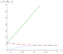
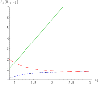
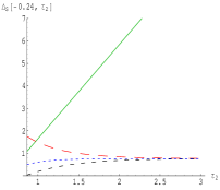
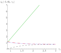
To investigate the relationship between the field and string predictions for the gauge field tadpoles further, we expand the string result as follows: As $\tau$ takes values within the fundamental domain ${\cal F}$, see figure 3, the exponential factor $\exp(-2\pi\tau_{2})<1$ always suppressed. The relevant exponentials for various small values of $\tau_{2}$ are given in table 5. Expanding the exact expressions for $\Delta_{s}(\tau,{\bar{\tau}})$ to order $\exp(-2\pi\tau_{2})$ gives

$$\begin{array}[]{lcl}\Delta_{u}(\tau,{\bar{\tau}})&=&-2\ln 3+4\pi\tau_{2}\frac{1}{3}+\ldots,\\[8.61108pt] \Delta_{t}(\tau,{\bar{\tau}})&=&\ln 3+6\cos(2\pi\frac{\tau_{1}}{3})e^{-2\pi\tau_{2}\,\frac{1}{3}}+9\cos(4\pi\frac{\tau_{1}}{3})e^{-2\pi\tau_{2}\,\frac{2}{3}}+\ldots,\\[8.61108pt] \Delta_{d_{+}}(\tau,{\bar{\tau}})&=&\ln 3+6\cos(2\pi\frac{\tau_{1}-1}{3})e^{-2\pi\tau_{2}\,\frac{1}{3}}+9\cos(4\pi\frac{\tau_{1}-1}{3})e^{-2\pi\tau_{2}\,\frac{2}{3}}+\ldots,\\[8.61108pt] \Delta_{d_{-}}(\tau,{\bar{\tau}})&=&\ln 3+6\cos(2\pi\frac{\tau_{1}+1}{3})e^{-2\pi\tau_{2}\,\frac{1}{3}}+9\cos(4\pi\frac{\tau_{1}+1}{3})e^{-2\pi\tau_{2}\,\frac{2}{3}}+\ldots.\end{array}$$ (28)

All these expressions are positive definite, as can inferred from their plots given in figure 4. As discussion in ref. [21] we have fixed the relative normal ordering constant between the untwisted and twisted world sheet bosons such that all $\Delta_{s}$ are strictly positive. This is important as allows us to Fourier transform the tadpole to coordinate space:

$$\langle F_{j{\underline{j}}}^{b}(z)\rangle=\frac{\delta^{4}(k_{4})}{(2\pi)^{4}}\,\sum_{s=u,t,d_{\pm}}\int_{\cal F}\frac{\mathrm{d}^{2}\tau}{\tau_{2}^{2}}\,Q_{s}^{b}(\tau)\,\Bigl{(}\frac{1}{\pi\Delta_{s}(\tau,{\bar{\tau}})}\Bigr{)}^{3}\,e^{-\bar{z}z/\Delta_{s}(\tau,{\bar{\tau}})}.$$ (29)

The resulting profiles for the different sectors are plotted in figure 5. We see that the twisted sector contributions $G_{t}$ and $G_{d_{\pm}}$ decay away very quickly for large $|z|$. Hence we see that the contributions of the twisted states are localized within a couple of string lengths near the orbifold singularity. The decay of the untwisted sector $G_{u}$ is much slower, as has been expected since the untwisted sector corresponds to bulk – non–localized – contributions.

file=LogCoorGauss.eps,width=8cm

Figure 5: The spatial extension of the tadpole contributions in the sectors $u,t$ and $d_{\pm}$ are displayed on a logarithmic scale. The curve for the $u$–sector fall off much slower than the others for large values of $|z|$, as only it corresponds to bulk contributions.

6 Local tachyons?

In the discussion of the previous section we have (implicitly) assumed that only the string zero modes contribute to the tadpoles. For the two heterotic $\mathrm{E_{8}}\times\mathrm{E_{8}}$ models with anomalous $\mathrm{U(1)}$’s this assumption is only true for the $\mathrm{SU(9)}$ model, given in table 2. For the other anomalous model, containing the $\mathrm{E_{7}}$ group, the situation is more complicated as can be seen from the charge functions:

$$\begin{array}[]{l}Q_{u}^{1}~{}~{}\approx~{}~{}3+\ldots,\\[4.30554pt] Q_{t}^{1}~{}~{}\approx~{}~{}\frac{1}{9}\,q^{-\frac{1}{3}}+\frac{5}{3}+6\,q^{\frac{1}{3}}-\frac{76}{9}\,q^{\frac{2}{3}}+\ldots,\\[4.30554pt] Q_{d_{+}}^{1}\approx~{}~{}\frac{1}{9}\,e^{i\frac{4\pi}{3}}\,q^{-\frac{1}{3}}+\frac{5}{3}+6\,e^{i\frac{2\pi}{3}}\,q^{\frac{1}{3}}-\frac{76}{9}\,e^{i\frac{4\pi}{3}}\,q^{\frac{2}{3}}+\ldots,\\[4.30554pt] Q_{d_{-}}^{1}\approx~{}~{}\frac{1}{9}\,e^{i\frac{2\pi}{3}}\,q^{-\frac{1}{3}}+\frac{5}{3}+6\,e^{i\frac{4\pi}{3}}\,q^{\frac{1}{3}}-\frac{76}{9}\,e^{i\frac{2\pi}{3}}\,q^{\frac{2}{3}}+\ldots,\end{array}$$ (34)

and

$$\begin{array}[]{l}Q_{u}^{2}~{}~{}\approx~{}~{}2+\ldots,\\[4.30554pt] Q_{t}^{2}~{}~{}\approx~{}~{}\frac{2}{9}\,q^{-\frac{1}{3}}-\frac{2}{3}+12\,q^{\frac{1}{3}}-\frac{152}{9}\,q^{\frac{2}{3}}+\ldots,\\[4.30554pt] Q_{d_{+}}^{2}\approx~{}~{}\frac{2}{9}\,e^{i\frac{4\pi}{3}}\,q^{-\frac{1}{3}}-\frac{2}{3}+12\,e^{i\frac{2\pi}{3}}\,q^{\frac{1}{3}}-\frac{152}{9}\,e^{i\frac{4\pi}{3}}\,q^{\frac{2}{3}}+\ldots,\\[4.30554pt] Q_{d_{-}}^{2}\approx~{}~{}\frac{2}{9}\,e^{i\frac{2\pi}{3}}\,q^{-\frac{1}{3}}-\frac{2}{3}+12\,e^{i\frac{4\pi}{3}}\,q^{\frac{1}{3}}-\frac{152}{9}\,e^{i\frac{2\pi}{3}}\,q^{\frac{2}{3}}+\ldots.\end{array}$$ (39)

The negative power $q^{-1/3}$ indicate that tachyonic states contribute to the charge functions $Q^{b}_{s}$ for the twisted sectors $s=t,d_{+}$ and $d_{-}$. (The positive powers result from massive string excitations. In fact, a tower of massive string states contribute to these local shapes.)

The presence of the tachyonic contributions is worrying, since it tachyons are normally taken as an indication of instabilities. But since the orbifold is supersymmetric it cannot be unstable. To understand what is going on, we consider the expression of the tachyonic contributions only in the coordinates space representation:

$${\cal T}(z)=\int_{\cal F}\frac{\mathrm{d}^{2}\tau}{\tau_{2}^{2}}\,e^{2\pi\,\frac{\tau_{2}}{3}}\left\{\cos\bigl{(}\frac{2\pi}{3}\tau_{1}\bigr{)}\Bigl{(}\frac{e^{-|z|^{2}/\Delta_{t}(\tau)}}{(\pi\Delta_{t}(\tau))^{3}}-{\cal E}_{+}(k|\tau)\Bigr{)}-\sqrt{3}\,\sin\bigl{(}\frac{2\pi}{3}\tau_{1}\bigr{)}{\cal E}_{-}(k|\tau)\right\}.$$ (40)

Like the exponential factor, the even and odd functions

$${\cal E}_{\pm}(z|\tau)=\frac{1}{2}\Bigl{(}\frac{e^{-|z|^{2}/\Delta_{d_{+}}(\tau)}}{(\pi\Delta_{d_{+}}(\tau))^{3}}\pm\frac{e^{-|z|^{2}/\Delta_{d_{-}}(\tau)}}{(\pi\Delta_{d_{-}}(\tau))^{3}}\Bigr{)},\qquad{\cal E}_{\pm}(z|-\tau_{1},\tau_{2})=\pm{\cal E}_{\pm}(z|\tau_{1},\tau_{2}),$$ (41)

contain the six dimensional Gaussian normalization factors $1/(\pi\Delta_{d_{\pm}})^{3}$. Therefore, the integral over the orbifold of each of these exponentials is normalized to unity. It follows that the integrated tadpole due to tachyons vanish. This implies the cancellation of the tachyonic contributions within the zero mode theory, which confirms that the model is globally stable.

file=CoorTachZeroLin.eps,width=9cm

Figure 6: The coordinate space representation of the tachyonic contributions to the gauge field tadpole is displayed by the solid line. This contribution dominates the largest zero mode contribution coming from the $d_{\pm}$ sectors.

In figure 6 the tachyonic contribution to the tadpole is plotted together with the leading contributions from the zero modes. Inspecting figure 5 we infer that the twisted sectors $d_{\pm}$ give the largest contributions to the zero mode states. (The other sectors contributions are at least one order of magnitude less, and can therefore safely be ignored in the present analysis.) The normalization of the zero modes in the $d_{\pm}$ sectors compared to the tachyonic sector is $15$ and $-3$ for the first and second $E_{8}$, respectively, see equations (34) and (39). These relative normalizations have been taken into account in comparison figure 6. We conclude that the tachyonic states totally dominate the profile of the tadpoles for the $\mathrm{U(1)}$’s in both $\mathrm{E_{8}}$’s near the singularity.

This curious appearance of local tachyonic contributions to gauge field tadpoles does not only appear in the heterotic $\mathrm{E_{8}}\times\mathrm{E_{8}}$ theory, but is also present in some $\mathrm{SO(32)}$ string models. There are five heterotic $\mathrm{SO(32)}$ models $\mathbb{Z}_{3}$ classified according to their gauge shift vector $v=(1^{2n},-2^{n},0^{16-3n})/3$, $n=1,\ldots 5$, with an anomalous $\mathrm{U(1)}$. In the $n=2$ and $5$ models local tachyons are present as well, while in the others, like the $\mathrm{SU(9)}$ model, only zero modes contribute to the tadpole. The full implications of these local tachyons have not been uncovered yet and might provide an interesting avenue for future research.

7 Conclusions

We began this review by considering field theories on orbifolds. Even though such theories have many useful and interesting properties, the physics near the orbifold singularity is beyond the realm of field theory. To investigate just how far one can push the field theory analysis we compute gauge field tadpoles on a $\mathbb{Z}_{3}$ orbifold and found singular behavior near the orbifold fixed point where the field theory calculation might not be trusted. We considered heterotic string models as UV completions of the field theory and computed the gauge field tadpoles in this framework as well. Away from the orbifold singularity the qualitative properties of both computations are the same. Near the orbifold singularity things are different. In particular, the twisted states which in field theory are assumed to be localized exactly at the orbifold fixed point, have in string theory a finite extend of a couple of string lengths. Moreover, contrary to the field theory result, string theory gives strictly finite answer.

These string results could have been anticipated, what has been a major surprise of our computation of the gauge field tadpoles in string theory is that for some orbifold models there are, aside from the zero modes, contributions from local tachyonic states to these amplitudes. Yet, these tachyons do not signify a global instability since they are not present in the spectrum of the theory, contributing only in the loop. Moreover, when integrated over the whole orbifold, these tachyonic contributions precisely cancel each other.

References

• [1] P. Fayet and J. Iliopoulos Phys. Lett. B51, 461–464 (1974).
• [2] W. Fischler, H. P. Nilles, J. Polchinski, S. Raby, and L. Susskind Phys. Rev. Lett. 47, 757 (1981).
• [3] M. Dine, N. Seiberg, and E. Witten Nucl. Phys. B289, 589 (1987).
• [4] J. J. Atick, L. J. Dixon, and A. Sen Nucl. Phys. B292, 109–149 (1987).
• [5] M. Dine, I. Ichinose, and N. Seiberg Nucl. Phys. B293, 253 (1987).
• [6] E. Poppitz Nucl. Phys. B542, 31–44 (1999) [hep-th/9810010].
• [7] E. A. Mirabelli and M. E. Peskin Phys. Rev. D58, 065002 (1998) [hep-th/9712214].
• [8] D. M. Ghilencea, S. Groot Nibbelink, and H. P. Nilles Nucl. Phys. B619, 385–395 (2001) [hep-th/0108184].
• [9] R. Barbieri, L. J. Hall, and Y. Nomura [hep-ph/0110102].
• [10] C. A. Scrucca, M. Serone, L. Silvestrini, and F. Zwirner Phys. Lett. B525, 169–174 (2002) [hep-th/0110073].
• [11] S. Groot Nibbelink, H. P. Nilles, and M. Olechowski Phys. Lett. B536, 270–276 (2002) [hep-th/0203055].
• [12] S. Groot Nibbelink, H. P. Nilles, and M. Olechowski Nucl. Phys. B640, 171–201 (2002) [hep-th/0205012].
• [13] H. M. Lee, H. P. Nilles, and M. Zucker Nucl. Phys. B680, 177–198 (2004) [hep-th/0309195].
• [14] R. Barbieri, R. Contino, P. Creminelli, R. Rattazzi, and C. A. Scrucca Phys. Rev. D66, 024025 (2002) [hep-th/0203039].
• [15] D. Marti and A. Pomarol Phys. Rev. D66, 125005 (2002) [hep-ph/0205034].
• [16] G. von Gersdorff, N. Irges, and M. Quiros Phys. Lett. B551, 351–359 (2003) [hep-ph/0210134].
• [17] C. Csaki, C. Grojean, and H. Murayama Phys. Rev. D67, 085012 (2003) [hep-ph/0210133].
• [18] S. Groot Nibbelink, H. P. Nilles, M. Olechowski, and M. G. A. Walter Nucl. Phys. B665, 236–272 (2003) [hep-th/0303101].
• [19] S. Groot Nibbelink and M. Laidlaw JHEP 01, 004 (2004) [hep-th/0311013].
• [20] J. Polchinski Commun. Math. Phys. 104, 37 (1986).
• [21] S. Groot Nibbelink and M. Laidlaw JHEP 01, 036 (2004) [hep-th/0311015].
• [22] I. Antoniadis, E. Kiritsis, and J. Rizos Nucl. Phys. B637, 92–118 (2002) [hep-th/0204153].