Abstract

We present supersymmetric, tadpole-free $d=4,N=1$ orientifold vacua with a three family chiral fermion spectrum that is identical to that of the Standard Model. Starting with all simple current orientifolds of all Gepner models we perform a systematic search for such spectra. We consider several variations of the standard four-stack intersecting brane realization of the standard model, with all quarks and leptons realized as bifundamentals and perturbatively exact baryon and lepton number symmetries, and with a $U(1)_{Y}$ vector boson that does not acquire a mass from Green-Schwarz terms. The number of supersymmetric Higgs pairs $H_{1}+H_{2}$ is left free. In order to cancel all tadpoles, we allow a “hidden” gauge group, which must be chirally decoupled from the standard model. We also allow for non-chiral mirror-pairs of quarks and leptons, non-chiral exotics and (possibly chiral) hidden, standard model singlet matter, as well as a massless B-L vector boson. All of these less desirable features are absent in some cases, although not simultaneously. In particular, we found cases with massless Chan-Paton gauge bosons generating nothing more than $SU(3)\times SU(2)\times U(1)$. We obtain almost 180000 rationally distinct solutions (not counting hidden sector degrees of freedom), and present distributions of various quantities. We analyse the tree level gauge couplings, and find a large range of values, remarkably centered around the unification point.

1 Introduction

String theory is hoped to be a consistent theory of quantum gravity, with the special feature that it strongly constrains the matter it can couple to. Although direct experimental tests of new predictions seem out of reach for the moment, it can at least be tested theoretically by verifying its internal consistency, in particular with regard to gravity, and by checking that the limited set of matter it can couple to includes the standard model. We may be lucky enough that the way the standard model is embedded in string theory implies predictions for future experiments, but it may also happen that using all known experimental constraints we are still left with more than one, or even a huge number of possibilities. But at present it is still a serious challenge to find even one “string vacuum” (which may actually be a metastable, approximate ground state) that is a credible standard model candidate. To find such a vacuum requires an in-depth analysis of known candidates based on robust criteria derived from experiment. However, even within the known classes of vacua, large areas have remained unexplored so far. As longs as that is the case, nature would have to be very kind to us to allow us to find the ground state on which our universe is based. In this paper we want to make a modest step towards broadening the set of accessible vacua, by means of a systematic exploration of orientifolds of Gepner models. It turns out that this class is very rich, and includes an abundance of standard model-like spectra far beyond anything that has come out of string theory so far. Some early, and partial results were reported in [1].

Since 1984 there have been several attempts to search for standard model like string vacua. Two general classes may be distinguished: heterotic string constructions (either (2,2) or (0,2)), with the standard model particles realized as closed strings, and type-I (orientifold, intersecting brane) constructions, characterized by open string realizations of the standard model. Other possibilities certainly exist (e.g. M-theory compactifications), and since new ways of obtaining the standard model are discovered about every five to ten years, it might be an illusion to think that we are close to a complete picture.

To explore the two classes mentioned above, we have essentially three methods at our disposal: free CFT constructions (free bosons and/or fermions and orbifolds thereof), geometric compactification (in particular Calabi-Yau compactifications) and interacting CFT constructions. All three have been applied successfully to heterotic string construction. The earliest example [2] of a three-family model was based on the Tian-Yau Calabi-Yau manifold with Euler number 6 and a non-trivial homotopy group $\pi_{1}$ (as far as we know still the only known manifold of this kind), used for Wilson line symmetry breaking. About a year later, the first orbifold examples were found [3, 4] (see also [5] for later developments). In [6] a three-family model was constructed using tensor products of $N=2$ minimal models, corresponding to a point in the moduli space of the Tian-Yau manifold. This model has an $E_{6}$ gauge group. By reducing the $(2,2)$ world-sheet symmetry to $(0,2)$ a large number of related models was constructed in [7] with $E_{6}$ or $SO(10)$ gauge symmetry. The symmetry in the bosonic sector can be reduced further to obtain many models with a gauge group $SU(3)\times SU(2)\times U(1)\times[\hbox{Other factors}]$ and three families of quarks and leptons [8]. Another class of three family models was obtained using free fermions in [9, 10, 11], and extended in [12]. By means of a modified Calabi-Yau construction yielding $(0,2)$ spectra, several more three-family models were obtained in[13]. All the foregoing models lead to level 1 realizations of the standard model gauge groups $SU(3)$ and $SU(2)$, and hence their spectra contain fractionally charged states, or they have a non-standard normalization for the standard model $U(1)$ generator (or both) [14, 15, 16]. Unified models with standard model charge quantization can be constructed by using higher level Kac-Moody algebras, and indeed three family models were obtained [17]. Yet another approach to getting the standard model, based on strongly coupled heterotic strings, was presented in [18]. All of these heterotic three family models are supersymmetric. Constructing non-supersymmetric heterotic strings is much easier, but those theories are not stable, in general.

The open string road towards the standard model has been considerably more difficult. Until about 1995 this option was rarely taken seriously, with a few exceptions [19, 20]. This changed after the discovery of D-branes [21] and the observation in [22] that the problematic relation between the unification scale and the Planck scale could be avoided in open string theories. The construction of realistic theories is complicated by several new features, on top of those of the closed type-II theory to which the orientifold procedure is applied: boundary and crosscap states and the requirement of tadpole cancellation. The first four-dimensional chiral, supersymmetric theory was constructed in [23], but it was still far from realistic. In order to get standard model-like spectra, in several later papers (e.g. [24, 25, 26, 27, 28, 29, 30, 31, 32]) the requirement of supersymmetry was relaxed, and only part of the the tadpoles were cancelled, namely the RR tadpoles needed for consistency. The resulting theories are not stable, but otherwise consistent. The first semi-realistic supersymmetric theory that satisfies all tadpole conditions was presented in [33] and [34, 35]. However, these spectra contains chiral exotics, in addition to the standard model representations. In [36, 37] a three family supersymmetric Pati-Salam ($SU(4)\times SU(2)\times SU(2)$) model was constructed, but the two $SU(2)$s do not emerge directly from string theory but from a diagonal subgroup of Chan-Paton groups using a “brane recombination” mechanism. In [38] supersymmetric Pati-Salam models were found that emerge directly from the CP-groups, but with additional chiral exotic matter, and in [39] supersymmetric $SU(5)$ GUT models with chiral exotics were presented. Most of the foregoing constructions are based on orientifolds of of toroidal orbifolds [40, 41], except for [29] which uses the quintic Calabi-Yau manifold. In [42] standard model like spectra where obtained using branes at singularities. The first investigation of string spectra from open strings of orientifolds of Gepner models was done in [43], in 6 dimensions. The first analysis in four dimensions was done by [44]. These authors did not find chiral spectra, but got a first glimpse of the vast landscape of solutions. Further work on this kind of construction, including some chiral spectra, was presented in [44, 45, 46, 47, 48, 49, 50]. In [1], the precursor of the present paper, the first examples were found of supersymmetric standard model spectra, with the standard model group appearing directly as a Chan-Paton group and without chiral exotics. Shortly thereafter the first such example was found in the context of orientifolds of toroidal orbifolds [51]. In [52, 53] the first semi-realistic examples were found with flux comapctifications and partially stabilized moduli, although with chiral exotics. For recent results on chiral fermions from Gepner orientifolds see [50]. For recent reviews with more references consult for example [54, 55, 56, 57].

Recently there has been a lot of work on (non)-supersymmetric vacua with moduli stabilized by three-form fluxes on a Calabi-Yau manifold. Although this is an extremely interesting development, we will not consider it here, simply because the methods we use do not allow this at present.

For a variety of reasons we will require the string spectrum to be supersymmetric. The first reason is phenomenological. Although we do not commit ourselves to a supersymmetry breaking mechanism or scale, the most obvious scenario is the standard one: supersymmetry breaking at a few TeV, induced by gaugino condensation in a hidden sector (which exists in most of our models), with supersymmetry playing the role of protecting the gauge hierarchy. Indeed, such a hierarchy inevitably exist in these models, since six dimensions are compactified on a Calabi-Yau manifold at a rational point in moduli space, and hence there is no reason to expect some of the compactified dimensions to be extremely large. There are two other reasons why we want to keep supersymmetry unbroken. First of all, we can then be certain that the four-dimensional strings we construct are stable and consistent. But the most important reason is a practical one. Space-time supersymmetry has the effect of extending the world-sheet chiral algebra, thereby organizing the fields into a smaller number of primaries. This is what makes our computations manageable in practice.

The use of rational conformal field theory (RCFT) in these constructions has well-known advantages and disadvantages. The advantage of the algebraic approach is that we can explore a large class of models with uniform methods. But clearly the disadvantage is that one ends up in a special point in moduli space, both with regard to the Calabi-Yau manifold, as well as the choice of branes wrapping it. It is not reasonable to expect such a ground state to be exactly the standard model, because many observable quantities, such as quark and lepton masses and gauge couplings will depend on the moduli, which have been fixed at a specific value. Clearly we should focus on those features that do not depend on the moduli. The primary feature to consider is then of course the chiral spectrum.

Apart from supersymmetry breaking there are several other important issues that we do not consider here, such as standard model symmetry breaking, Yukawa couplings, Majorana masses for the neutrinos, etc. We see our results therefore mainly as a first exploration of some interesting regions in the huge landscape of possible models. Once a promising type of model has been identified, one may try to explore it in more detail, either by CFT perturbations in the neighborhood of the special point, or by constructing the corresponding Calabi-Yau and the set of branes on it, using the RCFT results as a guideline. Even within the context of RCFT one could push these models further and compute certain couplings, but unfortunately the required CFT techniques are not yet available for all couplings. For example, three-point couplings between open strings are in principle computable in RCFT, but to develop this formalism to include non-trivial modular invariant partition functions and simple current fixed points would still require a substantial amount of work. Gauge couplings, on the other hand, are easily computable, and we do so in all cases.

Since we end up with a very large set of solutions, our results should give a reasonable idea of what kind of spectra one may expect, and one can perform some statistical analysis on this set, somewhat similar in spirit (though with a quite different philosophy) to the approach presented in [58]. In addition, despite the inherent limitations of the algebraic approach, one may explore the effect of brane moduli as well as some Calabi-Yau moduli. The former, since for a given CY-manifold we typically find a large number of spectra, which can be interpreted in terms of branes in different discrete positions; the latter, because some distinct Gepner points may lie on the same Calabi-Yau moduli space. Especially the brane position moduli seem to be probed rather effectively by rational points, in certain cases.

1.1 Brane configurations considered

In this paper we consider boundary states in a rational type IIB CFT. The relevant physical open string quantities are annulus and Moebius coefficients. For the sake of clarity, it is convenient to present the models in terms of an intersecting brane picture, although such a picture is not really used in our construction. This picture would be appropriate in a large volume limit and for type IIA string, the mirror of what we consider here. The geometric interpretation of the construction considered here is presumably in terms of magnetized D3 and D7 branes [24]. In the following, by the “intersection” of two branes a and b we mean $\sum_{i}A^{i}_{ab}\chi^{i}(\tau/2)|_{0}$, where $A^{i}_{~{}ab}$ is an annulus coefficient and $\chi$ is the character restricted to massless states. By the “chiral intersection” we mean the same quantity restricted to chiral states.

We consider here a specific type of intersecting brane models, based on a four-stack configuration with a baryon brane, a weak brane (or left brane), a right brane and a lepton brane, labeled a,b,c,d respectively [26]. These are the minimal brane configurations with baryon and lepton number conservation and all quarks and leptons realized as bifundamentals. The Chan-Paton gauge groups associated with these branes contain the standard model gauge group. In addition we allow “hidden branes”, with gauge groups with respect to which all standard model particles are neutral. These branes were introduced to cancel massless tadpoles, but their gauge groups may play a useful phenomenological rôle, in particular for gaugino condensation.

The a and d branes are required to be complex, and carry Chan-Paton group $U(3)_{\rm a}$ and $U(1)_{\rm d}$ respectively. The former contains the standard model gauge group $SU(3)$. The overall phase factor of $U(3)_{\rm a}$ corresponds to baryon number, and the $U(1)_{\rm d}$ to lepton number. In the standard model these symmetries are not gauged, and anomalous. In string theory these anomalies are canceled by Green-Schwarz terms, involving a bilinear coupling of the “bary-photon” and “lepto-photon” to massless two-form fields. These couplings produce a mass for the linear combination $B+L$ of these $U(1)$ bosons, breaking the corresponding combination of baryon and lepton number. Nevertheless the broken symmetry still prevents the appearance of dangerous baryon and lepton number violating couplings at least perturbatively [26].

The b and c branes may be real or complex. In the standard four-stack realization of the standard model the first family emerges as follows if they are both complex, with CP-groups $U(2)_{\rm b}$ and $U(1)_{\rm c}$ respectively

$$(u,d): [{\rm a},{\rm b}]\hbox{ or }[{\rm a},{\rm b}*]$$ (1)

$$u^{c}: [{\rm a}^{*},{\rm c}]$$ (2)

$$d^{c}: [{\rm a}^{*},{\rm c}^{*}]$$ (3)

$$(e^{-},\nu): [{\rm b},{\rm d}]\hbox{ or }[{\rm b}^{*},{\rm d}]$$ (4)

$$e^{+} [{\rm c},{\rm d}^{*}]$$ (5)

$$\nu^{c}: [{\rm c}^{*},{\rm d}^{*}]$$ (6)

Here $[x,y]$ denote strings beginning on brane $x$ and ending on brane $y$, and $x^{*}$ is the brane conjugate to $x$. The $Y$-charge of the standard model is given by the linear combination

$$Y=\frac{1}{6}Q_{\rm a}-\frac{1}{2}Q_{\rm c}-\frac{1}{2}Q_{\rm d}\ .$$

The overall phase symmetry in $U(2)_{\rm b}$ is always anomalous with respect to the $a$ and the $d$ branes and the corresponding gauge boson acquires a mass; the surviving gauge group is $SU(2)_{W}$. Note that $B+L$ and $U(2)_{\rm b}$ have independent anomalies with respect to the standard model, so that there is no linear combination of these phases symmetries that remains unbroken.

The standard model weak gauge group can also be constructed out of real branes on top of an orientifold plane, yielding $Sp(2)$. Since the spectrum is real with respect to the c-brane, we may allow the group $O(2)_{\rm c}$ here instead of $U(1)_{\rm c}$, with $Q_{\rm c}$ replaced by the (properly normalized) $O(2)$ generator in the definition of the charge. Since $O(2)$ branes differ from $Sp(2)$ branes only by a Moebius sign, we decided to allow the latter as well. Strictly speaking this is a departure from our philosophy of looking only for the simplest standard model realizations, but these models are as easy to look for as $O(2)$ models, and have the interesting feature of yielding “left-right symmetric” models with an $SU(2)_{L}\times SU(2)_{R}$ gauge group. Such gauge groups appear as part of the symmetry-breaking chain of the Pati-Salam model, and indeed in some examples there are related spectra with the $d$ brane on top of the $a$ brane, yielding precisely the Pati-Salam model. Then we end up with following six types of models:

Type 0 $$\;U(3)\times Sp(2)\times U(1)\times U(1)$$

Type 1 $$\;U(3)\times U(2)\times U(1)\times U(1)$$

Type 2 $$\;U(3)\times Sp(2)\times O(2)\times U(1)$$

Type 3 $$\;U(3)\times U(2)\times O(2)\times U(1)$$

Type 4 $$\;U(3)\times Sp(2)\times Sp(2)\times U(1)$$

Type 5 $$\;U(3)\times U(2)\times Sp(2)\times U(1)$$

The complete spectrum of these theories can contain massless vector bosons from three sources: the standard model part of the open sector, as listed above, additional “hidden” branes, and the closed sector. The latter gauge bosons are nearly inevitable, but do not have minimal couplings to the quarks and leptons. The gauge bosons from the hidden sector may be absent altogether, but in any case do not couple to the standard model particles. If we ignore these two kinds of vector bosons, the gauge group is quite close to that of the standard model. As a Lie-algebra, it is a non-abelian extension of the standard model only for types 4 and 5; in all other cases we get the standard model with at most one additional non-anomalous $U(1)$ factor, $B-L$.

The gauge bosons coupling to the non-anomalous symmetries $Y$ and $B-L$ can acquire a mass from Green-Schwarz type two-point couplings to two-form fields, provided that these couplings do not generate a contribution to the anomaly. We find that in most cases such a mass contribution is absent, and that $Y$ is more likely to acquire a mass than $B-L$. The latter statement is based only on the models presented in [1], where masslessness of $Y$ was only used as an a posteriori check. In the present paper brane stacks yielding non-zero $Y$-mass were eliminated before attempting to solve the tadpole equations, but no condition was imposed on the $B-L$ mass. We found a massive $B-L$ photon in about $3\%$ of the type-0 models, and for none of the type-1 models (of which we found only very few). There are even models with a massive $B-L$ and no extra branes at all. These models (22in total) have precisely the standard model gauge group from the open sector, but there are still 18 additional Ramond-Ramond vector bosons from the closed sector.

We expect masslessness of the Y-boson, in addition to lepton and quark chirality and supersymmetry, to be among the features of these models that are unaffected by generic perturbations around the rational point. The potential origin of a Y-boson mass would be the generation of a two-point coupling to one of the RR two-forms away from the rational point. However, such a two-point coupling would very likely generate an anomalous contribution in combination with a three-point coupling of the same RR-two form to two gauge bosons.

The same logic applies to the $B-L$ gauge boson. If it is massless at the string level, it should acquire a mass trough a fundamental or dynamical Higgs mechanism, just as the $Z$ and $W$ bosons. Candidates for the required Higgses are the sneutrinos or two standard model/ hidden sector bifundamentals (one ending on the c-brane and one on the d-brane), bound by a hidden sector gauge group.

Most other features cannot be expected to survive generic perturbations. In particular this concerns the massless particles that are non-chiral with respect to $G_{\rm S}$, namely the mirrors, rank-2 tensors, leptoquarks and standard model/hidden sector bifundamentals. It seems plausible that for many of them masslessness is an artifact of being in a rational point in moduli space. They will get a mass when the moduli are changed, and one can investigate this by computing the coupling of the closed string moduli to the massless fermions. However, some of the massless particles correspond to brane position moduli, and hence to flat directions in the superpotential. One of the problems we have in investigating this and other more detailed phenomenological issues is that we have to find a way to do a meaningful analysis for a huge number of solutions.

There are many other brane configurations that would yield standard-model-like spectra. For example another attractive possibility might be to start with a $U(5)$ stack (realizing an $SU(5)$ GUT) plus other branes or the reduction of such a stack to $U(3)\times U(2)$. In such models some quarks and leptons emerge as anti-symmetric tensors and baryon and lepton number are not symmetries. Models of this type were studied in [39], but so far with the disappointing result that there are additional chiral symmetric tensors of $SU(5)$. In principle one could search for models of this kind in exactly the same way, just as one could search for Pati-Salam type models. It goes without saying that if we were to relax some constraints and allow for example chiral exotics or diagonal embeddings of standard model factors in the CP group, then the number of solution would almost certainly explode. Nevertheless such options, although unattractive, are not necessarily ruled out experimentally.

1.2 Chirality

Let us explain more precisely what we mean by “getting the standard model from string theory”, since this issue tends to cause confusion. Quite generally, one might accept any string spectrum if the gauge group $G_{\rm S}$ emerging directly from open or closed strings contains $G_{\rm SM}=SU(3)\times SU(2)\times U(1)$, and if the fermion representation of $G_{\rm S}$ reduces to three times $(3,2,\frac{1}{6})+(3^{*},1,\frac{1}{3})+(3^{*},1,-\frac{2}{3})+(1,2,-\frac{1}{2})+(1,1,1)$, written in terms of left-handed Weyl fermions. These should be the only fermions that are chiral with respect $SU(3)\times SU(2)\times U(1)$. If at this stage there were additional chiral particles one could still imagine mechanisms that give them a sufficiently large mass after standard model symmetry breaking and $SU(3)$ confinement, but if that were true we simply need more experimental input to go ahead. There may be additional massless fermions that are non-chiral with respect to $SU(3)\times SU(2)\times U(1)$ and their may be additional fermions, chiral with respect to $G_{\rm S}$, that become non-chiral after the reduction from $G_{\rm S}$ to $SU(3)\times SU(2)\times U(1)$.

The group $G_{\rm S}$ is the complete CP-group from the open sector times any gauge group generated by closed sector vector bosons. The physical realization of the group theoretical “reduction” mentioned above can take many forms, such as mass generation for $U(1)$’s by Green-Schwarz anomaly cancelling terms, confinement or breaking by a fundamental or dynamical Higgs effect. Furthermore part of $G_{\rm S}$ may remain unbroken, if the corresponding gauge bosons do not couple to quarks and leptons. We did not commit ourselves here to a particular reduction mechanism. In the majority of the spectra we consider, $G_{\rm S}$ is embedded in $G_{\rm SM}$ as $G_{\rm S}=G_{\rm SM}\oplus G_{\rm Hidden}$ (as a Lie-algebra), except in types 4 and 5, where the $U(1)_{\rm c}$ group is non-trivially extended to $Sp(2)$. In the latter cases an additional Higgs-like mechanism would be required to arrive at the standard model. Just as is the case with the supersymmetry breaking and the standard model Higgs mechanism, one could impose additional constraints on the results in order for a a particular mechanism to be realized, but such constraints are less robust and more model-dependent than the requirement of chirality, our main guiding principle.

The possibilities for $G_{\rm S}$-chiral particles that are $G_{\rm SM}$-non-chiral are the following

1. Right-handed neutrinos. These particles are singlets (and hence not chiral) w.r.t. $G_{SM}$ but are chiral with respect to lepton number, which is broken. In our case, there are always three of them. This is an inevitable consequence of tadpole cancellation, which cancels the cubic anomalies in $U(1)_{\rm d}$, plus the fact that we only allow bifundamentals of the (a,b,c,d) branes to be chiral.

2. Higgsinos. In the MSSM the fermionic partners of the Higgs are non-chiral with respect to $G_{SM}$, but in models of types 1, 3 and 5 there is a possibility for the Higgses to be chiral with respect to $U(2)_{\rm b}$. This gauge symmetry breaks to $SU(2)$ in the first step, but its initial presence can still forbid the generation of large masses for the Higgs. This is a desirable feature, as it may give a mechanism for getting light Higgs bosons.

3. Mirror quarks and leptons, which are chiral with respect to $U(2)_{\rm b}$. These particles can appear for the same reason as the Higgsinos, but are less desirable. For example the $U(3)\oplus U(2)$ combinations $(3,2)+(3^{*},2)$ is chiral, but becomes non-chiral when $U(2)_{\rm b}$ is reduced to $SU(2)$. We have allowed such particles in principle, but (just as the chiral Higgsinos), they occur only rarely.

4. $G_{SM}$ singlets, which are chiral with respect to the hidden gauge group. Such particles couple only the the SM-matter gravitationally, and hence are acceptable as “dark matter”, if not too abundant. Furthermore they may acquire a mass and/or be confined by $G_{\rm Hidden}$ dynamics.

Unwanted chiral matter within the standard model sector can be avoided by the selection of a,b,c and d branes, and chiral matter from open strings stretching between the SM branes and the hidden branes can be avoided by appropriate selection of the latter. One could in principle also forbid chiral rank-2 tensors within $G_{\rm Hidden}$ by an a priori constraint, but it is very hard to forbid chiral bifundamentals within $G_{\rm Hidden}$, except by constructing all solutions and eliminating them a posteriori. Since constructing all solutions is nearly impossible in most cases, we decided to allow $G_{\rm SM}$-singlets that are chiral with respect to $G_{\rm Hidden}$. Nevertheless, they occur in only a small fraction (about 12.5%) of our solutions. This is largely due to the fact that our search is biased in favor of few additional branes, and it is harder to make chiral spectra with fewer branes, and impossible with a single brane.

1.3 Scope of the search

In this paper we consider all modular invariant partition functions (MIPFs) that are symmetric simple current modifications of the charge conjugation invariant of all 168 minimal N=2 tensor products. The precise number of such MIPFs is determined as follows. Generically, it is just a matter of applying the procedure of [59, 60] and restricting to symmetric bi-homorphisms $X$ (defined more precisely in [60] and in the next chapter). However, if there are identical N=2 factors in the tensor product, there will be equivalences among these MIPFs, and we remove equivalent ones. Furthermore, for small values of $k$ (the “level” of the minimal model), especially $k=2$, generically distinct simple current invariants are in fact identical, and these are also removed from the set. We then end up with 5403 distinct MIPFs. They can be characterized in part by the resulting Hodge numbers $h_{11}$ and $h_{21}$, and by the number of gauge singlets in the heterotic string spectrum. These numbers can be compared to tables of such spectra produced about fifteen years ago [7, 61]. Unfortunately a complete comparison is difficult, because the old results are either no longer available, and certainly not in electronic form, or the search was not fully exhaustive, or the symmetry of the MIPFs was not specified. But to the extent that a comparison is possible the results seem to agree.

In a few cases there appear to be further equivalences, or at least some MIPFs may correspond to distinct rational points on the same Calabi-Yau space. In total we found 873 different combinations of Hodge numbers, and 1829 Hodge numbers plus singlets (i.e gauge singlets in the Heterotic spectrum.)

For each of these MIPFs we consider all orientifolds allowed by the general formula of [62]. These orientifolds are subject to three equivalence relations, one originating from permutations of identical factors, and two as part of the general formalism. These equivalences are removed, and we then end up with a total of 49322 a priori distinct orientifolds. Our results indicate that indeed they are generically distinct.

For each MIPF and orientifold we consider the complete set of boundaries. This means that the number of boundaries is equal to the number of Ishibashi states of the MIPF. The MIPF may be of any type: pure fusion rule automorphisms, extensions of the chiral algebra, or combinations thereof. The beauty of the formalism of [62] is that it works independently of such details. It is well-known that in the case of extensions one can distinguish boundaries that respect the extended symmetry and boundaries that do not. A complete set of boundaries contains both kinds. The CFT we start with is itself an extension of the minimal model tensor product CFT (by alignment currents and the space-time supersymmetry current). Those extensions are respected by all our solutions, by construction. If the MIPF extends the chiral algebra further, one could work directly in the extended CFT and only consider boundaries that respect the extension. One would then find a subset of our solutions. Alternatively, one could also start with less symmetry, and treat for example space-time supersymmetry as a bulk extension. This would allow, in principle, supersymmetry breaking boundaries. In practice this is quite hard, because the number of primary fields increases dramatically. Undoubtedly, so will the number solutions.

Our goal was to complete this analysis for all MIPFs, in order to arrive at a picture that is as complete as possible. Unfortunately, the analysis could not be completed in all cases. Two tensor combinations had too many primaries to finish the computation of chiral intersections in a reasonable amount of time. In five others the number of candidate (a,b,c,d) branes was so large that we decided to restrict ourselves to types 0 and 1, of which there are fewer. For a given MIPF, orientifold and type, the number of four-stack candidates was more than a million in some cases.

The main computational stumbling block are the tadpole equations. For every valid set of (a,b,c,d) branes, the number of variables is equal to the number of boundaries that do not have a chiral intersection with a,b,c and d. This number can become as large as several hundreds, for a few tens of tadpole equations. Obviously, the time needed to evaluate this completely grows exponentially with the surplus of variables over equations. This means that beyond a certain number of variables it is impossible to decide conclusively that there are no solutions. In those cases we did perform a systematic search for solutions with 0,1 and 2 hidden branes, and 3 if the number of variables was less than 100, 4 if the number was less than 400. Furthermore, in the simpler cases we attempted solving the equations in general. Of the 5403 MIPFs, 2 were not analysed at all, and 20 only for types 0 and 1, and in 495 cases the tadpole equations were not fully analysed (153 of these did have solutions, however).

There are several possible ways to count solutions as distinct. On the one hand, one could regard solutions as identical if they are connected to each other by continuous, non-singular variations of open or closed string moduli. In an RCFT approach this is hard to do, since we cannot vary the moduli in a continuous way. The other extreme would be to count all distinct massless spectra, including the hidden sector gauge groups and representations. This is also not possible in our case, since we did not do a systematic search through all hidden sector gauge groups. We have chosen an intermediate criterium: solutions are regarded as distinct if they are of different type or have a different massless (chiral and non-chiral) standard model spectrum. Furthermore we treat different dilaton couplings for the a,b,c,d branes and the O-plane as a distinction, and the absence or presence of a hidden sector. By contrast, in [1] hidden sector distinctions were also counted. The number of solutions for one of the MIPFs of the tensor product $(6,6,6,6)$ quoted in that paper (“more than 6000”) reduces to 820 with our present way of counting.

1.4 Contents

This paper is organized as follows. In the next chapter, we review the ingredients of the algebraic orientifold construction. Section 3 contains a general discussion of the massless spectrum. In section 4 we discuss tadpole and anomaly cancellation. Chapter 5 contains our results. Due to the huge number of solutions it is impossible and pointless to present detailed spectra. Therefore we only give distributions of several quantities of interest, such as the number of Higgs scalars. We also analyse the values of gauge coupling ratios at the string scale. In section 6 we present one example in more detail, a model without any additional branes that in several respects is the simplest we encountered. In section 7 we formulate some conclusions. An essential computational technique is to organize the Ishibashi and boundary labels into simple current orbits, which leads to a dramatic speed-up of the calculations. This is explained in the appendix.

2 Algebraic Model Building

Our starting point is four-dimensional type-II string obtained by tensoring NSR fermions with a combination of N=2 minimal models with total central charge 9. In a covariant description, the NSR part of the theory is built out of four fermions $\psi^{\mu}$ with Minkowski metric, and a set of superconformal ghosts. The type-II theory is modular invariant and has two world-sheet supersymmetries needed for consistency. We assume it to be symmetric in left- and right-moving modes and have an extended chiral algebra leading to two space-time supersymmetries. To this theory we apply the orientifold procedure. Since our approach is based on unitary rational CFT, it is convenient to use this description not only for the minimal N=2 factors, but also for the NSR part of the theory. To do so we use a bosonic description of the latter (see [63] and references therein). This is convenient because model-independent complications due to the GSO projection, spin-statistics and superconformal ghosts are automatically taken care of. This implies that we are formally constructing bosonic open strings. To obtain the spectrum we mimic the procedure used in the covariant approach, namely fix a ghost charge to select the physical states. This translates into a consistent truncation of the bosonic string characters. In the case of closed strings, this procedure can be shown to map modular invariant bosonic strings to modular invariant fermionic strings. In the case of open strings, it leads to fermionic open strings satisfying all the integrality conditions on torus and Klein bottle as well as Annulus and Möbius strip amplitudes, and that have the correct spin-statistics for all physical states, and the proper symmetrization for Ramond-Ramond states. We emphasize that this is only used here as a bookkeeping device, and that we are not trying to conjecture a relation between fermionic and bosonic strings.

Our starting point is a class of bosonic string theories with chiral algebra

$$E_{8}\otimes D_{5}\otimes{\cal A}_{int}\;\;\;,$$ (8)

where $E_{8}$ and $D_{5}$ are level 1 affine Lie algebras models. In this paper we can take the model-dependent factor ${\cal A}_{int}$ to be of $4d$ Gepner type

$${\cal A}_{int}=\otimes_{k=1}^{r}{\cal A}_{k}\;\;\;,\;\;\;c_{int}=9$$ (9)

and ${\cal A}_{k}$ is the $N=2$ minimal model at level $k$. The $E_{8}$ factor has no influence on the massless spectrum. The only role of this factor is to cancel the conformal anomaly $c_{8}+c_{5}+c_{int}+c_{bos}+c_{ghosts}=8+5+9+4-26=0$ where $c_{bos}$ is the contribution of the uncompactified bosons. The $D_{5}$ factor describes the lightcone NSR fermions plus the longitudinal NSR fermions and superconformal ghosts. The truncation that we implement at the end of the day basically amounts to removing the contribution of the latter. For the construction of the type-II string we follow the procedure explained in [7] (see also [64]) for heterotic strings, the only difference being that the fermionic truncation is applied to both the left- and the rightmoving sector. The tensor product (8) is first extended by means of alignment currents (even combinations of the world-sheet supercurrents of the factors), needed to maintain $N=1$ world-sheet supersymmetry. To get theories with $N=2$ space-time supersymmetry we must extend the algebra (8) further by the simple current group generated by the currents $(0,S,S,S,S,...)$, where $S$ is a spinor representation of $D_{5}$ or a Ramond ground state of each minimal model that is a simple current (in $D_{5}$ and each of the minimal models there are two choices, but which one we take is irrelevant as long as the same choice is made in both chiral sectors. For the minimal models we choose $(l,q,s)=(0,1,1)$, in the usual notation).

Because all aforementioned chiral algebra extensions are of simple current type, all chiral data like the spectrum of primaries $\{i\}$, the conformal weights $h_{i}$, the modular matrix $S_{ij}$ and the fixed point resolution matrices $S^{J}$ can be expressed in terms of the chiral data of the original unextended tensor product.

In this paper use a left-right symmetric extension in order to be able to apply the boundary/crosscap state formalism of [62]. There is a second, asymmetric choice obtained by using instead of $(0,S,S,S,S,...)$ the simple current $(0,C,S,S,S,...)$ in of the chiral sector. These are called type IIB (symmetric) and type IIA (asymmetric) extensions respectively.

After applying these extension one obtains 168 [65] four-dimensional type-IIB theories. Most of these have $N=2$ space-time supersymmetry, which will be broken to $N=1$ by the orientifold procedure. Five of the 168 theories have $N=4$ supersymmetry, and can be ignored for further purposes, as they will never yield chiral $N=1$ open strings. We treat all these theories as non-supersymmetric CFTs. From the world-sheet point of view, the world-sheet supercurrents are fields with conformal weight $\frac{3}{2}$ which are not in the chiral algebra (although their even powers are), and the space-time supercurrents are extended chiral algebra currents with conformal weight 1, which are treated just as any other extension. There is one reason why conformal weight 1 currents are special, and that is that the sub-algebra they generate is an affine Lie-algebra or $U(1)$ factor. In this case they extend $D_{5}$ to $E_{6}$ (or $E_{7}$ in the $N=4$ theories). In this way we obtain and RCFT with $N_{\rm prim}$ primaries, whose ground states are in some representation of $E_{6}$, of the general form $m_{0}({\bf 1})\oplus m^{+}({\bf 27})\oplus m^{-}({\bf 27}^{*})$. For the $N=2$ theories, $N_{prim}$ varies between 260 and 108612.

These CFTs are our starting point and their chiral algebras are left unbroken in the rest of the procedure. We will refer to it as the susy chiral algebra. As was discussed in [64], one could consider the possibility of starting with a smaller chiral algebra, and allow for the possibility that – for example – space-time supersymmetry is present in the bulk, but broken on some of the branes. While it is possible in principle to investigate this in our formalism, the practical problem is that the chiral algebra becomes smaller, and hence the number of primaries much larger.

Among the $N_{prim}$ primaries there is almost always a subset $N_{sim}$ that are simple currents. This number ranges from 2187 (equal to $N_{prim}$) for the tensor product $(1)^{9}$ to just 1. Under fusion, they form a discrete group ${\cal G}$. These simple currents are used to build symmetric modular invariant partition functions.

For a simple current MIPF one has to specify the following data

• A group ${\cal H}$ that consists of simple currents of ${\cal A}$. All currents $J$ in ${\cal H}$ must satisfy the condition that the product of their conformal weight $h_{J}$ and order $N_{J}$ is integer. In general ${\cal H}$ is a product of cyclic factors ${\cal H}=\prod_{\alpha}\mathbb{Z}_{N_{\alpha}}$. The generator of the $\mathbb{Z}_{N_{\alpha}}$ will be denoted as $J_{\alpha}$.

• A symmetric matrix $X_{\alpha\beta}$ that obeys

  $$2X_{\alpha\beta} = Q_{J_{\alpha}}(J_{\beta})\mod 1,\alpha\neq\beta$$ (10)

  $$X_{\alpha\alpha} = -h_{J_{\alpha}}$$ (11)

  plus a further constraint $N_{\alpha}X_{\alpha\beta}\in\mathbb{Z}$ for all $\alpha,\beta$.

Here $Q$ is the simple current monodromy charge, $Q_{J}(a)=h(a)+h(J)-h(Ja)$, where $h$ is the conformal weight. When in the following we write $X(J,J^{\prime})$ for arbitrary simple currents in ${\cal H}$ we mean

$$X(J,J^{\prime})=\prod_{\alpha,\beta}n_{\alpha}m_{\beta}X_{\alpha\beta}$$ (12)

for $J=\prod_{\alpha}J_{\alpha}^{n_{\alpha}}$ and $J^{\prime}=\prod_{\alpha}J_{\alpha}^{m_{\alpha}}$.

The resulting value of $Z_{ij}$ is the number of currents $L\in{\cal H}$ such that

$$j = Li$$ (13)

$$Q_{M}(i)+X(M,L) = 0\mod 1\;\;\;$$ (14)

for all $M\in{\cal H}$. These MIPFs can be further chiral algebra extensions of the susy chiral algebra, fusion rule automorphisms or combinations thereof. The formalism of [62] is insensitive to the distinction among these various types. With the exception of certain pathological cases, this set of MIPFs is the most general one where the combinations $(i,j)$ of left and right representations that occur are linked by simple currents, i.e. $i=Jj^{c}$ for some $J\in cH$. As the “$c$” indicates, we build simple currents starting from the charge conjugation invariant. One could also start from the diagonal invariant, but there is no general formula available for the boundary and crosscap coefficients in that case. In many (though not all) cases the diagonal invariant is itself a simple current automorphism of the charge conjugation invariant, and hence is already included. It is well-known that additional, “exceptional” MIPFs exist for the Gepner models (see [66], [67]), including the famous “three-generation” one for the tensor product $(1,16,16,16)$ [6], but again there is no boundary/crosscap formalism available for these cases (although the boundary coefficient are known for the $SU(2)$ exceptional invariants [68]).

The next step is to specify the orientifold data, which consist of

• A Klein bottle current $K$. This can be any simple current of ${\cal A}$ that is local with all order two currents in ${\cal H}$, i.e., obeys

  $$Q_{I}(K)=0\mod 1\;\forall I\in{\cal H},I^{2}=0.$$ (15)

• A set of phases $\beta_{K}(J)$ for all $J\in{\cal H}$ that satisfy

  $$\beta_{K}(J)\beta_{K}(J^{\prime})=\beta_{K}(JJ^{\prime})e^{2\pi{\rm i}X(J,J^{\prime})}\;\;\;,J,J^{\prime}\in{\cal H}$$ (16)

  with $\beta_{K}(J)=e^{i\pi(h_{KL}-h_{K})}\eta(K,L)$, with $\eta(K,L)=\pm 1$.

Note that the phases $\beta_{K}(J)$ satisfy the same multiplication rule independent of the Klein bottle current $K$, and that the solutions depend on $K$ because of the second requirement. The signs $\eta$ can be chosen freely provided the multiplication rule for $\beta$ holds. It is easy to see that this implies that there is a freedom of choosing one sign for each independent even factor in the simple current subgroup $cH$. All these choices yield valid orientifolds, but they are some equivalences, which will be discussed below.

This data defines a (bosonic) orientifold with spectrum encoded in the total one-loop partition function

$$\frac{1}{2}\left({\cal T}+{\cal K}+{\cal A}+{\cal M}\right)$$ (17)

where we distinguish between the four topologically distinct surfaces with vanishing Euler number. These contributions can be expanded in (bi)linears of (hatted) characters in the usual way [69]:

$${\cal T}=\sum_{ij}Z_{ij}\chi_{i}\chi_{j}^{*} \;\;\;,\;\;\;{\cal K}=\sum_{i}K^{i}\chi_{i}$$ (18)

$${\cal A}=\sum_{ab}{\cal N}_{a}{\cal N}_{b}A^{i}_{~{}ab}\chi_{i} \;\;\;,\;\;\;{\cal M}=\sum_{a}{\cal N}_{a}M^{i}_{~{}a}\hat{\chi}_{i}\;\;\;.$$ (19)

The following objects are introduced:

• The labels $a,b$ that appear in the open string sector of the partition function are a short-hand notation for the boundary labels. In full glory these labels are ${\cal H}$-orbits $[a]$ of a chiral sector $a$ with a possible degeneracy label $\psi_{a}$ which is a (discrete group) character of the a certain subgroup of the stabilizer, called the central stabilizer ${\cal C}_{a}$ (see [62] and below). We write this as $[a,\psi_{a}]$.

• The nonnegative integers ${\cal N}_{a}:={\cal N}_{[a,\psi_{a}]}$ are the CP-factors. These numbers must be such that the total partition function is free of divergences. This will be reviewed in section 4.1.

The Klein bottle, annulus and Möbius coefficients factorize as

$$K^{i} = \sum_{m,J,J^{\prime}}\frac{S^{i}_{~{}m}U_{(m,J)}g^{\Omega,m}_{J,J^{\prime}}U_{(m,J^{\prime})}}{S_{0m}}$$ (20)

$$A^{i}_{[a,\psi_{a}][b,\psi_{b}]} = \sum_{m,J,J^{\prime}}\frac{S^{i}_{~{}m}R_{[a,\psi_{a}](m,J)}g^{\Omega,m}_{J,J^{\prime}}R_{[b,\psi_{b}](m,J^{\prime})}}{S_{0m}}$$ (21)

$$M^{i}_{[a,\psi_{a}]} = \sum_{m,J,J^{\prime}}\frac{P^{i}_{~{}m}R_{[a,\psi_{a}](m,J)}g^{\Omega,m}_{J,J^{\prime}}U_{(m,J^{\prime})}}{S_{0m}}$$ (22)

where $P=\sqrt{T}ST^{2}S\sqrt{T}$ [70] and $S,T$ are the usual modular matrices. In these expressions the sums run over all Ishibashi labels. These labels are pairs $(m,J)$ that obey

$$m = Jm\;\;\;,$$ (23)

$$Q_{K}(m)+X(M,J) = 0\mod 1$$ (24)

for all $M\in{\cal H}$. We note that we consider boundaries and crosscaps of “trivial automorphism type” [71], which means that we require that the susy chiral algebra is preserved (and not just preserved up to automorphism) in closed string scattering from one of these defects. This implies that the closed strings that can couple to these defects must be C-diagonal. The Ishibashi labels (23) are one-to-one to such closed string sectors. We have also introduced

• The Ishibashi metric $g^{\Omega,m}$

  $$g^{\Omega,m}_{J,J^{\prime}}=\frac{S_{m0}}{S_{mK}}\beta_{K}(J)\delta_{J^{\prime},J^{c}}\;\;\;.$$ (25)

  for all $J,J^{\prime}\in{\cal H}$. Here $\Omega$ indicates the choice of Klein bottle current as well as the phases $\beta_{K}(J)$ that define an orientifold.

• The boundary reflection coefficients

  $$R_{[a,\psi_{a}](m,J)}=\sqrt{\frac{|{\cal H}|}{|{\cal C}_{a}||{\cal S}_{a}|}}\psi_{a}^{*}(J)S^{J}_{am}$$ (26)

• The crosscap reflection coefficients

  $$U_{(m,J)}=\frac{1}{\sqrt{|{\cal H}|}}\sum_{L\in{\cal H}}\eta(K,L)P_{LK,m}\delta_{J,0}\;\;\;\;\;\;.$$ (27)

where $S^{J}$ is the fixed point resolution matrix $S^{J}$, whose rows and columns are labelled by fixed points $a,m$ o f $J$, implements a modular $S$-transformation on the torus with $J$ inserted. It is unitary and obeys [72]

$$S^{J}_{Ki,j}=F_{i}(K,J)e^{2\pi{\rm i}Q_{K}(j)}S^{J}_{ij}\;\;\;.$$ (28)

The aforementioned central stabilizer is defined in terms of this quantity as

$${\cal C}_{a}=\{J\in{\cal S}_{a}|F_{a}(K,J)e^{2\pi{\rm i}X(K,J)}=1\;\;\hbox{for all}\;\;K\in{\cal S}_{a}\}.$$ (29)

One can check that $R$ is unitary. The reflection coefficients have an important physical meaning, because they are (proportional to) the coupling of closed strings from Ishibashi sector $(m,J)$ to D-brane $[a,\psi_{a}]$. The oriented annulus amplitude therefore reads

$$[A^{\rm or}]^{i\;\;\;[b,\psi_{b}]}_{[a,\psi_{a}]}:=\sum_{m,J,J^{\prime}}\frac{S^{i}_{~{}m}R_{[a,\psi_{a}](m,J)}R_{[b,\psi_{b}](m,J^{\prime})}^{*}}{S_{0m}}$$ (30)

In the unoriented string, specified by the Klein bottle current $K$ and the phases $\beta(J)$, the annulus amplitude is

$$A^{i}_{[a,\psi_{a}][b,\psi_{b}]}=[A^{\rm or}]^{i\;\;\;[b,\psi_{b}]^{c}}_{[a,\psi_{a}]}$$ (31)

where $[b,\psi_{b}]^{c}$ is the conjugate boundary label. Geometrically the pair of branes $[b,\psi_{b}]$ and $[b,\psi_{b}]^{c}$ are mapped to each other by the orientifold action $\Omega{\cal R}=\Omega{\cal R}(K,\beta)$. In CFT this image is encoded by the boundary conjugation matrix

$$A^{0}_{[a,\psi_{a}][b,\psi_{b}]}=\left\{\begin{array}[]{ll}1&,[b,\psi_{b}]=[a,\psi_{a}]^{c}\\ 0&,\hbox{otherwise}\end{array}\right.$$ (32)

Note that the various unoriented annuli can all be obtained from the unique oriented annulus by multiplication with the boundary conjugation matrix.

The physical meaning of $U$ is as coupling constants between the Ishibashi sectors $(m,J)$ and the O-plane.

This formalism has been shown to lead to integer values for all open and closed string particle multiplicities [73]. This results holds for all RCFT’s, not just the minimal N=2 models considered here. This universal validity gives additional confidence in its correctness, but the ultimate consistency check would be to demonstrate that all sewing constraints are satisfied on all Riemann surfaces. This has been done for orientable surfaces [74], and is underway for the non-orientable case.

2.1 Orientifold equivalences

For a general simple current MIPF the set of known orientifolds is parametrized by a Klein bottle current $K$ and a number of signs $\epsilon$, one for each independent even factor in the discrete group that defines the MIPF. The Klein bottle current can be any simple current subject to the constraint (15), and there is no restriction on the signs. However, not all these choices are inequivalent. The following equivalences exist between the choices $\{K,\epsilon\}$ (here ${\cal G}$ is the full group of simple currents and ${\cal H}$ the subgroup used in the construction of the MIPF)

$$\{K,\epsilon\}\sim\{KJ^{2},\epsilon^{\prime}\},\ \ J\in{\cal G}$$

$$\{K,\epsilon\}\sim\{KL,\epsilon^{\prime\prime}\},\ \ L\in{\cal H}$$

$$\{K,\epsilon\}\sim\{\pi(K),\ \ \hat{\pi}(\epsilon)\}$$

Here $\pi$ is the action induced by the permutation of identical minimal models (if any) on the primary fields of the tensor product, and $\hat{\pi}$ is the action induced on the signs $\epsilon$. The modified signs $\epsilon^{\prime}$ and $\epsilon^{\prime\prime}$ can be worked out from the formula for the crosscap coefficients (27) and the relation

$$P_{J^{2}a,b}=\epsilon_{J^{2}}(a)e^{2\pi i[Q_{J}(b)-Q_{J}(Ja)]}P_{ab}\ ;\ \ \ \epsilon_{J}(a)=e^{\pi i[h_{a}-h_{Ja}]}\ ,$$

but we will not present them explicitly here. The combined action of the three equivalences organizes the various crosscap choices into equivalence classes, and we have taken into account one representative from each class. The results seem to indicate that there are no further equivalences: in general the number of (a,b,c,d) stacks of various types, as well as the number of tadpole solutions is distinct.

Note that in each case the equivalence between orientifolds holds up to a certain permutation of the boundary labels. A subgroup of these transformation may fix the orientifold, but lead to a residual equivalence of boundary choices for a given orientifold. We did not attempt to remove this (and other) equivalence among boundaries, because it was much easier to compare the resulting spectra and remove identical ones a posteriori.

3 Massless Spectrum

Our prime interest will be the identification of the massless states in the partition function (17). Before doing this in the correct way, we have to perform a truncation to obtain the spectrum of the superstring. This truncation is most easily described as follows. Note that the current $(0_{8},S_{5},\vec{S})$ has spin $1$ and that therefore the bosonic algebra ${\cal A}$ must contain a level one WZW factor that is larger than $D_{5}$. The only possibility is $E_{6}$. All primaries $m$ of ${\cal A}$ therefore decompose into primaries of $E_{6}$. Tachyonic states are always singlets of $E_{6}$. Massless states are singlets, fundamentals ${\bf 27}$, anti-fundamentals ${\bf 27}^{*}$ or adjoints ${\bf 78}$. The truncation from the bosonic spectrum to a superstring spectrum is

left-movers $${\bf 1}\rightarrow-\;\;\;$$

$${\bf 27}\rightarrow\frac{1}{2}\Psi\;\;\;,\;\;\;{\bf 27}^{*}\rightarrow\frac{1}{2}\Psi^{*}$$

$${\bf 78}\rightarrow V\;\;\;$$

right-movers $${\bf 1}\rightarrow-\;\;\;$$

$${\bf 27}\rightarrow\frac{1}{2}\Psi\;\;\;,\;\;\;{\bf 27}^{*}\rightarrow\frac{1}{2}\Psi^{*}$$

$${\bf 78}\rightarrow V\;\;\;$$

where $\Psi$ is a (complex) $N=1$ chiral multiplet and $V$ a $N=1$ vector multiplet. Note that $E_{6}$ singlets are projected out. The $\bf 27$ representation thus yields one real bosonic degree of freedom, and one fermionic one. In heterotic strings a representation $(\bf 27,R)$ (where $R$ is some gauge representation) is always accompanied by a $(\bf 27,R^{*})$, and together they form one $N=1$ chiral multiplet, containing a complex boson and a Weyl fermion in the representation $R$. In type-II closed strings, the combinations $(\bf 27,\bf 27)+(\bf 27^{*},\bf 27^{*})$ yields one N=2 vector multiplet, with four real bosonic and four real fermionic degrees of freedom. The combination $(\bf 27,\bf 27^{*})+(\bf 27^{*},\bf 27)$ yields one $N=2$ hyper multiplet, with the same number of degrees of freedom. Note that in principle one could switch the rôle of the $\bf 27$ and the $\bf 27^{*}$ in the truncations for the right-movers with respect to the left-movers. In covariant language, this corresponds to switching the ghost-charge assignment for the fermions. This would map a IIA spectrum to a IIB spectrum and vice-versa. However, the same interchange can also be achieved by going from a IIB to a IIA extension. In applications to orientifolds, it is clearly preferable to adopt a universal truncation rule (ghost charge assignment) for left and right-moving, as well as open string characters.

To every $h_{i}=1$ primary we can associate a Witten index

$$w_{i}=m^{+}_{i}-m^{-}_{i}$$ (34)

where $m^{+}_{i}$ ($m^{-}_{i}$) counts the number of ${\bf 27}$ (${\bf 27}^{*}$) in $i$. Note that

$$m^{\pm}_{i^{c}}=m^{\mp}_{i}\rightarrow w_{i^{c}}=-w_{i}$$ (35)

3.1 The Oriented Closed String Spectrum

The torus contribution ${\cal Z}$ in (17) is the partition function of the parent theory of the orientifold. After undoing the bosonic string map it describes type II string theory on some Calabi-Yau $3$-fold at the Gepner point. The ground state of the vacuum sector $(00)$ is projected out. At the first excited level it yields

$$V*V=G+H\;\;\;,$$ (36)

the $N=2$ gravity and universal hyper multiplet. The other massless sectors yield the model-dependent Abelian vector and hyper multiplets. First note that modular invariance implies

$$Z_{ij}=Z_{i^{c}j^{c}}$$ (37)

Complex sectors $(ij)+(i^{c}j^{c})$ contribute the following $N=2$ multiplets

$$Z_{ij}\left(m^{+}_{i}m^{+}_{j}+m^{-}_{i}m^{-}_{j}\right)\;\;\;\hbox{vector multiplets}$$

$$Z_{ij}\left(m^{+}_{i}m^{-}_{j}+m^{-}_{i}m^{+}_{j}\right)\;\;\;\hbox{hyper multiplets}$$

Real sectors $(ij)$, $i=i^{c},j=j^{c}$ contribute

$$Z_{ij}m^{+}_{i}m^{+}_{j}\;\;\;\hbox{vector multiplets}$$

$$Z_{ij}m^{+}_{i}m^{+}_{j}\;\;\;\hbox{hyper multiplets}$$

The total numbers $h_{21}$ of vector multiplets and $h_{11}$ of hyper multiplets are

$$h_{21} = \frac{1}{2}\sum_{ij}Z_{ij}\left(m^{+}_{i}m^{+}_{j}+m^{-}_{i}m^{-}_{j}\right)$$ (38)

$$h_{11} = \frac{1}{2}\sum_{ij}Z_{ij}\left(m^{+}_{i}m^{-}_{j}+m^{-}_{i}m^{+}_{j}\right)\;\;\;.$$ (39)

The sum is over all fields, including conjugates, and the factor $\frac{1}{2}$ corrects for double-counting; for real fields $m^{+}_{i}=m^{-}_{i}$. Note that

$$\chi:=2[h_{21}-h_{11}]=\sum_{ij}w_{i}w_{j^{c}}Z_{ij}$$ (40)

is a topological invariant. The string theory we have constructed therefore has the same massless spectrum as type IIB string theory on a Calabi-Yau manifold $X_{3}$ with Hodge numbers $h_{11}$ and $h_{21}$.

The spectrum of the other dual pair, $\left(\text{IIA}/{X}_{3},\text{IIB}/\tilde{X}_{3}\right)$, can be obtained by conjugating the right-moving space-time supercurrent, which results in the IIA extension. It is easy to see that there are $h_{21}$ hyper multiplets and $h_{11}$ vector multiplets in this case.

3.2 The Unoriented Closed String Spectrum

The first step in the orientifold procedure is the truncation of the type II spectrum to states that are invariant under the involution $\Omega=\Omega(K,\beta)$. The resulting massless $d=4,N=1$ spectrum can be obtained from $\frac{1}{2}({\cal Z}+{\cal K})$ by simple counting arguments. The vacuum sector gives the universal gravity multiplet and a chiral multiplet that contains the dilaton. Off-diagonal sectors do not flow in the direct Klein bottle. Their contribution is halved by the orientifold projection. Complex off-diagonal sectors $(ij)+(i^{c}j^{c})+(ji)+(j^{c}i^{c})$ contribute the following $N=1$ multiplets

$$Z_{ij}\left(m^{+}_{i}m^{+}_{j}+m^{-}_{i}m^{-}_{j}\right)\;\;\;\hbox{vector multiplets}$$

$$Z_{ij}\left(m^{+}_{i}m^{+}_{j}+m^{-}_{i}m^{-}_{j}\right)+2Z_{ij}\left(m^{+}_{i}m^{-}_{j}+m^{-}_{i}m^{+}_{j}\right)\;\;\;\hbox{chiral}\;{\rm multiplets}$$

Real off-diagonal sectors $(ij)+(ji)$ contribute

$$Z_{ij}m^{+}_{i}m^{+}_{j}\;\;\;\hbox{vector multiplets}$$

$$3Z_{ij}m^{+}_{i}m^{+}_{j}\;\;\;\hbox{chiral multiplets}$$

Diagonal sectors are symmetrized or anti-symmetrized according to the Klein bottle coefficient. Complex diagonal sectors $(ii)+(i^{c}i^{c})$ contribute

$$\frac{1}{2}(Z_{ii}-K_{i})\left(m^{+}_{i}m^{+}_{i}+m^{-}_{i}m^{-}_{i}\right)\;\;\;\hbox{vector multiplets}$$

$$\frac{1}{2}(Z_{ii}+K_{i})\left(m^{+}_{i}m^{+}_{i}+m^{-}_{i}m^{-}_{i}\right)+Z_{ii}\left(m^{+}_{i}m^{-}_{i}+m^{-}_{i}m^{+}_{i}\right)\;\;\;\hbox{chiral multiplets}$$

Real diagonal sectors contribute

$$\frac{1}{2}(Z_{ii}-K_{i})m^{+}_{i}m^{+}_{i}\;\;\;\hbox{vector multiplets}$$

$$\frac{1}{2}(Z_{ii}+K_{i})m^{+}_{i}m^{+}_{i}+Z_{ii}m^{+}_{i}m^{-}_{i}\;\;\;\hbox{chiral multiplets}$$

Define

$$h_{11}^{\pm}:=\frac{1}{4}\left[\sum_{ij}\left(Z_{ij}\pm\delta_{ij}K_{i}\right)\left(m^{+}_{i}m^{+}_{j}+m^{-}_{i}m^{-}_{j}\right)\right],$$ (41)

where we sum over all primaries. Then the total number of closed string Abelian vector multiplets is $h_{11}^{-}$ and the total number of model-dependent closed string chiral multiplets is $h_{21}+h_{11}^{+}$. In a geometrical setting the numbers $h_{11}^{+}$ and $h_{11}^{-}$ denote the number of harmonic $(1,1)$-forms that are anti-invariant or invariant under the orientifold action.

3.3 The Oriented Open String Spectrum

The massless gauge bosons of the $\Pi_{a}U(N_{a})$ gauge group come from the first excited level of the vacuum sector. The annulus coefficient $A^{i~{}b}_{~{}a}$ counts states in the bifundamental $(V_{a},V^{*}_{b})$ representations of the space-time gauge group. Note that

$$~{}A^{i^{c}~{}b}_{~{}a}=A^{i~{}a}_{~{}b}\;\;\;.$$ (42)

Let $M_{a}^{+~{}b}$ ($M_{a}^{-~{}b}$) denote the number of chiral (anti-chiral) multiplets that transform according to $(V_{a},V^{*}_{b})$. These numbers are given by

$$M_{a}^{\pm~{}b}=\sum_{i}m_{i}^{\pm}A^{i~{}a}_{~{}b}\;\;\;$$ (43)

where we sum over all primaries. Due to (42) the spectrum obeys the $d=4$ CPT relation $M_{b}^{\pm~{}a}=M_{a}^{\mp~{}b}$. The net chirality is measured by the anti-symmetric chiral intersection matrix

$$I_{a}^{~{}b}=M_{a}^{+~{}b}-M_{a}^{-~{}b}=\sum_{i}w_{i}A^{i~{}b}_{~{}a}\;\;.$$ (44)

3.4 The Unoriented Open String Spectrum

The open string spectrum of the orientifold is encoded in $\frac{1}{2}({\cal A}+{\cal M})$. The boundary conjugation matrix $A_{~{}ab}^{0}$ defines the orientifold image or conjugate $a^{c}$ of brane $a$. Complex pairs of branes $a\neq a^{c}$ give rise to unitary gauge groups. For real branes $a=a^{c}$ the gauge group depends on the Möbius coefficient $M_{a}^{0}$. When $M_{a}^{0}=-1/+1$, the first excited level of the vacuum is symmetrized/anti-symmetrized, signalling a $Sp(N_{a})/SO(N_{a})$ gauge group. We can summarize this as

$$G=\otimes_{a,{\rm complex}}U(N_{a})\otimes_{a,{\rm real}}SO(N_{a})\otimes_{a,{\rm pseudo-real}}Sp(N_{a})$$ (45)

The CP-factors $N_{a}$ are determined by tadpole cancellation (see subsection 4.1). In our conventions $A^{i}_{ab}$ counts states in $(V_{a},V_{b}^{*})$. When we conjugate a brane label, the corresponding vector must be conjugated. So $A^{i}_{a^{c}b}$ counts states in $(V_{a}^{*},V_{b}^{*})$ etcetera. Note that

$$A^{i^{c}}_{ab}=A^{i}_{a^{c}b^{c}}\;\;\;.$$ (47)

For off-diagonal sectors $a\neq b$, the sectors $(a,b)$ and $(b,a)$ must be identified. The total number $M^{+}_{ab}$ ($M^{-}_{ab}$) of chiral (anti-chiral) multiplets that transform according to $(V_{a},V_{b}^{*})$ is

$$M^{\pm}_{ab}=\sum_{i}m_{i}^{\pm}A^{i}_{ab}\;\;\;$$ (48)

where we sum over all primaries. Due to (47) the spectrum obeys the $d=4$ CPT relation $M^{\pm}_{a^{c}b^{c}}=M^{\mp}_{ab}$. The net chirality of fermions transforming as $(V_{a},V_{b}^{*})$ is measured by

$$\Delta_{ab}=M^{+}_{ab}-M^{-}_{ab}=\sum_{i}w_{i}A^{i}_{~{}ab}\;\;.$$ (49)

Note that the ordering of the indices is irrelevant. From (47) we easily derive

$$\Delta_{ab}=-\Delta_{a^{c}b^{c}}\;\;\;,\;\;\;\Delta_{ab^{c}}=-\Delta_{a^{c}b}$$ (50)

When $b=a^{c}$ the representations are adjoints (Adj) of $U(N_{a})$. Of course, adjoint matter cannot give rise to chiral matter in $d=4$, as can easily be seen from (50). In order to make contact with geometry, we note that $\Delta_{ab}$ is the upper-half part of the geometric intersection matrix and that the lower-half is given by $\Delta_{a^{c}b^{c}}$. Diagonal sectors $a=b$ are projected by the Möbius strip to symmetric (S) or anti-symmetric (A) representations of the gauge group $G(N_{a})$. Note that 

$$M^{i^{c}}_{~{}a}=M^{i}_{~{}a^{c}}$$ (52)

In a self-explanatory notation, the number of chiral (anti-chiral) multiplets in these representations are

$$M^{\pm}_{a,{\rm S}} = \frac{1}{2}\sum_{i}m^{\pm}_{i}(A^{i}_{aa}+M^{i}_{a})$$ (53)

$$M^{\pm}_{a,{\rm A}} = \frac{1}{2}\sum_{i}m^{\pm}_{i}(A^{i}_{aa}-M^{i}_{a})\;\;\;.$$ (54)

From (47) and (52) these multiplicities obey the CPT relations $M^{\pm}_{a,{\rm S}}=M^{\mp}_{a^{c},{\rm S}}$ and $M^{\pm}_{a,{\rm A}}=M^{\mp}_{a^{c},{\rm A}}$. The net chirality is

$$\Delta_{a,{\rm S}} = \frac{1}{2}\sum_{i}w_{i}(A^{i}_{aa}+M^{i}_{a})$$ (55)

$$\Delta_{a,{\rm A}} = \frac{1}{2}\sum_{i}w_{i}(A^{i}_{aa}-M^{i}_{a})\;\;\;.$$ (56)

For real branes $a$, this index vanishes, as befits the symmetric and anti-symmetric representations of symplectic and orthogonal groups in $d=4$. When we compare with a geometric description, $\sum_{i}w_{i}A^{i}_{aa}$ is the intersection between a brane and its image, whereas $\sum_{i}w_{i}M^{i}_{a}$ is the intersection between a brane and the orientifold plane(s).

4 Tadpoles & Anomalies

4.1 Tadpole cancellation

Non-vanishing one-point functions of massless scalars on the disk or crosscap may cause several problems. If the scalar is physical particle in the spectrum, surviving the orientifold projection, a tadpole indicates an instability in the vacuum. This manifests itself as an infinity in the Euler number 0 diagrams. In this case the theory would be unstable, but one might still hope that a stable vacuum exists. If the scalar is not a physical particle, the presence of a tadpole renders the theory inconsistent, and this may manifest itself through an uncanceled anomaly. If all Klein bottle coefficients are positive, all scalars from NS-NS sectors are physical, but since the R-R-sector always has a projection with opposite sign, the R-R-scalars are unphysical.

In a supersymmetric theory the NS-NS and R-R sectors are linked, and canceling unphysical tadpoles is equivalent to cancelling all tadpoles. The condition for the cancellation of all tadpoles is

$$\sum_{b}N_{b}R_{b(m,J)}=4\eta_{m}U_{(m,J)}$$ (57)

for all Ishibashi labels $(m,J)$ for which the sector $(mm^{c})+(m^{c}m)$ in the torus (18) yields massless space-time scalars. Here $\eta_{0}=1$ and $-1$ otherwise. Tadpole cancellation is a condition on the CP-factors $N_{a}$ of the gauge groups.

There are two further constraints on the CP multiplicities. If two boundaries $a$ and $b$ are conjugate, one must require that $N_{a}=N_{b}$, and if the CP-group associated with label $a$ is symplectic $N_{a}$ must be even.

The dilaton couplings $R_{0b}$ are always positive (the Ishibashi label $m=0$ is non-degenerate, so there is no need for the degeneracy label $J$). Hence one can only satisfy the dilaton tadpole condition if $U_{0}<0$. The overall sign of the crosscap coefficients is a free parameter, which must be fixed so that $U_{0}<0$. Changing this sign changes the sign of all Möbius coefficients.

4.2 Anomaly cancellation

The chiral gauge anomalies can be obtained from a formal polynomial that is proportional to

$${\cal P}(F)=\sum_{i}w_{i}\left[\sum_{ab}A^{i}_{ab}{\rm ch}_{a}(F){\rm ch}_{b}(F)+\sum_{a}M^{i}_{a}{\rm ch}_{a}(2F)\right]$$ (58)

where

$${\rm ch}_{a}(F):=\sum_{n}\frac{1}{n!}{\rm Tr}_{a}F^{n}\;\;\;,\;\;\;$$ (59)

where the trace in ${\rm Tr}_{a}F^{n}$ is taken over the fundamental representation of $U(N_{a})$, and over the anti-fundamental in ${\rm Tr}_{a^{c}}F^{n}$; $F$ is the field strength two-form. To obtain the cubic anomalies in four dimensions one restricts to polynomial to six-forms and applies the descent method. The argument $F$ can be expanded in a Lie-algebra basis with generators $T^{k}$ as $\sum_{k}F^{k}T^{k}$. If $F$ lies entirely within a real subalgebra all odd terms (in $F$) in the polynomial vanish, and in particular there are no four-dimensional anomalies.

Following  [75], we can we can easily show that tadpole cancellation implies cancellation of the purely cubic terms in the polynomial, but not the others (the “purely cubic” terms are obtained by keeping only terms proportional to ${\rm Tr}F^{3}$, without using group-dependent factorizations of such terms (such factorizations of cubic traces exist only for $U(1)$ and $U(2)$). To do so, we use that fact that the chiral characters or Witten indices transform to themselves under modular transformations, as well as under transformations involving the $P$-matrix, because they are independent of the modulus $\tau$

$$w_{i}=i\sum_{j}S^{i}_{j}w_{j}\;\;\;,\;\;\;w_{i}=i\sum_{j}P^{i}_{j}w_{j}$$ (60)

substituting this into the cubic part of the polynomial, and using the expression for the annulus and Möbius strip amplitudes (21) and (22) we get

$${\cal P}(F)_{\rm cubic}= -i\sum_{m,J,J^{\prime}}(S_{0m})^{-1}w_{m}\sum_{a}R_{(m,J)a}g^{\Omega,m}_{J,J^{\prime}}$$ (61)

$$\times\left\{\sum_{b}R_{(m,J^{\prime})b}\left[N_{a}{\rm Tr~{}}_{b}F^{3}+N_{b}{\rm Tr~{}}_{a}F^{3}\right]+U_{(m,J^{\prime})}\left[8{\rm Tr~{}}_{a}F^{3}\right]\right\}$$ (62)

Now we interchange the summed indices $a$ and $b$ in the second term, use the fact that $g^{\Omega,m}_{J,J^{\prime}}=g^{\Omega,m}_{J^{\prime},J}$, and substitute for $U_{(m,J)}$ the righthand side of (57) (note that only terms with $m\not=0$ contribute, because the vacuum sector is non-chiral in four dimensions), and we see immediately that ${\cal P}(F)_{\rm cubic}=0$.

For non-abelian factors in the gauge group this implies simply the usual cancellation of cubic anomalies. For $U(1)$-factors that get chiral contributions only from vectors, it also has the expected consequence: the total number of vectors and conjugate vectors must be the same in each such factor. The situation is a bit more interesting as soon as chiral tensors contribute. For example, if we assign charge $\pm 1$ to the (anti)-fundamental representations of a $U(1)$ factor, then symmetric and anti-symmetric tensors have charge $\pm 2$. The anomaly cancellation implied by tadpole cancellation has nothing to do with the third power of these charges, but is an extrapolation of $U(N)$ anomaly cancellation to $N=1$. Hence we get a contribution proportional to $\pm 1$ for vectors, $\pm(N-4)=\mp 3$ for anti-symmetric tensors and $\pm(N+4)=\pm 5$ for symmetric ones (note furthermore that anti-symmetric $U(1)$ tensors do not even exist; in a “massless” anti-symmetric sector the first state in the spectrum is a massive symmetric tensor). This is not a problem, because precisely for $U(1)$ factors the cubic traces factorizes into lower order traces, which are not cancelled by tadpole cancellation anyway, but are removed by the Green-Schwarz mechanism.

In this paper we only encounter vector/anti-vector anomaly cancellation within the standard model gauge groups because we have required that all chiral particles attached to the (a,b,c,d) branes should be bifundamentals. This implies in particular the presence of three left-handed anti-neutrinos to cancel the c and d-brane anomalies. It might be worth considering to drop the restriction to bifundamentals for the c and d branes and achieve anomaly cancellation by means of tensors, but we will not pursue that possibility here.

In those cases where the b-brane group is $U(2)$, tadpole cancellation imposes the constraint that the numbers of vectors and anti-vectors of $U(2)$ should be equal. This constraint is discussed in [26], and lead in that context to a quantization of the number of families in multiples of three. This is not the case here, because the Higgs also makes contributions to the $U(2)$ anomaly. In the hidden sector more interesting examples of anomaly cancellation are possible, because chiral tensors may (and indeed do) contribute. These anomaly cancellations are of course a useful check on our results, but they are still far less restrictive than in six dimensions, where we have performed such checks on the complete solution to the tadpole solutions a few years ago.

The surviving part of the anomaly polynomial,

$${\cal P}(F)_{\rm rest}=\sum_{i}w_{i}\sum_{ab}A^{i}_{ab}\left[{\rm Tr}_{a}F{\rm Tr}_{b}F^{2}+{\rm Tr}_{a}F^{2}{\rm Tr}_{b}F\right]$$ (63)

must be cancelled by a generalized Green-Schwarz mechanism. This mechanism involves coupling between RR$p$-forms $C_{(p)}$ and the $U(N_{a})$ field strength $F_{a}$. For the oriented open string these couplings are

$$~{}\sum_{a}S_{a}=\sum_{a}\int_{M_{4}}C^{a}_{(2)}N_{a}F_{a}+C^{a}_{(0)}{\rm Tr}_{a}F^{2}$$ (64)

where we decided to expand the RR fields in the highly degenerate basis spanned by the complete set of boundary labels $a$. Here $F_{a}$ is the $U(1)_{a}$ field strength and ${\rm Tr}_{a}F^{2}$ is a trace over the vector representation of $U(N_{a})$. In a geometric language the branes wrap homology classes $\pi_{a}$ and we can choose a basis $\omega_{a}$ of $3$-forms such that $\int_{\pi_{a}}\omega_{b}=\delta_{ab}$. The RR forms are KK reductions along this basis. We have $\int_{CY}\omega_{a}\wedge\omega_{b}=I_{ab}$, the chiral intersection matrix of branes $a$ and $b$. Poincare duality in this basis then reads

$$\star{\bf d}C^{a}_{(2)}=\sum_{b}I_{ab}{\bf d}C^{b}_{(0)}\;\;\;.$$

From the couplings (64) we can easily read off the contribution to the $U(1)_{a}SU(N_{b})^{2}$ mixed anomaly,

$$N_{a}I_{ab}\;\;\;.$$

For unoriented strings the sectors $a$ and $a^{c}$ are identified and the couplings are encoded in

$$\sum_{a}\left(S_{a}+S_{a^{c}}\right) = \sum_{a}\int_{M_{4}}N_{a}\left[C^{a}_{(2)}-C^{a^{c}}_{(2)}\right]F_{a}+$$ (66)

$$+\sum_{a}\int_{M_{4}}\left[C^{a}_{(0)}+C^{a^{c}}_{(0)}\right]{\rm Tr}F^{2}_{a}$$

where we sum over pairs $(a,a^{c})$. The GS-diagram is proportional

$$N_{a}\left(I_{ab}+I_{ab^{c}}-I_{a^{c}b}-I_{a^{c}b}\right)$$ (67)

which has the correct form to cancel the mixed chiral $U(1)_{a}SU(N_{b})^{2}$ anomaly.

4.3 Massless $U(1)$’s

A nonzero coupling $C_{(2)}F$ generates an effective mass for the $U(1)$ gauge field. A linear combination

$$\sum_{i}\theta_{i}F_{i}$$

is massless if and only if

$$\sum_{i}\theta_{i}N_{i}\left[C^{i}_{(2)}-C^{i^{c}}_{(2)}\right]=0$$ (68)

This equation can have nontrivial solutions because the basis $a$ that we are using is highly non-degenerate. It is natural to expand this “brane-basis” $\{C^{a}_{(2)}\}$ in a complete, non-degenerate basis $\{C^{(m,J)}_{(2)}\}$ that is one-to-one to the Ishibashi labels $(m,J)$

$$C^{a}_{(2)}=\sum_{(m,J),w_{m}\neq 0}R_{a(m,J)}C^{(m,J)}_{(2)}\;\;\;.$$ (69)

where $R$ are the boundary reflection coefficients. This equation has a well-known geometrical analogue, namely as an expansion of the basis $\omega_{a}$ in a homology basis. In a geometric orientifold the tadpole conditions are written in a convenient homology basis $\pi_{i}$ for $H^{3}(CY)$. The RR $2$-form in the brane basis can then be expanded as $C^{a}=\sum_{i}\pi_{ai}C^{i}$ where $C_{i}$ are the reductions of the ten-dimensional RR$5$-form along the $\pi_{i}$ and $\pi_{ai}$ are the wrapping numbers or charges of the brane. From the CFT tadpole condition it follows that the Ishibashi labels are the natural basis at the Gepner point and that the reflection coefficients are the ”wrapping numbers”. This is the motivation for (69). Then (68) becomes

$$\sum_{i}\theta_{i}N_{i}\left[R_{a(m,J)}-R_{a^{c}(m,J)}\right]=0$$ (70)

for all Ishibashi labels $(m,J)$.

5 Results

In this section we will present the results of our search. We list some statistics and characteristics of the Gepner models and MIPFs we scanned in tables LABEL:tbl:gepner_models, LABEL:tbl:mipfs_sols and LABEL:tbl:nr_sols. Furthermore we display plots of distributions of standard model particle multiplicities, the Higgs and some characteristics of the various models like ratios of gauge couplings, the number of hidden branes and features of the hidden gauge group. We will also present a small investigation into varying the number of chiral families.

5.1 The numbers

In total we found 179520 distinct standard model spectra with solutions to all tadpole equations. There are few cases where the same spectra are obtained for different MIPFs. In some cases these MIPFs have the same Hodge numbers and are also otherwise indistinguishable. This occurs for example for the tensor product $(2,2,2,6,6)$ and presumably indicates an unresolved redundancy. In other cases, the Hodge numbers are different, although, surpsisingly, the open sector is identical. The total number of such equivalent spectra is however very small, and if we remove these equivalences there are 179119 left. In the rest of the paper we use the former set as the basis of our analysis.

In table LABEL:tbl:gepner_models we list for each Gepner model the search results. The second column contains the values of the factors $k$ in the tensor product. Models for which we only searched for solutions of type 0 and 1 are denoted by a dagger $\dagger$. The third column specifies the number of primaries, the fourth the number of simple currents and the fifth gives information on the modular invariant partition functions. In this column, the first entry is the total number of symmetric simple current MIPFs. This is computed after removing MIPFs that are related to each other by permutations of the identical factors of the tensor product. Generically, all MIPFs related to different simple current subgroups and different matrices $X$ are distinct. However, in special cases generically distinct simple current MIPFs coincide (the simples example is $SU(2)$ level 2, where the generic A and D invariants coincide). In the table we list the number after removing such coincidences. Between parentheses we indicate for how many of these MIPFs the tadpole conditions were not completely solved for all standard model brane stack configurations; however even in those cases we searched for all solutions with at most three extra branes (or at most two if the number of candidate branes was larger than 400). The next entry in column four is the number of MIPFs for which at least one standard model brane configuration was found, and the last entry in column 4 is the number of MIPFs for which a solution to the tadpole equations was obtained. Column five gives the total number of standard model configurations, summed over all MIPFs, column six gives the total number of configurations with solutions to the tadpole conditions, and the last column gives the total number of distinct (as defined in section 1.3) standard model spectra.

In total we found solutions to the tadpole equations for 44 of the 168 Gepner Models and for 333 of the 5403 MIPFs. For 4079 MIPFs we did not even find any standard model four stack configuration. In 649 cases there are four-stacks, but no solution to the tadpole equations and in 342 cases we could not rule out the existence of solutions. The total number of standard model configurations that exist is 45051902; of these 1635985 yield solutions. Many of the latter have the same standard model spectrum, which reduces the total to 179520.

The 168 models are listed in a particular order, starting with the ones with the smallest number of factors. More or less coincidentally this order corresponds rather well to the degree of difficulty, in decreasing order. The number of (a,b,c,d) stacks is very small at the bottom of the list, and increases to millions at the top, but only for particular tensor combinations. However, despite the large number of candidates, the tensor combinations at the top of the list yield very few solutions to the tadpole equations. Some tensor combinations with a large number of solutions have a recognizable feature in common: the values of $k+2$ typically takes values that factorize into powers of 2 and 3. However, there are counterexamples in both directions.

In table LABEL:tbl:mipfs_sols we list the 333 modular invariants for which tadpole solutions were found. Column two specifies the MIPF in terms of the Hodge numbers of the corresponding type-IIB Calabi-Yau compactification and the number of singlets in a Heterotic compactification. Unfortunately this does not always specify the MIPF uniquely. However, in most cases they are distinguished by the number of boundaries, listed in column three. Column 4 contains the (unique) label of the MIPF. In the last column we list the number of different Standard model spectra organized according to type. The first six entries refer to types $0,\ldots,5$ defined above, with a massless $B-L$ vector boson. The last entry is the number of type 0 spectra with a massive $B-L$. In principle this could have occurred for type 1 as well, but no examples were found.

Table LABEL:tbl:nr_sols lists the total number of solutions for each type, where we distinguish chiral subtypes for types 1,3, and 5. These subtypes are defined in terms of the contribution of the quark doublets, the lepton doublets and the Higgses to the $U(2)_{\rm b}$ anomaly. Since this anomaly cancels, the subtypes are characterized by two independent parameters. It is easy to see that the quark contribution must be an odd multiple of three (which we have chosen to be positive), the lepton contribution must be odd, and the Higgs contribution even. If the lepton contribution is larger than three the spectrum contains “chiral mirror leptons”, i.e. mirror pairs of leptons that are chiral with respect to the full CP group, but non-chiral with respect to the standard model gauge group. For example, to get a lepton $SU(2)$ anomaly of $-5$ one must have the representation $4(1,2^{*},-\frac{1}{2})+(1,2^{*},\frac{1}{2})$ (up to purely non-chiral mirrors). Strictly speaking such models can perhaps not be described as “just the chiral standard model”, but we admitted them as a curiosity. The same phenomenon is possible for quarks as well, but we did not find any examples. Note that the last column shows twice the number of chiral supersymmetric Higgs pairs $(1,2,\frac{1}{2})+(1,2,-\frac{1}{2})$, so that the number of such Higgs pairs in the entire set can be 0,1,2,3,4 or 6. Interestingly only 0 and 3 were found for type 1.

5.2 Features of found spectra

As discussed above there are several features we have considered as relevant to distinguish standard model spectra. We will now present which values these parameters take and see if there is any notable structure.

Looking at these distributions one could be tempted to draw statistical conclusions. Even if one would adopt this point of view, there are several reasons why one should be careful. For one, our search algorithm was set up to maximize the number of different solutions (see section 1.3). Also there are relations between different distributions (for example if stack c is realized as $SO(2)_{\rm c}$, $e^{c}$ and $\nu^{c}$ come from the same branes, hence have the same mirror-distribution). Another bias to keep in mind is caused by the fact that equations are much easier to solve for a small number of branes. This biases the search towards fewer branes.

First we will look at the number of mirrors of the standard model particles. The total chirality of the standard model particles is fixed to 3. We allowed however for additional non-chiral pairs, the so-called mirrors. The plot for the number of mirrors is similar for all standard model particle hence we show only the one $(e,\nu)$ mirror pairs and the total number of mirrors of standard model particles in a model.

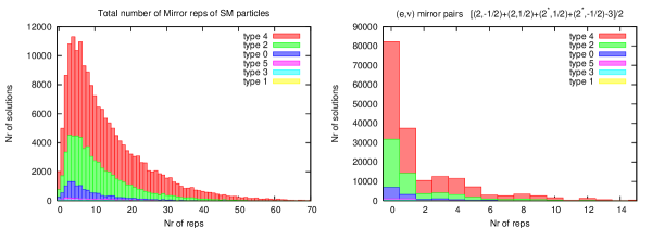
Figure 1: Mirrors

It is interesting to see that the distribution of number of mirrors is sharply peeked at zero mirrors. From the total plot we see that 2018 models have no mirrors at all and that the distribution peeks at 4 mirrors.

The only bifundamentals coming from string states between the standard model branes which should not be chiral are strings stretched between branes a and d. These particles would be leptoquarks. In figure 2 we plot the number of non-chiral leptoquarks.

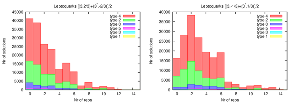
Figure 2: Non-Chiral Leptoquarks

The distribution of leptoquarks with equal sign lepton and baryon number is peaked at zero. This is the only non-chiral ’exotic’ that peaks at zero (apart from individual mirror distributions, as noted above). The distribution of the opposite sign leptoquarks distribution peaks at 2.

Finally one can have massless non-chiral representations coming from strings that have both ends on the same SM brane (or one end on the conjugate brane). These states are symmetric, anti-symmetric or adjoint tensors of the standard model gauge group. The distributions of non-chiral pairs of all these particles peak at a non-zero value, except for the ones where in a majority of the models that particular state does not exist. In 3 we plot the total number of these particles in a model and the distribution of adjoints of $SU(3)$ as an example.

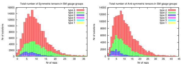
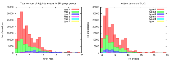
Figure 3: Non-Chiral tensor representations

5.3 Higgs

In supersymmetric extensions of the standard model the Higgs always comes in non-chiral (w.r.t. to $G_{SM}$) pairs so the Higgsinos will not generate an Y-anomaly. In figure 4 we plot the number of Higgsino pairs, which is thus equal to half the number of standard model Higgs doublets in that model.

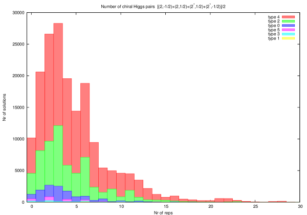
Figure 4: Number of Higgs

As is clear from the picture, the number of Higgs pairs peaks at three. The maximum number of Higgs pairs we found is 56. Note that there also models with no Higgs. These models have an obvious deficiency, although it is conceivable that some (composite-)particle from the hidden sector will play the rôle of the Higgs.

For types based on $U(2)_{\rm b}$ (type 1,3 and 5) there is a possibility for the Higgs of being chiral with respect to $U(2)_{\rm b}$. This chirality was ignored in figure 4, but the chirality distribution is display in LABEL:tbl:nr_sols, as explained above.

5.4 Hidden branes

Our search algorithm was set up to maximize the different standard model spectra, not the hidden brane degrees of freedom. Hence we present in all plots and tables the number of solutions where we identified solutions with different hidden sectors, but which are otherwise equivalent. As explained in section 1.3 we did however construct all solutions containing 0,1 and 2 extra branes for all standard model brane stacks, three extra branes for all stacks with less than 400 candidate hidden CP groups, and four extra branes for less than 100 candidate hidden CP groups. In many other cases we attempted to extract a solution from the tadpole equations without a limit on the number of branes. The latter searches were stopped as soon a one solution was found and are limited by computer time constraints. Therefore they are not systematic. In figure 5 we show the total number of solutions found for each hidden brane multiplicity. This plot is based on a total of 10526078 solutions. These solutions are different only in the sense that their CP multiplicities are distinct. Undoubtedly there are still some equivalences in this set that were not taken into account. The number of solutions with 0,1 and 2 branes is 31215, 148324 and 1170556 respectively.

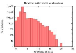
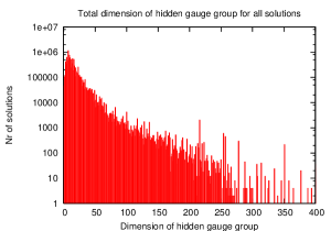
Figure 5: Hidden sector of all solutions

As one can see, the number of solutions grows very fast with the number of hidden branes, but is cut off beyond three branes for the reasons explained above. One can make a plausible guess what the picture might really look like, had we been able to push the search for solutions much further. Most likely, it would continue growing dramatically for quite a while. Since the number of candidate CP groups is typically a few hundred, the distribution necessarily peaks well below that number, but this could easily be around ten or twenty. It is clear that the total number of solutions with distinct standard model plus hidden spectrum can be many orders of magnitude larger than those we found. In figure 5 we plot the total dimension of the total hidden gauge group. The biggest gauge group we encountered has dim 780. The biggest factors we found are $SO(18)$, $Sp(24)$ and $U(18)$.

5.5 Gauge couplings

A remarkable property of the standard model is that its gauge group fits naturally within the gauge group $SU(5)$. This explains two empirical facts: the observed quantization of electric charge, and the observed convergence of the coupling constants at short distances (although with present data, the latter success only survives if the additional assumption of supersymmetry is made). Both of these nice features seem to be lost in the class of models considered here.

Fractional charges are inevitable if there exist additional branes outside the standard model. Strings stretching between the standard model and the hidden branes yield particles (fundamental or QCD bound states) with half-integer electric charge. Although they may be non-chiral (as they are in all models presented here) or even completely absent from the massless spectrum, they exist inevitably as massive open string states. Interestingly, it is not completely straightforward to realize group-theoretical unification in heterotic strings either. In the standard realizations with Kac-Moody level 1 one ether gets $SU(5)$ without a massless Higgs boson to break it, or one gets $SU(3)\times SU(2)\times U(1)$ with additional (though not necessarily massless) fractional charges [16]. These problems can be avoided, for example by considering higher Kac-Moody levels, but it is difficult to argue that charge quantization is a natural property of string theory.

Heterotic $SU(5)$ and $SO(10)$ models do explain the observed coupling constant convergence, but they make a troublesome prediction for the unification scale, which is off by two to three orders of magnitude. It is on this point that open string models have an advantage, simply because there is no such prediction [22]. But there is also no prediction for the unification of the gauge couplings, because they emerge from dilaton couplings of four, a priori unrelated, branes.

In [76] it is argued that a realization of a supersymmetric extension of the standard model with intersecting branes naturally leads to a model where respectively branes $a$ and $d$ and $c$ and $b$ wrap the same cycles. This leads then at the string scale to the following relation between the three standard model coupling constants:

$$\frac{1}{\alpha_{Y}}=\frac{2}{3}\frac{1}{\alpha_{s}}+\frac{1}{\alpha_{w}}.$$ (71)

That would mean that these models do not necessarily have full unification, but they do reproduce a relation which is compatible with the $SU(5)$ relation between the coupling constants.

To do a proper calculation of gauge unification we would have to assume a unification scale and evolve the couplings downward from that scale. Since we are in a rational point of the moduli space, this scale is fixed to a value of order the string scale. The massless spectrum we obtain contains, in general, several non-chiral particles that are presumably artifacts of the rational points. If one assumes that all these particles remain massless until the TeV scale, one should take them into account in the renormalization group flow. More ambitiously, one could work out the masses and the gauge couplings as a function of the moduli near the rational point, and take all of this into account. Here we will only address a simpler question, namely if there is any evidence for relations among the couplings at the string scale. If there is no relation, then clearly one might still get the correct low energy gauge couplings by starting outside the unification point in the space of couplings, and compensate this with exotic matter in the renormalization group flow, but the concept of unification is then anyway lost.

The coupling constants can be computed as follows. Up to a universal factor , they are given by

$$\frac{1}{g_{\rm a}^{2}}=R_{0{\rm a}}e^{\phi}$$ (72)

for CP-groups of orthogonal and symplectic type and

$$\frac{1}{g_{\rm a}^{2}}=(R_{0{\rm a}}+R_{0a^{c}})e^{\phi}=2R_{0{\rm a}}e^{\phi}$$ (73)

for unitary groups, with the conventional normalization $\rm{Tr~{}}T^{a}T^{b}=\frac{1}{2}\delta^{ab}$ for the generators in all three cases. This immediately gives the following expression for the ratio of weak and string couplings:

$${g_{2}^{2}\over g_{3}^{2}}={R_{0{\rm a}}\over\kappa R_{0{\rm b}}}$$ (74)

where $\kappa=1$ for spectra of types 1,3 and 5, and $\kappa=\frac{1}{2}$ for spectra of type 0,2 and 4. The canonically normalized $U(1)$ generator of stack a is $Y_{\rm a}=\frac{1}{\sqrt{6}}\bf{1}$, for stack d it is $Y_{\rm d}=\frac{1}{\sqrt{2}}\bf{1}$, and for stack c it is $Y_{\rm c}=\frac{1}{\sqrt{2}}\bf{1}$ for complex boundaries, and $Y_{\rm c}=\frac{1}{2}\sigma_{3}$ for real ones. The standard model $U(1)$ factor $Y$ is the given by

$${1\over\sqrt{6}}Y_{\rm a}-{1\over\sqrt{2}}Y_{\rm c}-{1\over\sqrt{2}}Y_{\rm d}$$ (75)

for types 0 and 1, and

$${1\over\sqrt{6}}Y_{\rm a}-Y_{\rm c}-{1\over\sqrt{2}}Y_{\rm d}$$ (76)

for types 2,3,4 and 5. This leads to the following expression for the coupling constants

$${1\over g_{Y}^{2}}=\frac{1}{6}{1\over g_{\rm a}^{2}}+\frac{1}{2}{1\over g_{\rm c}^{2}}+\frac{1}{2}{1\over g_{\rm d}^{2}}$$ (77)

for types 0 and 1, and

$${1\over g_{Y}^{2}}=\frac{1}{6}{1\over g_{\rm a}^{2}}+{1\over g_{\rm c}^{2}}+\frac{1}{2}{1\over g_{\rm d}^{2}}$$ (78)

for types 2,3,4 and 5. Hence in both cases the expression for the couplings in terms of reflection coefficients is the same:

$${1\over g_{Y}^{2}}=({1\over 3}R_{0{\rm a}}+R_{0{\rm c}}+R_{0{\rm d}})$$ (79)

The fact that the same expression is obtained is due to the fact that an orthogonal or symplectic c-stack can be viewed as a limit of a unitary one, with the two conjugate branes moved on top of the orientifold plane. From this expression we obtain the following formula for ${\rm{sin}}^{2}\theta_{W}=g_{Y}^{2}/(g_{2}^{2}+g_{Y}^{2})$:

$$\sin^{2}\theta_{W}=\frac{\kappa R_{0{\rm b}}}{\kappa R_{0{\rm b}}+\frac{1}{6}R_{0{\rm a}}+\frac{1}{2}R_{0{\rm c}}+\frac{1}{2}R_{0{\rm d}}}$$ (80)

In figure 6 we plot $\sin^{2}(\theta_{w})$ against the ratio $\alpha_{s}/\alpha_{w}$. In this plot the value for $SU(5)$ unification are also indicated, as well as its renormalization group flow. The solid line denotes the upper limit on $\sin^{2}(\theta_{w})$. Clearly the models we found occupy a substantial part of the allowed region. It is amusing to see that this point falls neatly in the middle of the cloud formed by our models.

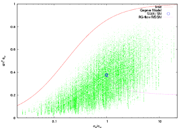
Figure 6: Gauge coupling constants at the string scale

One aspect of the plot that attracts attention is a faint line roughly in the middle of the cloud. It turns out to be described by relation (71). Approximately 10% of the models is on that line. Not surprisingly, these models are characterized by the fact that the reflection coefficients for respectively branes $a$ and $d$ and branes $b$ and $c$ are the same, which is precisely the RCFT equivalent of the condition that [76] used for unification. So although a portion of the models we found has a relation between the coupling constants compatible with $SU(5)$ unification, this is certainly not a generic feature.

5.6 Varying number of chiral families

For a limited set of models we repeated our search for the standard model spectrum with a different number of families, in order to get a feeling what the constraint of having 3 chiral families means. Because more chiral particles implies more intersections one could expect that getting a spectrum with more chiral families is harder. Indeed this tendency is visible in plots 7.

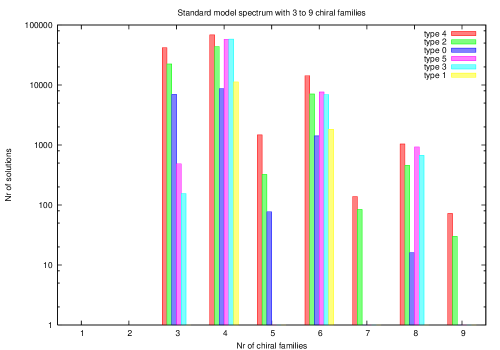
Figure 7: Solutions for varying number of chiral families

Because the number of standard model brane configurations to be analyzed for 1 and 2 families was so big, we performed a search for 1 up to 9 families for 18 models and a search for 3 up to 9 models for a bigger set of 78 models.

But there is more structure. For example odd types (the ones based on $U(2)_{\rm b}$) are much more abundant with even families. If one takes a closer look and distinguishes by subtype, that is the way the $U(2)_{\rm b}$ anomaly cancels, this becomes a bit clearer. Both states coming from $[b,x]$ and $[b^{*},x]$ can contribute to the total chirality of the $SU(2)_{W}$ doublets. They do however contribute oppositely to the $U(2)$ anomaly. This leaves the possibility to cancel the anomaly between the different $U(2)$ chiralities of a doublet. In the even family number models solutions of the subtype where the anomaly cancels fully between the different $U(2)$ chiralities of a given doublet are approximately three orders of magnitude more abundant than subtypes where the anomaly cancels partly between different doublets. Apparently it is easy to have the intersection number of $[b,x]$ equal to that of $[b^{*},x]$. This is also explains why there are so relatively few odd family number solutions with $U(2)_{\rm b}$; For the family number to add up to an odd number, one of the two intersection numbers $[b,x]$ and $[b^{*},x]$ has to be odd and the other even. The easy way of cancelling the anomaly is not a possibility.

Under the assumption that more chiral intersections are harder to get, we can also understand why 4, 2, 3 and 5 are typically less abundant then types 0 and 1. The latter types are based on $U(1)_{\rm c}$ and have all weak singlets coming from their own intersection, with $c$ or $c^{c}$. The former types however, have a real $c$-brane and both lepton singlets (and both quark singlets) come from the same intersection. This means that they have 2 times the number of families less chiral intersections.

A similar effect doesn’t occur if we exchange $U(2)_{\rm b}$ for $Sp(2)_{\rm b}$, because as discussed above, both $U(2)_{\rm b}$ chiralities contribute to one doublet. Hence both types based on $U(2)_{\rm b}$ and $Sp(2)_{\rm b}$ have the same number of chiral $b$-brane intersections.

Also in the other types there is a clear even/odd effect. But if one looks, for odd/even family number separately, at the trend in the number of solutions for a certain type against family number it is to good approximation an exponential drop.

One feature that deserves mentioning is the occurrence of type 1 models with a massive $B-L$ for 1,2 and 4 families, something we didn’t find for three families. These models have as the gauge group that couples to the standard model particles precisely the standard model. That this didn’t occur for three families is probably a matter of statistics. As we have seen type 1 models with three families are already rare, and furthermore from the search for 1,2 and 4 family number models we know that a massive $B-L$ only happens in a few percent of the type 1 solutions.

6 The simplest case

Here we will discuss in some detail one of the simplest cases where a solution was found. It occurs for the tensor product $(1,1,1,1,7,16)$. This has 1944 primaries, 81 of which are simple currents forming a discrete group $\mathbb{Z}_{3}\times\mathbb{Z}_{3}\times\mathbb{Z}_{3}\times\mathbb{Z}_{3}$. Since there are only odd factors, there is just one orientifold choice for each MIPF.

After removing all permutations of the identical factors, this tensor product has 34 simple currents MIPFs. Only one of them has standard-model-like (a,b,c,d) branes. This MIPF is defined by a simple current group that is isomorphic to $\mathbb{Z}_{3}\times\mathbb{Z}_{3}\times\mathbb{Z}_{3}$, and is generated by the three currents $[0,0,0,0,(1,-1,0),(7,3,0),0]$, $[0,0,0,0,(1,-1,0),(7,3,0),0]$ and $[0,0,(1,-1,0),0,0,(7,-5,0),(16,16,0)]$. Out notation is as follows: between the square brackets we indicate the decomposition of the tensor product representation into minimal model representations, with the first entry in each square bracket representing the space-time sector. The minimal model representations are indicated in the usual way as $(l,q,s)$, except for the vacuum, which is denoted as ”0”. Note that only orbit representatives are shown: The minimal model representations are subject to field identification, and the entire tensor representation is actually just one representative of a chiral algebra orbit. Hence other, but equivalent, expressions can be given.

The matrix $X$ yielding the MIPF under consideration is

$$\frac{1}{3}\begin{pmatrix}1&0&1\\ 0&1&1\\ 1&1&1\\ \end{pmatrix}$$

This yields a closed string spectrum corresponding to Hodge numbers $(23,23)$, and a heterotic spectrum with 217 singlets. There are 72 Ishibashi states and hence the same number of boundary states. The total number of sets of (a,b,c,d) stacks is six, all of them of type 3. Three sets saturate the dilaton tadpole condition, whereas the other three do not. We find that for the former all other 17 tadpole conditions are also satisfied, whereas for the latter three there is no possibility of adding branes in order to solve the tadpole conditions. The three sets of boundaries yielding solutions can be described as follows

$$\text{set 1}:\ \ ({\rm a}_{1},{\rm a}_{1}^{c})({\rm b},{\rm b}^{c})({\rm c})({\rm{\rm d}},{\rm d}^{c})$$

$$\text{set 2}:\ \ ({\rm a}_{2},{\rm a}_{2}^{c})({\rm b},{\rm b}^{c})({\rm c})({\rm{\rm d}},{\rm d}^{c})$$

$$\text{set 3}:\ \ ({\rm a}_{3},{\rm a}_{3}^{c})({\rm b},{\rm b}^{c})({\rm c})({\rm{\rm d}},{\rm d}^{c})$$

in other words, the b,c and d branes are always identical, and the complete set of boundaries we need is given by

$${\rm a}_{1}: [0,0,0,0,0,(1,-1,0),(2,2,0)]$$

$${\rm a}_{1}^{c}: [0,0,0,0,0,(1,1,0),(2,-2,0)]$$

$${\rm a}_{2}: [0,0,0,0,0,(1,-1,0),(8,2,0)]_{1}$$

$${\rm a}_{2}^{c}: [0,0,0,0,0,(6,4,0),(8,-8,0)]_{1}$$

$${\rm a}_{3}^{c}: [0,0,0,0,0,(1,-1,0),(8,2,0)]_{2}$$

$${\rm a}_{3}^{c}: [0,0,0,0,0,(6,4,0),(8,-8,0)]_{2}$$

$${\rm b}_{\phantom{1}}: [0,(1,-1,0),(1,-1,0),(1,-1,0),(1,-1,0),(6,-6,0),0]$$

$${\rm b}^{c}: [0,(1,1,0),(1,1,0),(1,1,0),(1,1,0),60,0]$$

$${\rm c}_{\phantom{1}}: [0,0,0,0,(1,1,0),(7,7,0),(16,16,0)]$$

$${\rm d}_{\phantom{1}}: [0,0,0,0,0,(7,7,0),(16,-14,0)]$$

$${\rm d}^{c}: [0,0,0,0,0,(7,-7,0),(16,14,0)]$$

The three sets only differ in the choice of the $U(3)$-brane. The last two choices, ${\rm a}_{2}$ and ${\rm a}_{3}$ and their boundary conjugates, are resolved fixed points of the supercurrent extension of the tensor product., and they differ only in their fixed point degeneracy labels, indicated here as 1 and 2. Not surprisingly, they yield the same spectrum. The spectra of sets 1 and 2 are distinct, and are as follows

$$5(V,V^{*},0,0)_{3}+9(V,0,V,0)_{-3}+$$

$$5(0,V,V,0)_{3}+3(0,V,0,V)_{3}+$$

$$3(0,0,V,V)_{-3}+12(V,V,0,0)_{0}+$$

$$4(0,V,0,V^{*})_{0}+8(Ad,0,0,0)_{0}+$$

$$4(A,0,0,0)_{0}+8(S,0,0,0)_{0}+$$

$$4(0,A,0,0)_{0}+3(0,0,S,0)_{0}+$$

$$4(0,0,0,A)_{0}$$

and

$$3(V,V^{*},0,0)_{3}+9(V,0,V,0)_{-3}+$$

$$5(0,V,V,0)_{3}+3(0,V,0,V)_{3}+$$

$$3(0,0,V,V)_{-3}+4(V,V,0,0)_{0}+$$

$$4(0,V,0,V^{*})_{0}+4(Ad,0,0,0)_{0}+$$

$$4(A,0,0,0)_{0}+6(S,0,0,0)_{0}+$$

$$4(0,A,0,0)_{0}+3(0,0,S,0)_{0}+$$

$$4(0,0,0,A)_{0}$$

The notation is as follows: $V$ denotes a vector, $A$ and anti-symmetric tensor, $S$ a symmetric tensor and $Ad$ and adjoint representation. The $*$ denote complex conjugation, and the last subscript denotes the net chirality of the representation. Our convention is to represent all four-dimensional fermions as left-handed spinors. The precise meaning of, for example, $N\times(V,V^{*},0,0)_{M}$ is then $\frac{1}{2}{(N+M)}(V,V^{*},0,0)+\frac{1}{2}{(N-M)}(V^{*},V,0,0)$. Hence in the first case, we have 3 chiral standard model $SU(3)\times SU(2)\times U(1)$ multiplets $(3,2,\frac{1}{6})$, plus a single mirror pair $(3,2,\frac{1}{6})$+$(3^{*},2,-\frac{1}{6})$. Note that the second factor is actually $U(2)$ instead of $SU(2)$. The additional $U(1)$ is anomalous, and the corresponding gauge boson acquires a mass. The mirrors are non-chiral not just with respect to the standard model group, but with respect to the full group (although this was not a priori required). There is a second set of fully non-chiral mirrors of the same standard model representation in both cases, six in the first and 2 in the second. These differ from the former ones by having opposite $U(1)_{\rm b}$-charges. The tadpole equations satisfied by these two cases are in fact identical.

Since these spectra only differ by the choice of the $a$-branes, the lepton and Higgs sectors are identical. Both have 5 Higgs pairs $(1,2,\frac{1}{2})+(1,2,-\frac{1}{2})$, with the interesting feature that 3 of them are chiral with respect to the $U(2)$ group. Another noteworthy feature is the absence of lepto-quarks.

Finally we present the closed spectrum. The only model-dependent feature concerns the diagonal sector. It turns out that all relevant multiplicities are 1, and that all non-vanishing Klein bottle coefficients are 1. The 23 closed string vector multiplets originate from 21 diagonal fields in the closed string partition function, and two off-diagonal ones. Of the first 21 only the symmetric components survive the Klein bottle projection, and the two off-diagonal ones are reduced to a single field, consisting of a symmetric and an anti-symmetric component. Hence the projected closed string spectrum consists of a supergravity multiplet, one vector multiplet and 22 chiral multiplets originating from $h_{11}$ and another 23 chiral multiplets originating from $h_{21}$.

7 Conclusions

We performed the first semi-systematic search for standard model spectra in open string models. We presented 179520 models that have as their chiral spectrum just the standard model. Most of the models do have non-chiral exotics and/or mirrors, for which we presented the abundances. The number of Higgs was left a free parameter. We found models with as much as 56 Higgses. The distribution peaks at three pairs of Higgs. We also calculated the standard model gauge couplings and found (perhaps not surprisingly) no relation that hinted at unification.

Although we are confident that within the Gepner models we constructed most realizations of the “standard” four stack model, there is much room for improvement and generalization.

More MIPFs of the Gepner models are known than the ones considered here. First of all there are diagonal invariants and their simple current modifications. It turns out that in many cases (but not all) these can be obtained by simple currents, and hence are already included. In other cases more work is needed, see e.g. [77]. Furthermore there are exceptional $SU(2)$ invariants, exceptional invariants of $SU(2)$ tensor products [66], and invariants related to interchanges of fixed points. Unfortunately there is no boundary state formalism available to deal with these cases. There also is no guarantee that we found all orientifolds. Up to now, the orientifold degrees of freedom we use here (Klein bottle currents and crosscap signs) has included everything known by other methods, but most likely this is just a conjecture awaiting a counter example.

There are additional $N=2$ coset CFT´s and presumably even RCFT´s that are not cosets. Indeed, there is a the much larger class of Kazami-Suzuki [78] models. In principle our methods are applicable to these models as well, provided we know the exact spectrum. In cases without field identification fixed points this can be computed straightforwardly, but if there are fixed points the formalism has not been developed yet. Another class that might be accessible with similar methods are the interchange orbifolds of identical minimal or Kazami-Suzuki models [79, 80].

To get an idea how much is still missing, note that we encountered “only” 873 different Hodge number pairs, while for example in [81] already more than 30,000 are presented.

For any accessible RCFT one may consider other brane constructions than the four stack model, for example a construction that would yield $SU(5)$ unification at the string scale, or broken versions of such a model. This would have the obvious advantage of restoring gauge unification. One could also look for Pati-Salam like models, and for models that require a brane recombination mechanism to yield the standard model. As mentioned in the introduction, examples of these types have been constructed already. In principle there is no reason why the standard model could not be realized in such a way, but of course this opens a Pandora’s box of possibilities. The number of solutions would explode even more if we were to allow chiral exotics, a possibility that can never be rigorously ruled out experimentally. But if indeed the quarks and leptons we know today provide misleading information about the true chiral spectrum of nature, then the goal of finding the standard model in string theory is essentially unachievable at present.

The obvious way to control this explosion of candidate standard models is to apply more constraints. There are several criteria that might be used to reject some of the many models on our list, such as absence of a Higgs candidate, the absence of plausible mechanisms to break $Sp(2)_{\rm c}$, or to generate a $B-L$ gauge boson mass. However, it is hard to come up with a criterium that is at the same time very effective and unquestionable.

One could also try to work out the Yukawa coupling of the standard model particles to the Higgs sector. This requires open string three-point couplings, computable in principle in RCFT, but not yet in practice. In cases with more than one supersymmetric Higgs pair, there is the obvious problem of deciding which combination gets a vacuum expectation value. This could be treated as a set of free parameters, and fitted to the observed couplings. Doing that would requires a renormalization group evolution of those couplings, which in its turn requires detailed knowledge of the full (chiral and non-chiral) light spectrum. Then one still faces the problem of the moduli-dependence of the result. To some extent, this may be studied by probing some directions in moduli space with a large number of rational points, as we did for the gauge couplings. However, such an effort is probably premature. Most likely an essential ingredient is missing for the understanding of Yukawa couplings, and that is especially true for neutrino masses.

Fortunately more experimental constraints can be expected in the coming years, especially from the LHC, and also from neutrino and astrophysics experiments. With more experimental input we might come to the conclusion that another type of model should be searched for, and with a different set of constraints. It is to be expected that the class considered here will yield equally rich and abundant results in other cases.

Acknowledgements:
We would like to thank Dieter Lüst for suggesting a check of the results of [76]. We would like to thank Jeff Templon, David Groep, and Davide Salomoni for assistence with running jobs on the NIKHEF computer farm. The work of A.N.S. has been performed as part of the program FP 52 of the Foundation for Fundamental Research of Matter (FOM), and the work of T.P.T.D. and A.N.S. has been performed as part of the program FP 57 of FOM. The work A.N.S. has been partially supported by funding of the Spanish “Ministerio de Ciencia y Tecnología”, Project BFM2002-03610. The work of L.R.H. wass supported in part by the Federal Office for Scientific, Technical and Cultural Affairs through the ”Interuniversity Attraction Poles Programme – Belgian Science Policy” P5/27.

8 Appendix: Boundary and Ishibashi orbits

To compute all annuli using the formalism of [62] it is sufficient to compute all reflection coefficients, and use (21), summing over all Ishibashi labels to compute all annuli $A^{i}_{~{}ab}$. Computationally this scales as $N_{i}(N_{B})^{3}$, where $N_{i}$ is the number of primaries one needs to consider (in our case only the massless ones) and $N_{B}$ the number of boundaries, or equivalently, the number of Ishibashi labels. This sort of computation is analogous to the computation of the fusion coefficients using the Verlinde formula, which, for $N$ primaries, scales as $N^{4}$. In the latter case, such computations can be speeded up drastically if there is a non-trivial simple current group ${\cal G}$. This leads to relations among the matrix elements of the matrix $S$ of the form

$$S_{Ji,j}=e^{2\pi iQ_{J}(j)}S_{ij}\ .$$ (81)

Fusion computations can then be made more efficient for the following three reasons

1. Simple current charge conservation, i.e.
   $N_{abc}=0$ if $Q_{J}(a)\!+Q_{J}(b)\!+Q_{J}(c)\not=0\mod 1$.

2. Simple current relations among fusion entries, $N_{Ka,Jb,Lc}=N_{abc}$ if $JL=K$

3. The summation in the Verlinde formula can be restricted to orbit representatives.

In the absence of fixed points, i.e if all orbit are equally long, this reduces the size of the computation by a factor $|{\cal G}|^{4}$ to $(N_{O})^{4}$, where $N_{O}$ is the number of orbits.

In the present case the quantity of interest is $A^{i}_{~{}ab}$, for a subset of labels $i$. In order to make use of similar results, we have to establish an action of simple currents on the boundary labels $a$ as well as an action on the Ishibashi labels in the internal summation.

First we define a boundary simple current. Consider the oriented annulus

$$A_{ia}^{~{}~{}b}=\sum_{m}{S_{im}\over S_{0m}}R_{ma}R_{mb}^{*}\ ,$$

where for simplicity the boundary and Ishibashi labels $a$ and $m$ implicitly include the degeneracy label. The labels $i$ are primaries of the bulk CFT, and we can consider the case that $i$ is a simple current, $J$. Then one can show that for every $a$ there is precisely one $b$ such that $A_{Ja}^{~{}~{}~{}}b=1$, and that for all other $b$ this quantity vanishes. The proof goes as follows.

$$A_{Ja}^{~{}~{}~{}b}=\sum_{m}{S_{Jm}\over S_{0m}}R_{ma}R_{mb}^{*}=\sum_{m}e^{2\pi iQ_{J}(m)}R_{ma}R_{mb}^{*}$$

For each $a$, the vectors $R_{ma}$ have norm 1. Hence this sum can at most be 1, and it is equal to 1 if and only if

$$R_{mb}=e^{2\pi iQ_{J}(m)}R_{ma}$$ (82)

Since the boundaries are independent, there can be at most one boundary $b$ that satisfies this. and since the set is complete, there must be precisely one (note that the matrix $A_{J}$ has to satisfy the completeness condition $A_{J}A_{J^{c}}={\bf 1}$ and hence cannot have an entire row that is zero). Hence it makes sense to define $J\cdot a\equiv b$ as the action of $J$ on $a$. Using (82) one can easily show that

$$A_{i,J\cdot a}^{~{}~{}J\cdot b}=A_{ia}^{~{}~{}b}\ .$$

This establishes the second of the three properties listed above, with $K=1$. Since the label $i$ is restricted to massless fields a further generalization analogous to $K\not=1$ is not really useful, since the simple current action on $i$ does not preserve its conformal weight.

A simple current $J$ may yield a trivial action on all boundaries. It is easy to show that $J\cdot(K\cdot a)=(JK\cdot a)=K\cdot(J\cdot a)$, where $JK$ denotes the fusion product of the CFT. Therefore if $J$ and $K$ both fix all boundaries, so does $JK$, and hence the set of simple currents that fix all boundaries is a subgroup ${\cal G}_{X}$ of ${\cal G}$. The boundary simple current group is defined as the discrete group ${\cal G}/{\cal G}_{X}$. The elements of that group have distinct actions on at least one of the boundaries.

In all cases covered by the simple current formalism of [62] there is a special boundary originating from the CFT vacuum state, $a=0$. One might conjecture a natural correspondence between the elements of the boundary simple current group and the set of boundaries obtained by the action of ${\cal G}$ on the boundary 0. However, it turns out that this is not a one-to-one correspondence: it may happen that $J\cdot 0=0$, but $J\cdot a\not=a$ for some other $a$. Hence the boundary simple current group may be larger than the set of “simple current boundaries”.

Relation (82) is the analog of (81) for the action on the boundary label. An action on the Ishibashi label can be derived directly from (26) and (28):

$$R_{(Im,J)[a,\psi_{a}]}=F_{m}(I,J)e^{2\pi iQ_{I}(a)}R_{(m,J)[a,\psi_{a}]}\ ,$$ (83)

if the set of degeneracy labels $J$ for $m$ and $Lm$ are the same. This is the case if and only if $L$ is local with respect to the simple current group ${\cal H}$ that defines the MIPF. The subgroup of ${\cal G}$ with that property will be called the Ishibashi simple current group. The simple current twist $F_{m}(I,J)$ is a sign in all known cases, and this implies that its occurrence here is irrelevant, since we are free to change all boundary and crosscap coefficients simultaneously by signs: $R_{ma}\to\epsilon_{m}R_{ma},U_{m}\to\epsilon_{m}U_{m}$. This allows us to redefine the boundary coefficients on each Ishibashi orbit in such a way that for the orbit representatives, $m_{0}$, we get simply

$$R_{(Im_{0},J)[a,\psi_{a}]}=e^{2\pi iQ_{I}(a)}R_{(m_{0},J)[a,\psi_{a}]}\ ,$$ (84)

Note that the crosscap coefficients $U_{m,J}$ vanish if $J\not=0$, so these sign changes are irrelevant for crosscaps.

Now consider the first simplification listed above, charge conservation. The annulus amplitude $A^{i}_{~{}ab}$ can be expressed in terms of the fixed point fusion coefficients [73]

$$(N^{J})^{j}_{ab}=\sum_{m}{S_{jm}^{*}\over S_{0m}}S^{J}_{ma}S^{J^{c}}_{mb}\ .$$

as a linear combination of the form

$$\sum_{L\in{\cal H}}\sum_{J\in cH}\phi(L,J,a,b)(N^{J})^{KLi}_{ab}\ ,$$

Here $\phi(L,J,a,b)$ are complex coefficients and $K$ is the Klein bottle current. Using 28 and the property $F_{a}(K,N)F_{a}(K,M)=F_{a}(K,NM)$ it follows that $(N^{J})^{j}_{ab}=0$ unless $Q_{M}(a)+Q_{M}(b)=Q_{M}(j)\mod 1$ for all simple currents $M$. For the annulus this implies that $A^{i}_{~{}ab}=0$ unless there is an $L\in{\cal H}$ so that $Q_{M}(a)+Q_{M}(b)\not=Q_{M}(i)+Q_{M}(K)+Q_{M}(L)\mod 1$.

Finally consider the third simplification. The sum over $m$ can be reduced to a sum over Ishibashi orbit representatives provided that charge conservation is satisfied, i.e $Q_{I}(a)+Q_{I}(b)\not=Q_{I}(i)+Q_{I}(K)+Q_{I}(L)\mod 1$, for all $L\in{\cal H}$. Since Ishibashi currents $I$ are always local with respect to ${\cal H}$, this condition is always satisfied.

9 Bibliography

10 Tables

Table 1: List of standard model representations that can appear, and their labelling.

nr.	$U(3)_{\rm a}$	$U(2)_{\rm b}$	$Sp(2)_{\rm b}$	$U(1)_{\rm c}$	$SO(2)_{\rm c}$	$U(1)_{\rm d}$	massless particle
					$Sp(2)_{\rm c}$
1	$V$	$V$	$\left.\right\rmoustache$ $V$	0		0	$(u,d)$
2	$V$	$V^{*}$	$\left.\right\lmoustache$	0		0	$(u,d)$
3	$V^{*}$	0		$V$	$\left.\right\rmoustache$ $V$	0	$u^{c}$
4	$V^{*}$	0		$V^{*}$	$\left.\right\lmoustache$	0	$d^{c}$
5	0	$V$	$\left.\right\rmoustache$ $V$	0		$V$	$(\nu,e^{-})$
6	0	$V^{*}$	$\left.\right\lmoustache$	0		$V$	$(\nu,e^{-})$
7	0	0		$V$	$\left.\right\rmoustache$ $V$	$V^{*}$	$\nu^{c}$
8	0	0		$V^{*}$	$\left.\right\lmoustache$	$V^{*}$	$e^{+}$
9	0	$V$		$V$		0	$H_{1}$
10	0	$V$		$V^{*}$		0	$H_{2}$
11	$V$	0		0		$V$	$(3,1,-\frac{1}{3})_{1,1}$
12	$V$	0		0		$V^{*}$	$(3,1,\frac{2}{3})_{1,-1}$
13	Adj	0		0		0	$(8,1,0)_{0,0}+(1,1,0)_{0,0}$
14	A	0		0		0	$(3^{*},1,\frac{1}{3})_{2,0}$
15	S	0		0		0	$(6,1,\frac{1}{3})_{2,0}$
16	0	Adj	—	0		0	$(1,3,0)_{0,0}+(1,1,0)_{0,0}$
17	0	A		0		0	$(1,1,0)_{0,0}$
18	0	S		0		0	$(1,3,0)_{0,0}$
19	0	0		Adj	—	0	$(1,1,0)_{0,0}$
20	0	0		—	A	0	$(1,1,-1)_{0,0}$
21	0	0		S		0	$(1,1,-1)_{0,0}$
22	0	0		0		Adj	$(1,1,0)_{0,0}$
23	0	0		0		A	—
24	0	0		0		S	$(1,1,-1)_{0,2}$
25	$V$	0		0		0	$(3,1,\frac{1}{6})_{1,0}$
26	0	$V$		0		0	$(1,2,0)_{0,0}$
27	0	0		$V$		0	$(1,1,-\frac{1}{2})_{0,0}$
28	0	0		0		$V$	$(1,1,-\frac{1}{2})_{0,1}$
29	0	0		0		$0$	$(1,1,0)_{0,0}$

Table 2: Summary results for all Gepner Models

nr.	Tensor	Prim	S.C.	MIPF	Intersect.	Sol.	SM spectra
1	(1,5,41,1804)	28539	1	1,0,0	0	0	0
2	(1,5,42,922)	29772	2	2,-,-	-	-	-
3	(1,5,43,628)	31482	3	2,-,-	-	-	-
4	(1,5,44,481)	9399	1	1,0,0	0	0	0
5	(1,5,46,334) $\dagger$	35442	6	4,1,0	12	0	0
6	(1,5,47,292) $\dagger$	37800	7	2(1),1,0	1128	0	0
7	(1,5,49,236)	4575	1	1,0,0	0	0	0
8	(1,5,52,187)	12690	3	2(1),1,0	144	0	0
9	(1,5,54,166) $\dagger$	48258	14	4,1,0	54	0	0
10	(1,5,58,138)	6156	2	2,0,0	0	0	0
11	(1,5,61,124)	64449	21	4(2),3,0	81044	0	0
12	(1,5,68,103)	20748	7	2(1),1,0	234	0	0
13	(1,5,76,89)	2835	1	1,0,0	0	0	0
14	(1,5,82,82) $\dagger$	108612	42	8(1),3,0	1744	0	0
15	(1,6,23,598)	12600	2	2,0,0	0	0	0
16	(1,6,24,310) $\dagger$	13650	4	6(1),1,0	18260	0	0
17	(1,6,25,214)	14742	6	4(2),2,0	212000	0	0
18	(1,6,26,166)	15876	8	10(7),8,0	4939262	0	0
19	(1,6,28,118)	18270	12	12(9),10,2	1289765	217	67
20	(1,6,30,94)	20664	16	14(12),12,1	2912087	297	221
21	(1,6,31,86)	2464	2	2,0,0	0	0	0
22	(1,6,34,70)	26460	24	20(16),18,4	1539069	2466	1587
23	(1,6,38,58)	8260	8	10(7),8,1	435815	36	18
24	(1,6,40,54)	4018	4	6(3),3,0	87494	0	0
25	(1,6,46,46)	46536	48	28(24),26,5	3687098	67723	16490
26	(1,7,17,340)	9396	3	2,0,0	0	0	0
27	(1,7,18,178)	10224	6	4(1),1,0	29672	0	0
28	(1,7,19,124)	11880	9	6(2),4,0	2513	0	0
29	(1,7,20,97)	4116	3	2,0,0	0	0	0
30	(1,7,22,70)	14760	18	12(6),8,0	38210	0	0
31	(1,7,25,52)	21060	27	10(2),7,0	7523	0	0
32	(1,7,28,43)	7128	9	6,2,0	19	0	0
33	(1,7,34,34)	33264	54	16(8),10,2	62992	70	13
34	(1,8,14,238)	8082	4	6(3),3,1	3447270	16	16
35	(1,8,16,88)	10218	12	12(7),7,0	70962	0	0
36	(1,8,18,58)	12690	20	12(7),9,1	240804	4	2
37	(1,8,22,38)	2034	4	6(1),1,0	2888	0	0
38	(1,8,28,28)	28410	60	20(8),14,2	152706	1288	188
39	(1,9,12,229)	2875	1	1,0,0	0	0	0
40	(1,9,13,108)	1015	1	1,0,0	0	0	0
41	(1,9,20,31)	6160	11	2,0,0	0	0	0
42	(1,10,11,154)	7704	6	4,1,0	372	0	0
43	(1,10,12,82)	8970	12	12(4),9,0	277382	0	0
44	(1,10,13,58)	10332	18	12(4),9,0	19649	0	0
45	(1,10,14,46)	11748	24	20(12),17,3	328229	7389	3687
46	(1,10,16,34)	14994	36	36(18),29,5	198765	503	173
47	(1,10,18,28)	4698	12	12(3),6,2	19344	32	14
48	(1,10,19,26)	2280	6	4,0,0	0	0	0
49	(1,10,22,22)	26532	72	50(20),39,10	499730	15055	2780
50	(1,11,11,76)	9828	13	2,1,0	96	0	0
51	(1,12,12,40)	12138	28	10(2),8,1	22942	8	2
52	(1,12,13,33)	595	1	1,0,0	0	0	0
53	(1,12,19,19)	10500	21	4,0,0	0	0	0
54	(1,13,13,28)	19845	45	10,5,0	1854	0	0
55	(1,13,18,18)	3220	10	4,1,0	20	0	0
56	(1,14,14,22)	5336	16	14(1),10,2	17112	63	23
57	(1,16,16,16)	33210	108	26(5),17,5	125476	9204	494
58	(2,3,19,418)	6320	2	2,0,0	0	0	0
59	(2,3,20,218)	6972	4	6(4),4,0	315210	0	0
60	(2,3,22,118)	8232	8	5(4),4,1	180431	6	4
61	(2,3,23,98)	9120	10	4(1),1,0	1204	0	0
62	(2,3,26,68)	3036	4	6(4),4,0	18416	0	0
63	(2,3,28,58)	13340	20	12(8),9,4	142742	482	176
64	(2,3,34,43)	1232	2	2,0,0	0	0	0
65	(2,3,38,38)	22920	40	10(8),9,2	151792	1044	216
66	(2,4,11,154)	3540	4	6(4),4,0	2304160	0	0
67	(2,4,12,82)	4160	8	30(26),26,12	5133558	598	294
68	(2,4,13,58)	4830	12	12(7),9,1	468648	146	69
69	(2,4,14,46)	5340	16	27(24),25,13	1918601	17411	5607
70	(2,4,16,34)	7140	24	60(48),54,23	3700006	218598	45055
71	(2,4,18,28)	2320	8	30(23),25,15	745644	801	360
72	(2,4,19,26)	1100	4	6(2),3,0	23872	0	0
73	(2,4,22,22)	12060	48	54(39),51,25	3403934	423560	43532
74	(2,5,8,138)	2862	4	6(3),4,0	191424	0	0
75	(2,5,10,40)	1230	4	6(1),3,0	5502	0	0
76	(2,5,12,26)	6006	28	12,7,3	34744	2426	431
77	(2,6,7,70)	3024	8	5(1),3,0	28234	0	0
78	(2,6,8,38)	3780	16	27(18),22,7	323662	6313	1368
79	(2,6,10,22)	5544	32	59(20),53,27	361546	18964	3624
80	(2,6,14,14)	9744	64	87(20),71,30	758636	62856	5424
81	(2,7,7,34)	4032	18	6,0,0	0	0	0
82	(2,7,10,16)	2040	12	12,6,1	10504	4	1
83	(2,8,8,18)	6480	40	44(3),32,16	1019592	222006	17311
84	(2,8,10,13)	630	4	6,3,0	1320	0	0
85	(2,10,10,10)	12000	96	92(7),71,34	850844	137472	9878
86	(3,3,9,108)	2900	5	2,0,0	0	0	0
87	(3,3,10,58)	3280	10	4,1,0	124	0	0
88	(3,3,12,33)	1700	5	2,0,0	0	0	0
89	(3,3,13,28)	6300	25	6,2,0	118	0	0
90	(3,3,18,18)	9200	50	12,4,0	1492	0	0
91	(3,4,6,118)	2100	4	6(3),3,0	176520	0	0
92	(3,4,7,43)	1584	3	2,0,0	0	0	0
93	(3,4,8,28)	3280	20	12(1),7,0	3348	0	0
94	(3,4,10,18)	540	4	6,0,0	0	0	0
95	(3,4,13,13)	4410	15	4,0,0	0	0	0
96	(3,5,5,68)	2394	7	2,0,0	0	0	0
97	(3,6,6,18)	1064	8	10,1,0	88	0	0
98	(3,8,8,8)	9200	100	18,11,2	5406	96	4
99	(4,4,5,40)	2322	12	10,6,0	56000	0	0
100	(4,4,6,22)	3150	24	44(9),33,15	465222	51448	8737
101	(4,4,7,16)	3888	36	26(1),17,6	93764	2590	59
102	(4,4,8,13)	1218	12	10(2),7,0	3682	0	0
103	(4,4,10,10)	7200	72	110(3),74,15	999730	277752	9983
104	(4,5,5,19)	1890	7	2,0,0	0	0	0
105	(4,6,6,10)	1540	16	54,22,3	6874	64	6
106	(4,7,7,7)	5184	27	6,0,0	0	0	0
107	(5,5,5,12)	6615	49	5,0,0	0	0	0
108	(6,6,6,6)	9632	128	76,44,10	174232	70864	1310
109	(1,1,2,11,154)	2124	6	4,0,0	0	0	0
110	(1,1,2,12,82)	2496	12	12,0,0	0	0	0
111	(1,1,2,13,58)	2898	18	10,0,0	0	0	0
112	(1,1,2,14,46)	3204	24	10,2,0	788	0	0
113	(1,1,2,16,34)	4284	36	30,8,0	260	0	0
114	(1,1,2,18,28)	1392	12	12,0,0	0	0	0
115	(1,1,2,19,26)	660	6	4,0,0	0	0	0
116	(1,1,2,22,22)	7236	72	26,7,0	3864	0	0
117	(1,1,3,6,118)	1260	6	4,0,0	0	0	0
118	(1,1,3,7,43)	1584	9	5,0,0	0	0	0
119	(1,1,3,8,28)	2010	30	8,1,0	2	0	0
120	(1,1,3,10,18)	324	6	4,0,0	0	0	0
121	(1,1,3,13,13)	4410	45	10,1,0	54	0	0
122	(1,1,4,5,40)	1431	18	10,0,0	0	0	0
123	(1,1,4,6,22)	1890	36	30,0,0	0	0	0
124	(1,1,4,7,16)	2484	54	40,1,0	2	0	0
125	(1,1,4,8,13)	819	18	10,0,0	0	0	0
126	(1,1,4,10,10)	4320	108	96,6,0	652	0	0
127	(1,1,5,5,19)	1890	21	4,0,0	0	0	0
128	(1,1,6,6,10)	924	24	20,1,0	16	0	0
129	(1,1,7,7,7)	5184	81	19,2,0	8	0	0
130	(1,2,2,5,40)	492	4	6,0,0	0	0	0
131	(1,2,2,6,22)	1512	32	31,7,0	3434	0	0
132	(1,2,2,7,16)	816	12	12,0,0	0	0	0
133	(1,2,2,8,13)	252	4	6,0,0	0	0	0
134	(1,2,2,10,10)	3288	96	120,22,1	7566	72	2
135	(1,2,3,3,58)	920	10	4,0,0	0	0	0
136	(1,2,3,4,18)	160	4	6,0,0	0	0	0
137	(1,2,4,4,10)	2250	72	118,19,4	10920	730	99
138	(1,2,4,6,6)	420	16	27,0,0	0	0	0
139	(1,3,3,3,13)	1400	25	4,0,0	0	0	0
140	(1,3,3,4,8)	260	10	4,0,0	0	0	0
141	(1,4,4,4,4)	4266	216	112,11,2	5552	172	6
142	(2,2,2,3,18)	1040	32	27,2,0	1168	0	0
143	(2,2,2,4,10)	1520	64	230,60,7	48876	4832	92
144	(2,2,2,6,6)	3024	128	305,101,6	111080	10304	95
145	(2,2,3,3,8)	720	20	12,0,0	0	0	0
146	(2,2,4,4,4)	1500	48	180,5,0	4640	0	0
147	(3,3,3,3,3)	4000	125	8,0,0	0	0	0
148	(1,1,1,1,5,40)	972	27	8,0,0	0	0	0
149	(1,1,1,1,6,22)	1134	54	16,0,0	0	0	0
150	(1,1,1,1,7,16)	1944	81	34,1,1	6	3	2
151	(1,1,1,1,8,13)	756	27	8,0,0	0	0	0
152	(1,1,1,1,10,10)	2592	162	58,0,0	0	0	0
153	(1,1,1,2,3,18)	96	6	4,0,0	0	0	0
154	(1,1,1,2,4,10)	1350	108	72,0,0	0	0	0
155	(1,1,1,2,6,6)	252	24	10,0,0	0	0	0
156	(1,1,1,3,3,8)	240	15	4,0,0	0	0	0
157	(1,1,1,4,4,4)	2673	324	142,0,0	0	0	0
158	(1,1,2,2,2,10)	912	96	52,0,0	0	0	0
159	(1,1,2,2,4,4)	900	72	110,0,0	0	0	0
160	(1,2,2,2,2,4)	440	64	138,0,0	0	0	0
161	(2,2,2,2,2,2)	2944	512	1031,10,0	448	0	0
162	(1,1,1,1,1,2,10)	810	162	34,0,0	0	0	0
163	(1,1,1,1,1,4,4)	1944	486	156,0,0	0	0	0
164	(1,1,1,1,2,2,4)	540	108	48,0,0	0	0	0
165	(1,1,1,2,2,2,2)	264	96	46,0,0	0	0	0
166	(1,1,1,1,1,1,1,4)	2187	729	124,0,0	0	0	0
167	(1,1,1,1,1,1,2,2)	324	162	24,0,0	0	0	0
168	(1,1,1,1,1,1,1,1,1)	2187	2187	152,0,0	0	0

Table 3: All MIPFs with solutions

Tensor	$(h_{11},h_{21},S)$	Boundaries	Nr.	Types
(1,6,28,118)	(24,84,429)	2400	6	(6,0,0,0,50,0,0)
	(75,75,565)	6090	2	(2,0,0,2,15,0,0)
(1,6,30,94)	(24,84,425)	1980	6	(6,0,0,0,221,0,0)
(1,6,34,70)	(29,125,557)	3312	10	(10,0,3,2,0,0,0)
	(14,98,451)	1656	9	(9,0,0,0,1557,0,0)
	(43,91,509)	4464	2	(2,0,0,2,11,0,0)
	(29,53,353)	3420	11	(11,0,0,0,6,0,0)
(1,6,38,58)	(29,53,351)	1520	6	(6,0,0,0,18,0,0)
(1,6,46,46)	(19,163,649)	2968	12	(12,0,87,0,11,0,0)
	(9,129,525)	1484	10	(10,0,0,0,16294,0,0)
	(27,123,569)	3944	2	(2,0,4,20,37,0,0)
	(19,67,377)	2968	13	(13,0,6,1,29,0,0)
	(59,59,449)	7888	4	(4,0,0,0,1,0,0)
(1,7,34,34)	(23,95,437)	2136	10	(10,0,0,2,0,0,0)
	(29,77,457)	3696	2	(2,0,7,0,4,0,0)
(1,8,14,238)	(53,53,443)	3252	4	(4,0,0,0,16,0,0)
(1,8,18,58)	(38,62,377)	2538	2	(2,0,0,0,2,0,0)
(1,8,28,28)	(17,95,419)	1894	2	(2,0,110,20,54,0,0)
	(29,29,251)	2316	12	(12,0,4,0,0,0,0)
(1,10,14,46)	(8,68,315)	728	8	(8,0,0,0,3447,0,0)
	(17,41,259)	1540	11	(11,0,123,0,92,0,0)
	(35,59,369)	2000	2	(2,0,0,16,6,0,0)
(1,10,16,34)	(13,97,405)	1088	20	(20,0,8,0,16,0,0)
	(29,65,355)	1666	22	(22,0,20,42,44,10,0)
	(20,32,241)	1920	25	(25,0,6,0,0,0,0)
	(20,32,249)	1920	29	(29,0,9,0,12,0,0)
	(38,38,311)	2544	7	(7,0,0,6,0,0,0)
(1,10,18,28)	(10,46,253)	576	6	(6,0,0,0,12,0,0)
	(23,59,343)	1044	1	(1,0,0,0,2,0,0)
(1,10,22,22)	(7,127,467)	1088	20	(20,0,1,0,4,0,0)
	(17,89,387)	1504	22	(22,0,139,153,130,0,0)
	(7,55,263)	1148	19	(19,0,1227,0,886,0,0)
	(19,67,323)	1804	34	(34,0,0,3,0,0,0)
	(19,67,343)	1876	35	(35,0,0,39,0,0,0)
	(22,58,321)	2256	30	(30,0,0,2,0,0,0)
	(13,37,243)	1632	29	(29,0,8,0,14,0,0)
	(25,49,303)	2256	44	(44,0,0,22,0,0,0)
	(27,51,319)	2256	31	(31,0,31,20,3,0,0)
	(41,41,323)	2948	36	(36,0,0,6,2,0,0)
(1,12,12,40)	(25,85,423)	948	7	(7,0,1,0,1,0,0)
(1,14,14,22)	(23,23,225)	952	9	(9,0,13,0,8,0,0)
	(31,31,273)	1352	13	(13,0,0,2,0,0,0)
(1,16,16,16)	(11,101,401)	1230	12	(12,0,219,0,35,0,15)
	(16,64,325)	2196	13	(13,0,2,2,0,0,0)
	(8,44,227)	1512	14	(14,0,88,0,88,0,0)
	(21,57,301)	2196	16	(16,0,0,40,0,0,0)
	(20,32,243)	1512	10	(10,0,5,0,0,0,0)
(2,3,22,118)	(41,77,463)	2160	4	(4,0,0,0,4,0,0)
(2,3,28,58)	(17,101,463)	1408	6	(6,0,0,0,80,0,0)
	(17,101,463)	1472	8	(8,0,0,0,86,0,0)
	(39,87,475)	2552	1	(1,0,0,0,1,7,0)
	(39,87,475)	2668	2	(2,0,0,0,2,0,0)
(2,3,38,38)	(11,131,533)	1200	7	(7,0,0,0,215,0,0)
	(23,71,389)	2616	8	(8,0,0,1,0,0,0)
(2,4,12,82)	(58,34,371)	2480	12	(12,0,0,0,4,0,0)
	(33,39,325)	1438	28	(28,0,9,0,71,0,0)
	(33,39,325)	1460	11	(11,0,8,0,6,0,0)
	(39,33,325)	1678	27	(27,0,16,0,32,0,0)
	(39,33,325)	1724	15	(15,0,2,0,4,0,0)
	(42,48,357)	1798	29	(29,0,0,0,19,0,0)
	(42,48,357)	1856	9	(9,0,0,0,12,0,0)
	(48,42,357)	2048	19	(19,0,5,0,1,0,1)
	(48,42,357)	2110	4	(4,0,17,0,53,0,1)
	(51,57,447)	2180	13	(13,0,0,0,12,0,17)
	(51,57,447)	2230	6	(6,0,0,0,2,0,0)
	(45,45,350)	2048	8	(8,0,0,0,2,0,0)
(2,4,13,58)	(37,61,413)	1540	1	(1,0,0,0,5,64,0)
(2,4,14,46)	(19,67,339)	864	24	(24,0,0,0,13,0,0)
	(20,56,308)	1152	25	(25,0,173,0,359,0,0)
	(21,57,321)	1152	23	(23,0,0,0,841,0,0)
	(26,62,343)	1440	18	(18,0,21,0,165,4,0)
	(29,65,407)	1440	1	(1,0,24,0,26,24,0)
	(56,20,308)	2640	21	(21,0,0,0,9,0,0)
	(62,26,343)	2796	7	(7,0,1,0,0,0,0)
	(20,44,299)	864	26	(26,0,793,0,1151,0,0)
	(34,58,367)	1728	16	(16,0,6,0,116,0,8)
	(25,37,287)	1152	8	(8,0,318,0,887,0,0)
	(28,40,309)	1440	10	(10,0,6,0,266,0,3)
	(35,47,329)	1440	15	(15,0,3,5,11,0,0)
	(37,25,287)	1896	19	(19,0,3,0,1,0,0)
(2,4,16,34)	(16,100,440)	1000	12	(12,0,0,0,817,0,0)
	(13,73,339)	800	38	(38,0,0,0,19,0,0)
	(13,73,339)	820	44	(44,0,1,0,182,0,0)
	(15,69,339)	962	43	(43,0,28,0,1999,0,0)
	(15,69,339)	1036	11	(11,0,15,0,2086,0,0)
	(21,75,421)	1180	47	(47,0,84,0,861,76,0)
	(21,75,421)	1250	19	(19,0,0,0,184,50,0)
	(12,54,297)	770	41	(41,0,2964,0,4549,0,0)
	(12,54,297)	796	45	(45,0,1248,0,1808,0,0)
	(24,66,353)	1360	15	(15,0,26,0,209,352,24)
	(24,66,353)	1394	20	(20,0,17,0,70,6,0)
	(20,56,306)	1040	36	(36,0,1768,0,2253,0,0)
	(20,56,306)	1120	10	(10,0,504,0,876,0,0)
	(26,62,339)	1144	48	(48,0,80,18,412,68,0)
	(26,62,339)	1232	17	(17,0,4,0,261,14,0)
	(15,45,285)	914	42	(42,0,5345,0,7519,0,0)
	(15,45,285)	976	13	(13,0,1281,0,1855,0,0)
	(23,53,307)	1120	49	(49,0,115,10,266,4,2)
	(23,53,307)	1202	18	(18,0,274,2,803,0,1)
	(22,46,309)	1300	46	(46,0,112,10,511,24,0)
	(22,46,309)	1400	16	(16,0,455,0,931,0,39)
	(31,55,330)	1768	14	(14,0,0,14,0,0,0)
	(31,55,330)	1904	1	(1,0,12,2,23,0,0)
(2,4,18,28)	(26,44,293)	854	27	(27,0,0,0,7,0,0)
	(26,44,293)	976	9	(9,0,0,0,15,0,0)
	(44,26,293)	1024	11	(11,0,8,0,16,0,0)
	(44,26,293)	1166	4	(4,0,3,0,8,0,0)
	(25,37,279)	736	18	(18,0,0,0,12,0,0)
	(24,30,261)	686	28	(28,0,34,0,72,0,0)
	(24,30,261)	724	19	(19,0,31,0,27,0,0)
	(30,24,261)	830	29	(29,0,33,0,44,0,0)
	(30,24,261)	940	15	(15,0,1,0,4,0,0)
	(36,42,327)	1060	21	(21,0,0,0,1,0,0)
	(42,36,327)	1276	17	(17,0,0,0,0,0,1)
	(31,31,270)	896	22	(22,0,0,0,0,0,0)
	(31,31,270)	1024	8	(8,0,2,0,8,0,0)
	(39,39,313)	1036	10	(10,0,0,0,6,0,0)
	(39,39,313)	1184	1	(1,0,0,0,22,0,0)
(2,4,22,22)	(11,131,536)	864	12	(12,0,0,0,1292,0,0)
	(7,103,399)	648	43	(43,0,0,0,71,0,0)
	(14,98,501)	1080	1	(1,38,255,154,1123,158,0)
	(9,81,344)	864	44	(44,0,1113,0,1977,0,0)
	(10,82,361)	864	42	(42,0,0,0,404,0,0)
	(13,85,367)	1080	22	(22,0,169,0,1011,168,0)
	(16,88,393)	1296	20	(20,0,88,68,582,0,61)
	(8,68,329)	648	45	(45,0,5089,0,7025,0,0)
	(14,74,341)	1080	18	(18,0,497,154,1704,0,0)
	(10,58,309)	864	11	(11,0,3162,0,7156,0,0)
	(13,61,335)	1080	13	(13,16,2235,231,2695,81,152)
	(21,69,344)	1728	16	(16,0,147,150,147,0,0)
	(20,56,313)	1788	48	(48,0,138,0,85,0,0)
	(16,40,261)	1416	46	(46,0,120,0,251,0,3)
	(19,43,279)	1476	49	(49,0,274,0,173,0,1)
	(28,52,341)	2160	2	(2,0,0,5,22,56,0)
	(52,28,341)	3888	35	(35,0,0,0,2,0,0)
	(20,32,261)	1668	17	(17,0,383,1,319,1,0)
	(32,44,313)	2412	30	(30,0,0,1,8,0,0)
	(23,23,247)	1356	21	(21,0,0,0,4,0,0)
	(31,31,268)	1968	47	(47,0,43,0,73,0,0)
	(31,31,279)	2460	19	(19,0,0,0,1,4,0)
	(32,32,273)	2040	28	(28,0,27,0,65,0,0)
	(32,32,273)	2592	50	(50,0,1,0,0,0,0)
	(39,39,311)	2100	31	(31,0,0,0,8,0,3)
(2,5,12,26)	(8,80,341)	528	8	(8,0,0,0,32,0,0)
	(23,59,327)	780	1	(1,0,60,0,252,82,0)
	(23,59,327)	858	2	(2,0,0,0,5,0,0)
(2,6,8,38)	(14,50,289)	720	9	(9,0,0,0,530,0,0)
	(21,57,333)	1080	15	(15,0,26,0,14,0,0)
	(26,50,313)	1080	12	(12,0,35,0,33,0,0)
	(28,52,331)	1200	16	(16,0,1,0,74,0,18)
	(22,34,265)	720	25	(25,0,0,0,447,0,0)
	(25,37,271)	1080	1	(1,0,47,0,42,0,0)
	(33,33,275)	1440	13	(13,0,0,0,7,0,0)
(2,6,10,22)	(14,62,299)	864	56	(56,0,150,0,120,0,0)
	(15,63,307)	864	15	(15,0,26,0,34,0,0)
	(16,64,331)	864	58	(58,0,3,0,325,0,0)
	(10,46,253)	432	13	(13,0,0,0,1774,0,0)
	(16,40,249)	864	22	(22,0,76,0,297,0,6)
	(19,43,255)	864	53	(53,0,26,0,36,0,0)
	(22,46,275)	864	20	(20,0,0,0,61,0,0)
	(22,46,319)	1152	38	(38,0,0,0,8,0,0)
	(13,25,215)	864	55	(55,0,0,0,2,0,0)
	(15,27,239)	864	21	(21,0,20,0,18,0,0)
	(17,29,223)	1008	30	(30,0,5,0,0,0,0)
	(18,30,223)	1080	52	(52,0,1,0,7,0,0)
	(20,32,241)	1080	54	(54,0,5,0,59,0,0)
	(20,32,261)	1008	29	(29,0,30,0,60,0,0)
	(22,34,253)	1152	32	(32,0,10,0,55,0,0)
	(26,38,283)	1080	18	(18,0,1,0,2,0,0)
	(29,17,223)	1152	39	(39,0,0,0,11,0,0)
	(32,20,241)	1512	16	(16,0,1,0,5,0,0)
	(32,20,261)	1440	4	(4,0,1,0,1,0,0)
	(38,26,275)	1512	1	(1,0,0,0,3,0,0)
	(21,21,235)	864	51	(51,0,25,0,10,0,0)
	(25,25,243)	1008	36	(36,0,0,0,1,0,0)
	(25,25,243)	1152	33	(33,0,0,0,21,0,0)
	(28,28,253)	1008	35	(35,0,0,0,16,0,0)
	(28,28,253)	1440	6	(6,0,0,0,17,0,0)
	(31,31,259)	1440	40	(40,0,0,0,7,0,0)
	(33,33,273)	1728	23	(23,0,0,0,1,0,0)
(2,6,14,14)	(8,80,319)	768	64	(64,0,44,0,73,0,1)
	(10,82,355)	768	73	(73,0,109,0,385,0,0)
	(11,83,389)	768	14	(14,0,7,0,34,0,0)
	(9,57,273)	768	60	(60,0,204,0,806,0,18)
	(10,58,271)	768	22	(22,0,123,0,422,0,4)
	(14,62,283)	768	19	(19,0,4,0,99,0,0)
	(14,62,371)	1032	17	(17,0,77,0,21,0,0)
	(13,49,277)	1032	71	(71,0,56,0,68,0,0)
	(13,49,277)	1032	80	(80,0,56,0,68,0,0)
	(8,32,215)	768	67	(67,0,12,0,52,0,0)
	(9,33,233)	768	21	(21,0,154,0,197,0,0)
	(10,34,251)	768	62	(62,0,105,0,0,0,0)
	(11,35,217)	768	65	(65,0,24,0,23,0,0)
	(13,37,233)	768	66	(66,0,7,0,37,0,0)
	(13,37,253)	1032	63	(63,0,49,0,75,0,0)
	(15,39,241)	768	69	(69,0,39,0,33,0,0)
	(15,39,253)	768	68	(68,0,36,0,8,0,0)
	(16,40,263)	1032	61	(61,0,40,0,77,0,0)
	(17,41,265)	1272	28	(28,0,19,0,13,0,0)
	(18,42,263)	1272	25	(25,0,0,0,7,0,0)
	(20,44,255)	1536	82	(82,0,1,0,2,0,0)
	(21,45,273)	1536	23	(23,0,8,0,14,0,0)
	(18,30,221)	1032	72	(72,0,18,0,389,0,0)
	(21,33,243)	1272	32	(32,0,18,0,9,0,0)
	(26,38,271)	1272	81	(81,0,0,0,49,0,0)
	(26,38,271)	1272	86	(86,0,0,0,49,0,0)
	(23,23,225)	1536	74	(74,0,8,0,8,0,0)
	(23,23,229)	1032	16	(16,0,16,0,20,0,0)
	(25,25,265)	1272	18	(18,0,0,0,34,0,0)
	(34,34,347)	1272	1	(1,0,0,0,12,0,8)
(2,7,10,16)	(31,31,271)	544	9	(9,0,0,0,1,0,0)
(2,8,8,18)	(7,79,325)	468	34	(34,0,0,0,86,0,0)
	(6,72,325)	528	9	(9,0,0,0,140,0,0)
	(12,66,315)	648	37	(37,0,53,0,379,52,0)
	(12,66,315)	702	17	(17,0,10,0,84,4,0)
	(6,48,249)	414	33	(33,0,2103,0,2548,0,0)
	(6,48,249)	456	35	(35,0,345,0,344,0,0)
	(13,49,249)	504	28	(28,0,1194,0,3295,0,0)
	(13,49,249)	576	8	(8,0,649,0,1683,0,0)
	(13,49,259)	756	36	(36,0,394,8,781,114,0)
	(13,49,259)	864	14	(14,0,562,1,739,0,6)
	(21,57,313)	588	10	(10,0,55,0,126,0,0)
	(21,57,313)	672	1	(1,0,0,0,187,8,0)
	(16,46,257)	576	11	(11,0,101,0,113,0,0)
	(16,46,257)	654	15	(15,0,127,0,203,0,0)
	(28,34,257)	1134	16	(16,0,0,0,11,4,0)
	(28,34,257)	1296	2	(2,0,22,0,10,0,0)
(2,10,10,10)	(3,105,381)	320	44	(44,0,0,0,67,0,0)
	(3,105,381)	328	57	(57,0,0,0,377,0,0)
	(7,91,371)	640	54	(54,0,58,0,62,0,0)
	(7,91,371)	656	11	(11,0,37,0,169,0,0)
	(3,69,277)	320	46	(46,0,225,0,764,0,0)
	(3,69,277)	328	56	(56,0,771,0,1060,0,0)
	(7,67,279)	640	52	(52,0,100,0,148,0,3)
	(7,67,279)	656	63	(63,0,85,11,475,0,0)
	(9,63,265)	984	26	(26,0,1,0,1,0,0)
	(11,59,319)	824	13	(13,0,12,0,0,0,0)
	(11,59,319)	832	55	(55,0,18,0,0,0,0)
	(7,43,231)	824	64	(64,0,21,0,49,0,0)
	(7,43,231)	832	51	(51,0,94,0,23,0,0)
	(9,45,243)	824	65	(65,0,265,0,651,0,1)
	(9,45,243)	832	53	(53,0,98,14,85,0,0)
	(13,49,251)	1112	66	(66,0,22,1,76,0,0)
	(13,49,251)	1120	18	(18,0,65,4,72,2,0)
	(15,51,271)	1312	16	(16,0,1,0,3,0,0)
	(9,33,231)	640	50	(50,0,438,0,421,0,0)
	(9,33,231)	656	62	(62,0,160,0,188,0,0)
	(17,41,247)	1112	67	(67,0,0,0,10,0,0)
	(17,41,247)	1120	21	(21,0,9,0,11,0,0)
	(9,27,193)	984	25	(25,0,1,0,1,0,0)
	(13,25,207)	640	48	(48,0,1,0,0,0,0)
	(17,29,215)	824	12	(12,0,138,0,172,0,0)
	(17,29,215)	832	49	(49,0,138,0,516,0,0)
	(19,31,231)	1648	19	(19,0,0,0,2,0,0)
	(19,31,231)	1664	59	(59,0,0,0,15,0,0)
	(19,31,235)	1112	15	(15,0,72,0,56,0,0)
	(19,31,235)	1120	24	(24,0,10,0,19,0,0)
	(27,39,299)	1112	14	(14,0,0,0,32,0,0)
	(27,39,299)	1120	1	(1,0,6,0,62,0,0)
	(35,23,243)	2224	22	(22,0,0,0,5,0,0)
	(35,23,243)	2240	2	(2,0,0,0,1,0,0)
(3,8,8,8)	(11,47,283)	880	9	(9,0,0,0,0,0,0)
	(13,25,213)	1120	12	(12,0,0,0,3,0,0)
(4,4,6,22)	(9,57,289)	546	37	(37,0,0,0,7,0,0)
	(13,61,289)	330	12	(12,0,0,0,544,0,0)
	(6,42,223)	354	30	(30,0,1147,0,2200,0,0)
	(12,48,255)	510	11	(11,0,0,0,497,110,0)
	(12,48,256)	408	28	(28,0,0,0,78,0,0)
	(9,33,211)	438	8	(8,0,612,0,621,0,0)
	(13,37,224)	600	10	(10,0,312,2,366,0,0)
	(17,41,243)	570	1	(1,0,30,21,105,4,0)
	(19,43,261)	534	14	(14,0,54,0,160,0,0)
	(19,43,276)	840	15	(15,0,0,2,0,0,0)
	(21,45,283)	420	35	(35,0,2,0,3,0,0)
	(16,28,219)	348	13	(13,0,289,0,212,0,0)
	(18,30,221)	402	34	(34,0,182,0,485,0,0)
	(24,36,261)	954	43	(43,0,0,0,0,0,3)
	(31,31,283)	588	17	(17,0,10,0,8,0,0)
(4,4,7,16)	(11,59,283)	288	14	(14,0,0,0,4,0,0)
	(14,50,261)	432	15	(15,0,5,0,1,0,0)
	(15,39,233)	720	13	(13,0,0,3,0,0,0)
	(17,41,283)	864	5	(5,0,0,0,22,0,0)
	(20,32,285)	1008	18	(18,0,0,0,21,0,0)
	(23,23,217)	1008	12	(12,0,0,3,0,0,0)
(4,4,10,10)	(4,70,279)	380	76	(76,0,0,0,16,0,0)
	(9,69,319)	308	67	(67,0,0,0,1,0,0)
	(8,62,263)	430	22	(22,0,0,14,67,0,0)
	(10,64,299)	406	16	(16,0,56,0,34,0,0)
	(5,53,232)	440	77	(77,0,1070,0,1264,0,0)
	(9,57,249)	512	74	(74,0,218,0,273,0,0)
	(9,57,252)	640	21	(21,0,94,32,73,4,0)
	(4,46,219)	332	14	(14,0,1324,0,1409,0,0)
	(6,48,223)	296	66	(66,0,712,0,285,0,0)
	(7,43,215)	260	79	(79,0,1237,0,587,0,0)
	(13,49,247)	448	80	(80,0,15,0,5,0,0)
	(10,40,219)	550	81	(81,0,0,0,59,0,0)
	(10,40,223)	744	86	(86,0,0,0,3,0,0)
	(15,39,321)	1056	68	(68,0,0,0,35,0,0)
	(14,20,195)	888	101	(101,0,0,0,1,0,0)
(4,6,6,10)	(14,38,229)	416	41	(41,0,0,0,1,0,1)
	(12,24,197)	320	50	(50,0,0,0,1,0,0)
	(24,24,225)	448	21	(21,0,0,0,3,0,0)
(6,6,6,6)	(5,69,267)	400	7	(7,0,4,0,14,0,0)
	(3,59,223)	368	37	(37,0,142,0,226,0,0)
	(3,43,207)	400	58	(58,0,30,0,30,0,0)
	(7,47,215)	736	55	(55,0,0,0,6,0,0)
	(5,37,203)	368	38	(38,0,63,0,100,0,0)
	(9,41,211)	800	18	(18,0,2,0,18,0,2)
	(11,27,199)	736	56	(56,0,0,0,6,0,0)
	(13,29,203)	736	47	(47,0,0,0,4,0,0)
	(15,23,199)	1136	68	(68,0,2,0,2,0,0)
	(17,25,203)	1136	69	(69,0,0,0,1,0,0)
(1,2,2,10,10)	(5,29,235)	224	19	(19,0,2,0,0,0,0)
(1,2,4,4,10)	(5,53,248)	112	76	(76,0,1,0,1,0,0)
	(5,41,212)	106	75	(75,0,1,0,1,0,0)
	(6,30,196)	106	65	(65,0,25,0,40,0,0)
	(11,35,213)	160	67	(67,0,0,30,0,0,0)
(1,4,4,4,4)	(4,40,213)	246	58	(58,0,0,5,0,0,0)
	(13,13,200)	240	89	(89,0,0,0,1,0,0)
(2,2,2,4,10)	(9,45,251)	208	202	(202,0,0,0,2,0,0)
	(9,45,251)	320	87	(87,0,19,0,37,0,0)
	(13,25,219)	320	101	(101,0,14,0,14,0,0)
	(15,27,245)	416	213	(213,1,0,0,0,0,0)
	(21,9,211)	272	79	(79,0,0,0,1,0,0)
	(21,9,211)	272	109	(109,0,0,0,1,0,0)
	(21,9,211)	416	224	(224,0,0,0,1,0,0)
(2,2,2,6,6)	(3,51,235)	288	106	(106,0,31,0,24,0,0)
	(9,33,223)	384	149	(149,0,0,0,1,0,0)
	(9,33,223)	384	189	(189,0,0,0,1,0,0)
	(17,17,215)	576	135	(135,0,0,0,2,0,0)
	(17,17,215)	576	157	(157,0,0,0,2,0,0)
	(17,17,215)	576	285	(285,0,0,0,2,0,0)
(1,1,1,1,7,16)	(23,23,217)	72	32

References

- [1] T.P.T. Dijkstra, L.R. Huiszoon and A.N. Schellekens, (2004), hep-th/0403196.
- [2] B.R. Greene et al., Nucl. Phys. B278 (1986) 667.
- [3] L.E. Ibanez et al., Phys. Lett. B191 (1987) 282.
- [4] D. Bailin, A. Love and S. Thomas, Phys. Lett. B194 (1987) 385.
- [5] A. Font et al., Nucl. Phys. B331 (1990) 421.
- [6] D. Gepner, (1987), hep-th/9301089.
- [7] A.N. Schellekens and S. Yankielowicz, Nucl. Phys. B330 (1990) 103.
- [8] A.N. Schellekens, unpublished (1990).
- [9] A.E. Faraggi, D.V. Nanopoulos and K.j. Yuan, Nucl. Phys. B335 (1990) 347.
- [10] A.E. Faraggi, Phys. Lett. B278 (1992) 131.
- [11] A.E. Faraggi, Nucl. Phys. B387 (1992) 239, hep-th/9208024.
- [12] S. Chaudhuri, G. Hockney and J. Lykken, Nucl. Phys. B469 (1996) 357, hep-th/9510241.
- [13] S. Kachru, Phys. Lett. B349 (1995) 76, hep-th/9501131.
- [14] X.G. Wen and E. Witten, Nucl. Phys. B261 (1985) 651.
- [15] G.G. Athanasiu et al., Phys. Lett. B214 (1988) 55.
- [16] A.N. Schellekens, Phys. Lett. B237 (1990) 363.
- [17] Z. Kakushadze et al., Int. J. Mod. Phys. A13 (1998) 2551, hep-th/9710149.
- [18] R. Donagi et al., Adv. Theor. Math. Phys. 5 (2002) 93, hep-th/9912208.
- [19] A. Sagnotti, (1987), hep-th/0208020.
- [20] P. Horava, Nucl. Phys. B327 (1989) 461.
- [21] J. Polchinski, Phys. Rev. Lett. 75 (1995) 4724, hep-th/9510017.
- [22] E. Witten, Nucl. Phys. B471 (1996) 135, hep-th/9602070.
- [23] C. Angelantonj et al., Phys. Lett. B385 (1996) 96, hep-th/9606169.
- [24] R. Blumenhagen et al., JHEP 10 (2000) 006, hep-th/0007024.
- [25] G. Aldazabal et al., J. Math. Phys. 42 (2001) 3103, hep-th/0011073.
- [26] L.E. Ibanez, F. Marchesano and R. Rabadan, JHEP 11 (2001) 002, hep-th/0105155.
- [27] R. Blumenhagen et al., Nucl. Phys. B616 (2001) 3, hep-th/0107138.
- [28] D. Bailin, G.V. Kraniotis and A. Love, Phys. Lett. B530 (2002) 202, hep-th/0108131.
- [29] R. Blumenhagen et al., JHEP 07 (2002) 026, hep-th/0206038.
- [30] C. Kokorelis, (2002), hep-th/0211091.
- [31] C. Kokorelis, (2003), hep-th/0309070.
- [32] J.F.G. Cascales and A.M. Uranga, JHEP 05 (2003) 011, hep-th/0303024.
- [33] M. Cvetic, G. Shiu and A.M. Uranga, Nucl. Phys. B615 (2001) 3, hep-th/0107166.
- [34] M. Cvetic, G. Shiu and A.M. Uranga, Phys. Rev. Lett. 87 (2001) 201801, hep-th/0107143.
- [35] M. Cvetic and I. Papadimitriou, Phys. Rev. D67 (2003) 126006, hep-th/0303197.
- [36] R. Blumenhagen, L. Görlich and T. Ott, JHEP 01 (2003) 021, hep-th/0211059.
- [37] G. Honecker, Nucl. Phys. B666 (2003) 175, hep-th/0303015.
- [38] M. Cvetic, T. Li and T. Liu, (2004), hep-th/0403061.
- [39] M. Cvetic, I. Papadimitriou and G. Shiu, Nucl. Phys. B659 (2003) 193, hep-th/0212177.
- [40] M. Bianchi and A. Sagnotti, Phys. Lett. B247 (1990) 517.
- [41] E.G. Gimon and J. Polchinski, Phys. Rev. D54 (1996) 1667, hep-th/9601038.
- [42] J.F.G. Cascales et al., JHEP 02 (2004) 031, hep-th/0312051.
- [43] C. Angelantonj et al., Phys. Lett. B387 (1996) 743, hep-th/9607229.
- [44] R. Blumenhagen and A. Wisskirchen, Phys. Lett. B438 (1998) 52, hep-th/9806131.
- [45] S. Govindarajan and J. Majumder, JHEP 02 (2004) 026, hep-th/0306257.
- [46] G. Aldazabal et al., JHEP 09 (2003) 067, hep-th/0307183.
- [47] R. Blumenhagen, JHEP 11 (2003) 055, hep-th/0310244.
- [48] I. Brunner et al., (2004), hep-th/0401137.
- [49] R. Blumenhagen and T. Weigand, (2004), hep-th/0401148.
- [50] G. Aldazabal, E.C. Andres and J.E. Juknevich, JHEP 05 (2004) 054, hep-th/0403262.
- [51] G. Honecker and T. Ott, (2004), hep-th/0404055.
- [52] F. Marchesano and G. Shiu, (2004), hep-th/0409132.
- [53] F. Marchesano and G. Shiu, (2004), hep-th/0408059.
- [54] A.M. Uranga, Class. Quant. Grav. 20 (2003) S373, hep-th/0301032.
- [55] T. Ott, Fortsch. Phys. 52 (2004) 28, hep-th/0309107.
- [56] E. Kiritsis, Fortsch. Phys. 52 (2004) 200, hep-th/0310001.
- [57] D. Lüst, (2004), hep-th/0401156.
- [58] M.R. Douglas, JHEP 05 (2003) 046, hep-th/0303194.
- [59] B. Gato-Rivera and A.N. Schellekens, Commun. Math. Phys. 145 (1992) 85.
- [60] M. Kreuzer and A.N. Schellekens, Nucl. Phys. B411 (1994) 97, hep-th/9306145.
- [61] J. Fuchs et al., Ann. Phys. 204 (1990) 1.
- [62] J. Fuchs et al., Phys. Lett. B495 (2000) 427, hep-th/0007174.
- [63] W. Lerche, A.N. Schellekens and N.P. Warner, Phys. Rept. 177 (1989) 1.
- [64] J. Fuchs, C. Schweigert and J. Walcher, Nucl. Phys. B588 (2000) 110, hep-th/0003298.
- [65] C.A. Lutken and G.G. Ross, Phys. Lett. B214 (1988) 357.
- [66] A.N. Schellekens and S. Yankielowicz, Phys. Lett. B242 (1990) 45.
- [67] T. Gannon, J. Math. Phys. 36 (1995) 675, hep-th/9402074.
- [68] R.E. Behrend et al., Nucl. Phys. B570 (2000) 525, hep-th/9908036.
- [69] C. Angelantonj and A. Sagnotti, Phys. Rept. 371 (2002) 1, hep-th/0204089.
- [70] G. Pradisi, A. Sagnotti and Y.S. Stanev, Phys. Lett. B354 (1995) 279, hep-th/9503207.
- [71] A. Recknagel and V. Schomerus, Nucl. Phys. B531 (1998) 185, hep-th/9712186.
- [72] J. Fuchs, A.N. Schellekens and C. Schweigert, Nucl. Phys. B473 (1996) 323, hep-th/9601078.
- [73] L.R. Huiszoon, PhD thesis, available on request. (2002).
- [74] J. Fuchs, I. Runkel and C. Schweigert, (2004), hep-th/0403157.
- [75] M. Bianchi and J.F. Morales, JHEP 03 (2000) 030, hep-th/0002149.
- [76] R. Blumenhagen, D. Lüst and S. Stieberger, JHEP 07 (2003) 036, hep-th/0305146.
- [77] L. Birke, J. Fuchs and C. Schweigert, Adv. Theor. Math. Phys. 3 (1999) 671, hep-th/9905038.
- [78] Y. Kazama and H. Suzuki, Nucl. Phys. B321 (1989) 232.
- [79] L. Borisov, M.B. Halpern and C. Schweigert, Int. J. Mod. Phys. A13 (1998) 125, hep-th/9701061.
- [80] P. Bantay, Nucl. Phys. B633 (2002) 365, hep-th/9910079.
- [81] M. Kreuzer and H. Skarke, Adv. Theor. Math. Phys. 4 (2002) 1209, hep-th/0002240.