OUTP–04–21P

hep-th/0411118

October 2004

Self–Duality and Vacuum Selection
Alon E. Faraggi
The Rudolf Peierls Centre for Theoretical Physics,
University of Oxford,Oxford OX1 3NP, United Kingdom

I propose that self–duality in quantum phase–space provides the criteria for the selection of the quantum gravity vacuum. The evidence for this assertion arises from two independent considerations. The first is the phenomenological success of the free fermionic heterotic–string models, which are constructed in the vicinity of the self–dual point under T–duality. The relation between the free fermionic models and the underlying $Z_{2}\times Z_{2}$ toroidal orbifolds is discussed. Recent analysis revealed that the $Z_{2}\times Z_{2}$ free fermionic orbifolds utilize an asymmetric shift in the reduction to three generations, which indicates that the untwisted geometrical moduli are fixed near the self–dual point. The second consideration arises from the recent formulation of quantum mechanics from an equivalence postulate and its relation to phase–space duality. In this context it is demonstrated that the trivial state, with $V(q)=E=0$, is identified with the self–dual state under phase–space duality. These observations suggest a more general mathematical principle in operation. In physical systems that exhibit a duality structure, the self–dual states under the given duality transformations correspond to critical points.

1 Introduction

The study of string theory continues to inspire much interest in theoretical physics. This arises from the potential of the theory to probe consistently what may be the necessary ingredients of the underlying quantum gravity theory, as well as to produce the structures that are observed in contemporary high energy experiments. The study of the theory and its physical implications may be pursued in two approaches. The first asserts that we must first understand the mathematical formulation of the theory, and experimental predictions should only be extracted subsequently. The second aims to develop a phenomenological approach to string theory. In this context the first step is to identify string vacua that exhibit viable phenomenological properties. These vacua should then be utilized to study the fundamental principles that underly the theory. In this article the second approach is discussed.

It is essential to examine the phenomenological approach in view of the important progress that was made in the fundamental understanding of string theory over the past decade [1]. The basic picture which emerged is that all string theories in ten dimensions, as well as eleven dimensional supergravity are effective limits of a more fundamental theory, traditionally dubbed M–theory. The question still remains, however, how to utilize these developments towards phenomenological studies of string theory. From another view, the new picture of M–theory offers a novel perspective on phenomenological studies of string theory, and it is therefore important to consider what this perspective is.

The M–theory development indicates that the different string theories in ten dimensions as well as the eleven dimensional supergravity are effective perturbative limits of a more fundamental theory. The basic formalism of the more fundamental theory is a complete mystery at the present time. In this respect the seminal observation of anomaly cancellation in string theories [2] indicates the consistency of the perturbative expansion, as well as the inclusion of all the physical degrees of freedom. On the other hand, it also indicates that none of the effective string limits can fully characterize the true vacuum, which should have some nonperturbative realization.

The constructive approach to string phenomenology is to accept the limitation of the effective limits. The perturbative string theories can only probe some of the properties of the true vacuum but cannot fully characterize it. In this respect it may well be that some characteristics of the true vacuum can be seen in one limit, whereas other characteristics are more readily gleaned in another limit. For example, one of the appealing properties of the Standard Model matter spectrum is its embedding in $SO(10)$ spinorial representations. This property of the Standard Model spectrum can only be realized in the heterotic limit of the underlying M–theory. The reason being that only the heterotic limit gives rise to spinorial representations in the perturbative spectrum. On the other hand, we know that the perturbative heterotic string is an expansion in vanishing string coupling and the dilaton exhibits a run away behavior in this limit. Furthermore, with the advent of the string duality picture, it is reasonable to assume that in order to stabilize the dilaton at a finite value we have to move away from the perturbative heterotic expansion. This notion is supported by the fact that in the eleven dimensional limit of M–theory the dilaton becomes the moduli of the eleventh dimensions, and hence its stabilization at a finite value implies the existence of an additional degree of freedom that in this limit is realized as an extra dimension.

The new picture of M–theory therefore suggests the following strategy toward its phenomenological studies. The true vacuum should possess some nonperturbative realization, and the perturbative string limits can only probe some of its properties. Thus, different limits may reveal different properties of the true vacuum. The development of this methodology over the past few years has been pursued [3, 4] by applying it to the class of $Z_{2}\times Z_{2}$ orbifolds of six dimensional compactified tori.

From the phenomenological point of view, the Standard Model data strongly hints at the realization of grand unification structures in nature. This is most appealing in the context of $SO(10)$ Grand Unified Theories, in which each of the Standard Model generations, including the right–handed neutrinos, is embedded in a 16 spinorial representation. If we regard the quantum number of the Standard Model matter states as experimental observables, as they were in the process of the experimental discovery of the Standard Model, then the embedding in $SO(10)$ reduces the number of parameters from 54 to 3. Here 54 counts the number of multiplets times the number of group factors times the number of families, whereas 3 counts the number of $SO(10)$ spinorial representations needed for the embedding. Proton longevity implies that the $SO(10)$ unification can only be realized at a scale which is not much below the string scale. This picture of high unification scale is also supported by the logarithmic running exhibited by the Standard Model parameters. The logarithmic running is verified in contemporary experiments in the accessible energy range. The high scale unification paradigm is also compatible with the experimental data in the gauge and heavy generation matter sectors, whereas preservation of the logarithmic running in the scalar sector requires the introduction of supersymmetry.

It should be noted that the $SO(10)$ unification symmetry should be broken to the Standard Model directly at the string level [5]. The reason being that this case offers an appealing solution to the GUT doublet–triplet splitting problem. In this solution the color triplets are projected out from the effective low energy spectrum, whereas the doublets remain light.

The price that one has to pay for unifying gauge theories with gravity is the embedding of string theory in a ten or twenty-six dimensional target-space. The consequence is an enormous freedom and an enormous number of vacua when compactifying to four dimensions. This outcome has led some authors to advocate the anthropic principle as a possible resolution for the contrived set of parameters that seems to govern our universe [6]. A particular worry of these authors is the value of the cosmological constant that seem to require a large degree of fine tuning. But the primary source of confusion is the apparent multitude of string vacua, and the lack of a mechanism to choose among them.

The problem, however, may lie elsewhere. The basic misconception is on what information we may reliably extract from string theory in its contemporary level of understanding. String theory at present is ill suited to address the issue of the cosmological constant. What is at stake is the basic formulation of a quantum space–time theory in a non–fixed background. Our present understanding of string theory does not provide that, and therefore trying to use it to address issues that are intrinsically dynamical in their nature is at present not a well posed problem. Nevertheless, the theory is useful in probing the properties of quantum gravity in its static limits. As such one can extract useful information from it and try to isolate some basic features of the underlying theory. This program has been extremely successful in several respects. On the one hand we do have a viable framework in which we can calculate the spectrum reliably and confront with the observed spectrum, leading to models that look tantalizingly close to the real deal. On the other hand, over the years substantial progress has been made on the understanding of the underlying theory. And finally, there does not exist a contemporary competitive that can be taken seriously as achieving an equal measure of maturity and success in providing a framework for a unifying theory. However, the ultimate formulation of string theory in a non–fixed background may take a long while.

In this article I will argue that the evidence does point in a direction of a criteria that may be associated with the string vacuum, which is self–duality under the so–called T–duality transformations. More generally I will argue that the evidence suggests that there is an association between the vacuum state, or the classically trivial state, and the self–dual point under phase–space duality. The evidence arises from two completely unrelated aspects. The first is from the fact that the most realistic string models to date are indeed found in the vicinity of the self–dual point under T–duality. Thus, these phenomenological string models motivate the hypothesis that the self–duality criteria plays a role in the vacuum selection principle. The second is in the framework of the equivalence postulate approach to quantum mechanics, where one observes an association between the trivial state and the self–dual state under phase–space duality. These disparate consideration may be a reflection of a very basic and general mathematical criteria for physical systems that exhibit a duality structure, which associates critical points in phase–space with the self–dual points under the associated duality transformations.

2 Some basic properties of string theory

String theory is a mundane modification of the concept of a relativistic point particle. It assumes that in addition to proper time, which parameterizes the world–line of a relativistic point particle, one has to incorporate a parameter for an intrinsic internal dimension. Thus, rather than world–line, the particle motion is characterized by a world–sheet. The beauty in this simple modification is reflected in both the elegance and power of string theory. It motivates the hypothesis that the core of the theory is relevant for the unified description of the fundamental matter and interactions.

The classical string theory exhibits the basic property that it is always possible to gauge fix the two dimensional world–sheet metric to the flat metric [7]. This basic property is unique to a one–dimensional extended object, i.e. a string. Requiring that this fundamental property of the string is also maintained in the quantized theory imposes a strong constraint on the theory, which results in important phenomenological consequences. It necessitates the embedding of the bosonic string in twenty-six dimensions and of the fermionic string in 10 dimensions. These extra degrees of freedom enable the embedding of the Standard Model spectrum into string theory. Whatever shape the extra dimensions will take in the final theory, the predictive power of the theory should be noted. It predicts an exact number for the extra degrees of freedom needed to maintain the world–sheet gauge fixing property. Additionally it leads to the requirement of modular invariance, which imposes further constraints on the quantized theory.

The equation of motion of the string is a two dimensional wave equation, whose solutions are left– and right–moving modes, that also depend on the particular boundary conditions imposed. In the case of the closed string the left– and right–moving modes are decoupled and, up to some consistency constraints, one can assign independent boundary conditions to the left– and right–moving modes. The decoupling of the left and right–moving modes allows also the possibility, which is realized in the heterotic–string [8], of having a supersymmetric left–moving sector, whereas the right–moving sector is nonsusymmetric. In this case, sixteen of the extra dimensions of the nonsupersymmetric sector are compactified on a sixteen-dimensional even self–dual lattice, whereas six right–moving coordinates in combination with six left–moving coordinates are compactified on a six–dimensional complex or real manifold. Alternatively, one can formulate the compactified theory directly in four dimensions by identifying the compactified dimensions as internal conformal field theories propagating on the string world–sheet, and subjected to the string consistency requirements. At the end of the day we expect the different formulations to be related, and they provide different sets of tools to study the properties of string compactifications, but do not represent distinct physical objects.

It is noted that classical geometry, e.g. which is realized on conventional Calabi–Yau manifolds, necessitates that the assignment of boundary conditions to the compactified dimensions is symmetric between the left and the right–movers. However, the possibility of having asymmetric boundary conditions in string theory may play a pivotal role in the moduli fixing and vacuum selection mechanism.

2.1 T–duality

String theory exhibits various forms of dualities, i.e. relation between different theories at large and small radii of the compactified manifold and at strong and weak coupling. The first type is the T–duality [9]. Consider a point particle moving on a compactified dimension $X$, which obeys the condition $X\sim X+2\pi Rm$. Single valuedness of the wave function of the point particle $\Psi\sim{\rm Exp}(iPX)$ implies that the momenta in the compact direction is quantized $P={m\over R}$ with $m\in Z$. Now consider a string moving in the compactified direction. In this case the string can wrap around the compactified dimension and produce stable winding modes. Hence the left and right–moving momenta in the case of the closed string are given by

$$P_{L,R}={1\over{\sqrt{2}}}({m\over R}\pm{{nR}\over\alpha^{\prime}})$$

and the mass of the string states is given by

$${\rm mass}^{2}=\left({m\over R}\right)^{2}+\left({{nR}\over\alpha^{\prime}}\right)^{2}$$

this is invariant under exchange of large and small radius together with the exchange of winding and momentum modes, i.e.

$${1\over R}\leftrightarrow{R\over\alpha^{\prime}}~{}~{}~{}{\rm with}~{}~{}~{}m\leftrightarrow n$$

and is an exact symmetry in string perturbation theory. Furthermore, there exist the self–dual point,

$$R={\alpha^{\prime}\over R},$$

which is the symmetry point under T–duality.

The perturbative T–duality symmetry is a characteristic property of the compactified string. The existence of a symmetry point under this duality, namely the self–dual point, suggests that this point may play a role in the vacuum selection. Naturally, we would like to know what is the dynamical mechanism that selects the vacuum. But the first step is to try to gain further understanding of the basic properties of such special points in the moduli space. An important consequence is the emergence of winding modes that become massless at the self–dual radius and hence enhance the symmetry. For a single compactified coordinate the symmetry is enhanced from $U(1)$ to $SU(2)$.

It is well known that for specific values of its radius, the compactified coordinate can be realized as specific rational conformal field theories propagating on the string world–sheet. In particular, there exist such a value for which a compactified coordinate can be represented in terms of two free Majorana–Weyl fermions. It so happens that, in some normalization, the self–dual point is at $R=1/\sqrt{2}$ whereas the free fermionic point is at $R=1$. Hence, the two points do not overlap and the free fermionic point does not coincide with the self–dual point [10].

However, this is merely an artifact of the fact that we have been talking here about a single compactified bosonic coordinate, which corresponds to two real free fermions on the world–sheet. In this case the fermionic excitations cannot enhance the symmetry and the two points therefore do not coincide. In higher dimensions the situation is more intricate, and some caution should be exercised. With two compactified coordinates the symmetry is enhanced from $U(1)^{2}$ to $SO(4)\sim SU(2)\times SU(2)$, which is precisely the symmetry, which is realized at the self–dual point, and hence the free fermionic realization coincides with the compactified dimensions at the self–dual point.

This situation merits further investigation. If we proceed to six compactified dimensions the free fermionic realization gives rise to the maximal $SO(12)$ enhanced symmetry, whereas naively we would expect that fixing the compactified radii at the self–dual point enhances the symmetry to $SU(2)^{6}$. However, the situation is more subtle. In higher dimensions in addition to the compact space metric the string action allows for a non–vanishing antisymmetric tensor field. The action for the D–dimensional compactified string is given by,

$$S={1\over{8\pi}}\int{d^{2}\sigma({G_{ij}\partial^{\alpha}{X^{i}}\partial_{\alpha}{X^{j}}+\epsilon^{\alpha\beta}B_{ij}\partial_{\alpha}{X^{i}}\partial_{\beta}{X^{j}}})}~{},$$

where,

$$G_{ij}={1\over 2}{\sum_{I=1}^{D}}R_{i}e_{i}^{I}R_{j}e_{j}^{I}~{},$$

is the metric of the six dimensional compactified space and $B_{ij}=-B_{ji}$ is the antisymmetric tensor field. The $e^{i}=\{e_{i}^{I}\}$ are six linear independent vectors normalized to $(e_{i})^{2}=2$. The left– and right–moving momenta are given by,

$$P^{I}_{R,L}=[m_{i}-{1\over 2}(B_{ij}{\pm}G_{ij})n_{j}]{e_{i}^{I}}^{*}~{},$$ (2.1)

where the ${e_{i}^{I}}^{*}$ are dual to the $e_{i}$, and $e_{i}^{*}\cdot e_{j}=\delta_{ij}$. The left– and right–moving momenta span a Lorentzian even self–dual lattice. The mass formula for the left and right–movers is,

$$M_{L}^{2}=-c+{{P_{L}\cdot{P_{L}}}\over 2}+N_{L}=-1+{{P_{R}\cdot{P_{R}}}\over 2}+N_{R}=M_{R}^{2}~{},$$

where $N_{L,R}$ are the sum on the left–moving and right–moving oscillators and $c$ is a normal ordering constant equal to ${1\over 2}$ and $0$ for the antiperiodic (NS) and periodic (R) sectors of the NSR fermions.

The T–duality symmetry of string theory compactified on a D–dimensional manifold is enlarged to [9],

$$G+B~{}\rightarrow~{}{1\over{G+B}},$$

where $G$ and $B$ are the metric and the antisymmetric tensor of the $D$–dimensional compactified manifold respectively. We can then distinguish between the self–dual points in the moduli space and the points of maximally enhanced symmetry. For a six dimensional compactified space the maximally symmetric point is the $SO(12)$ lattice, which is produced at the free fermionic point. Of further interest is the relation between the points of maximally enhanced symmetry and the self–dual points. “maximal” here refers to an enhanced semi–simple and simply–laced symmetry group of rank $D$ corresponding to a level 1 affine Lie algebra with maximal dimensionally. In practice these are $SU(D+1)$ or $SO(2D)$ gauge groups, as spinorial representations under these groups are not realized in the internal manifold, and hence enhancement to an exceptional group does not occur. In table 2.9 the dimensionality of the possible enhanced symmetries up to $D=6$ is listed.

(2.9)

At the free fermionic point with $D\geq 2$ the resulting enhanced symmetry is $SO(2D)$. From table 2.9 we note that this is the maximally enhanced symmetry for $D\geq 3$, whereas for $D=2$ the free fermionic point coincides with the self–dual point, and is not at the point of maximally enhanced symmetry.

As already noted above for $D=1$ moduli space the self–dual point of circle compactification coincides with the appearance of the enhanced $SU(2)$ gauge symmetry. Denoting $E=G+B$, the duality transformation $E\rightarrow E^{-1}$ still has strictly speaking a single self–dual point given by

$$G~{}=~{}I~{},~{}~{}~{}~{}B~{}=~{}0,$$

which is the unique solution of the equation $(G+B)^{2}=I$ when $G$ is positive definite. At this self–dual point the string forms a level–one representation of the affine algebra $SU(2)^{D}$. Considering the more general case of self–dual points of the transformations $E~{}\rightarrow~{}E^{-1}$, modulo $SL(D,Z)$ and $\Theta(Z)$ transformations [11, 9]

$$E^{-1}~{}=~{}M^{t}(E+\Theta)M~{}~{},~{}~{}M\in SL(D,Z)~{},~{}\Theta\in\Theta(Z)~{}.$$

In ref. [11, 9] it is demonstrated that any background with maximally enhanced symmetry falls into this category. In those cases the background is [12],

$$E_{ij}=2C_{ij}~{}~{}i~{}>~{}j~{}~{},~{}~{}E_{ii}=C_{ii}~{}~{}i~{}>~{}j~{}~{},~{}~{}E_{ij}=o~{}~{}i~{}<~{}j~{}~{},~{}~{}$$

where $C_{ij}$ is the Cartan matrix. Therefore,

$$E,E^{-1}\in SL(D,Z),$$

and $M=E^{-1},~{}\Theta=E^{t}-E$. This shows that a maximally enhanced symmetry point is a self–dual point under some non–trivial $O(D,D,Z)$ transformation, and therefore an orbifold point in the moduli space.

The next point in the discussion is therefore to find the orbifold transformations that reproduce the $SO(12)$ lattice, which is generated at the free fermionic point for $D=6$. The background fields that produce the toroidal $SO(12)$ lattice are given by the metric,

$$g_{ij}=\left(\matrix{~{}2&-1&~{}0&~{}0&~{}0&~{}0\cr-1&~{}2&-1&~{}0&~{}0&~{}0\cr~{}0&-1&~{}2&-1&~{}0&~{}0\cr~{}0&~{}0&-1&~{}2&-1&-1\cr~{}0&~{}0&~{}0&-1&~{}2&~{}0\cr~{}0&~{}0&~{}0&-1&~{}0&~{}2\cr}\right)~{},$$ (2.10)

and the antisymmetric tensor,

$$b_{ij}=\cases{g_{ij}&;\ $i>j$,\cr 0&;\ $i=j$,\cr-g_{ij}&;\ $i<j$.\cr}$$ (2.11)

When all the radii of the six-dimensional compactified manifold are fixed at $R_{I}=\sqrt{2}$, it is seen that the right–moving momenta given by eqs. (2.1) produce the root vectors of $SO(12)$.

The realization of the $SO(12)$ lattice as an orbifold in achieved by incorporating idenitifications on the internal lattice by shift symmetries. It is instructive for this purpose to study the partition function at a generic point in the moduli space, incorporate the shifts, and fix the internal radii at the self–dual point, which then reproduces the partition function of the $SO(12)$ lattice. The partition function at the of the $N=4$ supersymmetric $SO(12)\times E_{8}\times E_{8}$ heterotic vacuum is given by

$${\Scr Z}=(V_{8}-S_{8})\left[|O_{12}|^{2}+|V_{12}|^{2}+|S_{12}|^{2}+|C_{12}|^{2}\right]\left(\bar{O}_{16}+\bar{S}_{16}\right)\left(\bar{O}_{16}+\bar{S}_{16}\right)\,,$$ (2.12)

where ${\Scr Z}$ has been written in terms of level-one ${\rm SO}(2n)$ characters (see, for instance, [13])

$$O_{2n} = {\textstyle{1\over 2}}\left({\vartheta_{3}^{n}\over\eta^{n}}+{\vartheta_{4}^{n}\over\eta^{n}}\right)\,,$$

$$V_{2n} = {\textstyle{1\over 2}}\left({\vartheta_{3}^{n}\over\eta^{n}}-{\vartheta_{4}^{n}\over\eta^{n}}\right)\,,$$

$$S_{2n} = {\textstyle{1\over 2}}\left({\vartheta_{2}^{n}\over\eta^{n}}+i^{-n}{\vartheta_{1}^{n}\over\eta^{n}}\right)\,,$$

$$C_{2n} = {\textstyle{1\over 2}}\left({\vartheta_{2}^{n}\over\eta^{n}}-i^{-n}{\vartheta_{1}^{n}\over\eta^{n}}\right)\,.$$ (2.13)

On the compact coordinates there are actually three inequivalent ways in which the shifts can act. In the more familiar case, they simply translate a generic point by half the length of the circle. As usual, the presence of windings in string theory allows shifts on the T-dual circle, or even asymmetric ones, that act both on the circle and on its dual. More concretely, for a circle of length $2\pi R$, one can have the following options [14]:

$$A_{1}\;: X_{\rm L,R}\to X_{\rm L,R}+{\textstyle{1\over 2}}\pi R\,,$$

$$A_{2}\;: X_{\rm L,R}\to X_{\rm L,R}+{\textstyle{1\over 2}}\left(\pi R\pm{\pi\alpha^{\prime}\over R}\right)\,,$$

$$A_{3}\;: X_{\rm L,R}\to X_{\rm L,R}\pm{\textstyle{1\over 2}}{\pi\alpha^{\prime}\over R}\,.$$ (2.14)

There is, however, a crucial difference among these three choices: while $A_{1}$ and $A_{3}$ shifts can act consistently on any number of coordinates, level-matching requires instead that the $A_{2}$-shifts act on (mod) four real coordinates.

Our problem is to find the shift that when acting on the lattice $T_{2}^{1}\otimes T_{2}^{2}\otimes T_{2}^{3}$ at a generic point in the moduli space reproduces the $SO(12)$ lattice when the radii are fixed at the self–dual point $R=\sqrt{\alpha^{\prime}}$ [15]. Let us consider for simplicity the case of six orthogonal circles or radii $R_{i}$. The partition function reads

$${\Scr Z}_{+}=(V_{8}-S_{8})\,\left(\sum_{m,n}\Lambda_{m,n}\right)^{\otimes 6}\,\left(\bar{O}_{16}+\bar{S}_{16}\right)\left(\bar{O}_{16}+\bar{S}_{16}\right)\,,$$ (2.15)

where as usual, for each circle,

$$p_{\rm L,R}^{i}={m_{i}\over R_{i}}\pm{n_{i}R_{i}\over\alpha^{\prime}}\,,$$ (2.16)

and

$$\Lambda_{m,n}={q^{{\alpha^{\prime}\over 4}p_{\rm L}^{2}}\,\bar{q}^{{\alpha^{\prime}\over 4}p_{\rm R}^{2}}\over|\eta|^{2}}\,.$$ (2.17)

We can now act with the $\hbox{\mbm Z}_{2}\times\hbox{\mbm Z}_{2}$ shifts generated by

$$g\;: (A_{2},A_{2},0)\,,$$

$$h\;: (0,A_{2},A_{2})\,,$$ (2.18)

where each $A_{2}$ acts on a complex coordinate. The resulting partition function then reads

$${\Scr Z}_{+} = {\textstyle{1\over 4}}\,(V_{8}-S_{8})\sum_{m_{i},n_{i}}\left\{\left[1+(-1)^{m_{1}+m_{2}+m_{3}+m_{4}+n_{1}+n_{2}+n_{3}+n_{4}}\right.\right.$$ (2.19)

$$\left.+(-1)^{m_{1}+m_{2}+m_{5}+m_{6}+n_{1}+n_{2}+n_{5}+n_{6}}+(-1)^{m_{3}+m_{4}+m_{5}+m_{6}+n_{3}+n_{4}+n_{5}+n_{6}}\right]$$

$$\left.\times\left(\Lambda_{m_{i},n_{i}}^{1,\ldots,6}+\Lambda^{1,\ldots,4}_{m_{i}+{1\over 2},n_{i}+{1\over 2}}\Lambda^{5,6}_{m_{i},n_{i}}+\Lambda^{1,2,5,6}_{m_{i}+{1\over 2},n_{i}+{1\over 2}}\Lambda^{3,4}_{m_{i},n_{i}}+\Lambda^{1,2}_{m_{i},n_{i}}\Lambda^{3,4,5,6}_{m_{i}+{1\over 2},n_{i}+{1\over 2}}\right)\right\}$$

$$\times\left(\bar{O}_{16}+\bar{S}_{16}\right)\left(\bar{O}_{16}+\bar{S}_{16}\right)$$

After some tedious algebra, it is then possible to show that, once evaluated at the self-dual radius $R_{i}=\sqrt{\alpha^{\prime}}$, the partition function (2.19) reproduces that at the SO(12) point (2.12). To this end, it suffices to notice that

$$\sum_{m,n}\Lambda_{m,n}(R=\sqrt{\alpha^{\prime}}) = |\chi_{0}|^{2}+|\chi_{1\over 2}|^{2}\,,$$

$$\sum_{m,n}(-1)^{m+n}\Lambda_{m,n}(R=\sqrt{\alpha^{\prime}}) = |\chi_{0}|^{2}-|\chi_{1\over 2}|^{2}\,,$$

$$\sum_{m,n}\Lambda_{m+{1\over 2},n+{1\over 2}}(R=\sqrt{\alpha^{\prime}}) = \chi_{0}\bar{\chi}_{1\over 2}+\chi_{1\over 2}\bar{\chi}_{0}\,,$$

$$\sum_{m,n}(-1)^{m+n}\Lambda_{m+{1\over 2},n+{1\over 2}}(R=\sqrt{\alpha^{\prime}}) = \chi_{1\over 2}\bar{\chi}_{0}-\chi_{0}\bar{\chi}_{1\over 2}\,,$$ (2.20)

where

$$\chi_{0} = \sum_{\ell}q^{\ell^{2}}\,,$$

$$\chi_{1\over 2} = \sum_{\ell}q^{(\ell+{1\over 2})^{2}}\,,$$ (2.21)

are the two level-one SU(2) characters, while, standard branching rules, decompose the SO(12) characters into products of SU(2) ones. For instance,

$$O_{12} = \chi_{0}\chi_{0}\chi_{0}\chi_{0}\chi_{0}\chi_{0}+\chi_{0}\chi_{0}\chi_{1\over 2}\chi_{1\over 2}\chi_{1\over 2}\chi_{1\over 2}$$ (2.22)

$$\chi_{1\over 2}\chi_{1\over 2}\chi_{0}\chi_{0}\chi_{1\over 2}\chi_{1\over 2}+\chi_{1\over 2}\chi_{1\over 2}\chi_{1\over 2}\chi_{1\over 2}\chi_{0}\chi_{0}\,.$$

To summarize this section, string theory is a rather mundane modification of the concept of a relativistic point particle. Remarkably, consistency of the quantized string necessitates that the string is embedded in higher dimensions, some of which must be compactified to conform with reality. Propogation of the perturbative string in the compact directions exhibits invariance under T–duality transformations, as well as enhanced symmetries for critical values of the compact coordinates. The points of maximally enhanced symmetries coincide with self–dual points under the T–duality transformations up to $SL(D,Z)$ and $\Theta(Z)$ transformations. The natural expectation is that the self–dual point in the moduli space will have a physical significance. In the following I turn to a class of orbifolds that are contructed in the vicinity of the self–dual point.

3 Realistic string models

From the Standard Model data we may hypothesis that the string vacuum should possess two key properties. The existence of three generations and their embedding in $SO(10)$ representations. The only perturbative string theory that preserves the $SO(10)$ embedding is the heterotic string, because this is the only one that produces the chiral 16 representation of $SO(10)$ in the perturbative spectrum. This is an important phenomenological qualification of the different perturbative string theories. In this respect, it may well be that other phenomenological properties of the Standard Model spectrum will be more readily accessible in other M–theory limits.

The exploration of realistic superstring vacua proceeds by studying compactification of the heterotic string from ten to four dimensions. There is a large number of possibilities. The first type of semi–realistic superstring vacua that were constructed are compactification on Calabi–Yau manifolds that give rise to an $E_{6}$ observable gauge group, which is broken further by the Hosotani flux breaking [16] mechanism to $SU(3)^{3}$ [17]. This gauge group is then broken to the Standard Model gauge group in the effective field theory level. This type of geometrical compactifications correspond at special points to conformal world–sheet field theories, which have $N=2$ world–sheet supersymmetry in the left– and right–moving sectors. Similar geometrical compactifications which have only (2,0) world–sheet supersymmetry have also been studied and can lead to compactifications with $SO(10)$ and $SU(5)$ observable gauge group [18]. The analysis of this type of compactification is complicated due to the fact that they do not correspond to free world–sheet theories. Therefore, it is rather difficult to calculate the spectrum and the parameters of the Standard Model in these compactifications. On the other hand they may provide a sophisticated mathematical window to the underlying quantum geometry.

The next class of superstring vacua that have been explored in detail are the orbifold models [19]. In these models one starts with a compactification of the heterotic string on a flat torus, using the Narain prescription [20]. This type of compactifications uses free world–sheet bosons. The Narain lattice is then moded out by some discrete symmetries which are the orbifold twistings. The most detailed study of this type of models are the $Z_{3}$ orbifold [21], which give rise to three generation models with $SU(3)\times SU(2)\times U(1)^{n}$ gauge group. One caveat of this class of models is that the weak–hypercharge does not have the standard $SO(10)$ embedding. Thus, the nice features of $SO(10)$ unification are lost. This fact has a crucial implication that the normalization of the weak hypercharge relative to the non–Abelian currents is larger than 5/3, the standard $SO(10)$ normalization. This results generically in disagreement with the observed low energy values for $\sin^{2}\theta_{W}(M_{Z})$ and $\alpha_{s}(M_{Z})$.

A class of heterotic string models that accommodates three generations and the $SO(10)$ embedding of the Standard Model spectrum, are the so called free fermionic models. As noted above the free fermionic point in the moduli space of superstring theories is related to the self–dual point. The other key property of the free fermionic models is their relation to $Z_{2}\times Z_{2}$ orbifold compactification. While the space of possible string compactifications may be beyond count, any model, or class of models, that exhibits realistic properties deserve to be studied in depth.

The class of three generation free fermionic models is therefore constructed precisely in the vicinity of the self–dual point under T–duality! This is an extremely intriguing coincidence! The structure of the $Z_{2}\times Z_{2}$ orbifold naturally correlates the existence of three generations with the underlying geometry. This arises due to the fact that the $Z_{2}\times Z_{2}$ orbifold has exactly three twisted sectors. Each of the light chiral generations then arises from a distinct twisted sector. Hence, in these models the existence of three generations in nature is seen to arise due to the fact that we are dividing a six dimensional compactified manifold into factors of 2. In simplified terms, three generations is an artifact of

$${6\over 2}~{}~{}=~{}~{}1~{}+~{}1~{}+~{}1~{}.~{}$$

One may further ask whether there is a reason that the $Z_{2}$ orbifold would be preferred versus higher orbifolds. Previously I argued that the free fermionic point is identified with the self–dual point under $T$–duality, which is where we would naively expect the compactified dimensions to stabilize. The special property of the $Z_{2}$ orbifold that sets it apart from higher orbifolds, is the fact that the $Z_{2}$ orbifold is the only one that acts on the coordinates as real coordinates rather than complex coordinates. The class of string vacua that we are led to consider are $Z_{2}\times Z_{2}$ orbifolds in the vicinity of the self–dual point of the six dimensional compactified space. In the vicinity of this point, the compactified dimensions can be represented in terms of free fermions propagating on the string world–sheet, and deformations from the self–dual point correspond to the inclusion of world–sheet Thirring interactions.

4 Free fermionic model building

The three generation $Z_{2}\times Z_{2}$ orbifold models were studied in the free fermionic formulation [24]. These models were reviewed in [25], and I give here a brief summary of their main properties. The models are constructed in terms of a set of boundary condition basis vectors that define the transformation properties of the 20 left–moving and 44 right–moving real fermions around the noncontractible loops of the one–loop vacuum to vacuum amplitude.

The first five basis vectors of the realistic free fermionic models consist of the NAHE set [26], $\{1,S,b_{1},b_{2},b_{3}\}$. The gauge group after the NAHE set is $SO(10)\times E_{8}\times SO(6)^{3}$ with $N=1$ space–time supersymmetry, and 48 spinorial $16$ of $SO(10)$, sixteen from each sector $b_{1}$, $b_{2}$ and $b_{3}$. The three sectors $b_{1}$, $b_{2}$ and $b_{3}$ are the three twisted sectors of the corresponding $Z_{2}\times Z_{2}$ orbifold compactification.

The NAHE set is common to a large class of three generation free fermionic models. The construction proceeds by adding to the NAHE set three additional boundary condition basis vectors, typically denoted by $\{\alpha,\beta,\gamma\}$, which break $SO(10)$ to one of its subgroups: $SU(5)\times U(1)$ [27], $SO(6)\times SO(4)$ [28], $SU(3)\times SU(2)\times U(1)^{2}$ [29, 30, 31, 32], $SU(3)\times U(1)\times SO(4)$ [33], or $SU(4)\times SU(2)\times U(1)$ [34]. At the same time the number of generations is reduced to three, one from each of the sectors $b_{1}$, $b_{2}$ and $b_{3}$. The various three generation models differ in their detailed phenomenological properties. However, many of their characteristics can be traced back to the underlying NAHE set structure. One such important property to note is the fact that as the generations are obtained from the three twisted sectors $b_{1}$, $b_{2}$ and $b_{3}$, they automatically possess the Standard $SO(10)$ embedding. Consequently the weak hypercharge, which arises as the usual combination $U(1)_{Y}=1/2U(1)_{B-L}+U(1)_{T_{3_{R}}}$, has the standard $SO(10)$ embedding.

The massless spectrum of the realistic free fermionic models then generically contains three generations from the three twisted sectors $b_{1}$, $b_{2}$ and $b_{3}$, which are charged under the horizontal symmetries. The Higgs spectrum consists of three pairs of electroweak doublets from the Neveu–Schwarz sector plus possibly additional one or two pairs from a combination of the two basis vectors which extend the NAHE set. Additionally the models contain a number of $SO(10)$ singlets which are charged under the horizontal symmetries and a number of exotic states.

Exotic states arise from the basis vectors which extend the NAHE set and break the $SO(10)$ symmetry [35]. Consequently, they carry either fractional $U(1)_{Y}$ or $U(1)_{Z^{\prime}}$ charge. Such states are generic in superstring models and impose severe constraints on their validity. In some cases the exotic fractionally charged states cannot decouple from the massless spectrum, and their presence invalidates otherwise viable models [36]. In the NAHE based models the fractionally charged states always appear in vector–like representations. Therefore, in general mass terms are generated from renormalizable or nonrenormalizable terms in the superpotential. However, the mass terms which arise from non–renormalizable terms will in general be suppressed, in which case the fractionally charged states may have intermediate scale masses. The analysis of ref. [32] demonstrated the existence of free fermionic models with solely the MSSM spectrum in the low energy effective field theory of the Standard Model charged matter.

5 Phenomenological studies of free fermionic models

I summarize here some of the highlights of the phenomenological studies of the free fermionic models. This demonstrates that the free fermionic string models indeed provide the arena for exploring many of the questions relevant for the phenomenology of the Standard Model and Unification. Hence, the underlying structure of these models, generated by the NAHE set, produces the right features for obtaining realistic phenomenology. It provides further evidence for the assertion that the true string vacuum is connected to the $Z_{2}\times Z_{2}$ orbifold in the vicinity of the self–dual point in the Narain moduli space. Many of the important issues relating to the phenomenology of the Standard Model and supersymmetric unification have been discussed in the past in several prototype free fermionic heterotic string models. These studies are reviewed in [25], where further details can be found. These include among others: top quark mass prediction [31], several years prior to the actual observation by the CDF/D0 collaborations [37]; generations mass hierarchy [38]; CKM mixing [39]; superstring see–saw mechanism [40]; Gauge coupling unification [41]; Proton stability [42]; supersymmetry breaking and squark degeneracy [43, 44]. Additionally, it was demonstrated in ref. [32] that at low energies the model of ref. [29], which may be viewed as a prototype example of a realistic free fermionic model, produces in the observable sector solely the MSSM charged spectrum. Therefore, the model of ref. [29], supplemented with the flat F and D solutions of ref. [32], provided the first example in the literature of a string model with solely the MSSM charged spectrum below the string scale. Thus, for the first time it provided an example of a long–sought Minimal Superstring Standard Model! We have therefore identified a neighborhood in string moduli space which is potentially relevant for low energy phenomenology. While we can suggest arguments, based on target–space duality considerations why this neighborhood may be selected, we cannot credibly argue that similar results cannot be obtained in other regions of the string moduli space. Nevertheless, these results provide the justification for further explorations of the free fermionic models. In this respect, the vital property of the free fermionic models is their connection with the $Z_{2}\times Z_{2}$ orbifold, to which I turn in section 6.

I would like to emphasize that it is not suggested that any of the realistic free fermionic models is the true vacuum of our world. Indeed such a claim would be folly. Each of the phenomenological free fermionic models has its shortcomings. In particular, their does not exist a demonstration of a single model that incorporates all of the phenomenological constraints imposed by the Standard Model data with a single choice of flat directions. While in principle the phenomenology of each of these models may be improved by further detailed analysis of supersymmetric flat directions, it is not necessarily the most interesting avenue for exploration. The aim of the studies outlined above is to demonstrate that all of the major issues, pertaining to the phenomenology of the Standard Model and unification, can in principle be addressed in the framework of the free fermionic models, rather than to find the explicit solution that accommodates all of these requirements simultaneously. The reason being that even within this space of solutions there is still a vast number of possibilities, and we still lack the guide to select the most promising one. The question which is of interest is whether there are some deeper reasons that would indicate why the free fermionic models may be preferred. The argument of this paper is that self–duality under T–duality, or more generally self–duality in quantum phase space, is the fundamental principle that is associated with the quantum gravity vacuum selection mechanism. Thus, the phenomenological guide provided by the free fermionic models, may lead to deeper insight into the basic properties of string theory and quantum gravity. This perspective provides the motivation for the continued interest in the detailed study of this class of string compactifications.

The free fermionic models also serve as a laboratory to study possible signatures beyond the Standard Model. These include the possibility of extended gauge symmetries [45]; specific supersymmetric spectrum scenarios [44]; and exotic matter [35]. Perhaps most fascinating among those is the existence of exotic matter states [46, 35] that can lead to experimental signatures in the form of energetic neutrinos from the sun [47], or in the form of candidates for dark matter and top–down UHECR scenarios [48]. The later is particularly exciting due to the forthcoming Pierre Auger and EUSO experiments that will provide more statistics on UHECR.

6 Correspondence with $Z_{2}\times Z_{2}$ orbifold

The key property of the realistic free fermionic models is the correspondence with the $Z_{2}\times Z_{2}$ orbifold compactification. As discussed in section 4 the construction of the realistic free fermionic models can be divided into two parts. The first part consist of the NAHE–set basis vectors, $\{1,S,b_{1},b_{2},b_{3}\}$, and the second consists of the additional boundary conditions, $\{\alpha,\beta,\gamma\}$. The correspondence of the NAHE-based free fermionic models with the orbifold construction is illustrated by extending the NAHE set, $\{1,S,b_{1},b_{2},b_{3}\}$, by one additional boundary condition basis vector [49],

$$\xi_{1}=(0,\cdots,0|{\underbrace{1,\cdots,1}_{{\bar{\psi}^{1,\cdots,5}},{\bar{\eta}^{1,2,3}}}},0,\cdots,0)~{}.$$ (6.1)

With a suitable choice of the GSO projection coefficients the model possesses an ${\rm SO}(4)^{3}\times{\rm E}_{6}\times{\rm U}(1)^{2}\times{\rm E}_{8}$ gauge group and $N=1$ space-time supersymmetry. The matter fields include 24 generations in the 27 representation of ${\rm E}_{6}$, eight from each of the sectors $b_{1}\oplus b_{1}+\xi_{1}$, $b_{2}\oplus b_{2}+\xi_{1}$ and $b_{3}\oplus b_{3}+\xi_{1}$. Three additional 27 and $\overline{27}$ pairs are obtained from the Neveu-Schwarz $\oplus~{}\xi_{1}$ sector.

To construct the model in the orbifold formulation one starts with the compactification on a torus with nontrivial background fields [20]. The subset of basis vectors,

$$\{1,S,\xi_{1},\xi_{2}\},$$ (6.2)

generates a toroidally-compactified model with $N=4$ space-time supersymmetry and ${\rm SO}(12)\times{\rm E}_{8}\times{\rm E}_{8}$ gauge group. The construction of this $N=4$ string vacuum in the geometric (bosonic) language was discussed in section 2.

Adding the two basis vectors $b_{1}$ and $b_{2}$ to the set (6.2) corresponds to the ${Z}_{2}\times{Z}_{2}$ orbifold model with standard embedding. Starting from the Narain model with ${\rm SO}(12)\times{\rm E}_{8}\times{\rm E}_{8}$ symmetry [20], and applying the ${Z}_{2}\times{Z}_{2}$ twist on the internal coordinates, reproduces the spectrum of the free-fermion model with the six-dimensional basis set $\{1,S,\xi_{1},\xi_{2},b_{1},b_{2}\}$. The Euler characteristic of this model is 48 with $h_{11}=27$ and $h_{21}=3$. I denote the manifold corresponding to this model as $X_{2}$.

It is noted that the effect of the additional basis vector $\xi_{1}$ of eq. (6.1), is to separate the gauge degrees of freedom, spanned by the world-sheet fermions $\{{\bar{\psi}}^{1,\cdots,5},{\bar{\eta}}^{1},{\bar{\eta}}^{2},{\bar{\eta}}^{3},{\bar{\phi}}^{1,\cdots,8}\}$, from the internal compactified degrees of freedom $\{y,\omega|{\bar{y}},{\bar{\omega}}\}^{1,\cdots,6}$. In the realistic free fermionic models this is achieved by the vector $2\gamma$ [49], with

$$2\gamma=(0,\cdots,0|{\underbrace{1,\cdots,1}_{{\bar{\psi}^{1,\cdots,5}},{\bar{\eta}^{1,2,3}}{\bar{\phi}}^{1,\cdots,4}}},0,\cdots,0)~{},$$ (6.3)

which breaks the ${\rm E}_{8}\times{\rm E}_{8}$ symmetry to ${\rm SO}(16)\times{\rm SO}(16)$. The ${Z}_{2}\times{Z}_{2}$ twist breaks the gauge symmetry to ${\rm SO}(4)^{3}\times{\rm SO}(10)\times{\rm U}(1)^{3}\times{\rm SO}(16)$. The orbifold still yields a model with 24 generations, eight from each twisted sector, but now the generations are in the chiral 16 representation of SO(10), rather than in the 27 of ${\rm E}_{6}$. The same model can be realized with the set $\{1,S,\xi_{1},\xi_{2},b_{1},b_{2}\}$, by projecting out the $16\oplus{\overline{16}}$ from the $\xi_{1}$-sector taking

$$c{\xi_{1}\choose\xi_{2}}\rightarrow-c{\xi_{1}\choose\xi_{2}}.$$ (6.4)

This choice also projects out the massless vector bosons in the 128 of SO(16) in the hidden-sector ${\rm E}_{8}$ gauge group, thereby breaking the ${\rm E}_{6}\times{\rm E}_{8}$ symmetry to ${\rm SO}(10)\times{\rm U}(1)\times{\rm SO}(16)$. The freedom in (6.4) corresponds to a discrete torsion in the toroidal orbifold model. At the level of the $N=4$ Narain model generated by the set (6.2), we can define two models, ${Z}_{+}$ and ${Z}_{-}$, depending on the sign of the discrete torsion in eq. (6.4). The first, say ${Z}_{+}$, produces the ${\rm E}_{8}\times{\rm E}_{8}$ model, whereas the second, say ${Z}_{-}$, produces the ${\rm SO}(16)\times{\rm SO}(16)$ model. The ${Z}_{2}\times{Z}_{2}$ twist acts identically in the two models, and their physical characteristics differ only due to the discrete torsion eq. (6.4).

This analysis confirms that the ${Z}_{2}\times{Z}_{2}$ orbifold on the SO(12) Narain lattice is indeed at the core of the realistic free fermionic models. However, it differs from the ${Z}_{2}\times{Z}_{2}$ orbifold on $T_{2}^{1}\times T_{2}^{2}\times T_{2}^{3}$, which gives $(h_{11},h_{21})=(51,3)$. I will denote the manifold of this model as $X_{1}$. In [50] it was shown that the two models may be connected by adding a freely acting twist or shift. Let us first start with the compactified $T^{1}_{2}\times T^{2}_{2}\times T^{3}_{2}$ torus parameterized by three complex coordinates $z_{1}$, $z_{2}$ and $z_{3}$, with the identification

$$z_{i}=z_{i}+1\,,\qquad z_{i}=z_{i}+\tau_{i}\,,$$ (6.5)

where $\tau$ is the complex parameter of each $T_{2}$ torus. With the identification $z_{i}\rightarrow-z_{i}$, a single torus has four fixed points at

$$z_{i}=\{0,{\textstyle{1\over 2}},{\textstyle{1\over 2}}\,\tau,{\textstyle{1\over 2}}(1+\tau)\}.$$ (6.6)

With the two ${Z}_{2}$ twists

$$\alpha:(z_{1},z_{2},z_{3})\rightarrow(-z_{1},-z_{2},~{}~{}z_{3})\,,$$ (6.7)

$$\beta:(z_{1},z_{2},z_{3})\rightarrow(~{}~{}z_{1},-z_{2},-z_{3})\,,$$ (6.8)

there are three twisted sectors in this model, $\alpha$, $\beta$ and $\alpha\beta=\alpha\cdot\beta$, each producing 16 fixed tori, for a total of 48. Adding to the model generated by the ${Z}_{2}\times{Z}_{2}$ twist in (6.8), the additional shift

$$\gamma:(z_{1},z_{2},z_{3})\rightarrow(z_{1}+{\textstyle{1\over 2}},z_{2}+{\textstyle{1\over 2}},z_{3}+{\textstyle{1\over 2}})$$ (6.9)

produces again fixed tori from the three twisted sectors $\alpha$, $\beta$ and $\alpha\beta$. The product of the $\gamma$ shift in (6.9) with any of the twisted sectors does not produce any additional fixed tori. Therefore, this shift acts freely. Under the action of the $\gamma$-shift, the fixed tori from each twisted sector are paired. Therefore, $\gamma$ reduces the total number of fixed tori from the twisted sectors by a factor of ${2}$, yielding $(h_{11},h_{21})=(27,3)$. This model therefore reproduces the data of the ${Z}_{2}\times{Z}_{2}$ orbifold at the free-fermion point in the Narain moduli space.

A comment is in order here in regard to the matching of the model that include the shift and the model on the $SO(12)$ lattice. We noted above that the freely acting shift (6.9), added to the ${Z}_{2}\times{Z}_{2}$ orbifold at a generic point of $T_{2}^{1}\times T_{2}^{2}\times T_{2}^{3}$, reproduces the data of the ${Z}_{2}\times{Z}_{2}$ orbifold acting on the SO(12) lattice. This observation does not prove, however, that the vacuum which includes the shift is identical to the free fermionic model. While the massless spectrum of the two models may coincide their massive excitations, in general, may differ. The matching of the massive spectra is examined by constructing the partition function of the ${Z}_{2}\times{Z}_{2}$ orbifold of an SO(12) lattice, and subsequently that of the model at a generic point including the shift. In effect since the action of the ${Z}_{2}\times{Z}_{2}$ orbifold in the two cases is identical the problem reduces to proving the existence of a freely acting shift that reproduces the partition function of the SO(12) lattice at the free fermionic point. Then since the action of the shift and the orbifold projections are commuting it follows that the two ${Z}_{2}\times{Z}_{2}$ orbifolds are identical. The precise form of the orbifold shifts that produces the $SO(12)$ lattice was discussed in section 2 and given in eq. (2.18). On the other hand, the shifts given in Eq. (6.9), and similarly the analogous freely acting shift given by $(A_{3},A_{3},A_{3})$, do not reproduce the partition function of the $SO(12)$ lattice. Therefore, the shift in eq. (6.9) does reproduce the same massless spectrum and symmetries of the ${Z}_{2}\times{Z}_{2}$ at the free fermionic point, but the partition functions of the two models differ!

The lesson to extract from this analysis is that the chiral spectrum of the $Z_{2}\times Z_{2}$ orbifold can be reduced by acting with shift identifications on the internal $T_{2}$ tori. Some of these shifts may be freely acting and some may not. In this respect, it is instructive to classify all such possible shifts and the interesting question is whether it is possible to reduce the number of generations to three generations in this manner. The second interesting observation is that, due to the commutativity of the $Z_{2}\times Z_{2}$ orbifold twistings with the shift identifications, in a sense the chiral content is already predetermined at the level of the $N=4$ lattice. Here it is observed that the $Z_{2}\times Z_{2}$ orbifold on $SO(4)^{3}$ lattice produces 48 chiral generations, whereas its action on the $SO(12)$ lattice produces 24 chiral generations. This point is worthy of deeper investigation.

7 The role of the additional basis vectors

The free fermionic models correspond to $Z_{2}\times Z_{2}$ orbifold at an enhanced symmetry point in the Narain moduli space. As argued above the $Z_{2}\times Z_{2}$ orbifold, via its free fermion realization, naturally produces three generation models arising from the three twisted sectors. However, the geometrical correspondence of the free fermionic models is so far understood for the extended NAHE set models, i.e. for the case of the $X_{2}$ manifold with 24 generations. Hence, in order to promote the geometrical understanding of the origin of the three generations in the free fermionic models, it is important to understand the geometrical interpretation of the boundary condition basis vectors beyond the NAHE set.

Let us review for this purpose the vacuum structure in the twisted sectors $b_{1}$, $b_{2}$ and $b_{3}$. In the light–cone gauge the world–sheet free fermion field content includes: in the left–moving sector the two space–time fermions $\psi^{\mu}_{1,2}$ and the six real triples $\{\chi_{i},y_{i},\omega_{i}\}$ $(i=1,\cdots,6)$; in the right–moving sector the six real doubles $\{{\bar{y}}_{i},{\bar{\omega}}_{i}\}$ $(i=1,\cdots,6)$ and the sixteen complex fermions $\{{\bar{\Psi}}^{1,\cdots,5},{\bar{\eta}}^{1,2,3},{\bar{\phi}}^{1,\cdots,8}\}$. For our purpose the important set is the set of internal real fermions $\{y,\omega|{\bar{y}},{\bar{\omega}}\}^{1,\cdots,6}$. We can bosonize the fermions in this set by defining

$${\rm e}^{iX_{i}}={1\over\sqrt{2}}(y_{i}+i\omega_{i})~{}~{}~{}{\rm e}^{i{\bar{X}}_{i}}={1\over\sqrt{2}}({\bar{y}}_{i}+i{\bar{\omega}}_{i})$$ (7.1)

We recall that the vacuum of the sectors $b_{i}$ is made of 12 periodic complex fermions, $f$, each producing a doubly degenerate vacua ${|+\rangle},{|-\rangle}$ , annihilated by the zero modes $f_{0}$ and ${{f_{0}}^{*}}$ and with fermion numbers $F(f)=0,-1$, respectively. The total number of states in each of these sector is therefore

$$2^{12}=\sum_{n=0}^{12}\left(\matrix{12\cr n\cr}\right).$$

After applying the GSO projections the degeneracy at the level of the extended NAHE model distributes as follows:

$$~{}~{}~{}~{}~{}~{}~{}~{}~{}\left[~{}~{}y,\omega|{\bar{y}},{\bar{\omega}}~{}~{}\right]_{b_{j}} \left(\psi^{\mu}\ ,\chi_{j}\right)~{}~{}~{}~{}\left[~{}~{}{\bar{\psi}}^{1,\cdots,5}~{}~{}\right]~{}~{}~{}~{}~{}~{}~{}~{}~{}~{}~{}~{}~{}\left({\bar{\eta}}_{j}\right)~{}~{}$$

$$\left[\left(\matrix{4\cr 0\cr}\right)+\left(\matrix{4\cr 2\cr}\right)+\left(\matrix{4\cr 4\cr}\right)\right] \left\{\left(\matrix{2\cr 0\cr}\right)\right.{\left[\left(\matrix{5\cr 0\cr}\right)+\left(\matrix{5\cr 2\cr}\right)+\left(\matrix{5\cr 4\cr}\right)\right]\left(\matrix{1\cr 0\cr}\right)}$$ (7.2)

$$+~{}\left(\matrix{2\cr 2\cr}\right){\left[\left(\matrix{5\cr 1\cr}\right)+\left(\matrix{5\cr 3\cr}\right)+\left(\matrix{5\cr 5\cr}\right)\right]\left.\left(\matrix{1\cr 1\cr}\right)\right\}}$$

where $4=\{y^{3}y^{4},y^{5}y^{6},{\bar{y}}^{3}{\bar{y}}^{4},{\bar{y}}^{5}{\bar{y}}^{6}\}$, $2=\{\psi^{\mu},\chi^{12}\}$, $5=\{{\bar{\psi}}^{1,\cdots,5}\}$ and $1=\{{\bar{\eta}}^{1}\}$. The combinatorial factor counts the number of $|{-}\rangle$ in a given state. The two terms in the curly brackets correspond to the two components of a Weyl spinor. The $10+1$ in the $27$ of $E_{6}$ are obtained from the sector $b_{j}+\xi_{1}$. The states which count the multiplicities of $E_{6}$ are the internal fermionic states $\{y^{3,\cdots,6}|{\bar{y}}^{3,\cdots,6}\}$. A similar result is obtained for the sectors $b_{2}$ and $b_{3}$ with $\{y^{1,2},\omega^{5,6}|{\bar{y}}^{1,2},{\bar{\omega}}^{5,6}\}$ and $\{\omega^{1,\cdots,4}|{\bar{\omega}}^{1,\cdots,4}\}$ respectively, which suggests that these twelve states correspond to a six dimensional compactified orbifold with Euler characteristic equal to 48.

The construction of the free fermionic models beyond the NAHE–set entails the construction of additional boundary condition basis vectors and the associated one–loop GSO phases. Their function is to reduce the number of generations and at the same time break the four dimensional gauge group. In terms of the former the reduction is primarily by the action on the set of internal world–sheet fermions $\{y,\omega|{\bar{y}},{\bar{\omega}}\}$. As elaborated in the next section this set corresponds to the internal compactified manifold and the action of the additional boundary condition basis vectors on this set also breaks the gauge symmetries from the internal lattice enhancement. The later is obtained by the action on the gauge degrees of freedom which correspond to the world–sheet fermions $\{{\bar{\psi}}^{1,\cdots,5},{\bar{\eta}}^{1,\cdots,3},{\bar{\phi}}^{1,\cdots,8}\}$. In the bosonic formulation this would correspond to Wilson–line breaking of the gauge symmetries, hence for the purpose of the reduction of the number of generations we can focus on the assignment to the internal world–sheet fermions $\{y,\omega|{\bar{y}},{\bar{\omega}}\}$.

We can therefore examine basis vectors that do not break the gauge symmetries further, i.e. basis vectors of the form $b_{j}$, with

$$\{\psi^{\mu}_{1,2}\chi_{j,j+1},(y,\omega|{\bar{y}},{\bar{\omega}}),{\bar{\psi}}^{1,\cdots,5},{\bar{\eta}}_{j}\}=1$$

for some selection of $(y,\omega|{\bar{y}},{\bar{\omega}})=1$ assignments such that the additional vectors $b_{j}$ produce massless $SO(10)$ spinorials. We will refer to such vectors as spinorial vectors. The additional basis vectors $b_{j}$ can then produce chiral, or non–chiral, spectrum. The condition that the spectrum from a given such sector $b_{j}$ be chiral is that there exist another spinorial vector, $b_{i}$, in the additive group $\Xi$, such that the overlap between the periodic fermions of the internal set $(y,\omega|{\bar{y}},{\bar{\omega}})$ is empty, i.e.

$$\{b_{j}(y,\omega|{\bar{y}},{\bar{\omega}})\}\cap\{b_{i}(y,\omega|{\bar{y}},{\bar{\omega}})\}\equiv\emptyset~{}.$$ (7.3)

If there exists such a vector $b_{i}$ in the additive group then it will induce a GSO projection that will select the chiral states from the sector $b_{j}$. Interchangeably, if such a vector does not exist, the states from the sector $b_{j}$ will be non–chiral, ${\it i.e.}$ there will be an equal number of $16$ and $\overline{16}$ or $27$ and $\overline{27}$. For example, we note that for the NAHE–set basis vectors the condition (7.3) is satisfied. Below I discuss the orbifold correspondence of this condition. The reduction to three generations in a specific model is illustrated in table 7.13.

(7.8)

(7.13)

In the realistic free fermionic models the vector $X$ is replaced by the vector $2\gamma$ in which $\{{\bar{\psi}}^{1,\cdots,5},{\bar{\eta}}^{1},{\bar{\eta}}^{2},{\bar{\eta}}^{3},{\bar{\phi}}^{1,\cdots,4}\}$ are periodic. This reflects the fact that these models have (2,0) rather than (2,2) world-sheet supersymmetry. At the level of the NAHE set we have 48 generations. One half of the generations is projected because of the vector $2\gamma$. Each of the three vectors in table 7.13 acts nontrivially on the degenerate vacuum of the fermionic states $\{y,\omega|{\bar{y}},{\bar{\omega}}\}$ that are periodic in the sectors $b_{1}$, $b_{2}$ and $b_{3}$ and reduces the combinatorial factor of Eq. (7.2) by a half. Thus, we obtain one generation from each sector $b_{1}$, $b_{2}$ and $b_{3}$.

The geometrical interpretation of the basis vectors beyond the NAHE set is facilitated by taking combinations of the basis vectors in 7.13, which entails choosing another set to generate the same vacuum. The combinations $\alpha+\beta$, $\alpha+\gamma$, $\alpha+\beta+\gamma$ produce the following boundary conditions under the set of internal real fermions

(7.19)

It is noted that the two combinations $\alpha+\beta$ and $\beta+\gamma$ are fully symmetric between the left and right movers, whereas the third, $\alpha+\beta+\gamma$, is fully asymmetric. From eq. (7.1) we note that the action of the first two combinations on the compactified bosonic coordinates translates therefore to symmetric shifts. Thus, we see that reduction of the number of generations is obtained by further action of fully symmetric shifts.

Due to the presence of the third combination the situation, however, is more complicated. The third combination in 7.19 is fully asymmetric between the left and right movers and therefore does not have an obvious geometrical interpretation. Three generations are obtained in the free fermionic models by the inclusion of the asymmetric shift. This observation has profound implications on the type of geometries that are related to the realistic string vacua, as well as on the issue of moduli stabilization.

8 Bosonic classification

It is instructive to classify all possible quotients of the $Z_{2}\times Z_{2}$ orbifold by additional symmetric shifts of order two on the three complex tori. Starting with three complex tori parameterized by three complex coordinates, the torus identification is given by (6.5). The symmetric shift actions are

$$z_{i}=z_{i}+{1\over 2}~{}~{}~{}{\rm and}~{}~{}~{}z_{i}=z_{i}+{\tau\over 2}$$

and a given action may act on any number of the three tori. The additional shifts may have the following actions:

$${\rm freely~{}acting} ~{}~{}~{}~{}~{}\longrightarrow\oplus(h_{11}=h_{21}=0)$$ (8.1)

$${\rm chiral~{}preserving} \longrightarrow\oplus(h_{11}=h_{21})$$ (8.2)

$${\rm non~{}freely~{}acting} \longrightarrow\oplus(h_{11}\neq h_{21})$$ (8.3)

In the first case one of the tori is always shifted and hence there are no fixed points and the action is free. In the second case we have tori above fixed points and all the other geometrical identifications preserve the fixed tori. Since the contribution of $T_{2}$ gives $\oplus h_{11}=\oplus h_{21}=1$ we have that this case preserves the chirality. In the third case we have a situation that for a fixed torus we impose the identification $z_{k}\leftrightarrow-z_{k}$. In this case the torus above the fixed point degenerates to $P_{1}$, for which $\oplus h_{11}=1$, $\oplus h_{21}=0$ and therefore this case adds to the net chirality. In ref. [51] we have classified all the possible shifts on the three complex tori. The outcome of this classification is that quotients of the original $Z_{2}\times Z_{2}$ orbifold solely by symmetric shifts on the three internal $T_{2}$ tori do not produce a manifold with cohomology that corresponds to three generation. The analysis indicates that three generations are not possible for $Z_{2}\times Z_{2}$ orbifolds of three complex tori, with purely symmetric shifts.

Thus, the reduction to three generations seems to necessitate an operation, which is asymmetric between the left– or the right–movers. One possibility is the asymmetric orbifold that operates in the case of the realistic free fermionic models. Another option may be to utilize the Wilson line breaking of the four dimensional gauge group [23]. In the first case the incorporation of an asymmetric shift in the reduction to three generations, has profound implications for the issues of moduli stabilization and vacuum selection. The reason being that it can only be implemented at enhanced symmetry points in the moduli space. In this context we envision again that the self–dual point under T–duality plays a special role. In the context of nonperturbative dualities the dilaton and moduli are interchanged, with potentially important implications for the problem of dilaton stabilization.

To summarize this section, the argument here is that T–duality is the pivotal property of string theory in trying to understand the vacuum selection mechanism. In this context the self–dual points may play an important role. It is then extremely intriguing that precisely in the vicinity of the self–dual point there exist a class of models that capture the two main characteristics of the Standard Model. The existence of three generations together with their $SO(10)$ embedding.

9 Fermionic classification

The classification of the $Z_{2}\times Z_{2}$ orbifold can proceed in a systematic fashion by utilizing the free fermionic formalism [24, 52]. The partition function of a generic $N=1$ $(2,2)$ supersymmetric heterotic string vacuum at a generic point in the moduli space is schematically given by

$$Z={1\over{\tau_{2}}}{1\over{|\eta|^{4}}}{{\rm e}^{i\pi\phi_{L}}\over{\eta^{10}{\bar{\eta}^{22}}}}Z^{F}_{L}\Gamma_{6,6}Z_{R}^{G}\Gamma_{0,13},$$ (9.1)

where $\phi_{L}$ is a phase that depends on the assignment of boundary conditions for the world–sheet fermions, $Z_{L}^{F}$ is the term accounting for the left–moving fermionic superpartners; $Z_{R}^{G}$ are the corresponding degrees of freedom on the right–moving side that reflect the $(2,2)$ world–sheet supersymmetric structure; $\Gamma_{0,13}$ account for the remaining gauge degrees of freedom on the non–supersymmetric side; and finally $\Gamma_{6,6}$ accounts for the left–right symmetric degrees of freedom that correspond to the six dimensional compactified manifolds. In a bosonic formalism this segment of the partition function incorporates the dependence on the moduli, and typically factorizes into product of three $T_{2}$ tori, or six $S_{1}$ circles, i.e.

$$\Gamma_{6,6}~{}\rightarrow~{}\Gamma_{2,2}^{3}~{}\rightarrow~{}\Gamma_{1,1}^{6}~{}.$$ (9.2)

Now, the point is that, as we have discussed in section 2, the point in the moduli space at which the internal dimensions can be represented as free fermions propagating on the string world–sheet, corresponds to fixing the moduli that appear in $\Gamma_{6,6}$ at some specific value. As discussed in section 2, the free fermionic point of a six dimensional toroidal lattice corresponds to the point of maximally enhanced symmetry point, or to a self–dual point up to to a $SL(D,Z)$ and $\Theta(Z)$ transformations [11, 9]. That is we have the result that fixing the moduli of $\Gamma_{6,6}$ at this “self–dual point” reproduces the partition function at the free fermionic point, i.e.

$$\Gamma_{6,6}(``{\rm self-dual~{}point}^{\prime\prime})~{}=~{}\Gamma_{6,6}({\rm free~{}fermionic~{}point})~{}.$$ (9.3)

The crucial point is that the chiral spectrum of the $N=1$ string vacuum that arise from the twisted sector is independent of the moduli, and the untwisted sector of the $Z_{2}\times Z_{2}$ orbifold always contributes $(h_{11},h_{21})=(3,3)$. This fact allows us to use the free fermionic tools to completely classify the class of $Z_{2}\times Z_{2}$ orbifold compactifications by their chiral content. We can then reincorporate the moduli dependence through the relation (9.3), to completely classify the $Z_{2}\times Z_{2}$ orbifolds at generic points in the moduli space. While the partition function in eq. (9.1) alluded to $(2,2)$ world–sheet supersymmetry, in fact the class of models that can be classified is more general, and the right–moving world–sheet supersymmetry may be broken by GSO phases.

The fermionic methods entail choosing a set of boundary condition basis vectors and one–loop GSO projection coefficients. In the free fermionic formulation the 4-dimensional heterotic string, in the light-cone gauge, is described by $20$ left–moving and $44$ right–moving real fermions. A large number of models can be constructed by choosing different phases picked up by fermions ($f_{A},A=1,\dots,44$) when transported along the torus non-contractible loops. Each model corresponds to a particular choice of fermion phases consistent with modular invariance that can be generated by a set of basis vectors $v_{i},i=1,\dots,n$

$$v_{i}=\left\{\alpha_{i}(f_{1}),\alpha_{i}(f_{2}),\alpha_{i}(f_{3}))\dots\right\}$$

describing the transformation properties of each fermion

$$f_{A}\to-e^{i\pi\alpha_{i}(f_{A})}\ f_{A},\ ,A=1,\dots,44$$ (9.4)

The basis vectors span a space $\Xi$ which consists of $2^{N}$ sectors that give rise to the string spectrum. Each sector is given by

$$\xi=\sum N_{i}v_{i},\ \ N_{i}=0,1$$ (9.5)

The spectrum is truncated by a generalized GSO projection whose action on a string state $|S>$ is

$$e^{i\pi v_{i}\cdot F_{S}}|S>=\delta_{S}\ c{S\atopwithdelims[ ]v_{i}}|S>,$$ (9.6)

where $F_{S}$ is the fermion number operator and $\delta_{S}=\pm 1$ is the spacetime spin statistics index. Different sets of projection coefficients $c{S\atopwithdelims[ ]v_{i}}=\pm 1$ consistent with modular invariance give rise to different models. Summarizing: a model can be defined uniquely by a set of basis vectors $v_{i},i=1,\dots,n$ and a set of $2^{N(N-1)/2}$ independent projections coefficients $c{v_{i}\atopwithdelims[ ]v_{j}},i>j$.

9.1 General setup

The free fermions in the light-cone gauge in the usual notation are: $\psi^{\mu},\chi^{i},y^{i},\omega^{i},i=1,\dots,6$ (left-movers) and $\bar{y}^{i},\bar{\omega}^{i},i=1,\dots,6$, $\psi^{A},A=1,\dots,5$, $\bar{\eta}^{B},B=1,2,3$, $\bar{\phi}^{\alpha},\alpha=1,\ldots,8$ (right-movers). The class of models we investigate, is generated by a set of 12 basis vectors $B=\{v_{1},v_{2},\dots,v_{12}\},~{}$where

$$v_{1}=1 = \{\psi^{\mu},\ \chi^{1,\dots,6},y^{1,\dots,6},\omega^{1,\dots,6}|\bar{y}^{1,\dots,6},\bar{\omega}^{1,\dots,6},\bar{\eta}^{1,2,3},\bar{\psi}^{1,\dots,5},\bar{\phi}^{1,\dots,8}\},$$

$$v_{2}=S = \{\psi^{\mu},\chi^{1,\dots,6}\},$$

$$v_{2+i}=e_{i} = \{y^{i},\omega^{i}|\bar{y}^{i},\bar{\omega}^{i}\},\ i=1,\dots,6,$$

$$v_{9}=b_{1} = \{\chi^{34},\chi^{56},y^{34},y^{56}|\bar{y}^{34},\bar{y}^{56},\bar{\eta}^{1},\bar{\psi}^{1,\dots,5}\},$$ (9.7)

$$v_{10}=b_{2} = \{\chi^{12},\chi^{56},y^{12},y^{56}|\bar{y}^{12},\bar{y}^{56},\bar{\eta}^{2},\bar{\psi}^{1,\dots,5}\},$$

$$v_{11}=z_{1} = \{\bar{\phi}^{1,\dots,4}\},$$

$$v_{12}=z_{2} = \{\bar{\phi}^{5,\dots,8}\}.$$

The vectors $1,S$ generate an $N=4$ supersymmetric model. The vectors $e_{i},i=1,\dots,6$ give rise to all possible symmetric shifts of internal fermions ($y^{i},\omega^{i},\bar{y}^{i},\bar{\omega}^{i}$) while $b_{1}$ and $b_{2}$ represent the $Z_{2}\times Z_{2}$ orbifold twists. The remaining fermions not affected by the action of the previous vectors are $\bar{\phi}^{i},i=1,\dots,8$ which normally give rise to the hidden sector gauge group. The vectors $z_{1},z_{2}$ divide these eight fermions into two sets of four which in the $Z_{2}\times{Z_{2}}$ case is the maximum consistent partition[24]. This is the most general basis, with symmetric shifts for the internal fermions, that is compatible with a Kac–Moody level one $SO(10)$ embedding. Without loss of generality we can set the associated projection coefficients

$$c{1\atopwithdelims[ ]1}=c{1\atopwithdelims[ ]S}=c{S\atopwithdelims[ ]S}=c{S\atopwithdelims[ ]e_{i}}=c{S\atopwithdelims[ ]b_{A}}=-c{b_{2}\atopwithdelims[ ]S}=c{S\atopwithdelims[ ]z_{n}}=-1,$$ (9.8)

leaving 55 independent coefficients

$$c{e_{i}\atopwithdelims[ ]e_{j}},i\geq j,\ \ c{b_{1}\atopwithdelims[ ]b_{2}},\ \ c{z_{1}\atopwithdelims[ ]z_{2}},$$

$$c{e_{i}\atopwithdelims[ ]z_{n}},c{e_{i}\atopwithdelims[ ]b_{A}},c{b_{A}\atopwithdelims[ ]z_{n}},\ \ i,j=1,\dots 6\,\ ,\ A,B,m,n=1,2.$$

The remaining projection coefficients are determined by modular invariance [24]. Each of the linearly independent coefficients can take two discrete values $\pm 1$ and thus a simple counting gives $2^{55}$ (that is approximately $10^{16.6}$) distinct models in the class under consideration.

9.2 The analysis

In a generic model described above the gauge group has the form

$$SO(10)\times{U(1)}^{3}\times{SO(8)}^{2}$$

Depending on the choices of the projection coefficients, extra gauge bosons arise from $x=1+S+\sum_{i=1}^{6}e_{i}+z_{1}+z_{2}=\{{\bar{\eta}^{123},\bar{\psi}^{12345}}\}$ resulting in the enhancement $SO(10)\times{U(1)}\to E_{6}$. Additional gauge bosons can arise from the sectors $z_{1},z_{2}$ and $z_{1}+z_{2}$ and enhance ${SO(8)}^{2}\to SO(16)$ or ${SO(8)}^{2}\to E_{8}$. For particular choices of the projection coefficients other gauge groups can be obtained [54].

The untwisted sector matter is common to all models (putting aside gauge group enhancements) and consists of six vectors of $SO(10)$ and 12 non-Abelian gauge group singlets. Chiral twisted matter arises from the following 48 sectors (16 per orbifold plane)

$$B_{\ell_{3}^{1}\ell_{4}^{1}\ell_{5}^{1}\ell_{6}^{1}}^{1} = S+b_{1}+\ell_{3}^{1}e_{3}+\ell_{4}^{1}e_{4}+\ell_{5}^{1}e_{5}+\ell_{6}^{1}e_{6}$$

$$B_{\ell_{1}^{2}\ell_{2}^{2}\ell_{5}^{2}\ell_{6}^{2}}^{2} = S+b_{2}+\ell_{1}^{2}e_{1}+\ell_{2}^{2}e_{2}+\ell_{5}^{2}e_{5}+\ell_{6}^{2}e_{6}$$ (9.9)

$$B_{\ell_{1}^{3}\ell_{2}^{3}\ell_{3}^{3}\ell_{4}^{3}}^{3} = S+b_{3}+\ell_{1}^{3}e_{1}+\ell_{2}^{3}e_{2}+\ell_{3}^{3}e_{3}+\ell_{4}^{3}e_{4}$$

where $\ell_{i}^{j}=0,1$ and $b_{3}=1+S+b_{1}+b_{2}+\sum_{i=1}^{6}e_{i}+\sum_{n=1}^{2}z_{n}$. These states are spinorials of $SO(10)$ and one can obtain at maximum one spinorial ($\bf 16$ or $\bf{\overline{{16}}}$) per sector and thus totally 48 spinorials. Extra non chiral matter i.e. vectors of $SO(10)$ as well as singlets arise from the sectors $S+b_{i}+b_{j}+e_{m}+e_{n}$.

In our formulation we have separated the spinorials, that is we have separated the 48 fixed points of the $Z_{2}\times{Z_{2}}$ orbifold. This separation allows us to examine the GSO action, depending on the projection coefficients, on each spinorial separately. The choice of these coefficients determines which spinorials are projected out, as well as the chirality of the surviving states.

One of the advantages of our formulation is that it allows to extract generic formulas regarding the number and the chirality of each spinorial. This is important because it allows an algebraic treatment of the entire class of models without deriving each model explicitly. The number of surviving spinorials per sector (9.9) is given by

$$P_{\ell_{3}^{1}\ell_{4}^{1}\ell_{5}^{1}\ell_{6}^{1}}^{(1)} = \frac{1}{16}\,\prod_{i=1,2}\left(1-c{e_{i}\atopwithdelims[ ]B_{\ell_{3}^{1}\ell_{4}^{1}\ell_{5}^{1}\ell_{6}^{1}}^{(1)}}\right)\,\prod_{m=1,2}\left(1-c{z_{i}\atopwithdelims[ ]B_{\ell_{3}^{1}\ell_{4}^{1}\ell_{5}^{1}\ell_{6}^{1}}^{(1)}}\right)\,$$ (9.10)

$$P_{\ell_{1}^{2}\ell_{2}^{2}\ell_{5}^{2}\ell_{6}^{2}}^{(2)} = \frac{1}{16}\,\prod_{i=3,4}\left(1-c{e_{i}\atopwithdelims[ ]B_{\ell_{1}^{2}\ell_{2}^{2}\ell_{5}^{2}\ell_{6}^{2}}^{(2)}}\right)\,\prod_{m=1,2}\left(1-c{z_{m}\atopwithdelims[ ]B_{\ell_{1}^{2}\ell_{2}^{2}\ell_{5}^{2}\ell_{6}^{2}}^{(2)}}\right)\,$$ (9.11)

$$P_{\ell_{1}^{3}\ell_{2}^{3}\ell_{3}^{3}\ell_{4}^{3}}^{(3)} = \frac{1}{16}\,\prod_{i=5,6}\left(1-c{e_{i}\atopwithdelims[ ]B_{\ell_{1}^{3}\ell_{2}^{3}\ell_{3}^{3}\ell_{4}^{3}}^{(3)}}\right)\,\prod_{m=1,2}\,\left(1-c{z_{m}\atopwithdelims[ ]B_{\ell_{1}^{3}\ell_{2}^{3}\ell_{3}^{3}\ell_{4}^{3}}^{(3)}}\right)\,$$ (9.12)

and thus the total number of spinorial per model is the sum of the above. The chirality of the surviving spinorials is given by

$$X_{\ell_{3}^{1}\ell_{4}^{1}\ell_{5}^{1}\ell_{6}^{1}}^{(1)}=c{b_{2}+(1-\ell_{5}^{1})e_{5}+(1-\ell_{6}^{1})e_{6}\atopwithdelims[ ]B_{\ell_{3}^{1}\ell_{4}^{1}\ell_{5}^{1}\ell_{6}^{1}}^{(1)}}$$ (9.13)

$$X_{\ell_{1}^{2}\ell_{2}^{2}\ell_{5}^{2}\ell_{6}^{2}}^{(2)}=c{b_{1}+(1-\ell_{5}^{2})e_{5}+(1-\ell_{6}^{2})e_{6}\atopwithdelims[ ]B_{\ell_{1}^{2}\ell_{2}^{2}\ell_{5}^{2}\ell_{6}^{2}}^{(2)}}$$ (9.14)

$$X_{\ell_{1}^{3}\ell_{2}^{3}\ell_{3}^{3}\ell_{4}^{3}}^{(3)}=c{b_{1}+(1-\ell_{3}^{3})e_{3}+(1-\ell_{4}^{3})e_{4}\atopwithdelims[ ]B_{\ell_{1}^{3}\ell_{2}^{3}\ell_{3}^{3}\ell_{4}^{3}}^{(3)}}$$ (9.15)

The net number of families is then

$$N=-\sum_{I=1}^{3}\sum_{p,q,r,s=0}^{1}X^{(I)}_{pqrs}P_{pqrs}^{(I)}$$ (9.16)

Similar formulas can be easily derived for the number of vectorials and the number of singlets and can be extended to the $U(1)$ charges.

Formulas (9.10)-(9.12) allow us to identify the mechanism of spinorial reduction, or in other words the fixed point reduction, in the fermionic language. For a particular sector ($B_{pqrs}$) of the orbifold plane $i$ there exist two shift vectors ($e_{2i-1},e_{2i}$) and the two zeta vectors ($z_{1},z_{2}$) that have no common elements with $B_{pqrs}$. Setting the relative projection coefficients (9.12) to $-1$, each of the above four vectors acts as a projector that cuts the number of fixed points in the associated sector by a factor of two. Since four such projectors are available for each sector the number of fixed points can be reduced from 16 to one per plane.

The classification in the fermionic formulation therefore reduces to scanning the range of choices for the GSO projection coefficients and determining the net chirality for each choice. A priori, the basis given by eq. (9.7) can produce spinorial representations from each one of the three twisted planes. We dub such vacua as $S^{3}$ models. In ref. [4] we classified only this class of models, which entails imposing further restriction on the one–loop GSO projection coefficients [4]. Other possibilities include the $S^{2}V$, $SV^{2}$ and $V^{3}$ models. In the first of those two of the twisted sectors produce spinorial representations, whereas the third produces vectorials, and in an apparent notation for the two other cases. A priori, we can envision producing these additional classes by modifying the basis vectors in eq. (9.7) [53]. However, it turns out that the same space of models can be scanned by working with the original basis (9.7), and modifying the GSO projection coefficients [54]. Below I summarize the results of the classification that was done for the class of $S^{3}$ models in ref. [4].

10 Results

The main results of the classification are as follows [4].

• There exist a class of three generation models. In this class of models the internal $\Gamma_{6,6}$ lattice is factorized to a product of six circles, i.e.

  $$\Gamma_{6,6}~{}\rightarrow~{}\Gamma_{1,1}^{6}.$$

  In this class of models the $SO(10)$ symmetry cannot be broken perturbatively by using Wilson lines. The reason being that the Wilson lines breaking also projects out sub–components of the spinorial 16 of $SO(10)$ and the resulting spectrum does not contain the full Standard Model matter content. Nevertheless, one cannot exclude the possibility that some, yet unknown, nonperturbative mechanism will allow for $SO(10)$ breaking, while keeping the full Standard Model matter spectrum. Clearly, however, this class of models is not amenable to perturbative analysis, and at present is not phenomenologically viable.

• There does not exist in the space of vacua scanned by this classification a three generation model in which the complex structure is preserved, i.e. in which $\Gamma_{6,6}~{}\rightarrow~{}\Gamma_{2,2}^{3}.$ This result seems to indicate that there does not exist a $Z_{2}\times Z_{2}$ Calabi–Yau manifold whose cohomology correspond to a net number of three generations, and that the perturbative three generation $Z_{2}\times Z_{2}$ orbifolds necessarily employs an asymmetric shift to achieve the reduction to three generations.

• There exist a class of models that admits an $N=4$ interpretation. This class of vacua is obtained with the additional restricted GSO phases

  $$c{b_{i}\atopwithdelims[ ]z_{m}}=c{b_{i}\atopwithdelims[ ]e_{i}}=+1$$ (10.1)

  In this class of models all the information on the chiral content of the models is already contained in the toroidal lattice of the ascendant $N=4$ theory. This is similar to the case of the $Z_{2}\times Z_{2}$ orbifold of an $SO(12)$ lattice versus the $Z_{2}\times Z_{2}$ orbifold of an $SO(4)^{3}$ lattice. As discussed in section 6 the first case produces 24 generations whereas the second produces 48 generations. Thus, the chiral content of the models is already predetermined by the $N=4$ lattice. In this class of vacua the one–loop GSO projection coefficients that appear in the $N=1$ partition function and determine the number of generations, admit the interpretation of corresponding to the fixed VEVs of the $N=4$ background fields, whose dynamical components are projected out by the $Z_{2}\times Z_{2}$ orbifold projections.

• The need to use an asymmetric projection in the reduction to three generations implies that the moduli of the internal dimensions are fixed in the vicinity of the self–dual point. The reason being that the asymmetric shift can only be employed at the enhanced symmetry point, and its application projects out the moduli fields. Hence, the utilization of the asymmetric shift implies that the untwisted geometrical moduli are fixed in the vicinity of the self–dual point

It ought to be remarked that the necessity to use an asymmetric shift in the reduction to three generations in $Z_{2}\times Z_{2}$ orbifold is under dispute [23]. In ref. [23] the authors utilize an alternative method of reducing the number of families by the Wilson line breaking of the hidden gauge degrees of freedom and find three generation models that do preserve the complex structure. While the necessity to include an asymmetric shift is valid for the class of models scanned in ref. [4, 53, 54], pending an understanding of the overlap of the two methodologies employed in ref. [4] and [23], we may conclude that, while the asymmetric shift may not be necessary to go down to three generations, it is certainly sufficient. As already implied above, the utilization of an asymmetric shift has important consequences that we further expand upon below.

11 Implications from S–duality?

The utilization of the asymmetric shift in the three generation free fermionic models implies that all the geometrical untwisted moduli are fixed in these models. The reason being that that the asymmetric shift can only operate at the enhanced symmetry points in the moduli space, and that its action projects out the untwisted fields that correspond to the geometrical moduli. Hence, the asymmetric shift acts as a moduli fixing mechanism in the perturbative string models. It is intriguing, but perhaps not surprising, that this mechanism operates in three generation models, in which we anticipate that the number of moduli is reduced. It should be remarked, however, that there may still exist unfixed moduli in the models. These may come from twisted moduli, that might be interchanged with the untwisted moduli, and render the analysis more cumbersome. Additionally, of course, the dilaton VEV remains unfixed in these perturbative models.

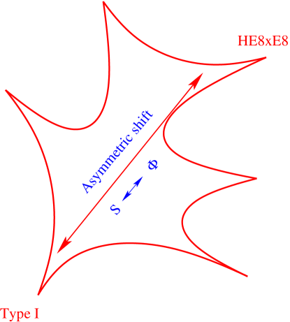
Figure 1: Implications from S–duality?

In this respect it is intriguing to consider what the incorporation of the asymmetric shift in the framework of M–theory dualities may imply. Under the strong–weak duality exchange between the heterotic–string and type I string, the dilaton is interchanged with a moduli. Hence, the possible implication of the asymmetric shift is that in the dual type I picture the dilaton VEV is fixed in the vicinity of the self–dual point. Naturally, this is an intriguing possibility, and hopefully it can be substantiated.

12 Back to T–duality

As discussed in section 2 a key property of string theory in compact space is the symmetry under exchange of a radius with its inverse, which is accompanied with exchange of momenta and winding modes. Reverting back to the wave–function of a free point particle in one dimension,

$$\Psi~{}\sim~{}{\rm e}^{iP\cdot X}~{},$$

we note that it is invariant under the exchange

$$P~{}\leftrightarrow~{}X.$$

However, in ordinary Kaluza–Klein compactification on a circle, we note that the invariance is lost due to the quantization of the momenta modes,

$$P={m\over R}.$$

In the case of the string, as discussed in section 2, we have that,

$$P~{}\sim~{}{m\over R}~{}+~{}nR.$$

If we think of the momenta and winding modes as the phase–space of the compact space, we have that the introduction of string winding modes restores this invariance. We can thus turn the table around and hypothesize that the key physical property that string theory enables is the restoration of the phase–space duality. Thus, the key physical property that should underly the formalism is the requirement of manifest phase–space duality. Furthermore, the phenomenological success of the free fermionic models, and their association with the self–dual points under T–duality, points to the possible association of the vacuum state of the theory with the self–dual state under phase–space duality. This view suggests a new starting point for the formulation of string theory and quantum gravity, and a constructive way to determine its vacuum. In the following I will describe the preliminary steps in such a program.

13 Phase–space duality

Duality and self–duality play a key role in the recent formulation of quantum mechanics from an equivalence postulate [55]. The duality in this context is phase–space duality, which is manifested due to the involutive nature of the Legendre transformation. Here I would like to demonstrate the association of the self–dual states under the phase–space duality with the states of vanishing kinetic and potential energy. Hence, again we note the relation between the self–duality criteria and the trivial state of the theory.

An instructive starting point to discuss the equivalence postulate approach to quantum mechanics is the classical Hamilton–Jacobi formalism. The classical Hamilton equations of motion

$$\dot{q}={\partial H\over\partial p},\qquad\dot{p}=-{\partial H\over\partial q},$$ (13.1)

are invariant under the transformations $p\rightarrow q$, $q\rightarrow-p$. However, in general in classical mechanics this duality is lost when a classical potential is specified. A viable question is therefore whether one can formulate classical mechanics with manifest phase–space duality. It turns out that phase–space duality cannot hold for all physical classical systems, and the break down is precisely for the states with vanishing energy and vanishing potential. The requirement that the phase–space duality holds for all physical system necessitates the quantum modification of classical mechanics [55]. In the Hamilton–Jacobi formalism of classical mechanics the phase–space variables are related by Hamilton’s generating function $p=\partial_{q}{S}_{0}(q)$. With the new generating function ${T}_{0}(p)$ defined by $q=\partial_{p}{T}_{0}$, the two generating functions are related by the dual Legendre transformations [55],

$${S}_{0}=p\partial_{p}{T}_{0}-{T}_{0}$$

and

$${T}_{0}=q\partial_{q}{S}_{0}-{S}_{0}.$$

Each of the Legendre transformations are related to a second differential equation [55] given in (13.4). Thus, we obtain the two dual pictures,

$$p={{\partial S_{0}}\over{\partial q}}~{}~{}~{}~{}~{}~{}~{}~{}~{}~{}~{}~{}~{}~{}~{}~{}~{}~{}~{}~{}~{}~{}~{} ~{}~{}~{}~{}~{}~{}~{}~{}~{}~{}~{}~{}~{}~{}q={{\partial T_{0}}\over{\partial p}},~{}~{}~{}~{}~{}~{}~{}~{}~{}~{}~{}~{}~{}~{}~{}~{}~{}~{}~{}~{}$$ , (13.2)

$$S_{0}=p{{\partial T_{0}\over\partial p}}-T_{0}~{}~{}~{}~{}~{}~{}~{}~{}~{}~{}~{}~{}~{}~{}~{} ~{}~{}~{}~{}~{}~{}~{}~{}~{}~{}~{}~{}~{}T_{0}=q{{\partial S_{0}\over\partial q}}-S_{0},$$ , (13.3)

$$\left({{\partial^{2}~{}~{}}\over\partial S_{0}^{2}}+U(S_{0})\right)\left({{q\sqrt{p}}\atop\sqrt{p}}\right)=0 ~{}~{}~{}~{}~{}~{}~{}~{}~{}~{}\left({{\partial^{2}~{}~{}}\over\partial T_{0}^{2}}+{\cal V}(T_{0})\right)\left({{p\sqrt{q}}\atop\sqrt{q}}\right)=0,~{}~{}~{}~{}~{}$$ , (13.4)

described by the two dual sets of differential equations. Two points are important to note. The first is that because the Legendre transformation is not defined for linear functions, i.e. for physical systems with ${S}_{0}=Aq+B$, it implies that the Legendre duality fails for the free system and for the free system with vanishing energy. Thus, we have the general condition that $S_{0}$ is never a linear function of the coordinate i.e.,

$$S_{0}~{}\neq~{}Aq~{}+~{}B~{}.$$

The second observation is that there exist a set of solutions, labeled by $pq=\gamma$, where $\gamma$ is a constant to be determined, which are simultaneous solutions of the two sets of differential equations. These are the self dual states under the phase–space duality, which are of the form [55],

$$S_{0}~{}\sim~{}\ln q.$$

14 The quantum equivalence postulate

The Legendre phase–space duality and its breakdown for the free system are intimately related to the equivalence postulate, which states that all physical systems labeled by the function ${W}(q)=V(q)-E$, can be connected by a coordinate transformation, $q^{a}\rightarrow q^{b}=q^{b}(q^{a})$, defined by

$${S}_{0}^{b}(q^{b})={S}_{0}^{a}(q^{a}).$$

This postulate implies that there always exist a coordinate transformation connecting any state to the state ${W}^{0}(q^{0})=0$. Inversely, this means that any physical state can be reached from the state ${W}^{0}(q^{0})$ by a coordinate transformation. This postulate cannot be consistent with classical mechanics. The reason being that in Classical Mechanics (CM) the state ${W}^{0}(q^{0})\equiv 0$ remains a fixed point under coordinate transformations. Thus, in CM it is not possible to generate all states by a coordinate transformation from the trivial state. Consistency of the equivalence postulate implies the modification of CM, which is analyzed by adding a still unknown function $Q$ to the Classical Hamilton–Jacobi Equation (CHJE). Consistency of the equivalence postulate fixes the transformation properties for ${W}(q)$,

$${W}^{v}(q^{v})=\left(\partial_{q^{v}}q^{a}\right)^{2}{W}^{a}(q^{a})+(q^{a};q^{v}),$$

and for $Q(q)$,

$$Q^{v}(q^{v})=\left(\partial_{q^{v}}q^{a}\right)^{2}Q^{a}(q^{a})-(q^{a};q^{v}),$$

which fixes the cocycle condition for the inhomogeneous term

$$(q^{a};q^{c})=\left(\partial_{q^{c}}q^{b}\right)^{2}[(q^{a};q^{b})-(q^{c};q^{b})].$$

The cocycle condition is invariant under Möbius transformations and fixes the functional form of the inhomogeneous term. The cocycle condition is generalizable to higher, Euclidean or Minkowski [55], dimensions, where the Jacobian of the coordinate transformation extends to the ratio of momenta in the transformed and original systems[55]. The identity

$$({\partial_{q}{S}_{0}})^{2}=\hbar^{2}/2\left(\{\exp(i2{S}_{0}/\hbar,q)\}-\{{S}_{0},q\}\right),$$

which embodies the equivalence postulate, leads to the Schrödinger equation. Making the identification

$${W}(q)=V(q)-E=-{\hbar^{2}/{4m}}\{{\rm e}^{(i2{S}_{0}/\hbar)},q\},$$ (14.1)

and

$${Q}(q)={\hbar^{2}/{4m}}\{{S}_{0},q\},$$

we have that ${S}_{0}$ is solution of the Quantum Stationary Hamilton–Jacobi Equation (QSHJE),

$$({1/{2m}})\left({{\partial_{q}S}_{0}}\right)^{2}+V(q)-E+({\hbar^{2}/{4m}})\{{S}_{0},q\}=0,$$ (14.2)

where $\{,\}$ denotes the Schwarzian derivative. From the identity we deduce that the trivializing map is given by $q\rightarrow{\tilde{q}}=\psi^{D}/\psi$, where $\psi^{D}$ and $\psi$ are the two linearly independent solutions of the corresponding Schrödinger equation [55, 56]. We see that the consistency of the equivalence postulate forces the appearance of quantum mechanics and of $\hbar$ as a covariantizing parameter.

15 The role of the self–dual states

The remarkable property of the QSHJE, which distinguishes it from the classical case, is that it admits non–trivial solution also for the trivial state, ${W}(q)\equiv 0$. Classical phase–space is described by the Classical Stationary Hamilton–Jacobi Equation (CSHJE)

$$({1/{2m}})\left({{\partial_{q}S}_{0}}\right)^{2}+V(q)-E=0.$$

The trivial solution, with

$$V(q)=0~{}~{},~{}~{}E=0,$$ (15.1)

is given by ,

$$S_{0}~{}=Aq+B,$$

i.e. precisely the solution which is not compatible with the Legendre duality transformation, which is not defined for linear functions. This solution is also incompatible with the equivalence postulate. On the other hand in the case of the quantum phase–space, which is described by the QSHJE (14.2), the state (15.1), admits a non–trivial solution. In fact the QSHJE implies that ${S}_{0}=constant$ is not an allowed solution. The fundamental characteristic of quantum mechanics in this approach is that ${S}_{0}\neq Aq+B$. Rather, the solution for the trivial state, with $V(q)=0$ and $E=0$, is given by

$${S}_{0}=i\hbar/2\ln q,$$

up to Möbius transformations. Remarkably, this quantum ground state solution coincides with the self–dual state of the Legendre phase–space transformation and its dual. Thus, we have that the quantum self–dual state plays a pivotal role in ensuring both the consistency of the equivalence postulate and definability of the Legendre phase–space duality for all physical states. The association of the self–dual state and the physical state with $V(q)=0$ and $E=0$ suggests a criteria by which the vacuum state of a given physical system could be identified. Namely, if one can identify correctly the complete phase–space and its duality structure, the vacuum state will then be identified with the self–dual states. Note also that the fact that the quantum potential is never vanishing, implies that even the trivial quantum state has a non–vanishing quantum potential.

16 Conclusions

String theory is in a precarious state of affairs. On the one hand the theory clearly exhibits great promise in providing a consistent framework for quantum gravity. On the other the need to embed the theory in higher dimensions is troubling. Furthermore, the apparent existence of a multitude of vacua, without an obvious mechanism to choose among them, led some authors to advocate the anthropic principle as a possible resolution for the contrived set of parameters that seem to govern our world.

The phenomenological approach to string theory advocates using the experimental data to study the properties of string theory. In this respect, it is likely that the type of backgrounds relevant for the physical observations differ from the generic backgrounds. For example the extra degrees of freedom needed to cancel the conformal anomaly will not appear as continuous dimensions, and hence their a priori geometrical interpretation may be misleading.

The string phenomenology program has by now been pursued for many years. A particular class of models that exhibit appealing phenomenological properties are the heterotic string models in the free fermionic formulation. A key property of this class of models is the relation of the free fermionic point in the moduli space and the self–dual point under T–duality. While the precise relationship needs to be better understood in the context of the realistic models, the self–dual point, being the symmetry point under T–duality, is the point where the moduli are likely to stabilize. Aside from being the symmetry point, the self–dual dual point is the one where the energy needed to excite the momenta and winding modes is minimized. It is rather obvious that a function which is invariant under exchange with its inverse has its minimum, for positive values, at the self–dual point.

The second key property of the realistic free fermionic models is their relation with $Z_{2}\times Z_{2}$ orbifold compactification. The special property of the $Z_{2}\times Z_{2}$ orbifold is that it acts on the internal coordinates as real rather than complex coordinates. This fact has important bearing on the problem of moduli fixing. In this context, recent work [4, 51, 54] revealed that the reduction to three generations in this class of models is achieved by utilizing an asymmetric identification between the left– and right–moving internal dimensions. The utilization of the asymmetric shift has the profound consequence that the untwisted geometrical moduli are projected out from the spectrum. Therefore, one should no longer regard the internal dimensions as generating ordinary geometrical objects. The precise nature of the underlying geometries requires further study and elucidation.

In the string phenomenology approach it is the data that is paving the way. This phenomenological work now opens new vistas that have been previously unforeseen. The notion of duality played a pivotal role in the theoretical developments in particle physics of the past two decades. Inspired by the phenomenological studies in the context of the free fermionic models, it was proposed here that phase–space duality is the guiding property in trying to formulate quantum gravity. In this respect T–duality is a key property of string theory. We can think of T-duality as a phase–space duality in the sense of exchanging momenta and winding modes in compact space. We can turn the table around and say that the key feature of string theory is that it preserves the phase–space duality in the compact space. It is further argued that the self–dual points under phase–space duality are intimately connected to the choice of the vacuum. The evidence for this arises from the phenomenological success of the free fermionic models that are constructed in the vicinity of the self–dual point, as well as from the formal derivation of quantum mechanics from phase–space duality and the equivalence postulate. It will be interesting to explore the notion of self–duality in the context of the modern nonperturbative duality studies. The framework of the Seiberg–Witten theory may provide a laboratory for such investigations in the sense that we may think of the curves of marginal stability [57] as the analog of the self–dual points. In this respect the enormous number of vacua in M–theory may be a mere reflection of the enormity of the gravitational quantum phase–space.

17 Acknowledgments

I would like to thank Ron Donagi, Costas Kounnas, Sander Nooij and John Rizos for collaboration and discussions. I would like to thank the Aspen Center for Theoretical Physics, The New High Energy Physics Group at Rutgers University, and the Institute for Advanced Study in Princeton for hospitality in the course of this work, This work was supported in part by a PPARC Advanced Fellowship, by the Royal Society, and by the EU networks, “Quest for Unification” and “Supersymmetry and the Early Universe”.

References

-
[1]
For review and references see e.g.:
M. Duff, hep-th/0403160; hep-th/9912164;
B. Ovrut, hep-th/0201032;
A. Sen, hep-th/0410103;
P. Townsend, hep-th/9612121. - [2] M.B. Green and J.H. Schwarz, Phys. Lett. B149 (1984) 117.
-
[3]
A.E. Faraggi, R. Garavuso and J.M. Isidro, Nucl. Phys. B641 (2002) 111; hep-th/0209245;
A.E. Faraggi and R. Garavuso, Nucl. Phys. B659 (2003) 224;
A.E. Faraggi and D.J. Clements, Int. J. Mod. Phys. A19 (2004) 2931. - [4] A.E. Faraggi, C. Kounnas, S.E.M. Nooij and J. Rizos, hep-th/0311058; Nucl. Phys. B695 (2004) 41.
- [5] For discussion and references see e.g.: H.P. Nilles, hep-th/0410160.
-
[6]
L. Susskind, hep-th/0302219;
M.R. Douglas, JHEP 0305 (2003) 046 ;
T. Banks, M. Dine, E. Gorbatov, JHEP 0408 (2004) 058 ; -
[7]
See e.g.:
M. Green, J. Schwarz and E. Witten, Superstring Theory, 2 vols., Cambridge University Press, 1987;
J. Polchinski, String Theory, 2 vols., Cambridge University Press, 1998;
C.V. Johnson, D–branes, Cambridge University Press, 2003. - [8] D.J. Gross, J.A. Harvey, E.J. Martinec and R, Rohm, Phys. Rev. Lett. 54 (1985) 502; Nucl. Phys. B256 (1985) 253; Nucl. Phys. B267 (1986) 75.
-
[9]
For review and references see e.g.:
A. Giveon, M. Porrati and E. Rabinovici, Phys. Rep. 244 (1994) 77. - [10] P. Ginsparg, Nucl. Phys. B295 (1988) 153
- [11] A. Giveon, E. Rabinovici and G. Veneziano, Nucl. Phys. B322 (1989) 167.
- [12] S. Elitzur, E. Gross, E. Rabinovici and N. Seiberg, Nucl. Phys. B283 (1987) 413.
- [13] See e.g.: C. Angelantonj and A. Sagnotti, Phys. Rep. 371 (2002) 1.
-
[14]
C. Vafa and E. Witten, 1996
Nucl.Phys.Proc.Suppl. 46 (1996) 225;
C. Angelantonj, I. Antoniadis and K. Förger, Nucl. Phys. B555 (1999) 116. - [15] A.E. Faraggi, Phys. Lett. B544 (2002) 207.
- [16] Y. Hosotani, Phys. Lett. B126 (83) 309; Phys. Lett. B129 (83) 193.
-
[17]
P. Candelas, G.T. Horowitz, A. Strominger and E. Witten,
Nucl. Phys. B258 (1985) 46;
M. Dine et al, Nucl. Phys. B259 (1985) 549;
B. Greene, K.H. Kirklin, P.J. Miron and G.G. Ross, Nucl. Phys. B278 (1986) 667; Nucl. Phys. B292 (1987) 606. -
[18]
E. Witten, Nucl. Phys. B268 (1986) 79;
J. Distler and S. Kachru, Nucl. Phys. B413 (1994) 213. - [19] L. Dixon, J. Harvey, C. Vafa and E. Witten, Nucl. Phys. B261 (1985) 678; Nucl. Phys. B274 (1986) 285.
-
[20]
K.S. Narain, Phys. Lett. B169 (1986) 41;
K.S. Narain, M.H. Sarmadi and E. Witten, Nucl. Phys. B279 (1987) 369. -
[21]
L. Ibanez, H.P. Nilles and F. Quevedo,
Phys. Lett. B187 (1987) 25;
J.A. Casas, E.K. Katehou, C. Munoz, Nucl. Phys. B317 (1989) 171;
A. Font, L. Ibanez, F. Quevedo and G. Sierra, Nucl. Phys. B331 (1990) 421;
J. Giedt, Annals Phys. 297 (2002) 67. -
[22]
A. Kagan and S. Samuel, Phys. Lett. B284 (1992) 289;
S. Chaudhuri, G. Hockney, J. Lykken, Nucl. Phys. B469 (1996) 357;
A.E. Faraggi, hep-th/9511093. - [23] S. Forste, H.P. Nilles, P.K.S. Vaudrevange and A. Wingerter, hep-th/0406208.
-
[24]
I. Antoniadis, C.P. Bachas and C. Kounnas, Nucl. Phys. B289 (1987) 87;
H. Kawai, D.C. Lewellen and S.H. Tye, Nucl. Phys. B288 (1987) 1. - [25] A.E. Faraggi, hep-ph/9707311; hep-th/9910042; hep-th/0208125; hep-th/0307037; hep-ph/0402029.
-
[26]
A.E. Faraggi and D.V. Nanopoulos, Phys. Rev. D48 (1993) 3288;
A.E. Faraggi, Int. J. Mod. Phys. A14 (1999) 1663. - [27] I. Antoniadis, J. Ellis, J. Hagelin and D.V. Nanopoulos, Phys. Lett. B231 (1989) 65.
- [28] I. Antoniadis, G. Leontaris and J. Rizos, Phys. Lett. B245 (1990) 161.
-
[29]
A.E. Faraggi, D.V. Nanopoulos and K. Yuan, Nucl. Phys. B335 (1990) 347;
A.E. Faraggi, Phys. Rev. D46 (1992) 3204. - [30] A.E. Faraggi, Phys. Lett. B278 (1992) 131; Nucl. Phys. B387 (1992) 239.
- [31] A.E. Faraggi, Phys. Lett. B274 (1992) 47; Phys. Lett. B377 (1995) 43; Nucl. Phys. B487 (1996) 55.
- [32] G.B. Cleaver et al, Phys. Lett. B455 (1999) 135; Int. J. Mod. Phys. A16 (2001) 425; Nucl. Phys. B593 (2001) 471; Mod. Phys. Lett. A15 (2000) 1191; Int. J. Mod. Phys. A16 (2001) 3565; Nucl. Phys. B620 (2002) 259.
- [33] G.B. Cleaver et al, Phys. Rev. D63 (2001) 066001; Phys. Rev. D65 (2002) 106003.
- [34] G.B. Cleaver, A.E. Faraggi and S.E.M. Nooij, Nucl. Phys. B672 (2003) 64.
- [35] S. Chang, C. Coriano and A.E. Faraggi, Phys. Lett. B397 (1997) 76; Nucl. Phys. B477 (1996) 65; J. Elwood and A.E. Faraggi, Nucl. Phys. B512 (1998) 42.
-
[36]
S. Chaudhuri et al, Nucl. Phys. B469 (1996) 357;
G.B. Cleaver et al, Nucl. Phys. B525 (1998) 3; Nucl. Phys. B545 (1998) 47; Phys. Rev. D59 (1999) 055005; Phys. Rev. D59 (1999) 115003 -
[37]
F. Abe et al, Phys. Rev. Lett. 74 (1995) 2626;
S. Abachi et al, Phys. Rev. Lett. 74 (1995) 2632. - [38] A.E. Faraggi, Nucl. Phys. B403 (1993) 101; Nucl. Phys. B407 (1993) 57
-
[39]
I. Antoniadis et al, Phys. Lett. B278 (1992) 257;
A.E. Faraggi and E. Halyo, Phys. Lett. B307 (1993) 305; Nucl. Phys. B416 (1994) 63;
J. Ellis et al, Phys. Lett. B425 (1998) 86 -
[40]
I. Antoniadis, J. Rizos and K. Tamvakis,
Phys. Lett. B279 (1992) 281;
A.E. Faraggi and E. Halyo, Phys. Lett. B307 (1993) 311;
A.E. Faraggi and J.C. Pati, Phys. Lett. B400 (1997) 314;
C. Coriano and A.E. Faraggi, Phys. Lett. B581 (2004) 99. -
[41]
I. Antoniadis, J. Ellis, R. Lacaze and D.V. Nanopoulos,
Phys. Lett. B268 (1991) 188;
I. Antoniadis, J. Ellis, S. Kelley and D.V. Nanopoulos, Phys. Lett. B272 (1991) 31;
A.E. Faraggi, Phys. Lett. B302 (1993) 202;
K.R. Dienes and A.E. Faraggi, Phys. Rev. Lett. 75 (1995) 2646; Nucl. Phys. B457 (1995) 409. -
[42]
A.E. Faraggi, Nucl. Phys. B428 (1994) 111;
Phys. Lett. B339 (1994) 223;
Phys. Lett. B398 (1997) 95;
Phys. Lett. B499 (2001) 147;
Phys. Lett. B520 (2001) 337;
J.C. Pati, Phys. Lett. B388 (1996) 532;
J. Ellis et al, Phys. Lett. B419 (1998) 123. -
[43]
I. Antoniadis, J. Ellis, A. Lahanas and D.V. Nanopoulos,
Phys. Lett. B241 (1990) 24;
A.E. Faraggi and E. Halyo, Int. J. Mod. Phys. A11 (1996) 2357;
A.E. Faraggi and J.C. Pati, Nucl. Phys. B526 (1998) 21;
A.E. Faraggi and O. Vives, Nucl. Phys. B641 (2002) 93. - [44] A. Dedes and A.E. Faraggi, Phys. Rev. D62 (2000) 016010.
-
[45]
A.E. Faraggi and D.V. Nanopoulos, Mod. Phys. Lett. A6 (1991) 61;
L.L. Everett, P. Langacker, M. Plumacher and J. Wang, Phys. Lett. B477 (2000) 233;
A.E. Faraggi and M. Thormeier, Nucl. Phys. B624 (2002) 163. -
[46]
X.G. Wen and E. Witten, Nucl. Phys. B261 (1985) 651;
K. Benakli, J. Ellis and D.V. Nanopoulos, Phys. Rev. D59 (1999) 047301;
S. Sarkar and R. Toldra, Nucl. Phys. B621 (2002) 495. - [47] A.E. Faraggi, K.A. Olive and M. Pospelov, Astrophys. J. 13 (2000) 31 .
-
[48]
C. Coriano and A.E. Faraggi, Phys. Rev. D65 (2002) 075001; hep-ph/0107304;
C. Corianò, A.E. Faraggi and M. Plumacher, Nucl. Phys. B614 (2001) 233;
A. Cafarella, C. Coriano and A.E. Faraggi, Int. J. Mod. Phys. A19 (2004) 3729; hep-ph/0306236. - [49] A.E. Faraggi, Phys. Lett. B326 (1994) 62.
- [50] P. Berglund et al, Phys. Lett. B433 (1998) 269; Int. J. Mod. Phys. A15 (2002) 1345.
- [51] R. Donagi and A.E. Faraggi, Nucl. Phys. B694 (2004) 187.
-
[52]
E. Kiritsis and C. Kounnas, Nucl. Phys. B503 (1997) 117;
A. Gregori, C. Kounnas and J. Rizos, Nucl. Phys. B549 (1999) 16. - [53] S.E.M. Nooij, University of Oxford D.Phil thesis.
- [54] A.E. Faraggi, C. Kounnas, S.E.M. Nooij and J. Rizos, paper in preparation.
-
[55]
A.E. Faraggi and M. Matone,
Phys. Rev. Lett. 78 (1997) 163;
Phys. Lett. B450 (1999) 34;
Phys. Lett. B437 (1998) 369;
Phys. Lett. A249 (1998) 180;
Phys. Lett. B445 (1998) 77;
Phys. Lett. B445 (1999) 357;
Int. J. Mod. Phys. A15 (2000) 1869;
G. Bertoldi, A.E. Faraggi and M. Matone, Class. Quant. Grav. 17 3965 (2000);
A.E. Faraggi, hep-th/0003156; hep-th/0312167. - [56] E.R. Floyd, Phys. Rev. D25 (1982) 1547; Phys. Rev. D26 (1982) 1339; Phys. Rev. D29 (1984) 1842; Phys. Rev. D34 (1986) 3246; Phys. Lett. A214 (1996) 259; Int. J. Mod. Phys. A14 (1999) 1111.
-
[57]
N. Seiberg and E. Witten, Nucl. Phys. B426 (1994) 19;
P.C. Argyres, A.E. Faraggi and A.D. Shapere, hep-th/9505190;
A. Bilal and F. Ferrari, Nucl. Phys. B480 (1996) 589;
A. Ritz, M.A. Shifman, A.I. Vainshtein and M.B. Voloshin, Phys. Rev. D63 (2001) 065018.