hep-th/0411067

Loop Operators and the Kondo Problem

Constantin Bachas$\ {}^{1,2}$ and Matthias R. Gaberdiel$\ {}^{2}$

$\ {}^{1}$ Laboratoire de Physique Théorique de l’Ecole Normale Supérieure
24 rue Lhomond, 75231 Paris cedex 05, France
 
$\ {}^{2}$ Institut für Theoretische Physik, ETH Hönggerberg
8093 Zürich, Switzerland
 
Email: bachas@lpt.ens.fr ; gaberdiel@itp.phys.ethz.ch

ABSTRACT

We analyse the renormalisation group flow for D-branes in WZW models from the point of view of the boundary states. To this end we consider loop operators that perturb the boundary states away from their ultraviolet fixed points, and show how to regularise and renormalise them consistently with the global symmetries of the problem. We pay particular attention to the chiral operators that only depend on left-moving currents, and which are attractors of the renormalisation group flow. We check (to lowest non-trivial order in the coupling constant) that at their stable infrared fixed points these operators measure quantum monodromies, in agreement with previous semiclassical studies. Our results help clarify the general relationship between boundary transfer matrices and defect lines, which parallels the relation between (non-commutative) fields on (a stack of) D-branes and their push-forwards to the target-space bulk.

LPTENS/04-46

November 2004

1 Introduction

The Kondo effect [1–6], i.e. the screening of magnetic impurities by the conduction electrons in a metal, has played a key role in the early development of the renormalisation group. More recently it has also proved instrumental in unraveling the elegant structure of boundary conformal field theory. In modern language, the screening describes the RG flow between the Cardy states [7] of the $\hat{su}(2)_{k}$ WZW model, where $k$ is the number of electron channels that participate in the process — see [8, 9] for reviews and further references.

In string theory conformal boundary states correspond to D-branes, and this has revived interest in the problem from a different, more geometrical point of view. It has been appreciated, in particular, that the symmetric WZW branes wrap (twisted) conjugacy classes of the group manifold [11, 12], that they are solutions of the Dirac-Born-Infeld equations [13, 14, 15], and that they are classified by an appropriate version of K-theory [16–20]. It was furthermore argued that the RG flow between different (stacks of) D-branes in these models is a process that lowers the energy by switching on certain non-abelian worldvolume backgrounds [24, 25]. This is similar to the dielectric effect for D-branes in the presence of a non-vanishing Ramond-Ramond field strength [26].

In a separate development [27] it was suggested that the choice of conformal boundary conditions in the WZW model amounts to the insertion of (spacelike) Wilson loops in the three-dimensional Chern-Simons theory. The approach was then generalised [28] to all rational CFTs, with Wilson loops replaced by more general ‘topological defect lines’. These were introduced in ref. [29] as formal bulk operators that commute with the chiral algebras of the theory. They are special cases of conformal defects, which in general only commute with the diagonal Virasoro algebra [30, 31, 32, 9]. Topological defects have been recently used to conjecture relations between boundary RG flows [33], and as generators of generalised Kramers-Wannier duality transformations [34].

Our aim in the present work will be to clarify the relation between these different approaches to the Kondo problem. We will work in the boundary state formalism [35, 36], and consider the renormalised transfer-matrix operator that perturbs the theory away from its ultraviolet fixed point. We will argue that this operator can be pushed forward smoothly into the bulk, so that it depends on left-moving currents only. As a result, it commutes with the right-moving algebra along the entire RG flow. At the infrared fixed point, this bulk operator also commutes with the left-moving algebra, and can be identified with the topological Wilson loops of ref. [27], or with the topological defect lines of ref. [29]. The fixed-point operator is in fact the trace of the quantum monodromy matrix [37–40]. Though we do not have a full proof, we will verify these statements explicitly at low orders in the perturbative expansion.

The existence of renormalisable loop operators, which can be moved freely to the boundary from the bulk, is a remarkable feature of the WZW model. It implies universal RG flows, common to all ultraviolet fixed points. From the geometric point of view, it means that the corresponding D-brane fields admit special, universal push-forwards to the entire target manifold. It would be very interesting to understand whether and, if so, how these features could be generalised to other models.

Besides those cited above, several other papers touch upon various aspects of our work. Most closely related is ref. [41], whose authors studied the same transfer-matrix operator and its action on WZW boundary states. Their analysis is, however, semiclassical, and they do not try to define the operator in the bulk, nor away from its critical point. The connection between quantum monodromy matrices and boundary flows has also been discussed by Bazhanov et.al. [42] in the context of minimal models. Their conformal perturbation scheme could be used in the Kondo problem, though it would force one to abandon the explicit $su(2)$ symmetry of the flow. Finally, other discussions of boundary states for D-branes with non-abelian backgrounds switched on can be found in refs. [43] and [44].

The plan of this paper is as follows : in section 2 we discuss the push-forward of D-brane fields to the bulk of the target space, and the corresponding push-forward of the boundary transfer matrix to a loop operator in the worldsheet bulk. We also explain the difference between conformal, chiral and topological defects. In section 3 we introduce the symmetric defect lines of the WZW model, and give a semiclassical argument that identifies their fixed points. In section 4 we regularise these defects, so as to respect a number of classical symmetries, and expand the regularised loop operator up to fourth order in the coupling constant. In section 5 we renormalise this operator and study its infrared fixed points. We verify explicitly at low orders that at the stable infrared fixed points, the operator commutes with the current algebra, and that its spectrum is given by generalised quantum dimensions. Finally in section 6 we pull back these operators to the boundary, and discuss the induced boundary RG flow. We end with some open questions.

2 Transfer matrices and defect lines

Consider a stack of $n$ identical D-branes in a target space parametrised by $X^{M}$. Let $n|\!|{\cal B}\rangle\!\rangle\$ be the conformal boundary state of the branes, with $A$ and $Y$ their matrix-valued gauge and coordinate fields. Switching on non-zero backgrounds for these fields leads to the following (formal) modification of the boundary state :

$$n\;|\!|{\cal B}\rangle\!\rangle\ \longrightarrow\;{\rm Tr}\;{\rm P}\;{\rm exp}\left(i\int_{0}^{2\pi}\hskip-0.28453ptd\sigma\left[A_{M}(X)\;\partial_{\sigma}X^{M}+{1\over 2\pi\alpha^{\prime}}\;Y_{M}(X)\;\partial_{\tau}X^{M}\right]\right)\;|\!|{\cal B}\rangle\!\rangle\ .$$ (2.1)

Here the integral runs over the boundary of the half-infinite cylinder that is parametrised by $\sigma\in[0,2\pi]$ and $\tau\in[0,\infty)$, the trace is over the Chan-Patton indices of $A$ and $Y$, and P denotes path ordering. The factor ${2\pi\alpha^{\prime}}$, conventional in the string-theory literature, could have been absorbed in the definition of $Y$. The worldsheet fields $X^{M}(\sigma,\tau)$ are quantised in the closed-string channel, i.e.  with $\tau$ being the time-like coordinate. The boundary at $\tau=0$ is thus spacelike and (barring singularities at coincident points) all worldsheet fields in expression (2.1) commute. The path ordering is, of course, still non-trivial because the background fields are matrix-valued.

The attentive reader will have noticed that we wrote $A$ and $Y$ as one-form fields, defined on the entire target manifold, ${\cal M}$, even though they live, a priori, only in the tangent (or normal) bundle of the D-brane worldvolume. What we implicitly assume is that the freedom in choosing this ‘push forward’ does not matter, because of the boundary conditions imposed by $|\!|{\cal B}\rangle\!\rangle$. Consider for example a D-instanton at the origin, whose boundary state satisfies the conditions $X^{M}(\sigma,0)|\!|{\cal B}\rangle\!\rangle\,=\,0$. Ignoring problems of operator ordering, one would conclude that the integrand in (2.1) reduces to $Y_{M}(0)\partial_{\tau}X^{M}/2\pi\alpha^{\prime}$, so that only the value of $Y$ at the origin really matters. This is of course a semiclassical argument, and it is possible that it fails at the quantum level.

A closely-related question is the following. The path-ordered exponential in eq. (2.1) is the closed-string dual of the transfer matrix, or evolution operator in the open channel. Let us denote this operator by ${\cal O}(A,Y)$. If we were to quantise $X^{M}$ with $\sigma$ as time, then ${\cal O}$ would be the evolution operator in the interaction representation, around the theory defined by the boundary condition ${\cal B}$. From this perspective, only the action of ${\cal O}$ on the boundary state $|\!|{\cal B}\rangle\!\rangle$ is really specified. Extending the action of the path-ordered exponential to all closed-string states requires a push-forward of $A$ and $Y$ to the whole target manifold. This makes it, in turn, possible to push the integration contour from the boundary to the interior of the worldsheet, where boundary conditions are no more effective (see figure 1). Reversing this operation amounts to taking the limit

$${\rm lim}_{\varepsilon\to 0}\;{\cal O}(A,Y)\;e^{i\varepsilon(L_{0}+\bar{L}_{0})}|\!|{\cal B}\rangle\!\rangle\ ,$$ (2.2)

where $L_{0}+\bar{L}_{0}$ is the Hamiltonian in the closed-string channel. If the limit is non-singular, it should only depend on the pullbacks of $A$ and $Y$ to the tangent and normal bundles of the original, unperturbed D-brane.

                         

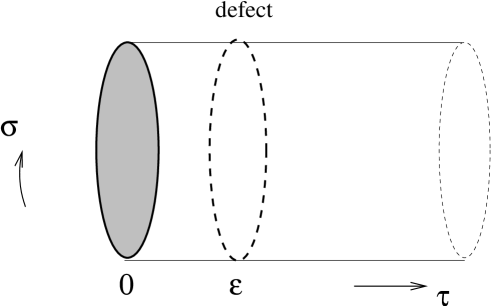
Figure 1: A push-forward of the D-brane fields to the target manifold, makes it possible to push the integration contour of (2.1) from the boundary to the interior of the worldsheet.

In the open channel, the operator ${\cal O}(A,Y)$ describes the interactions of a point defect sitting in the interior of the worldsheet. Such defects have been previously discussed in the condensed-matter [30, 9] and in the string-theory [31, 32] literature. By folding the worldsheet along their worldline, one may picture bulk defects geometrically as D-branes in the tensor product, ${\cal M}\times{\cal M}$, of two identical target manifolds. The trivial defect, i.e. the identity operator, corresponds to the diagonal brane in ${\cal M}\times{\cal M}$ [31, 32]. Its geometric and gauge degrees of freedom are precisely given by two one-form fields living on ${\cal M}$. This fits very nicely with the fact that $A_{M}(x)$ and $Y_{M}(x)$ account (together with the tachyon field) for the most general renormalisable couplings on a defect worldline.

Conformal defects are obtained at the fixed points $(A^{*},Y^{*})$ of the RG flow. The corresponding loop operators commute with the generators of conformal transformations that preserve the defect worldline,

$$\left[\;{\cal L}_{n}\;,\;{\cal O}(A^{*},Y^{*})\;\right]\;=0\ \ \ \ \ \forall\;n\ ,$$ (2.3)

where ${\cal L}_{n}=L_{n}-\bar{L}_{-n}\$ with $L_{n}$ and $\bar{L}_{n}$ the left- and right-moving Virasoro generators, respectively. [Note in particular that ${\cal L}_{0}$ generates translations in $\sigma$.] It follows from conditions (2.3) that if $|\!|{\cal B}\rangle\!\rangle$ is a conformal boundary state, i.e. if it is annihilated by all ${\cal L}_{n}$, then ${\cal O}(A^{*},Y^{*})|\!|{\cal B}\rangle\!\rangle$ is also conformal. Thus, if the limit (2.2) were smooth, pulling back the RG flow of a bulk defect to any conformal boundary would induce a (possibly trivial) RG flow of the boundary state. Conformal defect lines, in particular, act as solution-generating symmetries, i.e.  they map conformal to conformal boundary states.

In general, taking the limit (2.2) can be tricky, since the presence of the boundary could conceivably modify the RG flow at distances much greater than $\varepsilon$. There exists, however, one special class of defects that commute with the right-moving Virasoro algebra,

$$\left[\;{\bar{L}}_{n}\;,\;{\cal O}_{\rm chir}(A,Y)\;\right]\;=0\ ,$$ (2.4)

and for which the limit (2.2) is trivial. We will refer to them as chiral defects (or anti-chiral if they commute with the left-moving algebra). Chiral defects need not be conformal, but they can be regularised and renormalised in a way that preserves their invariance under $\sigma$-translations. They therefore commute with both ${\cal L}_{0}$ and $\bar{L}_{0}$, and hence also with the closed-string Hamiltonian. Thus, chiral defects can be taken freely to the boundary of the cylinder, where they induce RG flows of boundary states.

Defect lines that are both conformal and chiral correspond to operators that commute with both the left and the right Virasoro algebras,

$$\left[\;{L}_{n}\;,\;{\cal O}_{\rm chir}(A^{*},Y^{*})\;\right]\;=\left[\;{\bar{L}}_{n}\;,\;{\cal O}_{\rm chir}(A^{*},Y^{*})\;\right]\;=0\ .$$ (2.5)

We will call such defect lines topological, since their action only depends on the homotopy class of the integration contour. The corresponding operator will be denoted for short by ${\cal O}_{\rm top}$. The conditions (2.5), together with a Cardy constraint of integral multiplicities, have been used in ref. [29] to give an algebraic definition of (topological) defect lines. Notice that the Cardy constraint is automatically obeyed provided ${\cal O}_{\rm top}$ is the transfer matrix for some local defect. Note also that ${\cal O}_{\rm top}$ need not be continuously connected (in D-brane configuration space) to the identity operator. What can be asserted, following ref. [33], is that if $|\!|{\cal B}\rangle\!\rangle\to|\!|{\cal B}^{\prime}\rangle\!\rangle$ is an allowed boundary RG flow, then so is ${\cal O}_{\rm top}|\!|{\cal B}\rangle\!\rangle\to{\cal O}_{\rm top}|\!|{\cal B}^{\prime}\rangle\!\rangle$ for any topological-defect operator. This observation gives support for the flows that have been proposed in [49, 50].

Simple examples of topological defect operators are the generators of continuous symmetries, ${\cal O}_{\rm top}={\rm exp}(i\lambda\oint J)$ with $\lambda$ a real parameter and $J$ any abelian chiral spin-$1$ current. Another set includes discrete automorphisms of the CFT, as analyzed in ref. [34]. Both of these types of operators are invertible, and do not arise as infrared fixed points of RG flows, in contrast to the Kondo problem operators that we will study here.

3 Semiclassical analysis of WZW defects

One may identify conformal defects in the WZW model by a semiclassical argument, analogous to the one used to argue for the existence of a conformal theory in the bulk [51]. We recall the expressions for the left- and right-moving currents of the model,

$$J(x^{+})=-i\kappa\;(\partial_{+}g)g^{-1}\ \ \ {\rm and}\ \ \ \ \bar{J}(x^{-})=i\kappa\;g^{-1}\partial_{-}g\ ,$$ (3.1)

where $x^{\pm}=\tau\pm\sigma$, and $g(x^{+},x^{-})$ takes values in some (simple compact) Lie group $G$. The parameter $\kappa$ is related to the integer level $k$ through

$$\kappa=\psi^{2}k/2\ ,$$ (3.2)

with $\psi$ the length of long roots of the Lie algebra $g$ of $G$. The currents generate the independent left and right symmetry transformations

$$g\to u(x^{+})^{-1}\;g\;\bar{u}(x^{-})\ ,$$ (3.3)

under which they themselves transform as :

$$J\to u^{-1}Ju+i\kappa\;u^{-1}\partial_{+}u\qquad\ {\rm and}\qquad\bar{J}\to\bar{u}^{-1}\bar{J}\bar{u}+i\kappa\;\bar{u}^{-1}\partial_{-}\bar{u}\ .$$ (3.4)

The Poisson bracket algebra of the Fourier moments, $J_{n}^{a}$, of these currents is the classical counterpart of the standard left- and right-moving affine Kac-Moody algebras $\hat{g}$ with central extension $k$. This algebra implies the transformation rules (3.4), and vice versa.

We will be interested in bulk defects which interact linearly with the currents of the model, and preserve a global $G$ symmetry. The classical observable that corresponds to the quantum transfer matrix of such defects reads

$${\cal O}_{\omega}(\lambda,\bar{\lambda};R)={\rm Tr}_{R}\;{\rm P\;exp}\;\left(i\int_{0}^{2\pi}d\sigma\;(\lambda\;J^{a}\;-\;\bar{\lambda}\;\omega(\bar{J}^{a}))\;t^{a}\right)\ .$$ (3.5)

Here $t^{a}$ are the generators of $g$ in an $n$-dimensional irreducible representation $R$, $\omega$ is an automorphism of the Lie algebra $g$, $\lambda$ and $\bar{\lambda}$ are independent real coupling constants, and there is an implicit sum over the adjoint index $a$. It will be useful to consider (3.5) as the Wilson loop of a two-dimensional gauge field with components

$$(\alpha_{+},\alpha_{-})\;=\;(\;\lambda\;J^{a}t^{a}\;,\;\bar{\lambda}\;\omega(\bar{J}^{a})t^{a}\;)\ .$$ (3.6)

By virtue of the non-abelian Stokes theorem, the observables (3.5) are conserved under the (closed-string) time evolution, provided that the field strength $F_{+-}=i\;[\alpha_{+},\alpha_{-}]$ vanishes. This is however not the case in general, except for chiral (or antichiral) defects for which the coupling $\bar{\lambda}$ (or $\lambda$) is zero.

Let us concentrate on the chiral defects, with Wilson loops

$${\cal O}_{\rm chir}(\lambda;R)={\rm Tr}_{R}\;{\rm P\;exp}\;\left(i\lambda\oint_{C}dx^{+}\;J^{a}t^{a}\right)\ .$$ (3.7)

Classically, such Wilson loops are topological, i.e. they only depend on the homotopy class of the contour $C$. This property does not, a priori, survive the renormalisation process, which introduces through dimensional transmutation a length scale. There is however one special value of the coupling,

$$\lambda^{*}=-{1\over\kappa}\ ,$$ (3.8)

for which ${\cal O}_{\rm chir}(\lambda^{*};R)$ is in fact invariant under the full symmetries (3.4) of the WZW model. To see why, recall that a Wilson loop is invariant under the gauge transformations

$$\alpha_{\pm}\to v^{-1}\alpha_{\pm}v-iv^{-1}\partial_{\pm}v$$ (3.9)

for arbitrary $v(x^{+},x^{-})$. The transformation (3.4) of $\ (\lambda^{*}J^{a}t^{a}\;,\;0)\$ is of precisely this same form with $v(x^{+},x^{-})=u(x^{+})$. An immediate consequence is that this special Wilson loop has vanishing Poisson brackets with both current algebras,

$$\{J_{n}^{a}\;,\;{\cal O}_{\rm chir}(\lambda^{*};R)\}_{\;{}_{\rm PB}}=\{\bar{J}_{n}^{a}\;,\;{\cal O}_{\rm chir}(\lambda^{*};R)\}_{\;{}_{\rm PB}}=0\ .$$ (3.10)

As we will verify in the following sections, to lowest order in $1/\kappa$ these relations do survive the canonical correspondence $\{\;,\;\}_{\;{}_{\rm PB}}\to[\;,\;]\$ (though in general $\lambda^{*}$ has a finite, scheme-dependent renormalisation). Since the Virasoro generators are quadratic in the affine currents, ${\cal O}_{\rm chir}(\lambda^{*};R)$ will thus also obey eq. (2.5) that characterises topological defects.

The above semiclassical argument can help us identify another class of defects, which are conformal but not topological. They correspond to the symmetric choice

$$\lambda=\bar{\lambda}={\lambda^{*}\over 2}\ .$$ (3.11)

With this choice, the observables (3.5) are invariant under the (vector-like) transformations that have $u(x)=\omega(\bar{u}(-x))$, as the reader can easily verify. These vector-like transformations are generated by the linear combinations of currents

$${\cal J}_{n}^{a}=J_{n}^{a}+\omega(\bar{J}_{-n}^{a})\ ,$$ (3.12)

which must therefore have vanishing Poisson brackets with the loop observables,

$$\left\{{\cal J}_{n}^{a}\;,\;{\cal O}_{\omega}\left({\lambda^{*}\over 2},{\lambda^{*}\over 2};R\right)\right\}_{\;{}_{\rm PB}}=0\ \ .$$ (3.13)

Note that the ${\cal J}_{n}^{a}$ define a current algebra without central extension. Now assuming that (3.13) survives in the quantum theory, and recalling that the Virasoro generators are quadratic in the currents and $\omega$-invariant, we immediately conclude that ${\cal O}_{\omega}(\lambda^{*}/2,\lambda^{*}/2;R)$ will obey the defining relations (2.3) of conformal defects. Note, however, that these defect lines are not topological — they do not, in particular, commute with the $\tau$-evolution. In fact, they correspond, as we shall later see, to unstable fixed points of the RG flow.

The topological observables ${\cal O}_{\rm chir}(\lambda^{*};R)$, together with their right-moving counterparts, measure the invariant monodromies of classical solutions. More explicitly, a general solution of the classical WZW equations factorises into the product of a left- and a right-moving part,

$$g(x^{+},x^{-})=g_{+}(x^{+})^{-1}g_{-}(x^{-})\ .$$ (3.14)

Since only $g$ needs to be a single-valued function on the worldsheet, one has

$$g_{\pm}(x^{\pm}\pm 2\pi)=Mg_{\pm}(x^{\pm})\ ,$$ (3.15)

with $M$ an arbitrary but constant group element. As the reader can easily check,

$${\cal O}_{\rm chir}(\lambda^{*};R)={\rm Tr}_{R}\;M\ ,$$ (3.16)

where the trace is evaluated in the $R$ representation. Note that the decomposition (3.14) is not unique — the freedom to redefine $g_{\pm}=g_{0}\;g_{\pm}\$, with $g_{0}$ an arbitrary constant group element, changes $M$ to $g_{0}Mg_{0}^{-1}$. This is compatible with the fact that our topological observables only measure the conjugacy class of the monodromy.

Using the above freedom, one can bring $g_{\pm}$ to the canonical form

$$g_{\pm}=e^{\pm i\Lambda\;x^{\pm}}\;\tilde{g}_{\pm}(x^{\pm})\,,$$ (3.17)

where $\tilde{g}_{\pm}$ are single-valued functions on the circle, $M=e^{2\pi i\Lambda}$ is the monodromy matrix, and $\Lambda$ can be chosen (by a Weyl reflection) to lie in a positive Cartan alcove of $\hat{g}$. The triplet $(\tilde{g}_{+},\tilde{g}_{-},\Lambda)$ describes the classical phase space of the WZW model. A geometric quantization of this phase space, known as co-adjoint orbit or Kirillov-Konstant quantization [38, 39, 40] (see also [52]), gives the following spectrum for the monodromy :

$$\Lambda={\mu+\rho\over k+h^{\vee}}\,\ \ \ \ {\rm in\ the\ sector}\ \ {\cal H}_{\mu}\otimes\bar{\cal H}_{\mu}\ .$$ (3.18)

Here ${\cal H}_{\mu}$ and $\bar{\cal H}_{\mu}$ are integrable highest-weight representations of the left and right current algebras, respectively; they are labelled by a highest weight vector $\mu$ of the corresponding representation of $g$. Furthermore, $\rho$ is the Weyl vector of $g$, i.e. one half of the sum of all positive roots of $g$. Semiclassical reasoning does not actually determine the finite shift of $k$ by the dual Coxeter number $h^{\vee}$ — a detailed quantum calculation is needed for this. Using (3.18) one finds the following spectrum for the topological defect operator,

$${\cal O}_{\rm chir}(\lambda^{\ast};R)={\rm Tr}_{R}\left(e^{2\pi i\Lambda}\right)={S_{R\mu}\over S_{0\mu}}\,\ \ \ \ \ {\rm in\ \ }{\cal H}_{\mu}\otimes\bar{\cal H}_{\mu}\ .$$ (3.19)

Here $S$ is the modular transformation matrix of the chiral characters, and $0$ (and $R$) denotes the Kac-Moody representation built on the trivial (or the $R$) representation of $g$. Note that the trace of $M$ in the above expression can be computed for an arbitrary representation $R$, not only for those corresponding to integrable representations of the current algebra.

We end this section with some remarks. Firstly, the topological defect lines (3.19) should ‘lift’ to the (spacelike) Wilson lines of the 3d Chern-Simons theory [27], but it is not clear whether a lift exists for the more general, non-topological defects. Second, the above loop observables define a classical (fusion) algebra,

$${\cal O}_{\omega}(\lambda,\bar{\lambda};R_{1})\;{\cal O}_{\omega}(\lambda,\bar{\lambda};R_{2})=\sum_{R\in R_{1}\otimes R_{2}}{\cal O}_{\omega}(\lambda,\bar{\lambda};R)\ ,$$ (3.20)

for any values of the coupling constants. It would be interesting to know whether this algebra structure survives at the quantum level. Finally, the symmetric defects discussed here form a special class, and do not exhaust all conformal defects of WZW models.

4 Regularised loop operators

As a first step towards quantising the defect lines of the previous section, we will now describe a regularisation scheme and write ${\cal O}_{\omega}^{\rm reg}(\lambda,\bar{\lambda};R)$ as an operator in the enveloping algebra of the current algebras. We start by defining the regularised left-moving currents

$$J_{\rm reg}^{a}(\sigma)=\sum_{n\in{\bf Z}}J^{a}_{n}\;e^{-in\sigma-|n|s/2}\,,$$ (4.1)

where $s$ is a short-distance cutoff, and the $J^{n}_{a}$ are generators of the Kac-Moody algebra

$$[J^{a}_{n},J^{b}_{m}]=if^{abc}\;J^{c}_{n+m}+{\kappa}\,n\;\delta^{ab}\delta_{n+m,0}\ .$$ (4.2)

A similar expression defines the regularised right-moving currents. Note that this regulator preserves the classical algebra of analytic symmetry transformations, i.e. transformations generated by positive-frequency modes of the currents.

Let us concentrate first on chiral defects, and expand the loop observables (3.7) in a power series of the coupling constant,

$${\cal O}_{\rm chir}(\lambda;R)=\sum_{N=0}^{\infty}{(i\lambda)^{N}}\;{\cal O}^{(N)}(R)\ ,$$ (4.3)

where

$${\cal O}^{(N)}(R)={\rm Tr}_{R}\;(t^{a_{1}}\cdots t^{a_{N}})\left(\prod_{i=1}^{N}\int_{0}^{2\pi}d\sigma_{i}\right)\;\theta_{\sigma_{1}>\cdots>\sigma_{N}}\;J^{a_{1}}(\sigma_{1})\cdots J^{a_{N}}(\sigma_{N})\;$$ (4.4)

with $\theta_{\sigma_{1}>\cdots>\sigma_{N}}=1$ if $\sigma_{1}>\sigma_{2}\cdots>\sigma_{N}$, and $\theta_{\sigma_{1}>\cdots>\sigma_{N}}=0$ otherwise. Classically, the order of the currents in the above expression is irrelevant, but in the quantum theory a precise order must be specified. To guide our choice we will insist that the following two symmetries of the classical observables be preserved: (i) the path can start at any point $\sigma_{0}$ on the circle, and (ii) the result is invariant if we reverse the orientation of the loop, and change $R$ with its conjugate representation. Neither of these symmetries would be preserved if we kept the order of the currents as in (4.4). However, these symmetries are preserved if we average over the $N$ cyclic permutations, as well as the $N$ permutations that are obtained from them by reversing the order, i.e. by combining them with the permutation $\rho:j\mapsto N+1-j$. We thus define

$${\cal O}_{\rm reg}^{(N)}(R)={\rm Tr}_{R}\;(t^{a_{1}} \hskip-14.22636pt\cdots t^{a_{N}})\left(\prod_{i=1}^{N}\int_{0}^{2\pi}d\sigma_{i}\right)\;\theta_{\sigma_{1}>\cdots>\sigma_{N}}\times$$

$$\qquad\qquad\times{1\over 2N}\left(J_{\rm reg}^{a_{1}}(\sigma_{1})\cdots J_{\rm reg}^{a_{N}}(\sigma_{N})\;+{\rm cyclic}\ +{\rm reversal}\right)\ .$$

Note that since the bare currents at non-coincident points commute, the choice of ordering is part of the regularisation prescription for the loop operator. Note also that our prescription (which is not unique) guarantees that ${\cal O}_{\rm reg}^{(N)}(R)$ commutes with the generator of $\sigma$-translations. As explained in the previous section, such chiral operators can be transported freely to the boundary of the half-infinite cylinder.

Plugging the mode decomposition (4.1) in (4), and performing explicitly the integrals leads to the following expressions for the first few values of $N$ :

$${\cal O}_{\rm reg}^{(2)}(R)=2\pi^{2}\;{\rm Tr}_{R}(t^{a}t^{b})\;J_{0}^{a}J_{0}^{b}\ ,$$ (4.6)

$${\cal O}_{\rm reg}^{(3)}(R)={2\pi^{2}\over 3}\;{\rm Tr}_{R}(t^{a}t^{b}t^{c})\left[\,{\pi\over 3}\;J_{0}^{a}J_{0}^{b}J_{0}^{c}+\sum_{n\not=0}{i\over n}\tilde{J}^{a}_{-n}\tilde{J}^{b}_{n}J^{c}_{0}\;+{\rm cyclic}+{\rm reversal}\;\right]\ ,$$ (4.7)

and

$${\cal O}_{\rm reg}^{(4)}(R) = {\pi^{2}\over 2}\;{\rm Tr}_{R}(t^{a}t^{b}t^{c}t^{d})\;\Biggl{[}\,{\pi^{2}\over 6}\;J_{0}^{a}J_{0}^{b}J_{0}^{c}J^{d}_{0}\,+\,\sum_{n\not=0}{i\pi\over n}\tilde{J}^{a}_{-n}\tilde{J}^{b}_{n}J^{c}_{0}J^{d}_{0}$$

$$\quad+\sum_{n\not=0}{1\over n^{2}}\,\left(\tilde{J}^{a}_{-n}\tilde{J}^{b}_{n}J^{c}_{0}J^{d}_{0}-\tilde{J}^{a}_{-n}J^{b}_{0}\tilde{J}^{c}_{n}J^{d}_{0}\right)+\sum_{\stackrel{{\scriptstyle\footnotesize{m,l,n\not=0}}}{{m+n+l=0}}}{1\over ml}\,\tilde{J}^{a}_{m}\tilde{J}^{b}_{n}\tilde{J}^{c}_{l}J^{d}_{0}$$

$$\quad-{1\over 2}\sum_{m,n\not=0}{1\over mn}\tilde{J}^{a}_{-n}\tilde{J}^{b}_{n}\tilde{J}^{c}_{-m}\tilde{J}^{d}_{m}\;+\;{\rm cyclic}+{\rm reversal}\;\Biggr{]}\ .$$

Here we have used the short-hand notation $\tilde{J}^{a}_{n}=J^{a}_{n}\;e^{-|n|s/2}$. Note that in deriving these formulae it helps to sum over all cyclic permutations of the currents and use the cyclic property of the trace, before performing explicitly the $\sigma_{j}$ integrals.

Let us pause for a moment to describe our group theoretic conventions. The $t^{a}$ are (traceless) generators of $g$ in the representation $R$, which we assume irreducible. The Killing form is $\delta^{ab}$, so adjoint indices can be raised and lowered freely. We denote by ${\rm dim}(R)$ the dimension of $R$, and by $C(R)$ the value of the quadratic Casimir operator in the representation $R$, i.e. $\sum_{a}t^{a}t^{a}=C(R)\times{\rm identity}$. In these conventions

$${\rm Tr}_{R}\;(t^{a}t^{b})=I_{R}\,\delta^{ab}\ ,\ \ \ {\rm where}\ \ \ \ I_{R}={C(R)\times{\rm dim}(R)\over{\rm dim}(g)}\ ,$$ (4.9)

where ${\rm dim}(g)$ is the dimension of the adjoint representation. Furthermore, the dual Coxeter number $h^{\vee}$ is given by :

$$I_{adj}\;\delta^{ab}=\sum_{a,b}f^{abc}f^{abd}=h^{\vee}\psi^{2}\delta^{ab}\,,$$ (4.10)

where $\psi^{2}$ is the length squared of the longest root. We will also need the trace of triple products of generators,

$${\rm Tr}_{R}\;(t^{a}t^{b}t^{c}) = {1\over 2}\;{\rm Tr}_{R}([t^{a},t^{b}]t^{c})+{1\over 2}\;{\rm Tr}_{R}(\{t^{a},t^{b}\}t^{c})$$ (4.11)

$$= {i\over 2}\,f^{abc}\,I_{R}+{1\over 2}\,d^{abc}\,I_{R}^{(3)}\,,$$

where $d^{abc}$ is the totally symmetric invariant third order tensor, and $I_{R}^{(3)}$ is related to the value in the representation $R$ of the associated third order Casimir operator,

$$C_{3}=\sum_{abc}d^{abc}\,t^{a}\,t^{b}\,t^{c}\ .$$ (4.12)

Note that the $d^{abc}$ may vanish, as happens for example for $su(2)$. The first non-trivial case, $su(3)$, will be described in more detail at the end of section 5.

After normal ordering the expressions (4.6– 4), i.e. moving all positive modes to the right of negative modes, and with the help of the above trace formulae we find :

$${\cal O}_{\rm reg}^{(2)}(R)=2\pi^{2}I_{R}\;J_{0}^{a}J_{0}^{a}\,,$$ (4.13)

$${\cal O}_{\rm reg}^{(3)}(R) = {2\pi^{3}\over 3}\,I_{R}^{(3)}\,d^{abc}\,J^{a}_{0}J^{b}_{0}J^{c}_{0}\;+\;4\pi^{2}I_{R}\;f^{abc}\sum_{n>0}{1\over n}\;J^{a}_{-n}J^{b}_{0}J^{c}_{n}\;-$$

$$-\;4\pi^{2}i\;I_{R}\,h^{\vee}\,\psi^{2}\left[\;\sum_{n>0}{1\over n}J^{a}_{-n}J^{a}_{n}\,-\,{1\over 2}\,J^{a}_{0}J^{a}_{0}\left(\sum_{n>0}{e^{-ns}\over n}\right)\,+\,{\kappa\,\over 6}\,{\rm dim}(g)\;\left(\sum_{n>0}e^{-ns}\right)\right]\,,$$

and

$${\cal O}_{\rm reg}^{(4)}(R) = :{\cal O}_{\rm reg}^{(4)}(R):-\;2\pi^{2}\,I_{R}\,h^{\vee}\,\psi^{2}\,\kappa\,\Biggl{[}\;\sum_{n>0}{1\over n}\;J^{a}_{-n}J^{a}_{n}-\,J^{a}_{0}J^{a}_{0}\;\left(\sum_{n>0}{e^{-ns}\over n}\right)\,+$$ (4.15)

$$+\;{\kappa\over 4}\,{\rm dim}(g)\,\left(\sum_{n>0}e^{-ns}\right)\Biggr{]}\;\ +\;\ {\rm subleading}\,.$$

For the quartic operator we have not written out explicitly the ‘subleading terms’ that arise in the process of normal ordering if one uses at least once the $if^{abc}$ piece of the current commutators. These terms have fewer powers of $J\sim\kappa^{1/2}$, and they depend on the precise definition of the normal ordered expression $:{\cal O}_{\rm reg}^{(4)}(R):$. Indeed, different definitions of $:{\cal O}_{\rm reg}^{(4)}(R):$ differ by rearrangements of the positive, or of the negative modes, which only involve the $if^{abc}$ piece of the commutator.

We have only calculated those ‘subleading’ terms that make divergent contributions (in the $s\to 0$ limit) to the quadratic and cubic Casimir operators of $G$. Put differently, if we write

$${\cal O}_{\rm chir}^{\rm reg}(\lambda;R)\,=\,\cdots+A_{2}(\lambda;R)\,J_{0}^{a}J_{0}^{a}\,+\,A_{3}(\lambda;R)\,d^{abc}J_{0}^{a}J_{0}^{b}J_{0}^{c}+\cdots\ ,$$ (4.16)

then the coefficients $A_{2}$ and $A_{3}$ read :

$$A_{2}(\lambda;R)\,=-2\pi^{2}I_{R}\,\left[\lambda^{2}+\lambda^{3}\xi+\lambda^{4}\left(\kappa\,\xi+{3\over 4}\,\xi^{2}+{\rm finite}\right)+O(\lambda^{5})\right]\$$ (4.17)

and

$$A_{3}(\lambda;R)\,=\,-{2\pi^{3}i\over 3}\;I_{R}^{(3)}\;\left[\lambda^{3}+\lambda^{4}\,\left({3\over 2}\,\xi+{\rm finite}\right)+O(\lambda^{5})\right]\ ,$$ (4.18)

where we have defined

$$\xi=h^{\vee}\psi^{2}\,{\rm log}\,s\,.$$ (4.19)

In calculating these results, we made use of the infinite sums

$$\sum_{n=1}^{\infty}e^{-ns}={1\over s}-{1\over 2}+O(s)\ \ \ \quad\ \ \ \sum_{n=1}^{\infty}{e^{-ns}\over n}=-{\rm log}s+O(s)\ ,$$ (4.20)

and dropped terms that vanish as $s\to 0$.

Our discussion of regularised operators can be extended easily to the non-chiral defects of section 3. Regularising the operator ${\cal O}_{\omega}(\lambda,\bar{\lambda};R)$ like ${\cal O}_{\rm chir}(\lambda;R)$ leads to the same expressions as (4.6–4), except for the replacement (for say $\omega=1$)

$$\lambda\tilde{J}_{n}^{a}\ \longrightarrow(\lambda J_{n}^{a}-\bar{\lambda}\bar{J}_{-n}^{a})\,e^{-|n|s/2}\ .$$ (4.21)

Left and right currents are normal-ordered separately, giving expressions like (4.13–4.15), which we will not explicitly write down. Note that the sum of frequencies in each term does not have to add up to zero now, since non-chiral operators do not commute with the Hamiltonian in the closed-string channel.

5 Renormalisation and fixed points

Based on symmetry arguments, we expect that the divergent contributions to the chiral operators of the previous section can be absorbed into a redefinition of two parameters : the coupling $\lambda$ and an overall multiplicative factor. These correspond to the two local counterterms, proportional to the identity and to $J^{a}t^{a}$, that have dimension $\leq 1$ and respect the chiral and the global $G$-symmetries of the problem. Alternatively, the only two background fields consistent with these symmetries are a constant tachyon, and $A=Y$ proportional to the right-invariant one-form on $G$. This huge reduction of parameter space implies that by choosing $\lambda_{\rm eff}$ and $Z_{R}$ appropriately, we should be able to take the limit

$${\cal O}_{\rm chir}^{\rm ren}(\lambda_{\rm eff};R)\;=\;{\rm lim}_{s\to 0}\;Z_{R}\;{\cal O}_{\rm chir}^{\rm reg}(\lambda;R)\ .$$ (5.1)

Close inspection of eqs. (4.3) and (4.13 – 4.18) shows that this is the case up to the order worked out in section 4. A possible choice of the multiplicative renormalisation and of the effective coupling, that removes all divergencies to this order, is :

$$\lambda_{\rm eff}=\lambda+{1\over 2}(\lambda^{2}+\kappa\lambda^{3})\,\xi+{1\over 4}\,\lambda^{3}\,\xi^{2}+O(\lambda^{4})\ ,$$ (5.2)

and

$${\rm log}\,Z_{R}=2\,\pi^{2}\,C(R)\,h^{\vee}\,\psi^{2}\,\left(\,{1\over 3}\,\kappa\lambda^{3}+{1\over 4}\,\kappa^{2}\lambda^{4}+{\rm subleading}\right)\times{1\over s}\ ,$$ (5.3)

where subleading stands for higher powers of $\lambda\sim 1/\kappa$ (this scaling is of interest for reasons that will be discussed in a minute). Note that, as anticipated in our notation, $\lambda_{\rm eff}$ is independent of the representation $R$, while ${\rm log}Z_{R}$ depends on it (to this order) via the eigenvalue of the quadratic Casimir operator. Note also that $s$ is the ratio of the only two length scales in the problem: the short-distance cutoff and the circumference, ${L}$, of the cylinder. Subtracting minimally the $s$ pole, as in (5.3), is tantamount to a renormalisation of the energy of the defect that only depends on the cutoff scale, and not on $L$. This same subtraction would have been automatically implemented by the $\zeta$-function regularisation

$$\sum_{n>0}1=\zeta(0)=-{1\over 2}\,.$$ (5.4)

From equations (5.2) and (4.19) we can now extract the $\beta$-function

$$\beta(\lambda_{\rm eff})=-{d\lambda_{\rm eff}\over d\,{\rm log}s}=-{1\over 2}h^{\vee}\psi^{2}\left(\lambda_{\rm eff}^{2}+\kappa\lambda_{\rm eff}^{3}+O(\lambda_{\rm eff}^{4})\right)\,.$$ (5.5)

The chiral defect is asymptotically free, and has an infrared fixed point at the critical value

$$\lambda^{*}=-{1\over\kappa}+O\left({1\over\kappa^{2}}\right)\ .$$ (5.6)

This agrees with the semiclassical argument of section 3 in the $\kappa>\!\!>1$ region. The fact that the fixed point is close to the origin justifies the use of perturbation theory in his limit. Note, incidentally, that in the renormalisation scheme we have used the two-loop $\beta$-function is proportional to $\kappa$.

It is straightforward to extend this calculation to the general non-chiral defect (3.5). To leading order in the $\lambda\sim\bar{\lambda}\sim 1/\kappa$ expansion, the effective couplings in this case read

$$\lambda_{\rm eff} = \lambda+{1\over 2}\,\xi\,\left(\lambda^{2}+\kappa(\lambda^{3}+\lambda\,\bar{\lambda}^{2})\right)+\cdots$$

$$\bar{\lambda}_{\rm eff} = \bar{\lambda}+{1\over 2}\,\xi\,\left(\bar{\lambda}^{2}+\kappa(\bar{\lambda}^{3}+\bar{\lambda}\,\lambda^{2})\right)+\cdots\ .$$

The corresponding RG flow is described by the flow diagram of Figure 2. As is manifest from this diagram, there are three non-trivial fixed points: the stable chiral and anti-chiral fixed points at $(\lambda,\bar{\lambda})=(-1/\kappa,0)$ and $(0,-1/\kappa)$, as well as an unstable fixed point at $\lambda=\bar{\lambda}=-1/2\kappa$. This is again in nice agreement with the expectations based on the quasiclassical analysis of section 3.

                                 

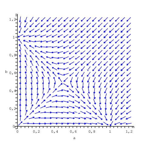
Figure 2: The RG flow diagram for the general symmetric defects discussed in the text. The space of couplings is parametrised by $(a,b)=-\kappa(\lambda,\bar{\lambda})$. The stable fixed points correspond to chiral defects, but there is also an unstable fixed point along the line $\lambda=\bar{\lambda}$ .

As was furthermore argued in section 3, the fixed-point operators ${\cal O}_{\rm chir}(\lambda^{*};R)$ are non-trivial central elements of the (left-moving) current algebra that take the value $S_{R\mu}/S_{0\mu}$ on the highest weight representation ${\cal H}_{\mu}$. We now want to confirm these statements to the order to which we have calculated ${\cal O}_{\rm chir}^{\rm ren}(\lambda^{*};R)$, and this will occupy us in the remainder of the present section. The reader may choose to skip these cumbersome calculations, and proceed directly to the following section.

Let us first verify to lowest order that ${\cal O}_{\rm chir}^{\rm ren}(\lambda^{*};R)$ is central, i.e. that it commutes with all Kac-Moody generators $J_{n}^{e}$. Since at the fixed point $\lambda=\lambda_{\rm eff}+O(\kappa^{-3})$, and since $Z_{R}$ is only a multiplicative factor, it will be sufficient to check this for the regularised bare expressions. The contribution from the second-order term is :

$$-{\lambda^{2}}[\,J^{e}_{n}\,,{\cal O}_{\rm reg}^{(2)}(R)] = -2\pi^{2}\lambda^{2}\,I_{R}\,if^{eab}\left(J^{b}_{n}J^{a}_{0}+J^{a}_{0}J^{b}_{n}\right)$$ (5.7)

$$= -4\pi^{2}\lambda^{2}\,I_{R}\,\left(if^{eab}J^{a}_{0}J^{b}_{n}+{1\over 2}\,h^{\vee}\psi^{2}\,J^{e}_{n}\right)\,.$$

This needs to be cancelled by corresponding contributions from third and fourth order. Since $\lambda\sim 1/\kappa$, the relevant contributions from the third-order term must be proportional to $\kappa$. These must come from the central term of the commutator involving $J^{e}_{n}$, and will only arise for $n\neq 0$ [for $n=0$ note that (5.7) vanishes, and so do all the other commutators because of the global $G$-symmetry of the defect line]. The relevant contributions read

$$-i{\lambda^{3}}[\,J^{e}_{n}\,,{\cal O}_{\rm reg}^{(3)}(R)]=-4\pi^{2}\,\lambda^{3}\kappa\,I_{R}\left(if^{eab}\,J^{a}_{0}J^{b}_{n}+h^{\vee}\psi^{2}J^{e}_{n}\right)+\cdots\,.$$ (5.8)

Provided we choose $\lambda=-1/\kappa$, the term that is bilinear in $J$ cancels. The term linear in $J$, on the other hand, is cancelled by a contribution at fourth order

$${\lambda^{4}}[\,J^{e}_{n},{\cal O}_{\rm reg}^{(4)}(R)]=-2\pi^{2}\lambda^{4}\,\kappa^{2}\,I_{R}\,h^{\vee}\psi^{2}\,J^{e}_{n}+\cdots\,.$$ (5.9)

Thus, at the fixed point all terms in (5.7) – (5.9) cancel precisely, and there are no further contributions at order $\kappa^{-2}$. Indeed, if it were to contribute at this order, the commutator of ${\cal O}_{\rm reg}^{(N)}(R)$ with $J^{e}_{n}$ would have to be proportional to $\kappa^{N-2}$. Since two $J$s are needed to produce a power of $\kappa$, the only option is $N=5$, but then the resulting term would not involve any $J$s any more. This is impossible because the total mode number of any ${\cal O}_{\rm reg}^{(N)}(R)$ is zero, so that the commutator with $J^{e}_{n}$ must involve modes whose mode numbers sum to $n\neq 0$.

Let us now turn to the verification of the semiclassical formula (3.19). Since ${\cal O}_{\rm chir}^{\rm ren}(\lambda^{*};R)$ commutes with the current algebra, it is sufficient to calculate its eigenvalue on the (conformal) highest weight state $|\mu\rangle$ in ${\cal H}_{\mu}$. Using equations (4.13–4.15) and (5.1–5.3) we find :

$${\cal O}_{\rm chir}^{\rm ren}(\lambda;R)\,|\mu\rangle = \Biggl{[}\,\dim(R)\,-\,2\pi^{2}\,\lambda^{2}\,I_{R}\,C(\mu)\,-\,{2i\pi^{3}\over 3}\,\lambda^{3}\,I^{(3)}_{R}\,C_{3}(\mu)\,+$$ (5.10)

$$\hskip-56.9055pt+\,\pi^{2}\,\left({\kappa\over 3}\,\lambda^{3}\,+{\kappa^{2}\over 4}\,\lambda^{4}\,\right)I_{R}\,h^{\vee}\,\psi^{2}\,\dim(g)\,+\,{\rm subleading}\,\Biggr{]}\,|\mu\rangle\,,$$

where we are neglecting terms of order $\kappa\lambda^{4}J$ and $\lambda^{4}J^{3}$, and of course all terms of order $\lambda^{5}$. Note that $C(\mu)$ and $C_{3}(\mu)$ denote the values of the quadratic and cubic Casimir operators in the representation $\mu$ (see section 4).

Plugging into this formula the critical value (5.6) one finds :

$${\cal O}_{\rm chir}^{\rm ren}(\lambda^{*};R)\,|\mu\rangle=\left[\dim(R)-{2\pi^{2}\over\kappa^{2}}\,I_{R}\,C(\mu)-{\pi^{2}\over 12\kappa^{2}}\,I_{R}\,h^{\vee}\,\psi^{2}\,\dim(g)+{O}\left({1\over\kappa^{3}}\right)\right]\,|\mu\rangle\,.$$ (5.11)

The expression in brackets agrees precisely with the expansion of the generalised quantum dimension ${S_{R\mu}/S_{0\mu}}$ up to cubic order. We can in fact do still a little better: the terms that we did not calculate explicitly in (5.10) cannot contribute to the coefficient of the quadratic or cubic Casimir at order $\kappa^{-3}$ (but can only modify the constant term at this order). If we assume that the critical value of the coupling constant is shifted in the familiar way,

$$\lambda^{\ast}=-{1\over\kappa+h^{\vee}\psi^{2}/2}+O\left({1\over\kappa^{3}}\right)\ ,$$ (5.12)

then (5.10) actually reproduces the coefficients of the quadratic and cubic Casimir of ${S_{R\mu}/S_{0\mu}}$ even up to cubic order, at least for $su(2)$ and $su(3)$. For $su(2)$ this is simply a consequence of the fact that $I_{R}^{(3)}=0$, and that the generalised quantum dimensions are even functions of $k+2$. In the case of $su(3)$, we use the fact (see for example [55]) :

$$d^{abc}{\rm Tr}_{R}(t^{a}t^{b}t^{c})=\dim(R)\,C_{3}(R)=I_{R}^{(3)}\,d^{abc}\,d^{abc}={40\over 3}\,I_{R}^{(3)}\,,$$ (5.13)

where we have here set $\psi^{2}=1$. It follows that the order $\kappa^{-3}$ contribution of (5.10) at the critical value of the coupling (5.12) is equal to :

$$-{i\,\pi^{3}\over 20\,\kappa^{3}}\,\dim(R)\,C_{3}(R)\,C_{3}(\mu)\,.$$ (5.14)

If we describe the representation $\mu$ by the Dynkin labels $[\mu_{1},\mu_{2}]$, then the cubic Casimir operator reads (see for example reference [56], which uses however a different normalisation convention from ours) :

$$C_{3}(\mu)={1\over 36}\,(\mu_{1}-\mu_{2})\,(\mu_{1}+2\mu_{2}+3)\,(\mu_{2}+2\mu_{1}+3)\,.$$ (5.15)

Substituting this into (5.14) reproduces the cubic contribution of the generalised quantum dimension for $su(3)$, as can be checked explicitly by using the description of the $S$-matrix elements given in ref. [57].

6 Boundary RG flows

Finally, we can now return to our original problem, which concerned the renormalisation group flow of boundary states. The main point we want to stress is the following : since the renormalised loop operators have been constructed in the bulk, their action on the boundary defines universal RG flows, independent of the ultraviolet brane $n|\!|{\cal B}\rangle\!\rangle$. Conformal defect lines, in particular, define (generally non-invertible) maps in the space of conformal boundary states, i.e. they act as solution-generating symmetries of open string theory. What this means geometrically is that there exist universal bundles, $A$ and $Y$, on the target space which solve the open-string equations if pulled back on any classically consistent brane. Note that unlike the continuous or discrete automorphisms of the CFT, these maps change in general the tension (or $g$-function) of the D-brane. Note also that the universality of the flows may shed light on the empirical observation that the charge groups of the untwisted and twisted D-branes always coincide [20].

The endpoint of the boundary RG flow induced by the symmetric WZW defects of this paper, is given by the action of the loop operator at one of the three non-trivial fixed points of figure 2. Let us consider first the chiral case. Most of what we describe in the following is well known to the experts (see for example [29, 33]), but we include it for completeness. The space of states of the closed string theory describing strings on the simply-connected group manifold $G$ is

$${\cal H}=\bigoplus_{\mu\in P^{+}_{k}(g)}{\cal H}_{\mu}\otimes\bar{\cal H}_{\mu^{\ast}}\,,$$ (6.16)

where $P^{+}_{k}(g)$ denotes the set of integrable highest weight representations of the affine algebra $\hat{g}$ at level $k$. The D-branes that preserve the affine symmetry up to the (possibly trivial) automorphism $\omega$ are characterised by the gluing condition

$$\left[J^{a}_{n}+\omega\left(\bar{J}^{a}_{-n}\right)\right]\,|\!|\alpha\rangle\!\rangle=0\,.$$ (6.17)

As always, these D-branes can be expanded in terms of the corresponding Ishibashi states

$$|\!|\alpha\rangle\!\rangle=\sum_{\mu\in{\cal E}_{\omega}}{\psi_{\alpha\mu}\over\sqrt{S_{0\mu}}}\,|\mu\rangle\!\rangle^{\omega}\,,$$ (6.18)

where $|\mu\rangle\!\rangle^{\omega}$ is the unique Ishibashi state satisfying (6.17) in the sector ${\cal H}_{\mu}\otimes\bar{\cal H}_{\mu^{\ast}}$, and ${\cal E}_{\omega}$ denotes the set of exponents, i.e.

$${\cal E}_{\omega}=\left\{\mu\in P^{+}_{k}(g):\omega(\mu)=\mu\right\}\,.$$ (6.19)

The D-branes are then uniquely characterised by the unitary matrix $\psi_{\alpha\mu}$. For an introduction to these matters see for example [58].

For the case $\omega={\rm id}$, ${\cal E}_{\omega}=P^{+}_{k}(g)$, and the D-branes are naturally labelled by the integrable highest weight representations of $\hat{g}$. The matrix $\psi_{\alpha\mu}=S_{\alpha\mu}$ is then the modular $S$-matrix, and the corresponding D-branes are sometimes referred to as the ‘Cardy branes’. If $\omega$ is non-trivial, the D-branes are often called the ‘twisted’ D-branes; they are naturally labelled by the $\omega$-twisted representations of the affine algebra, and the $\psi$-matrix is then the modular transformation matrix describing the modular transformation of twisted and twined characters [59, 60]. In either case, the open string that stretches between the branes labelled by $\beta$ and $\alpha$ then contains the representation ${\cal H}_{\nu}$ of $\hat{g}$ with multiplicity

$${\cal N}_{\nu\alpha}{}^{\beta}=\sum_{\mu\in{\cal E}_{\omega}}{\psi_{\alpha\mu}\,S_{\nu\mu}\,\psi_{\beta\mu}^{\ast}\over S_{0\mu}}\,.$$ (6.20)

The consistency of the construction requires that these numbers are non-negative integers, and in fact, they must define a NIM-rep of the fusion algebra – see e.g. [58, 61] for an introduction to these matters.

We are interested in studying the action of the chiral loop operator on the boundary state labelled by $\alpha$. Since the loop operator only involves the left-moving modes $J^{a}_{n}$, it obviously commutes with the right-moving modes $\bar{J}^{a}_{m}$ for any value of the (renormalised) coupling constant $\lambda$. We have argued above that for the critical coupling, $\lambda=\lambda^{\ast}$, the operator also commutes with the left-moving currents $J^{a}_{n}$. Thus at the critical coupling, the loop operator maps a boundary state satisfying (6.17) to another boundary state satisfying (6.17). We want to calculate this resulting boundary state.

At the critical coupling, the loop operator commutes with all modes $J^{a}_{n}$, and therefore must act as a $C$-number on each irreducible representation ${\cal H}_{\mu}$ of $\hat{g}$. As we have argued before, this $C$-number is precisely equal to the generalised quantum dimension

$$\left.{\cal O}_{\rm chir}^{\rm ren}(\lambda^{*};R)\right|_{{\cal H}_{\mu}}={S_{R\mu}\over S_{0\mu}}\,.$$ (6.21)

Thus we find

$${\cal O}_{\rm chir}^{\rm ren}(\lambda^{*};R)\,|\!|\alpha\rangle\!\rangle=\sum_{\mu\in{\cal E}_{\omega}}{S_{R\mu}\over S_{0\mu}}\,{\psi_{\alpha\mu}\over\sqrt{S_{0\mu}}}\,|\mu\rangle\!\rangle^{\omega}\,.$$ (6.22)

For each $\mu\in{\cal E}_{\omega}$ we write

$${S_{R\mu}\over S_{0\mu}}\,{\psi_{\alpha\mu}\over\sqrt{S_{0\mu}}} = \sum_{\beta}{\psi_{\beta\mu}\over\sqrt{S_{0\mu}}}\sum_{\nu\in{\cal E}_{\omega}}{\psi^{\ast}_{\beta\nu}S_{R\nu}\psi_{\alpha\nu}\over S_{0\nu}}$$ (6.23)

$$= \sum_{\beta}{\psi_{\beta\mu}\over\sqrt{S_{0\mu}}}\,{\cal N}_{R\alpha}{}^{\beta}\,,$$

where the unitarity of $\psi_{\alpha\nu}$ was used in the first line, i.e.

$$\sum_{\beta}\psi^{\ast}_{\beta\nu}\,\psi_{\beta\mu}=\delta_{\nu\mu}\,,$$ (6.24)

with both $\mu$ and $\nu$ elements of ${\cal E}_{\omega}$. In the second line we have inserted the definition of the NIM-rep coefficient (6.20). Putting this back into (6.22) we then find

$${\cal O}_{\rm chir}^{\rm ren}(\lambda^{*};R)\,|\!|\alpha\rangle\!\rangle=\sum_{\beta}{\cal N}_{R\alpha}{}^{\beta}\,|\!|\beta\rangle\!\rangle\,.$$ (6.25)

This therefore reproduces the flow that was proposed in [16], based on the analysis of the non-commutative worldvolume actions [24, 25] and the Kondo problem [6, 8]. These flows were used in [16, 17, 18] to show that the untwisted branes carry the charge that was predicted by K-theory; for the twisted D-branes this was shown in [20].

In the diagonal theories discussed above, the actions of the chiral and antichiral operators coincide. This is also true (semiclassically at least) for the non-chiral operator ${\cal O}_{\omega}^{\rm ren}(\lambda^{\ast}/2,\lambda^{\ast}/2;R)$, if the gluing automorphism of the ultraviolet brane is the same as the one that goes into the definition of the defect line. More generally, the combination of defect and boundary breaks the global $G$ symmetry of the problem. The pull-back of the defect to the boundary may, in this case, be singular, corresponding to the excitation of modes that take us outside the original two-parameter space of couplings. This raises the more general problem of the fusion between arbitrary defect and boundary flows; for topological defect lines this question was analysed in ref. [33].

The analysis of this paper can be extended easily to the D-branes of any bulk theory in which left and/or right current algebras exist. Examples include WZW models of non-simply connected group manifolds, as well as WZW orbifolds and coset models in which part of the current algebras survives. It is less clear whether the above ideas can be applied to more general coset models, or to the D-branes of WZW models for non-compact groups. These questions deserve further investigation.

Acknowledgements

This research has been partially supported by the European Networks ‘Superstring Theory’ (HPRN-CT-2000-00122) and ‘The Quantum Structure of Spacetime’ (HPRN-CT-2000-00131), as well as by the Swiss National Science Foundation. We have benefited from discussions with Anton Alekseev, Giovanni Felder, Stefan Fredenhagen, Jürg Fröhlich, Terry Gannon, Kryzstof Gawedzki, Hanno Klemm, Ruben Minasian, Boris Pioline, Ingo Runkel, Volker Schomerus, Samson Shatashvili, Jan Troost and Sasha Zamolodchikov. We also thank the organisers of the Ascona workshop, where part of the work has been carried out.

References

- [1] J. Kondo, “Resistance minimum in dilute magnetic alloys,” Prog. Theor. Phys. 32 (1964) 37.
- [2] P. Nozières, “A Fermi-liquid description of the Kondo problem at low temperatures,” J. Low. Temp. Phys. 17 (1974) 31.
- [3] K.G. Wilson, “The renormalization group: critical phenomena and the Kondo problem,” Rev. Mod. Phys. 47 (1975) 773.
- [4] N. Andrei, “Diagonalization of the Kondo Hamiltonian,” Phys. Rev. Lett. 45 (1980) 379.
- [5] P.B. Wiegmann, “Exact solution of exchange model at ,” JETP Lett. 31 (1980) 392.
- [6] I. Affleck and A.W.W. Ludwig, “The Kondo effect, conformal field theory and fusion rules,” Nucl. Phys. B 352 (1991) 849 ; “Critical Theory Of Overscreened Kondo Fixed Points,” Nucl. Phys. B 360 (1991) 641 ; “Exact critical theory of the two impurity Kondo model,” Phys. Rev. Lett. 68 (1992) 1046.
- [7] J.L. Cardy, “Boundary conditions, fusion rules and the Verlinde formula,” Nucl. Phys. B 324 (1989) 581.
- [8] I. Affleck, “Conformal field theory approach to the Kondo effect,” Acta Phys. Polon. B 26 (1995) 1869 [arXiv:cond-mat/9512099].
- [9] H. Saleur, “Lectures on non perturbative field theory and quantum impurity problems,” parts I and II, arXiv:cond-mat/9812110 and cond-mat/0007309.
- [10] G. Pradisi, A. Sagnotti and Y.S. Stanev, “Planar duality in SU(2) WZW models,” Phys. Lett. B 354 (1995) 279 [arXiv:hep-th/9503207]; “The open descendants of nondiagonal SU(2) WZW models,” Phys. Lett. B 356 (1995) 230 [arXiv:hep-th/9506014]; “Completeness conditions for boundary operators in 2D conformal field theory,” Phys. Lett. B 381 (1996) 97 [arXiv:hep-th/9603097].
- [11] A.Yu. Alekseev and V. Schomerus, “D-branes in the WZW model,” Phys. Rev. D 60 (1999) 061901 [arXiv:hep-th/9812193].
- [12] G. Felder, J. Fröhlich, J. Fuchs and C. Schweigert, “The geometry of WZW branes,” J. Geom. Phys. 34 (2000) 162 [arXiv:hep-th/9909030].
- [13] C. Bachas, M.R. Douglas and C. Schweigert, “Flux stabilization of D-branes,” JHEP 0005 (2000) 048 [arXiv:hep-th/0003037].
- [14] J. Pawelczyk, “SU(2) WZW D-branes and their noncommutative geometry from DBI action,” JHEP 0008 (2000) 006 [arXiv:hep-th/0003057].
- [15] P. Bordalo, S. Ribault and C. Schweigert, “Flux stabilization in compact groups,” JHEP 0110 (2001) 036 [arXiv:hep-th/0108201].
- [16] S. Fredenhagen and V. Schomerus, “Branes on group manifolds, gluon condensates, and twisted K-theory,” JHEP 0104 (2001) 007 [arXiv:hep-th/0012164].
- [17] J.M. Maldacena, G.W. Moore and N. Seiberg, “D-brane instantons and K-theory charges,” JHEP 0111 (2001) 062 [arXiv:hep-th/0108100].
- [18] P. Bouwknegt, P. Dawson and A. Ridout, “D-branes on group manifolds and fusion rings,” JHEP 0212 (2002) 065 [arXiv:hep-th/0210302].
- [19] V. Braun, “Twisted K-theory of Lie groups,” JHEP 0403 (2004) 029 [arXiv:hep-th/0305178].
- [20] M.R. Gaberdiel and T. Gannon, “The charges of a twisted brane,” JHEP 0401 (2004) 018 [arXiv:hep-th/0311242].
- [21] R. Minasian and G.W. Moore, “K-theory and Ramond-Ramond charge,” JHEP 9711 (1997) 002 [arXiv:hep-th/9710230].
- [22] E. Witten, “D-branes and K-theory,” JHEP 9812 (1998) 019 [arXiv:hep-th/9810188].
- [23] P. Bouwknegt and V. Mathai, “D-branes, B-fields and twisted K-theory,” JHEP 0003 (2000) 007 [arXiv:hep-th/0002023].
- [24] A.Yu. Alekseev, A. Recknagel and V. Schomerus, “Brane dynamics in background fluxes and non-commutative geometry,” JHEP 0005 (2000) 010 [arXiv:hep-th/0003187].
- [25] A.Yu. Alekseev, S. Fredenhagen, T. Quella and V. Schomerus, “Non-commutative gauge theory of twisted D-branes,” Nucl. Phys. B 646 (2002) 127 [arXiv:hep-th/0205123].
- [26] R.C. Myers, “Dielectric-branes,” JHEP 9912 (1999) 022 [arXiv:hep-th/9910053].
- [27] G. Felder, J. Fröhlich, J. Fuchs and C. Schweigert, “Conformal boundary conditions and three-dimensional topological field theory,” Phys. Rev. Lett. 84 (2000) 1659 [arXiv:hep-th/9909140]; “Correlation functions and boundary conditions in RCFT and three-dimensional topology,” Compos. Math. 131 (2002) 189 [arXiv:hep-th/9912239].
- [28] J. Fuchs, I. Runkel and C. Schweigert, “TFT construction of RCFT correlators. I: Partition functions,” Nucl. Phys. B 646 (2002) 353 [arXiv:hep-th/0204148]; “Boundaries, defects and Frobenius algebras,” Fortsch. Phys. 51 (2003) 850 [Annales Henri Poincare 4 (2003) S175] [arXiv:hep-th/0302200].
- [29] V.B. Petkova and J.B. Zuber, “Generalised twisted partition functions,” Phys. Lett. B 504 (2001) 157 [arXiv:hep-th/0011021].
- [30] M. Oshikawa and I. Affleck, “Boundary conformal field theory approach to the critical two-dimensional Ising model with a defect line,” Nucl. Phys. B 495 (1997) 533 [arXiv:cond-mat/9612187].
- [31] C. Bachas, J. de Boer, R. Dijkgraaf and H. Ooguri, “Permeable conformal walls and holography,” JHEP 0206 (2002) 027 [arXiv:hep-th/0111210].
- [32] T. Quella and V. Schomerus, “Symmetry breaking boundary states and defect lines,” JHEP 0206 (2002) 028 [arXiv:hep-th/0203161].
- [33] K. Graham and G.M.T. Watts, “Defect lines and boundary flows,” JHEP 0404 (2004) 019 [arXiv:hep-th/0306167].
- [34] J. Fröhlich, J. Fuchs, I. Runkel and C. Schweigert, “Kramers-Wannier duality from conformal defects,” Phys. Rev. Lett. 93 (2004) 070601 [arXiv:cond-mat/0404051].
- [35] C.G. Callan, C. Lovelace, C.R. Nappi and S.A. Yost, “Adding holes and crosscaps to the superstring,” Nucl. Phys. B 293 (1987) 83; “Loop corrections to superstring equations of motion,” Nucl. Phys. B 308 (1988) 221.
- [36] J. Polchinski and Y. Cai, “Consistency of open superstring theories,” Nucl. Phys. B 296 (1988) 91.
- [37] O. Babelon, “Extended conformal algebra and Yang-Baxter equation,” Phys. Lett. B 215 (1988) 523.
- [38] A.Yu. Alekseev and S.L. Shatashvili, “Quantum groups and WZW Models,” Commun. Math. Phys. 133 (1990) 353.
- [39] K. Gawedzki, “Classical origin of quantum group symmetries in Wess-Zumino-Witten conformal field theory,” Commun. Math. Phys. 139 (1991) 201.
- [40] M. Chu, P. Goddard, I. Halliday, D.I. Olive and A. Schwimmer, “Quantization of the Wess-Zumino-Witten model on a circle,” Phys. Lett. B 266 (1991) 71.
- [41] Y. Hikida, M. Nozaki and Y. Sugawara, “Formation of spherical D2-brane from multiple D0-branes,” Nucl. Phys. B 617 (2001) 117 [arXiv:hep-th/0101211].
- [42] V.V. Bazhanov, S.L. Lukyanov and A.B. Zamolodchikov, “Integrable structure of conformal field theory, quantum KdV theory and thermodynamic Bethe ansatz,” Commun. Math. Phys. 177 (1996) 381 [arXiv:hep-th/9412229]; “Integrable structure of conformal field theory II. Q-operator and DDV equation,” Commun. Math. Phys. 190 (1997) 247 [arXiv:hep-th/9604044].
- [43] N. Ishibashi, “p-branes from (p-2)-branes in the bosonic string theory,” Nucl. Phys. B 539 (1999) 107 [arXiv:hep-th/9804163]; “A relation between commutative and noncommutative descriptions of D-branes,” arXiv:hep-th/9909176.
- [44] I. Pesando, “Multibranes boundary states with open string interactions,” arXiv:hep-th/0310027.
- [45] C.P. Bachas and M.R. Gaberdiel, “World-sheet duality for D-branes with travelling waves,” JHEP 0403 (2004) 015 [arXiv:hep-th/0310017].
- [46] C. Bachas, “Relativistic string in a pulse,” Annals Phys. 305 (2003) 286 [arXiv:hep-th/0212217].
- [47] Y. Hikida, H. Takayanagi and T. Takayanagi, “Boundary states for D-branes with traveling waves,” JHEP 0304 (2003) 032 [arXiv:hep-th/0303214].
- [48] P.T. Matthews, “The application of the Tomonaga-Schwinger theory to the interaction of nucleons with central scalar and vector mesons,” Phys. Rev. 76 (1949) 1657.
- [49] S. Fredenhagen and V. Schomerus, “On boundary RG-flows in coset conformal field theories,” Phys. Rev. D 67 (2003) 085001 [arXiv:hep-th/0205011].
- [50] S. Fredenhagen, “Organizing boundary RG flows,” Nucl. Phys. B 660 (2003) 436 [arXiv:hep-th/0301229].
- [51] E. Witten, “Nonabelian bosonization in two dimensions,” Commun. Math. Phys. 92 (1984) 455.
- [52] A. Pressley and G. Segal, “Loop groups,” Oxford Mathematical Monographs (1986).
- [53] K. Gawedzki, I. Todorov and P. Tran-Ngoc-Bich, “Canonical quantization of the boundary Wess-Zumino-Witten model,” arXiv:hep-th/0101170.
- [54] P. Goddard and D.I. Olive, “Kac-Moody and Virasoro algebras in relation to quantum physics,” Int. J. Mod. Phys. A 1 (1986) 303.
- [55] F.A. Bais, P. Bouwknegt, M. Surridge and K. Schoutens, “Extensions of the Virasoro algebra constructed from Kac-Moody algebras using higher order Casimir invariants,” Nucl. Phys. B 304 (1988) 348.
- [56] J.A. de Azcarraga and A.J. Macfarlane, “Optimally defined Racah-Casimir operators for and their eigenvalues for various classes of representations,” arXiv:math-ph/0006013.
- [57] T. Gannon, “Algorithms for affine Kac-Moody algebras,” arXiv:hep-th/0106123.
- [58] R.E. Behrend, P.A. Pearce, V.B. Petkova and J.-B. Zuber, “Boundary conditions in rational conformal field theories,” Nucl. Phys. B 579 (2000) 707 [arXiv:hep-th/9908036].
- [59] L. Birke, J. Fuchs and C. Schweigert, “Symmetry breaking boundary conditions and WZW orbifolds,” Adv. Theor. Math. Phys. 3 (1999) 671 [arXiv:hep-th/9905038].
- [60] M.R. Gaberdiel and T. Gannon, “Boundary states for WZW models,” Nucl. Phys. B 639 (2002) 471 [arXiv:hep-th/0202067].
- [61] T. Gannon, “Modular data: the algebraic combinatorics of conformal field theory,” arXiv:math.QA/0103044.
- [62] M.R. Gaberdiel and T. Gannon, “D-brane charges on non-simply connected groups,” JHEP 0404 (2004) 030 [arXiv:hep-th/0403011].
- [63] V. Braun and S. Schäfer-Nameki, “Supersymmetric WZW models and twisted K-theory of SO(3),” arXiv:hep-th/0403287.
- [64] S. Fredenhagen, “D-brane charges on SO(3),” arXiv:hep-th/0404017.