Abstract

Massless flows between the coset model $su(2)_{k+1}\otimes su(2)_{k}/su(2)_{2k+1}$ and the minimal model $M_{k+2}$ are studied from the viewpoint of form factors. These flows include in particular the flow between the Tricritical Ising model and the Ising model. Form factors of the trace operator with an arbitrary number of particles are constructed, and numerical checks on the central charge are performed with four particles contribution. Large discrepancies with respect to the exact results are observed in most cases.

PACS: 11.10.-z 11.10.Kk 11.55.Ds

Introduction

The general problem of finding a suitable description of Renormalization Group (RG) flows between different non-trivial critical point in Quantum Field Theory is an open and appealing problem. In this respect 2$d$ integrable QFTs provide a privileged framework where there is the actual possibility of finding a detailed description of such flows. As a matter of fact, one of the remarkable consequences of integrability is the knowledge of the exact $S$-matrix which allows to calculate exact form-factors[1, 2, 3]. From the latter one can reconstruct correlators by means of the spectral expansion which provides a non-perturbative representation of them. Such a representation has often been very accurate in the past -though it was noticed some time ago in [4] that this common belief, even for massive theories, is too optimistic in general- and allows, for example, to recover the conformal data using the $c$-theorem sum rule [5, 6] which gives the difference between the central charges of the UV and IR fixed points. Integrable RG flows which limit in the infrared is a non-trivial CFT can be described by massless excitations, for which an exact scattering matrix can be found. More precisely, we deal with right and left movers and three different types of scatterings, associated to right-right, left-left, and right-left interactions. The right-right and left-left $S$-matrices, whose definition is formal, are independent of the RG scale, and are solely characterized by the properties of the IR fixed point CFT. On the contrary, the right-left scattering is quite rigorously defined[7]. It becomes trivial in the IR limit, thus the left and right movers decouple, and we obtain the IR CFT. In [8], using the $S$-matrix proposed in [7], a few form-factors of some local and non local operators were constructed for the simplest model describing the flow [9, 10, 11] between the Tricritical Ising model (TIM) and the Ising model (IM), where the supersymmetry is spontaneously broken. Remarkably enough, the numerical results performed in [8] show that the knowledge of the form-factor with the lowest number of intermediate particles is enough to give quite an accurate approximation for the correlation function at almost all RG scale. Of course it is desirable to figure out whether these spectacular features remain valid in less trivial massless flows. In this respect, one has to take into account results obtained recently in [12] about the calculation of form factors in a massive integrable model of QFT called the $SS$ model [13], as well as in its RSOS restrictions. The numerical checks performed in [12] show in particular the two-particles approximation of the $c$-theorem sum rule fails to give the usual good approximation of the exact results, showing instead large discrepancies (about 20-25%, see below).

In this article we will consider the construction of form factors of the trace operator for an arbitrary number of intermediate particles in the family of massless flows [14] between the UV coset models [15] $su(2)_{k+1}\otimes su(2)_{k}/su(2)_{2k+1}$ and the minimal models $M_{k+2}$ in the IR. These flows, whose direction is given by the irrelevant operator $T\bar{T}$, include in particular for $k=1$ the above mentioned flow from TIM to IM, and for $k=+\infty$ the massless flow from the Principal Chiral Model at level 1 ($\mathrm{PCM}_{1}$) to the $SU(2)_{1}$ WZNW model [16].

We recall that the form factors of the trace operator were actually first obtained in [17] in a different representation from the one presented in this article; the representation proposed here is simpler. Let us mention also that no numerical checks were performed in [17].

This article is organized as follows: in section 1, we recall known facts on the construction of form factors in the Sine-Gordon model and its RSOS restriction, that we will need in section 2, where we construct the form factors of the trace operator in the massless flows mentioned above. Finally, in sect. 3 we perform checks on the four particle form factor by making a numerical estimation of the variation of the central charge between the UV and the IR CFTs; we will see that the accuracy becomes poorer and poorer as one increases $k$, in an even worst manner than what was first observed in the massive case [12], and we will provide a reasonable explanation for such a loss of accuracy.

1 Form factors in the sine-Gordon model and RSOS restriction

In this section we recapitulate known results on form factors in the SG model in the repulsive regime.
The Sine-Gordon model alias the massive Thirring model is defined by the Lagrangians:

$$\mathcal{L}^{SG} = \frac{1}{2}(\partial_{\mu}\varphi)^{2}+\frac{\alpha}{\beta^{2}}(\cos\beta\varphi-1),$$

$$\mathcal{L}^{MTM} = \bar{\psi}(\mathrm{i}\gamma\partial-M)\psi-\frac{1}{2}g(\bar{\psi}\gamma_{\mu}\psi)^{2},$$ (1)

respectively. The fermi field $\psi$ correspond to the soliton and antisoliton and the bose field $\varphi$ to the lowest breather which is the lowest soliton antisoliton bound state. The relation between the coupling constants was found in [18] within the framework of perturbation theory:

$$p\equiv\frac{\beta^{2}}{8\pi-\beta^{2}}=\frac{\pi}{\pi+2g}.$$

The two particles $S$-matrix of the SG model [19] contains the following scattering amplitudes: the two-soliton amplitude $a_{p}(\theta)$, the forward and backward soliton anti-soliton amplitudes $b_{p}(\theta)$ and $c_{p}(\theta)$:

$$b_{p}(\theta)=\frac{\sinh\theta/p}{\sinh(\mathrm{i}\pi-\theta)/p}a_{p}(\theta),\quad c_{p}(\theta)=\frac{\sinh\mathrm{i}\pi/p}{\sinh(\mathrm{i}\pi-\theta)/p}a_{p}(\theta),$$

$$a_{p}(\theta)=\mathrm{exp}\;\int_{0}^{\infty}\frac{dt}{t}\frac{\sinh\frac{1}{2}(1-p)t\sinh\frac{t\theta}{\mathrm{i}\pi}}{\cosh\frac{t}{2}\sinh\frac{1}{2}pt}.$$

This $S$-matrix satisfies the Yang-Baxter equation as well as the unitarity condition:

$$S_{p}^{SG}(\theta)S_{p}^{SG}(-\theta)=1,$$

which can be rewritten for the amplitudes as:

$$a_{p}(\theta)a_{p}(-\theta)=1,\quad b_{p}(\theta)b_{p}(-\theta)+c_{p}(\theta)c_{p}(-\theta)=1.$$

The crossing symmetry condition reads for the amplitudes:

$$a_{p}(\mathrm{i}\pi-\theta)=b_{p}(\theta),\quad c_{p}(\mathrm{i}\pi-\theta)=c_{p}(\theta).$$

The repulsive regime (with no bound states) corresponds to the condition $p>1$.
The form factors $f(\theta_{1},\cdots,\theta_{2n})$ of a local operator in the SG model are covector valued functions that satisfy a system of equations [3], which consist of a Riemann-Hilbert problem:

$$f(\theta_{1},\cdots,\theta_{i},\theta_{i+1},\cdots,\theta_{2n})S_{p}^{SG}(\theta_{i}-\theta_{i+1})=f(\theta_{1},\cdots,\theta_{i+1},\theta_{i},\cdots,\theta_{2n}),$$

$$f(\theta_{1},\cdots,\theta_{2n-1},\theta_{2n}+2\mathrm{i}\pi)=f(\theta_{2n},\theta_{1},\cdots,\theta_{2n-1}),$$

and a residue equation at $\theta_{1}=\theta_{2n}+\mathrm{i}\pi$ :

$$\mathrm{res}f(\theta_{1},\cdots,\theta_{2n})=-2\mathrm{i}\;f(\theta_{2},\cdots,\theta_{2n-1})\left(1-\prod_{i=2}^{2n-1}S_{p}^{SG}(\theta_{i}-\theta_{2n})\right)e_{0},\quad e_{0}=s_{1}\otimes\bar{s}_{2n}+\bar{s}_{1}\otimes s_{2n},$$

where $s$ (or +) corresponds to the solitonic state (highest weight state), and $\bar{s}$ (or -) to the antisolitonic state. The equations written above do not refer to any particular local operator. It is one of the difficulties of the form factor approach to identify solutions of these equations with specific operators.

Form factors containing an arbitrary number of particles for the energy momentum tensor were first constructed in [3] by Smirnov. Below, we make the choice to present the posterior construction presented in [20, 21] by Babujian and Karowski et. al. We refer the reader to these two references for more details.

We first introduce the minimal form factor $f_{p}(\theta_{12})$ of the SG model: it satisfies the relation

$$f_{p}(\theta)=-f_{p}(-\theta)a_{p}(\theta)=f_{p}(2\mathrm{i}\pi-\theta),$$

and reads explicitly

$$f_{p}(\theta)=-\mathrm{i}\sinh\frac{\theta}{2}f^{min}_{p}(\theta)=-\mathrm{i}\sinh\frac{\theta}{2}\exp\int_{0}^{\infty}\frac{dt}{t}\frac{\sinh\frac{1}{2}(1-p)t}{\sinh\frac{1}{2}pt\cosh\frac{1}{2}t}\frac{1-\cosh t(1-\frac{\theta}{\mathrm{i}\pi})}{2\sinh t}.$$

Its asymptotic behaviour when $\theta\to\pm\infty$ is given by $f_{p}(\theta)\sim\mathcal{C}_{p}\;e^{\pm\frac{1}{4}(\frac{1}{p}+1)(\theta-\mathrm{i}\pi)}$, with the constant

$$\mathcal{C}_{p}=\frac{1}{2}\exp\frac{1}{2}\int_{0}^{\infty}\frac{dt}{t}\left(\frac{\sinh\frac{1}{2}(1-p)t}{\sinh\frac{1}{2}pt\cosh\frac{1}{2}t\sinh t}-\frac{1-p}{pt}\right).$$

It is proposed in [20] that form factors in SG can be written:

$$f(\theta_{1},\dots,\theta_{n})=N_{n}\prod_{i<j}f_{p}(\theta_{ij})\int_{C_{\theta}}du_{1}\dots\int_{C_{\theta}}du_{m}\;h_{p}(\theta,u)p_{n}(\theta,u)\Psi^{p}(\theta,{u}),$$ (2)

where we introduced the scalar function (completely determined by the $S$-matrix)

$$h_{p}(\theta,u)=\prod_{i=1}^{2n}\prod_{j=1}^{m}\phi_{p}(\theta_{i}-u_{j})\prod_{1\leq r<s\leq m}\tau_{p}(u_{r}-u_{s}),$$

with

$$\phi_{p}(u)=\frac{1}{f_{p}(u)f_{p}(u+\mathrm{i}\pi)},\quad\tau_{p}(u)=\frac{1}{\phi_{p}(u)\phi_{p}(-u)}.$$

$\Psi^{p}(\theta,{u})$ is the Bethe ansatz state covector: we first define the monodromy matrix $T_{p}$ as

$$\left(\begin{array}[]{cc}A(\theta_{1},\dots,\theta_{n},u)&B(\theta_{1},\dots,\theta_{n},u)\\ C(\theta_{1},\dots,\theta_{n},u)&D(\theta_{1},\dots,\theta_{n},u)\\ \end{array}\right)\equiv T_{p}(\theta_{1},\dots,\theta_{n},u)=S^{SG}_{p}(\theta_{1}-u)\dots S^{SG}_{p}(\theta_{n}-u),$$

the definition of the Bethe ansatz covector is given by

$$\Psi^{p}(\theta,{u})=\Omega_{1\dots n}\;C(\theta_{1},\dots,\theta_{n},u_{1})\dots C(\theta_{1},\dots,\theta_{n},u_{m}),$$

where $\Omega_{1\dots n}$ is the pseudo vacuum consisting only of solitons

$$\Omega_{1\dots n}=s\otimes\dots\otimes s.$$

The number of integration variables $m$ is related to the topological charge $q$ ($q\in\mathbb{Z}$) of the operator considered and the number $n$ of particles through the relation

$$q=n-2m.$$ (3)

For example, for $n=2$ and $q=0$,

$$\Psi^{p}(\theta_{1},\theta_{2},u)=\Psi^{p}_{+-}(\theta_{1},\theta_{2},u)+\Psi^{p}_{-+}(\theta_{1},\theta_{2},u)=b(\theta_{1}-u)c(\theta_{2}-u)s_{1}\otimes\bar{s}_{2}+c(\theta_{1}-u)a(\theta_{2}-u)\bar{s}_{1}\otimes s_{2}.$$

It is important to have in mind that the function $p_{n}(\theta,u)$ is the only ingredient in formula (2) which depends on the operator considered. Different operators will differ by their $p$-function. If the operator is chargeless, the form factors contain an even number of particles, and if in addition the operator is local, then the $p$-function satisfies the conditions:

1. $p_{2n}(\theta,u)$ is a polynomial in $e^{\pm u_{j}}$, $(j=1,\dots,n)$ and $p_{2n}(\theta,u)=p_{2n}(\dots,\theta_{i}-2\mathrm{i}\pi,\dots,u)$

2. $p_{2n}(\theta_{1}=\theta_{2n}+\mathrm{i}\pi,\dots\theta_{2n};u_{1}\dots u_{n}=\theta_{2n})=p_{2n-2}(\theta_{2}\dots\theta_{2n-1};u_{1}\dots u_{n-1})+\tilde{p}^{1}(\theta_{2}\dots\theta_{2n-1}),$
   $p_{2n}(\theta_{1}=\theta_{2n}+\mathrm{i}\pi,\dots\theta_{2n};u_{1}\dots u_{n}=\theta_{2n}\pm\mathrm{i}\pi)=p_{2n-2}(\theta_{2}\dots\theta_{2n-1};u_{1}\dots u_{n-1})+\tilde{p}^{2}_{\pm}(\theta_{2}\dots\theta_{2n-1}),$
   where $\tilde{p}^{1,2}(\theta_{2}\dots\theta_{2n-1})$ are independent of the integration variables.

3. $p_{2n}(\theta,u)$ is symmetric with respect to the $\theta$’s and the $u$’s.

4. $p_{2n}(\theta+\ln\Lambda,u+\ln\Lambda)=\Lambda^{\mathrm{s}}\;p_{2n}(\theta,u)$ where s is the Lorentz spin of the operator.

Finally, the integration contours $C_{\theta}$ consist of several pieces for all integration variables $u_{j}$ : a line from $-\infty$ to $\infty$ avoiding all poles such that $\mathrm{Im}\theta_{i}-\pi-\epsilon<\mathrm{Im}u_{j}<\mathrm{Im}\theta_{i}-\pi,$ and clockwise oriented circles around the poles (of the $\phi(\theta_{i}-u_{j})$) at $\theta_{i}=u_{j}$, $(j=1,\dots,m)$.

Trace of the energy momentum tensor.

The trace operator is a spinless and chargeless local operator. Its $p$-function is [21]:

$$p_{SG}^{\Theta}(\theta,u)=-\left(\sum_{i=1}^{2n}e^{-\theta_{i}}\sum_{j=1}^{n}e^{u_{j}}-\sum_{i=1}^{2n}e^{\theta_{i}}\sum_{j=1}^{n}e^{-u_{j}}\right).$$ (4)

The residue equation gives the following relation for the normalization $N_{2n}^{\Theta}$ (see [20]):

$$N_{2n}^{\Theta}=N_{2n-2}^{\Theta}\frac{\left(f^{min}_{p}(0)\right)^{2}}{4n\pi}\quad\to N_{2n}^{\Theta}=N_{2}^{\Theta}\frac{1}{n!}\left(\frac{\left(f^{min}_{p}(0)\right)^{2}}{4\pi}\right)^{n-1}.$$ (5)

The two particles form factor can be computed explicitly:

$$f_{SG}^{\Theta}(\theta_{12})=\frac{2\pi N_{2}^{\Theta}}{\mathcal{C}_{p}^{4}}f_{p}(\theta_{12})\frac{\cosh\frac{\theta_{12}}{2}}{\sinh\frac{1}{2p}(\mathrm{i}\pi-\theta_{12})}(s_{1}\otimes\bar{s}_{2}+\bar{s}_{1}\otimes s_{2}),$$

in agreement with the result first obtained by diagonalization of the $S^{SG}$-matrix in [1]. The normalization for two particles is chosen to be $N_{2}^{\Theta}=\frac{\mathrm{i}}{p}M^{2}\mathcal{C}_{p}^{4}$ ($M$ being the mass of the soliton), in order to have:

$$f_{SG}^{\Theta}(\theta_{1}+\mathrm{i}\pi,\theta_{1})=2\pi M^{2}(s_{1}\otimes\bar{s}_{2}+\bar{s}_{1}\otimes s_{2}).$$

Let us note that the two and four particles form factors were checked again Feynman graph expansion in [21].

Holomorphic components of the stress-energy tensor $T^{\pm\pm}$.

It is a chargeless operator with $\pm 2$ Lorentz spin. Its $p$-function reads [21]:

$$p_{2n}^{T^{\pm,\pm}}=\left(\sum_{i=1}^{n}e^{\pm\theta_{i}}\right)\left(\sum_{i=1}^{n}e^{\mp\theta_{i}}\right)^{-1}p_{SG}^{\Theta}(\theta,u).$$ (6)

This relation ensures the conservation laws:

$$\partial_{+}\Theta=\partial_{-}T^{++},\quad\partial_{-}\Theta=\partial_{+}T^{--}.$$

The two particles form factors read:

$$f_{SG}^{T^{\pm,\pm}}(\theta_{12})=-\frac{2\pi N_{2}^{T}}{\mathcal{C}_{p}^{4}}f(\theta_{12})e^{\pm(\theta_{1}+\theta_{2})}\frac{\cosh\frac{\theta_{12}}{2}}{\sinh\frac{1}{2p}(\mathrm{i}\pi-\theta_{12})}(s_{1}\otimes\bar{s}_{2}+\bar{s}_{1}\otimes s_{2}),$$

and $N_{2}^{T}=-\frac{\mathrm{i}}{p}M^{2}\mathcal{C}_{p}^{4}=-N_{2}^{\Theta}$.

RSOS restriction [22, 23].

The RSOS restriction describes the $\Phi_{1,3}$-perturbations of minimal models of CFT [24] for rational values of $p$. In particular, we remind that $S_{3}^{RSOS}=-1$ is the Ising $S$-matrix. Form factors in this model can be directly obtained from those of the SG model, as explained in [23]. For the trace operator, the RSOS procedure consists of ’taking the half’ of the $p$-function (4), such that its $p$-function reads:

$$p_{RSOS}^{\Theta}(\theta,u)=-\sum_{i=1}^{2n}e^{-\theta_{i}}\sum_{m=1}^{n}e^{u_{m}},$$ (7)

then we should modify the Bethe ansatz state:

$$\tilde{\Psi}^{p}_{\epsilon_{1}\epsilon_{2}\dots\epsilon_{2n}}(\theta,u)\equiv e^{\frac{1}{2p}\sum_{i}\epsilon_{i}\theta_{i}}\Psi^{p}_{\epsilon_{1}\epsilon_{2}\dots\epsilon_{2n}}(\theta,u),\quad\epsilon_{i}=\pm,\;\sum_{i=1}^{2n}\epsilon_{i}=0.$$ (8)

The two particles form factor of the energy momentum tensor read explicitly:

$$f_{RSOS}^{\Theta}(\theta_{12})=\frac{2\pi N_{2}^{\Theta}}{\mathcal{C}_{p}^{4}}f_{p}(\theta_{12})\frac{\cosh\frac{\theta_{12}}{2}}{\sinh\frac{1}{p}(\mathrm{i}\pi-\theta_{12})}(e^{\frac{\mathrm{i}\pi}{2p}}s_{1}\otimes\bar{s}_{2}+e^{-\frac{\mathrm{i}\pi}{2p}}\bar{s}_{1}\otimes s_{2}),$$ (9)

$$f_{RSOS}^{T^{\pm\pm}}(\theta_{12})=-\frac{2\pi N_{2}^{\Theta}}{\mathcal{C}_{p}^{4}}f_{p}(\theta_{12})e^{\pm(\theta_{1}+\theta_{2})}\frac{\cosh\frac{\theta_{12}}{2}}{\sinh\frac{1}{p}(\mathrm{i}\pi-\theta_{12})}(e^{\frac{\mathrm{i}\pi}{2p}}s_{1}\otimes\bar{s}_{2}+e^{-\frac{\mathrm{i}\pi}{2p}}\bar{s}_{1}\otimes s_{2}).$$ (10)

and the normalization for two particles is chosen to be $N_{2}^{\Theta}=\frac{2}{p}\mathrm{i}M^{2}\mathcal{C}_{p}^{4}$, in order to have:

$$f_{RSOS}^{\Theta}(\theta_{1}+\mathrm{i}\pi,\theta_{1})=2\pi M^{2}(e^{\frac{\mathrm{i}\pi}{2p}}\;s_{1}\otimes\bar{s}_{2}+e^{-\frac{\mathrm{i}\pi}{2p}}\;\bar{s}_{1}\otimes s_{2}).$$

One can obtain the form factors of the primaries $\Phi_{1,s}$ using the identification $\Phi_{1,s}\sim e^{\mathrm{i}\frac{(s-1)}{2}\beta\varphi_{SG}(x)}$, (thus using the corresponding $p$-function) then by twisting the Bethe ansatz state like in (8) [23].

2 Massless perturbation of the coset models

We consider the massless flows [14] from the UV coset model [15] $su(2)_{k+1}\otimes su(2)_{k}/su(2)_{2k+1}$, with central charge

$$c_{\textrm{\tiny UV}}=\frac{3k(k+1)(2k+5)}{(k+2)(k+3)(2k+3)},$$

to the IR coset $su(2)_{k}\otimes su(2)_{1}/su(2)_{k+1}$. The latter model is the minimal model $M_{k+2}$ with central charge

$$c_{\textrm{\tiny IR}}=\frac{k(k+5)}{(k+2)(k+3)}.$$

The flow is defined in UV by the relevant operator of conformal dimension $\Delta=\bar{\Delta}=1-2/(2k+3)$; it arrives in the IR along the irrelevant operator $T\bar{T}$.
In the massless case, the dispersion relations read $(p^{0},p^{1})=\frac{M}{2}(e^{\theta},e^{\theta})$ for right movers and $(p^{0},p^{1})=\frac{M}{2}(e^{-\theta^{\prime}},-e^{-\theta^{\prime}})$ for left movers, where $M$ is some mass-scale in the theory, and $\theta,\theta^{\prime}$ the rapidity variables. Zero momentum corresponds to $\theta\to-\infty$ for right movers and $\theta^{\prime}\to+\infty$ for left movers.
The $S$-matrices for the three different scatterings were found in [25]: the $RR$ and $LL$ $S$-matrices describe the IR CFT and are thus given by the RSOS restriction of the Sine-Gordon $S$-matrix. The parameter $p$ is related to $k$ by $p\equiv k+2$. The $RL$ scattering is given by:

$$S_{RL}(\theta-\theta^{\prime})=\frac{1}{S_{LR}(\theta^{\prime}-\theta)}=\tanh\left(\frac{\theta-\theta^{\prime}}{2}-\frac{\mathrm{i}\pi}{4}\right)\,.$$

The minimal form-factor in the RL channel satisfies the relation:

$$f_{RL}(\theta-\theta^{\prime})=f_{RL}(\theta-\theta^{\prime}+2\mathrm{i}\pi)S_{RL}(\theta-\theta^{\prime}),$$

and its explicit expression is given by

$$f_{RL}(\theta-\theta^{\prime})=\exp\left(\frac{(\theta-\theta^{\prime}-\mathrm{i}\pi)}{4}-\int_{0}^{+\infty}\;\frac{dt}{t}\frac{1-\cosh t\left(1-\frac{(\theta-\theta^{\prime})}{\mathrm{i}\pi}\right)}{2\sinh t\cosh\frac{t}{2}}\right).$$

Its asymptotic behaviour in the infrared is: $f_{RL}(\theta-\theta^{\prime})\sim\mathcal{K}\;e^{\frac{1}{2}(\theta-\theta^{\prime}-\mathrm{i}\pi)}$, where

$$\mathcal{K}=\exp{-\frac{1}{2}\int_{0}^{\infty}\frac{dt}{t}\left(\frac{1}{\sinh t\cosh\frac{t}{2}}-\frac{1}{t}\right)}.$$

2.1 Form factors of the trace operator $\Theta$

2.1.1 Trace operator in the flow from TIM to IM

The case $p=3$ corresponds to the massless flow with spontaneously broken supersymmetry between the tricritical Ising model ($c=7/10$) and the Ising model ($c=1/2$). The form factors of $\Theta$ have non vanishing matrix elements on an even number of right and left particles. They satisfy the residue equation in the $RR$ channel at $\theta_{1}=\theta_{2r}+\mathrm{i}\pi$ ($S_{RR}=S_{LL}=-1$):

$$\mathrm{res}F^{\Theta}_{2r,2l}(\theta_{1},\cdots,\theta_{2r};\theta^{\prime}_{1},\cdots,\theta^{\prime}_{2l})=$$

$$-2\mathrm{i}\;F^{\Theta}_{2r-2,2l}(\theta_{2},\cdots,\theta_{2r-1};\theta^{\prime}_{1},\cdots,\theta^{\prime}_{2l})\left(1-\prod_{k=1}^{2l}S_{RL}(\theta_{2r}-\theta^{\prime}_{k})\right).$$

A similar relation holds in the $LL$ channel. The first non vanishing matrix element has two right and two left particles, and reads [8]:

$$F^{\Theta}_{2,2}(\theta_{1},\theta_{2};\theta^{\prime}_{1},\theta^{\prime}_{2})=\frac{4\pi M^{2}}{\mathcal{K}^{4}}\sinh\frac{\theta_{12}}{2}\sinh\frac{\theta^{\prime}_{12}}{2}\prod_{i=1,2,\atop j=1,2}f_{RL}(\theta_{i}-\theta^{\prime}_{j}).$$ (11)

The form factors of the trace operator were first computed for a small number of particles in [8] in terms of symmetric polynomials. A formula valid for an arbitrary number of particles was then presented in [17]. Subsequently in [27] it was noticed that it is possible to simplify the formula of [17] such that the form factors could be rewritten as:

$$F_{2r,2l}^{\Theta}(\theta_{1},\ldots,\theta_{2r};\theta^{\prime}_{1},\ldots,\theta^{\prime}_{2l})=\frac{4\pi M^{2}}{\mathcal{K}^{4}}$$

$$\times\;\prod_{1\leq i<j\leq 2r}\sinh\frac{\theta_{ij}}{2}\prod_{1\leq i<j\leq 2l}\sinh\frac{\theta^{\prime}_{ij}}{2}\prod_{i,j}f_{RL}(\theta_{i}-\theta^{\prime}_{j})Q_{2r,2l}^{\Theta}(\theta_{1},\ldots,\theta_{2r};\theta^{\prime}_{1},\ldots,\theta^{\prime}_{2l}).$$

Explicitly:

$$Q_{2r,2l}^{\Theta}(\theta_{1},\ldots,\theta_{2r};\theta^{\prime}_{1},\ldots,\theta^{\prime}_{2l})=$$

$$\pi^{r+l-2}\sum_{T\subset S,\atop\#T=r-1}\sum_{T^{\prime}\subset S^{\prime},\atop\#T^{\prime}=l-1}\prod_{i\in T,\atop k\in\bar{T}}\phi(\theta_{ik})\prod_{i\in T^{\prime},\atop k\in\bar{T}^{\prime}}\phi(\theta^{\prime}_{ik})\prod_{i\in T,\atop k\in\bar{T}^{\prime}}\Phi(\theta_{i}-\theta^{\prime}_{k})\prod_{i\in T^{\prime},\atop k\in\bar{T}}\tilde{\Phi}(\theta_{k}-\theta^{\prime}_{i}),$$

and

$$\phi(\theta_{ij})\equiv\frac{-1}{f_{RR}(\theta_{ij})f_{RR}(\theta_{ij}+\mathrm{i}\pi)}=\frac{2\mathrm{i}}{\sinh\theta_{ij}}\;,\quad\phi(\theta^{\prime}_{ij})\equiv\frac{-1}{f_{LL}(\theta^{\prime}_{ij})f_{LL}(\theta^{\prime}_{ij}+\mathrm{i}\pi)}=\frac{2\mathrm{i}}{\sinh\theta^{\prime}_{ij}}\;,$$ (12)

as well as:

$$\Phi(\theta-\theta^{\prime})\equiv\frac{S_{RL}(\theta-\theta^{\prime})}{f_{RL}(\theta-\theta^{\prime})f_{RL}(\theta-\theta^{\prime}+\mathrm{i}\pi)}=\mathcal{K}^{-2}(1-\mathrm{i}e^{\theta^{\prime}-\theta}),\quad\tilde{\Phi}(\theta-\theta^{\prime})\equiv\Phi(\theta-\theta^{\prime}+\mathrm{i}\pi).$$ (13)

Let us note that the normalization of the form factors of the trace operator in (11) was chosen in order to match the effective Lagrangian [8]:

$$F^{\Theta}_{2,2}\to-\frac{1}{\pi M^{2}}f^{T}_{2}f^{\bar{T}}_{2},$$

where $f^{T}_{2}$ and $f^{\bar{T}}_{2}$ are the two particles form-factors of the right and left components of the energy momentum tensor in the thermal Ising model:

$$f^{T}_{2}(\theta_{1},\theta_{2})=2\mathrm{i}\pi M^{2}e^{\theta_{1}+\theta_{2}}\sinh\frac{\theta_{12}}{2},\quad f^{\bar{T}}_{2}(\theta^{\prime}_{1},\theta^{\prime}_{2})=2\mathrm{i}\pi M^{2}e^{-\theta^{\prime}_{1}-\theta^{\prime}_{2}}\sinh\frac{\theta^{\prime}_{12}}{2}.$$ (14)

This normalization for the trace operator ensured a proper numerical check of the $c$-theorem in [8].

2.1.2 Generalizations

The form factors of the trace operator for $p$ arbitrary were first obtained in [17] by Méjean and Smirnov in a different representation from the one presented below. The problem of normalization of form factors is not discussed in [17], and the numerical checks are not performed.
The form factors of $\Theta$ have non vanishing matrix elements on an even number of right and left particles. They satisfy the residue equation in the $RR$ channel at $\theta_{1}=\theta_{2r}+\mathrm{i}\pi$:

$$\mathrm{res}F^{\Theta}_{2r,2l}(\theta_{1},\cdots,\theta_{2r};\theta^{\prime}_{1},\cdots,\theta^{\prime}_{2l})=$$

$$-2\mathrm{i}\;F^{\Theta}_{2r-2,2l}(\theta_{2},\cdots,\theta_{2r-1};\theta^{\prime}_{1},\cdots,\theta^{\prime}_{2l})\left(1-\prod_{i=2}^{2r-1}S^{RSOS}_{p}(\theta_{i}-\theta_{2r})\prod_{k=1}^{2l}S_{RL}(\theta_{2r}-\theta^{\prime}_{k})\right)e^{R},$$

where $e^{R}=e^{\frac{\mathrm{i}\pi}{2p}}s_{1}\otimes\bar{s}_{2r}+e^{-\frac{\mathrm{i}\pi}{2p}}\bar{s}_{1}\otimes s_{2r}$. A similar relation holds in the $LL$ channel.
The lowest form factor for the trace operator contains two right and two left particles; it reads:

$$F^{\Theta}_{2,2}(\theta_{1},\theta_{2};\theta^{\prime}_{1},\theta^{\prime}_{2})$$ (15)

$$=\frac{16\pi M^{2}}{p^{2}\mathcal{K}^{4}}\;f_{p}(\theta_{12})f_{p}(\theta^{\prime}_{12})\prod_{i=1,2\atop j=1,2}f_{RL}(\theta_{i}-\theta^{\prime}_{j})\frac{\cosh\frac{\theta_{12}}{2}\cosh\frac{\theta^{\prime}_{12}}{2}\;e^{R}\otimes e^{L}}{\sinh\frac{1}{p}(\theta_{1}-\theta_{2}-\mathrm{i}\pi)\sinh\frac{1}{p}(\theta^{\prime}_{1}-\theta^{\prime}_{2}-\mathrm{i}\pi)}$$

$$=-\frac{1}{\pi\mathcal{K}^{4}M^{2}}\prod_{i=1,2\atop j=1,2}f_{RL}(\theta_{i}-\theta^{\prime}_{j})\;e^{\theta^{\prime}_{1}+\theta^{\prime}_{2}-\theta_{1}-\theta_{2}}\;f^{T^{++}}_{RSOS}(\theta_{12})f^{T^{--}}_{RSOS}(\theta^{\prime}_{12}),$$

where $f^{T^{\pm,\pm}}_{RSOS}(\theta_{12})$ is defined in equation (10).
We make the following ansatz for the solution of the form factors equations with the first recursion step given by (15):

$$F^{\Theta}_{2r,2l}(\theta_{1},\dots,\theta_{2r};\theta^{\prime}_{1},\dots,\theta^{\prime}_{2l})=\frac{N^{\Theta}_{2r}N^{\Theta}_{2l}}{M^{2}\pi\mathcal{K}^{4}}\;\prod_{1\leq i<j\leq 2r}f_{p}(\theta_{ij})\prod_{1\leq i<j\leq 2l}f_{p}(\theta^{\prime}_{ij})\prod_{i,j}f_{RL}(\theta_{i}-\theta^{\prime}_{j})$$

$$\times\int_{C_{\theta}}\prod_{m=1}^{r}du_{m}\;h_{RR}(\theta,u)p_{RSOS}^{T^{++}}(\theta,u)\tilde{\Psi}^{p}(\theta,{u})\;\int_{C_{\theta^{\prime}}}\prod_{m=1}^{l}dv_{m}\;h_{LL}(\theta^{\prime},v)p_{RSOS}^{T^{--}}(\theta^{\prime},v)\tilde{\Psi}^{p}(\theta^{\prime},{v})$$

$$\times\;\mathcal{M}_{2r,2l}(\theta,\theta^{\prime},{u},{v}),$$

The $p$-functions $p_{RSOS}^{T^{\pm,\pm}}(\theta,u)$ are defined through equation (7) and the analogue of equation (6). The Bethe ansatz state $\tilde{\Psi}^{p}(\theta,u)$ was introduced in (8).
At $\theta_{1}=\theta_{2r}+\mathrm{i}\pi$, each of the $r$ integration contours gets pinched at $\theta_{2r},\theta_{2r}\pm\mathrm{i}\pi$. For this reason we introduced the function $\mathcal{M}_{2r,2l}(\theta,\theta^{\prime},u,v)$ that should satisfy the properties at $\theta_{1}=\theta_{2r}+\mathrm{i}\pi$:

• $u_{r}=\theta_{2r}$:

  $$\mathcal{M}_{2r,2l}(\theta_{1},\dots,\theta_{2r};\theta^{\prime};u_{1},\dots,u_{r};v)=$$

  $$\mathcal{M}_{2r-2,2l}(\theta_{2},\dots,\theta_{2r-1};\theta^{\prime};u_{1},\dots,u_{r-1};v)\prod_{k=1}^{2l}\Phi(\theta_{2r}-\theta^{\prime}_{k}).$$

• $u_{r}=\theta_{2r}\pm\mathrm{i}\pi$:

  $$\mathcal{M}_{2r,2l}(\theta_{1}\dots\theta_{2r};\theta^{\prime};u_{1}\dots u_{r};v)=$$

  $$\mathcal{M}_{2r-2,2l}(\theta_{2},\dots,\theta_{2r-1};\theta^{\prime};u_{1},\dots,u_{r-1};v)\prod_{k=1}^{2l}\tilde{\Phi}(\theta_{2r}-\theta^{\prime}_{k}).$$

Similar relations hold in the $LL$ channel.
We introduce the sets $S=(1,\dots,2r)$ and $S^{\prime}=(1,\dots,2l)$, as well as the subsets $T\subset S\;,T^{\prime}\subset S^{\prime}$ and $\bar{T}\equiv S\backslash T,\;\bar{T^{\prime}}\equiv S^{\prime}\backslash T^{\prime}$. These subsets have the number of elements: $\#T=r-1$, $\#\bar{T}=r+1$

$$T=\{i_{1}<i_{2}<\dots<i_{r-1}\},\quad\bar{T}=\{k_{1}<k_{2}<\dots<k_{r+1}\},$$

and $T^{\prime},\bar{T}^{\prime}$ are defined similarly. We propose the following function:

$$\mathcal{M}_{2r,2l}(\theta,\theta^{\prime},{u},{v})=\frac{4\;\mathrm{i}^{r+l-2}}{\sum_{i=1}^{2r}e^{\theta_{i}}\sum_{i=1}^{2l}e^{-\theta^{\prime}_{i}}}\sum_{T\subset S,\atop\#T=r-1}\sum_{T^{\prime}\subset S^{\prime},\atop\#T^{\prime}=l-1}\frac{\prod_{k,l\in\bar{T}\atop k<l}\cos\frac{\theta_{kl}}{2\mathrm{i}}}{\prod_{i\in T,\atop k\in\bar{T}}\sin\frac{\theta_{ki}}{2\mathrm{i}}}e^{\frac{1}{2}\sum\theta_{ik}}\frac{\prod_{k,l\in\bar{T^{\prime}}\atop k<l}\cos\frac{\theta^{\prime}_{kl}}{2\mathrm{i}}}{\prod_{i\in T^{\prime},\atop k\in\bar{T}^{\prime}}\sin\frac{\theta^{\prime}_{ki}}{2\mathrm{i}}}e^{\frac{1}{2}\sum\theta^{\prime}_{ki}}$$

$$\times\;\frac{\prod_{i\in T,\atop m=1,\dots,r}\cos\frac{\theta_{i}-u_{m}}{2\mathrm{i}}\prod_{i\in T^{\prime},\atop m=1,\dots,l}\cos\frac{\theta^{\prime}_{i}-v_{m}}{2\mathrm{i}}}{\prod_{1\leq m<n\leq r}\cos\frac{u_{m}-u_{n}}{2\mathrm{i}}\prod_{1\leq m<n\leq l}\cos\frac{v_{m}-v_{n}}{2\mathrm{i}}}\prod_{i\in T,\atop k\in\bar{T}^{\prime}}\Phi(\theta_{i}-\theta^{\prime}_{k})\prod_{i\in T^{\prime},\atop k\in\bar{T}}\tilde{\Phi}(\theta_{k}-\theta^{\prime}_{i})\;.$$

In particular, for two right movers and two left movers: $\mathcal{M}_{2,2}(\theta_{1},\theta_{2};\theta^{\prime}_{1},\theta^{\prime}_{2};u;v)=e^{-\theta_{1}-\theta_{2}+\theta^{\prime}_{1}+\theta^{\prime}_{2}}$.
A similar function was first obtained in [17] in a different representation, and was used in a very different context in [26]. We present it here in what we believe to be a simpler expression. It should also be compared with a very resemblant function obtained in [12] in the massive case.
Finally, the following recursion relations hold [20]:

$$N_{2r}^{\Theta}=N_{2r-2}^{\Theta}(f_{p}^{min}(0))^{2}/4\pi r,\quad N_{2l}^{\Theta}=N_{2l-2}^{\Theta}(f_{p}^{min}(0))^{2}/4\pi l.$$

We set the normalization of the $p$-function $N_{2}^{\Theta}=\frac{2\mathrm{i}M^{2}\mathcal{C}_{p}^{4}}{p}$ in order to have in the infrared the same relation as in the flow from TIM to IM:

$$F^{\Theta}_{2,2}\to-\frac{1}{\pi M^{2}}f^{T}_{2}f^{\bar{T}}_{2},$$ (16)

where $f^{T}_{2}$ and $f^{\bar{T}}_{2}$ are the two particles form-factors of the right and left components of the energy momentum tensor in the $M_{k+2}$ minimal model perturbed by $\Phi_{1,3}$ -see (10)-, themselves normalized such that:

$$f^{T^{++}}(\theta_{1}+\mathrm{i}\pi,\theta_{1})=2\pi M^{2}e^{2\theta_{1}}e^{R}\;,\quad f^{T^{--}}(\theta^{\prime}_{1}+\mathrm{i}\pi,\theta^{\prime}_{1})=2\pi M^{2}e^{-2\theta^{\prime}_{1}}e^{L}.$$

In [17], it is shown that for an arbitrary number of particles the form factors of the trace operator reproduce the direction of the flow: $F^{\Theta}_{2r,2l}\to-\frac{1}{\pi M^{2}}f^{T}_{2r}f^{\bar{T}}_{2l}$. We verified with Mathematica that this is true on our representation, but this check was done for a small number of particles only.

3 Numerical results

The knowledge of the form factors of the trace of the stress energy tensor allows to estimate the variation of the central charge along the flow by means of the ”$c$-theorem” sum rule [5, 6]:

$$\Delta c=c_{\textrm{\tiny UV}}-c_{\textrm{\tiny IR}}=\frac{3}{2}\int_{0}^{\infty}dr\;r^{3}\langle\Theta(r)\Theta(0)\rangle.$$ (17)

Since in the massless case any correlation function can be represented by its spectral expansion

$$\langle O(x)O(0)\rangle=$$

$$\sum_{r,l=0}^{\infty}\frac{1}{r!l!}\int_{-\infty}^{+\infty}\frac{d\theta_{1}\dots d\theta_{r}\;d\theta^{\prime}_{1}\dots d\theta^{\prime}_{l}}{(2\pi)^{r+l}}|F_{r,l}^{O}(\theta_{1},\ldots,\theta_{r};\theta^{\prime}_{1},\ldots,\theta^{\prime}_{l})|^{2}e^{-\frac{Mr}{2}\left(\sum_{j=1}^{r}e^{\theta_{j}}+\sum_{j=1}^{l}e^{-\theta^{\prime}_{j}}\right)},$$

the computation of $\Delta c$ turns out to be a non trivial check for the form factors $F^{\Theta}_{2r,2l}$ (at least for the first few of them).

In the past years, the calculation of $\Delta c$ using form factors has been done in various massive theories, providing accurate results even within the two-particle approximation. However in [4], and more recently in [12] within the construction of form factors for the (massive) $SS$ model and its RSOS restrictions, significantly large discrepancies have been observed comparing the computation of the central charge by means of the $c$-theorem and the corresponding exact results. In [12], within the two-particle approximation and for a given subset of the parameters of the model, the deviations were of about 20-25%. On the other hand, the massless flow from the Tricritical Ising to the Ising model provided up to now the unique massless case known where numerical checks for the $c$-theorem were performed: the numerical results obtained in [8] by Delfino, Mussardo and Simonetti are unexpectedly accurate, as the leading contribution (four particles) was enough to obtain the 98% of the exact result. This is a very remarkable situation, as there is absolutely no reason to expect in the massless case that the leading contribution gives any good approximation at all to the correlation function: at a given energy, one cannot say what number of particle processes contribute.

In the present case, we deal with a one parameter family of massless flows, whose variation of the central charge is given by

$$\Delta c_{k}^{\textrm{\tiny exact}}=c_{\textrm{\tiny UV}}-c_{\textrm{\tiny IR}}=\frac{4k^{2}}{2k^{2}+9k+9},$$ (19)

(we recall that $k=1$ corresponds to the flow from TIM to IM). Moreover, it is of interest to compare the accuracy of the numerical results for the variation of the central charge in the massless case against the accuracy obtained in the associated massive coset model [12], where the UV CFT is the same as the one considered in the previous massless flows, and whose central charge is given by

$$c_{k}^{\textrm{\tiny exact}}=c_{\textrm{\tiny UV}}=\frac{3k(k+1)(2k+5)}{(k+2)(k+3)(2k+3)}.$$ (20)

Let us start with the massless flow: in the following we will consider the correlation function truncated to 4 particles, with the use of the form factor (15); higher form factors are very difficult to compute numerically because the scattering is non-diagonal for $k>1$ (the 6-particles contribution for the diagonal case $k=1$, corresponding to the TIM $\to$ IM flow, was considered in [8], starting with the formula (11) for four particles).

$k$	$\Delta c_{k}^{(4)}$	$\Delta c_{k}^{\textrm{\tiny exact}}$	% dev.
$-1$	$2.061(1)$	$2$	$3\%$
$1$	$0.197(2)$	$0.2$	$2\%$
$2$	$0.433(2)$	$0.457143\dots$	$5\%$
$3$	$0.608(2)$	$0.666666\dots$	$9\%$
$4$	$0.729(3)$	$0.831169\dots$	$12\%$
$6$	$0.881(3)$	$1.066666\dots$	$17\%$
$8$	$0.967(3)$	$1.224880\dots$	$21\%$
$10$	$1.012(4)$	$1.337792\dots$	$24\%$
$20$	$1.125(4)$	$1.617795\dots$	$30\%$
$50$	$1.139(5)$	$1.831837\dots$	$38\%$
$\infty$	$1.130(5)$	$2$	$43\%$

Table 1: Massless flow - four particles approximation (the number in bracket in the second column is the statistical error on the previous digit due to the Montecarlo integration).

Within such an approximation we obtained the numerical estimates collected in Table 1 where the comparison with the expected results (19) is also given. In order to explain the observed deviations from the exact values of $\Delta c_{k}^{\textrm{\tiny exact}}$, it is worth remembering that the conformal dimension of the perturbing operator (in the UV) is given by

$$\Delta=\bar{\Delta}=1-\frac{2}{2k+3}$$

which becomes marginally relevant in the limit $k\to\infty$. Hence, in such a limit, the UV behaviour of the correlator in the sum rule tends to $r^{-4}$ (also logarithmic corrections may appear), making the convergence of the integral (17) weaker as $k$ is increased.

As a consequence, at large but finite $k$ the suppression in the UV region (i.e. where the form factors approximation is worse) becomes very weak giving rise to the observed deviations. In principle, such an argument can also explain the reason why the four-particle approximation shows large discrepancies at relatively small values of $k$.

In order to illustrate this point let us consider the following example: when $k=4$ we have $\Delta=0.818\dots$ and a corresponding deviation of the 12% which can be compared with the case $k=1$, where the deviation is of about 2% and one has $\Delta=0.6$. Hence it is likely to conjecture that the previous mechanism is a good candidate to be the responsible for the poor quality of the numerical estimates of $\Delta c_{k}$. Such an interpretation also implies that it is of a moderate interest to work out the contributions due to 6-particles form factors: we expect that they will add a quantitative correction to our results without changing the global picture outlined above.

A similar behaviour has been observed [12] in the massive flow originating from the coset model $su(2)_{k+1}\otimes su(2)_{k}/su(2)_{2k+1}$ perturbed by the same operator as before with conformal dimension $\Delta$ (the sign of the perturbation is different). In the massive case, the lowest form factor needed for numerical tests contains 2 particles. As one can see in Table 2, the numerical determination of the central charge $c_{k}^{(2)}$ given by (20) becomes worse as $k$ is increased (we observe that in this case the discrepancy is not as large as in the massless flow). Since the perturbing operator is the same, we expect that the reason of such a decreasing of the precision is due to the same mechanism as before.

As a side remark it is interesting to notice that the limit $k\to\infty$ seems to resemble the case of the $SU(2)$ Thirring model (which is nothing but the Sine-Gordon model at the marginal point $\beta^{2}=8\pi$): even if the perturbation is marginally relevant, the two-particle approximation to the sum rule gives a finite result. The very important difference is that in the latter case the numerical computation [28, 12] gives $c^{(2)}=0.987$ which is unexpectedly near to the exact one $c^{\textrm{\tiny exact}}=1$ (instead of being very far as in the case of coset models, where we have $43\%$ and $21\%$ for the massless and massive models respectively). The previous examples shows that one has to be very cautious in interpretating the results which come from the form factor approximation to the $c$-theorem sum rule in the case of marginal perturbations (we refer the reader to [12] for additional numerical examples in the $SU(2)_{k}$-Thirring model).

We find it interesting to present the results for the case $k=-1$, which corresponds this time to a non-unitary flow from a UV fixed point with $c_{\textrm{\tiny UV}}=0$ to a IR CFT with $c_{\textrm{\tiny IR}}=-2$; the result in Table 1 shows that the accuracy of the estimate for the central charge is good, and the fact that the approximation to the exact value comes from above is in agreement with the non-unitarity of the flow.

$k$	$c_{k}^{\textrm{(2)}}$	$c_{k}^{\textrm{\tiny exact}}$	% dev.
$1$	$0.6988$	$0.7$	$0.17\%$
$2$	$1.1429$	$1.157142\dots$	$1.2\%$
$3$	$1.4306$	$1.466666\dots$	$2.4\%$
$4$	$1.6268$	$1.688311\dots$	$3.6\%$
$6$	$1.8702$	$1.983333\dots$	$5.7\%$
$8$	$2.0105$	$2.170334\dots$	$7.4\%$
$10$	$2.0994$	$2.299331\dots$	$8.7\%$
$20$	$2.2764$	$2.605938\dots$	$12.6\%$
$50$	$2.3614$	$2.829660\dots$	$17.4\%$
$\infty$	$2.3863$	$3$	$21\%$

Table 2: Massive flow - two particles approximation

Finally, we used the 4-particle form factors to compute in the massless case the correlation function $\langle\Theta(x)\Theta(0)\rangle$. In the figures $1$-$4$ we compared such an approximation of the correlator with its power-law behaviour at both the UV and IR fixed points for different values of $k$ ($k=1$, $2$, $3$, $10$; the case $k=1$ was already considered in [8]). One may observe that the relation (16) plugged into the integral (3) followed by a simple change of variables insures the IR behaviour of the correlation function taking into account the four particles contribution only,

$$\displaystyle\langle\Theta(x)\Theta(0)\rangle\mathop{\sim}_{r\to\infty}\left(\cos\frac{2\pi}{k+2}+1\right)\times\frac{2J_{k+2}}{\pi^{2}M^{4}r^{8}},$$

where

$$J_{k+2}=\left(\frac{3I_{k+2}}{(k+2)^{2}}\right)^{2},\ \ \ \ \ I_{k+2}=4\int_{-\infty}^{+\infty}d\theta\left|\frac{f_{k+2}(\theta)}{\sinh\frac{1}{k+2}(\mathrm{i}\pi-\theta)\cosh\frac{\theta}{2}}\right|^{2}.$$

As for the UV behaviour, it is given by the following conformal OPE:

$$\langle\Theta(x)\Theta(0)\rangle\mathop{\sim}_{r\to 0}M^{4}\left(\frac{8\pi}{2k+3}\alpha_{k}\right)^{2}\;(Mr)^{-4\frac{2k+1}{2k+3}},$$

where the constants $\alpha_{k}$ can be extracted from [29] (Eq. (2.2) with $h=n=2$ and $l=k+1$)

$$\alpha_{k}=\frac{1}{\pi}\frac{k(k+1)}{2k+1}\left[\frac{\Gamma\left(\frac{1}{2k+3}\right)\Gamma\left(\frac{3}{2k+3}\right)}{\Gamma\left(\frac{2k+2}{2k+3}\right)\Gamma\left(\frac{2k}{2k+3}\right)}\right]^{-\frac{1}{2}}\times\left[\frac{\pi}{4}\frac{\Gamma\left(\frac{2k+3}{2}\right)}{\Gamma\left(\frac{k+2}{2}\right)\Gamma\left(\frac{k+3}{2}\right)}\right]^{\frac{4}{2k+3}}.$$

Looking at the diagrams $1$-$4$ one can clearly notice the difference between the expected UV power-law behaviour and the slope given by the truncated form factor expansion. As a consequence, the combined effect of such a difference in the UV behaviour and the above mentioned weak suppression in the integral (17) can be considered as the cause of the discrepancy between $c$-theorem and exact results.

Remarkably enough, it appears on the charts that at the condition of not going too far in the UV, the four particles truncation seems to give a reasonably reliable approximation to the correlation function all the way from the intermediate region to the (exact) IR region.

Concluding remarks

In this work we constructed form factors of the trace operator in the massless flow between the coset model $su(2)_{k+1}\otimes su(2)_{k}/su(2)_{2k+1}$ and the $M_{k+2}$ minimal model. We mimicked the construction of form factors of the trace operator in the massless flow TIM $\to$ IM obtained in [8]: in the section 2.1.2, we looked for a solution of the residue equation obtained by replacing the $RR$ and $LL$ $S$-matrices $S^{RSOS}_{3}=-1$ by the $S$-matrix $S^{RSOS}_{k+2}$, that should match the desired properties in the IR. The form factor of the trace of the stress-energy tensor $\Theta$ with four particles was used to compute both the (truncated) correlation function $\langle\Theta(x)\Theta(0)\rangle$ and the variation of the central charge (by means of the “$c$-theorem” sum rule). Since for the latter we observed a large discrepancy with respect to the exact results, we carefully analyzed the problem, giving a plausible explanation for the phenomenon. Nevertheless, it appears on the diagrams 1-4 that the truncation to 4 particles for $\langle\Theta(x)\Theta(0)\rangle$ still gives not too bad an approximation to the full correlation function, at the condition that one does not go too far in the UV.
In our next article [30], we will generalize the construction of form factors of the magnetization operator and the energy operator in the massless flow TIM $\to$ IM [8] to the whole family of flows.

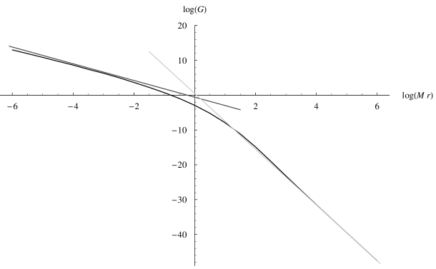
Figure 1: Flow $k=1$, logarithmic plot of the correlator $G(r)=\langle\Theta(x)\Theta(0)\rangle$ (black line) together with both the IR (grey line) and the UV (dark-grey line) behaviours.

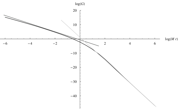
Figure 2: Flow $k=2$, logarithmic plot of the correlator $G(r)=\langle\Theta(x)\Theta(0)\rangle$ (black line) together with both the IR (grey line) and the UV (dark-grey line) behaviours.

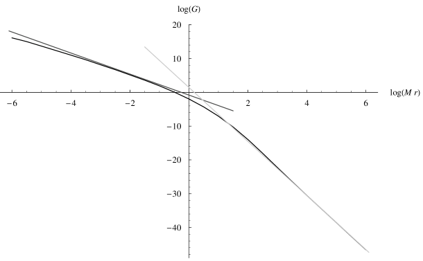
Figure 3: Flow $k=3$, logarithmic plot of the correlator $G(r)=\langle\Theta(x)\Theta(0)\rangle$ (black line) together with both the IR (grey line) and the UV (dark-grey line) behaviours.

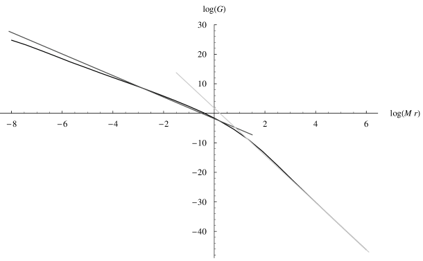
Figure 4: Flow $k=10$, logarithmic plot of the correlator $G(r)=\langle\Theta(x)\Theta(0)\rangle$ (black line) together with both the IR (grey line) and the UV (dark-grey line) behaviours.

References

• [1] M. Karowski and P. Weisz, Nucl. Phys. B139 (1978) 455.
• [2] B. Berg, M. Karowski and P. Weisz, Phys. Rev. D19 (1979) 2477
• [3] F.A. Smirnov, ”Form factors in completely integrable models of Quantum Field theory”, Adv. Series in Math. Phys. 14, World Scientific 1992.
• [4] O.A. Castro-Alvaredo and A. Fring, Phys. Rev. D64 (2001) 085007 [arXiv:hep-th/0010262].
• [5] A.B. Zamolodchikov, JETP Lett. 43 (1986) 730 [Pisma Zh. Eksp. Teor. Fiz. 43 (1986) 565].
• [6] J.L. Cardy, Phys. Rev. Lett. 60 (1988) 2709.
• [7] Al.B. Zamolodchikov, Nucl. Phys. B358 (1991) 524.
• [8] G. Delfino, G. Mussardo and P. Simonetti, Phys.  Rev. D 51 (1995) 6620 [arXiv:hep-th/9410117].
• [9] A.B. Zamolodchikov, Sov. J. Nucl. Phys. 46 (1987) 1090 [Yad. Fiz. 46 (1987) 1819].
• [10] A.W.W. Ludwig and J.L. Cardy, Nucl. Phys. B285 (1987) 687.
• [11] D.A. Kastor, E.J. Martinec and S.H. Shenker, Nucl. Phys. B316 (1989) 590.
• [12] B. Ponsot, “Form factors in the $SS$ model and its RSOS restrictions”, [arXiv:hep-th/0405218].
• [13] V.A. Fateev, Nucl. Phys. B473 (1996) 509.
• [14] C. Crnkovic, G.M. Sotkov and M. Stanishkov, Phys. Lett. B226 (1989) 297.
• [15] P. Goddard, A. Kent and D.I. Olive, Phys.  Lett. B152 (1985) 88.
• [16] A.B.  Zamolodchikov and Al.B.  Zamolodchikov, Nucl. Phys. B379 (1992) 602.
• [17] P. Méjean and F.A. Smirnov, Int. J. Mod. Phys. A12 (1997) 3383 [arXiv:hep-th/9609068].
• [18] S. Coleman, Phys. Rev. D11 (1975) 2088.
• [19] A.B. Zamolodchikov and Al.B. Zamolodchikov, Annals Phys. 120 (1979) 253.
• [20] H. Babujian, A. Fring, M. Karowski and A. Zapletal, Nucl. Phys. B538 (1999) 535 [arXiv:hep-th/9805185].
• [21] H. Babujian and M. Karowski, Nucl. Phys. B620 (2002) 407 [arXiv:hep-th/0105178].
• [22] A. LeClair, Phys.  Lett. B230 (1989) 103, D. Bernard and A. Leclair, Nucl. Phys. B340 (1990) 721, F.A. Smirnov, Int. J. Mod. Phys. A4 (1989) 4213 and Nucl. Phys. B337 (1990) 156,
• [23] N.Yu. Reshetikhin and F.A. Smirnov, Commun. Math.  Phys. 131 (1990) 157.
• [24] A.B. Zamolodchikov, JETP Lett. 46 (1987), 160.
• [25] D. Bernard, Phys.  Lett.  B279 (1992) 78 [arXiv:hep-th/9201006].
• [26] H.E. Boos, V.E. Korepin and F.A. Smirnov, “Connecting lattice and relativistic models via conformal field theory”, [arXiv:math-ph/0311020], to appear in Birkhäuser series ”Progress in Mathematics”.
• [27] B. Ponsot, Phys. Lett. B575 (2003) 131 [arXiv:hep-th/0304240].
• [28] G. Delfino, Phys. Lett. B450 (1999) 196 [arXiv:hep-th/9811215].
• [29] V.A. Fateev, Phys. Lett. B324 (1994) 45.
• [30] P. Grinza and B. Ponsot, ”Form-factors in the massless coset models $su(2)_{k+1}\otimes su(2)_{k}/su(2)_{2k+1}$ Part II”, to appear.
Refer to caption