CERN–PH–TH/2004-217 hep-th/0411032
Splitting Supersymmetry in String Theory

Abstract

We point out that type I string theory in the presence of internal magnetic fields provides a concrete realization of split supersymmetry. To lowest order, gauginos are massless while squarks and sleptons are superheavy. We build such realistic $U(3)\times U(2)\times U(1)$ models on stacks of magnetized D9-branes. Though not unified into a simple group, these theories preserve the successful supersymmetric relation of gauge couplings, as they start out with equal $SU(3)$ and $SU(2)$ couplings and the correct initial $\sin^{2}{\theta_{W}}$ at the compactification scale of $M_{\rm GUT}\simeq 2\times 10^{16}$ GeV, and they have the minimal low-energy particle content of split supersymmetry. We also propose a mechanism in which the gauginos and higgsinos are further protected by a discrete R-symmetry against gravitational corrections, as the gravitino gets an invariant Dirac mass by pairing with a member of a Kaluza-Klein tower of spin-3/2 particles. In addition to the models proposed here, split supersymmetry offers novel strategies for realistic model-building. So, TeV-scale string models previously dismissed because of rapid proton decay, or incorrect $\sin^{2}{\theta_{W}}$, or because there were no unused dimensions into which to dilute the strength of gravity, can now be reconsidered as candidates for realistic split theories with string scale near $M_{\rm GUT}$, as long as the gauginos and higgsinos remain light.

1 Introduction

Some recent developments challenge us to re-examine our preconceived notions of naturalness and our expectations for physics beyond the Standard Model at the LHC. First is the absence of any deviation from the Standard Model suggesting that, if there is new physics at a TeV, it appears to be fine-tuned at the per-cent level and does not comply with our notion of naturalness. Second, and most important, the cosmological constant problem (CCP) presents us with a fine-tuning much more severe than that of the gauge hierarchy problem (GHP). This raises the possibility that the mechanism which solves the CCP may also solve the GHP, and casts some doubts on all the mechanisms proposed so far to address the GHP (technicolor, low-energy supersymmetry (SUSY), low-scale strings, warping, little higgs), since none of them addresses the CCP problem.

One concrete idea addressing the CCP is Weinberg’s anthropic approach [1] which postulated the existence of an enormous “landscape” of vacua, only a small fraction of which have a vacuum energy small enough to allow the formation of galaxies, which provide for a natural (and possibly necessary) habitat for observers such as ourselves. This approach has recently gained momentum because of the realization that string theory may have such a vast landscape of vacua  [2]. Such an environment may drastically change what is a natural or likely theory. To see how this may happen, first recall that the standard measure of fine-tuning in SUSY theories is given by $f_{standard}\sim{m_{H}^{2}\over m_{S}^{2}}$, where $M_{H}\sim 100$ GeV is the Higgs mass and $m_{S}$ is the SUSY-breaking scale. Consider now a neighborhood in the landscape where the density of vacua increases with the scale of SUSY breaking proportional to $m_{S}^{2N}$ [3]. Then, assigning equal a priori probability to each vacuum, the proper new measure of fine-tuning, which takes into account the “entropy” associated with the density of vacua, is $f_{new}\sim{m_{H}^{2}\over m_{S}^{2}}\times m_{S}^{2N}$. For $N>1$, it thus favors large SUSY-breaking scale $m_{S}$.

In such neighborhoods of the landscape low-scale SUSY is disfavored and, if we live in such a neighborhood, the simplest possibility is that we will discover the Standard Model (SM), rather than the supersymmetric Standard Model, at the LHC. This would then account for why we have not seen any evidence for low-energy supersymmetry, at the expense of giving up the two successes of the supersymmetric SM [4]: gauge coupling unification [5] and natural dark-matter (DM) candidate [4, 6]. A more interesting possibility that preserves these successes is that approximate chiral symmetries protect the fermions of the supersymmetric SM down to the TeV scale  [7, 8, 9, 10]. Actually, gauge coupling unification based on extrapolation of low-energy data to high energies is strictly speaking only an indirect indication of light gauginos and higgsinos, rather than of the full super-particle spectrum.

In these theories, the sparticle spectrum is “split” in two: (1) the scalars (squarks and sleptons) that get a mass at the high-scale of supersymmetry breaking $m_{S}$, which can be as large as the grand unification (GUT) scale, and (2) the fermions (gauginos and higgsinos) which are near the electroweak scale and account for both gauge-coupling unification and DM. The only light scalar in this theory is a finely-tuned Higgs. Rather than the boring prediction that the LHC will discover just the Higgs, these theories – called Split Supersymmetry – predict gauginos and higgsinos at a TeV, maintain the successes of the supersymmetric SM, and account for the absence of any evidence for physics beyond the Standard Model, so far.

The main objective of this paper is to build models of split supersymmetry based on string theory. It is clear that split supersymmetry offers novel, previously unavailable, strategies for realistic model-building, and some previously discarded classes of models can now be reconsidered. For example, classes of models of intersecting branes that were studied in the context of low-scale strings [11, 12], and dismissed because of rapid proton decay or the value of the weak mixing angle will now be reconsidered, in section 6, and shown to contain good candidates for realistic theories. Some TeV-scale string models were also abandoned because of the absence of unused dimensions into which to dilute the strength of gravity [13] should be reconsidered as candidates for realistic split theories with string scale near $2\times 10^{16}$ GeV, as long as the gauginos and higgsinos can remain light as a result of an approximate chiral symmetry.

Another objective is to build theories where the successful unification relation is preserved. In split SUSY theories this is not a luxury but an essential ingredient, since unification is a fundamental phenomenological motivation for the “split” spectrum of these theories. This is a strong theoretical constraint, since it limits us to very economical fundamental theories with few relevant parameters in the gauge sector, small threshold corrections, minimal particle content, equal $SU(2)$ and $SU(3)$ couplings as well as the correct normalization of the weak mixing angle at the GUT scale ($\sin^{2}\theta_{W}=3/8$).

Our paper is organized as follows. In Section 2 we discuss the theoretical framework, which is type I string theory with internally magnetized D9 branes. We show that the (tree-level) spectrum of the resulting models is the one required by split supersymmetry. In Section 3, we discuss the conditions that guarantee unification of non-abelian gauge couplings and show that they can be naturally satisfied. In Section 4, we discuss the various mass scales and the supersymmetry breaking in the gravity sector. In Section 5, we propose mechanisms to keep gauginos (and higgsinos) light in the presence of gravity. In Section 6, we study issues of model building and present an explicit example of the SM embedding in the above framework, with realistic particle spectrum, realizing the unification conditions and predicting the correct weak mixing angle $\sin^{2}\theta_{W}=3/8$ at the GUT scale. Finally, in Section 7, we discuss some phenomenological consequences and in particular constraints from gluino cosmology.

2 The framework

We start with type I string theory, or equivalently type IIB with orientifold planes and D-branes. Upon compactification in four dimensions on a Calabi-Yau manifold, one gets ${\cal N}=2$ supersymmetry in the bulk and ${\cal N}=1$ on the branes. Moreover, various fluxes can be turned on, to stabilize part or all of the closed string moduli. We then turn on internal magnetic fields [14, 15], which, in the T-dual picture, amounts to intersecting branes [16, 17]. For generic angles, or equivalently for arbitrary magnetic fields, supersymmetry is spontaneously broken and described by effective D-terms in the four-dimensional (4d) theory [14]. In the weak field limit, $|H|\alpha^{\prime}<1$, the resulting mass shifts are given by:

$$\delta M^{2}=(2k+1)|qH|+2qH\Sigma\qquad;\qquad k=0,1,2,\dots\,,$$ (2.1)

where $H$ is the magnetic field of an abelian gauge symmetry, corresponding to a Cartan generator of the higher dimensional gauge group, on a non-contractible 2-cycle of the internal manifold. $\Sigma$ is the corresponding projection of the spin operator, $k$ is the Landau level and $q=q_{L}+q_{R}$ is the charge of the state, given by the sum of the left and right charges of the endpoints of the associated open string. We recall that the exact string mass formula has the same form as (2.1) with $qH$ replaced by:

$$qH\longrightarrow\theta_{L}+\theta_{R}\qquad;\qquad\theta_{L,R}=\arctan(q_{L,R}H\alpha^{\prime})\,,$$ (2.2)

where $\alpha^{\prime}$ is the string Regge slope. Obviously, the field theory expression (2.1) is reproduced in the weak field limit.

To illustrate the physics, consider an effective six-dimensional (6d) theory compactified on a magnetized “2-cycle”. From the mass formula (2.1), it follows that all charged scalars become massive, since the internal spin $\Sigma$ either vanishes (for six-dimensional scalars), or has eigenvalues $\pm 1$ (for 6d vectors). Actually, one of the two spin-1 helicities becomes tachyonic, reflecting the Nielsen-Olesen instability. This tachyon can be avoided, either when several magnetic fields are turned on in more than one internal 2-cycles [14], or in more realistic models with ${\cal N}=1$ supersymmetry in four dimensions. In the former case, one provides a positive contribution to its mass-squared (see below), while in the latter, one uses an orbifold-type projection which reduces the supersymmetry from its maximal value of the toroidal compactification to ${\cal N}=1$. On the other hand, fermions have four-dimensional (4d) chiral zero modes, since they have internal helicities $\Sigma=\pm 1/2$ and only one of the two leads to a massless mode for $k=0$. Note that neutral states with respect to the magnetized $U(1)$ generator are not affected and form ${\cal N}=1$ supermultiplets. In particular, all gauge bosons of the unbroken gauge group are accompanied by massless gauginos.

In the general case of a magnetic field pointed in several directions of the six-dimensional internal manifold, $H$ and $H\Sigma$ are replaced by ${\rm Tr}JH$ and ${\rm Tr}H\Sigma$, where $J$ is the antisymmetric “identity” matrix with elements $+1(-1)$ above (below) the diagonal and zero everywhere else. For instance, when the internal manifold is a product of three factorized tori $\prod_{I=1}^{3}T^{2}_{(I)}$, one has $H=\sum_{I}H_{I}$ and $H\Sigma=\sum_{I}H_{I}\Sigma_{I}$, where $\Sigma_{I}$ is the projection of the internal helicity along the $I$-th plane. For a ten-dimensional (10d) spinor, its eigenvalues are $\Sigma_{I}=\pm 1/2$, while for a 10d vector $\Sigma_{I}=\pm 1$ in one of the planes $I=I_{0}$ and zero in the other two $(I\neq I_{0})$. Thus, charged higher dimensional scalars become massive, fermions lead to chiral 4d zero modes if all $H_{I}\neq 0$, while the lightest scalars coming from 10d vectors have masses

$$M_{0}^{2}=\left\{\begin{matrix}|qH_{1}|+|qH_{2}|-|qH_{3}|\cr|qH_{1}|-|qH_{2}|+|qH_{3}|\cr-|qH_{1}|+|qH_{2}|+|qH_{3}|\cr\end{matrix}\right.$$ (2.3)

Note that all of them can be made positive definite if all $H_{I}\neq 0$. Moreover, one can easily show that if a scalar mass vanishes, some supersymmetry remains unbroken [15].

The Gauss law for the magnetic flux implies that the fields $H_{i}$ are quantized in terms of the area of the corresponding 2-cycles $A_{i}$:

$$H_{i}={m_{i}\over n_{i}A_{i}}\,,$$ (2.4)

where the integers $m_{i},n_{i}$ correspond to the respective magnetic and electric charges; $m_{i}$ is the quantized flux and $n_{i}$ is the wrapping number of the higher dimensional brane around the corresponding internal 2-cycle. For a rectangular torus of radii $R_{1}$ and $R_{2}$ in the directions $X_{1}$ and $X_{2}$, the area is $A=R_{1}R_{2}$. Open string propagation in magnetic fields has a T-dual representation in terms of D-branes at angles. For instance, starting with a D$p$ brane on a magnetized rectangular torus and applying a T-duality in the direction $X_{2}$, $R_{2}\to\alpha^{\prime}/R_{2}$, leads to a D$(p-1)$ brane wrapped on a direction forming an angle $\theta$ relative to the $X_{1}$ axis, given by the dual of the magnetic field:

$$H\alpha^{\prime}\to\tan\theta={mR_{2}\over nR_{1}}\,.$$ (2.5)

Thus, the integers $m$ and $n$ in (2.4) become the wrapping numbers around the $X_{2}$ and $X_{1}$ directions, respectively.

We consider now several abelian magnetic fields $H_{i}^{a}$ of different Cartan generators $U(1)_{a}$, so that the gauge group is a product of unitary factors $\prod_{a}U(N_{a})$ with $U(N_{a})=SU(N_{a})\times U(1)_{a}$. In an appropriate T-dual representation, it amounts to consider several stacks of D6-branes intersecting in the three internal tori at angles determined by the magnetic fields according to (2.5). An open string with one end on the $a$-th stack has charge $\pm 1$ under the $U(1)_{a}$, depending on its orientation, and is neutral with respect to all others. Using the results described above, the massless spectrum of the theory falls into three sectors [17]:

1. Neutral open strings ending on the same stack, giving rise to ${\cal N}=1$ gauge supermultiplets of gauge bosons and gauginos.

2. Doubled charged open strings from a single stack, with charges $\pm 2$ under the corresponding $U(1)$, giving rise to massless fermions transforming in the antisymmetric or symmetric representation of the associated $SU(N)$ factor. Their bosonic superpartners become massive. For factorized toroidal compactifications $(T^{2})^{3}$, the multiplicities of chiral fermions are given by:

   $${\rm Antisymmetric} : \quad{1\over 2}\left(\prod_{I}2m_{I}^{a}\right)\left(\prod_{J}n_{J}^{a}+1\right)$$

   $${\rm Symmetric} : \quad{1\over 2}\left(\prod_{I}2m_{I}^{a}\right)\left(\prod_{J}n_{J}^{a}-1\right)$$ (2.6)

   where $a$ denotes the D-brane stack, $I$ is the label of the two-torus $T^{2}_{(I)}$, and $m_{I}^{a},n_{I}^{a}$ are the integers entering in the expression of the magnetic field (2.4). For orbifolds or more general Calabi-Yau spaces, the above multiplicities may be further reduced by the corresponding supersymmetry projection down to ${\cal N}=1$.

   In the degenerate case where a magnetic field vanishes, say, along one of the tori ($m_{I}^{a}=0$ for some $I$), there are no chiral fermions in $d=4$ dimensions, but the same formula with the products extending over the other two magnetized tori gives the multiplicities of chiral fermions in $d=6$. In this case, chirality in four dimensions may arise only when the last $T^{2}$ compactification is combined with some additional orbifold-type projection.

3. Open strings stretched between two different brane stacks, with charges $\pm 1$ under each of the corresponding $U(1)$s. They give rise to chiral fermions transforming in the bifundamental representation of the two associated unitary group factors. Their multiplicities, for toroidal compactifications, are given by:

   $$(N_{a},N_{b}) : \prod_{I}(m_{I}^{a}n_{I}^{b}+n_{I}^{a}m_{I}^{b})$$

   $$(N_{a},{\overline{N}}_{b}) : \prod_{I}(m_{I}^{a}n_{I}^{b}-n_{I}^{a}m_{I}^{b})\,.$$ (2.7)

   As in the previous case, when a factor in the products of the above multiplicities vanishes, there are no 4d chiral fermions, but the same formula with the product extending over the other two magnetized tori gives the corresponding multiplicity of chiral fermions in $d=6$.

As mentioned already above, all charged bosons are massive. Massless scalars can appear only when some supersymmetry remains unbroken. In case 2 of doubled charged strings from the same stack, the requirement of massless scalars is equivalent to unbroken supersymmetry on the corresponding brane stack. For toroidal compactifications, using the mass formula (2.3), the condition for the $a$-th stack is

$$\delta H_{a}\equiv\epsilon_{1}H_{1}^{a}+\epsilon_{2}H_{2}^{a}+\epsilon_{3}H_{3}^{a}=0\,,$$ (2.8)

where $H_{I}^{a}$ is the magnetic field of $U(1)_{a}$ on the two-torus $T^{2}_{(I)}$, and $\epsilon_{I}$ are signs $\pm$ with one at least different from the others ($(\epsilon_{1},\epsilon_{2},\epsilon_{3})=(+,+,-)$ or $(+,-,+)$ or $(-,+,+)$). In case 3 of strings ending on two different sets of branes, massless scalars arise when one has unbroken supersymmetry locally, at the intersection. The generalization of the above condition is:

$$\delta H_{ab}\equiv\delta H_{a}-\delta H_{b}=0\,.$$ (2.9)

In the T-dual representation, condition (2.9) involves the relative intersection angles $(\theta_{I}^{a}-\theta_{I}^{b})$, defined as in eq. (2.5).

It is now clear that the above framework leads to models with a tree-level spectrum realizing the idea of split supersymmetry. Embedding the Standard Model (SM) in an appropriate configuration of D-brane stacks, one obtains tree-level massless gauginos while all scalar superpartners of quarks and leptons typically get masses at the scale of the magnetic fields, whose magnitude is set by the compactification scale of the corresponding internal space.

On the other hand, the condition to obtain a (tree-level) massless Higgs in the spectrum implies that supersymmetry remains unbroken in the Higgs sector, leading to a pair of massless higgsinos, as required by anomaly cancellation. Note that since the Higgs doublet has the same quantum numbers with leptons, it is likely that lepton doublets have the same open string origin as the Higgs scalar, and thus, left-handed sleptons are also massless at the tree-level.

3 Gauge coupling unification

On general grounds, there are two conditions to obtain unification of Standard Model gauge interactions, consistently with extrapolation of gauge couplings from low-energy data using the minimal supersymmetric SM spectrum. (i) Equality of the $SU(3)$ color and weak $SU(2)$ non-abelian gauge couplings and (ii) the correct prediction for the weak mixing angle $\sin^{2}\theta_{W}=3/8$ at the grand unification (GUT) scale. On the other hand, a generic D-brane model using several stacks, as described in the framework of the previous section, does not satisfy either of the two conditions. Indeed, this framework was developed in connection to the idea of low-scale strings [11, 12], where the concept of unification is radically different from conventional GUTs. In this section, we study precisely the general requirements for satisfying the first of the above two conditions, namely natural unification of non-abelian gauge couplings. The second condition is more involved and model dependent, since it is related with the particular hypercharge embedding and will be discussed in section 6.

The four-dimensional non-abelian gauge coupling $\alpha_{N_{a}}$ of the $a$-th brane stack is given by:

$${1\over\alpha_{N_{a}}}={V^{a}\over g_{s}}\prod_{I}|n_{I}^{a}|\sqrt{1+(H_{I}^{a}\alpha^{\prime})^{2}}\,,$$ (3.1)

where $g_{s}$ is the string coupling and $V^{a}$ the compactification volume in string units of the internal space of the $a$-th brane stack. The presence of the wrapping numbers $|n_{I}^{a}|$ can be understood from the fact that $|n_{I}^{a}|V^{a}_{I}$ is the effective area of the 2-torus $T^{2}_{(I)}$ wrapped $n_{I}^{a}$ times by the brane, and $V^{a}=\prod_{I}V^{a}_{I}$. The additional factor in the square root follows from the non-linear Dirac-Born-Infeld (DBI) action of the abelian gauge field, $\sqrt{\det(\delta_{ij}+F_{ij}\alpha^{\prime})}$, which in the case of two dimensions with $F_{ij}=\epsilon_{ij}H$, it is reduced to $\sqrt{1+(H\alpha^{\prime})^{2}}$. Obviously, the expression (3.1) holds at the compactification scale, since above it gauge couplings receive important corrections and become higher dimensional. Finally, the gauge couplings of the associated abelian factors, in our convention of $U(1)$ charges, are given by

$$\alpha_{{}_{U(1)_{a}}}={\alpha_{N_{a}}\over{2N_{a}}}\,.$$ (3.2)

Here, non-abelian generators are normalized according to ${\rm Tr}T^{a}T^{b}=\delta^{ab}/2$.

From equation (3.1), it follows that unification of non-abelian gauge couplings holds if (i) $V^{a}$ and (ii) $\prod_{I}|n_{I}^{a}|$ are independent of $a$, while (iii) the magnetic fields are either $a$-independent as well, or they are much smaller than the string scale.

• The first condition (i) is automatically satisfied for D9-branes, since then $V^{a}=V$, the total volume of the six dimensional internal manifold.

• The second condition (ii) is satisfied for a large class of models with $|n_{I}^{a}|=1$, which is the point particle field theoretic value of Dirac quantization for magnetic fields (no multiple brane wrapping). Actually, this value follows also from eq. (2.6), by requiring the absence of chiral fermions transforming in the symmetric representations of the non-abelian groups, i.e. no chiral $SU(3)$ color sextets and no weak $SU(2)$ triplets.

• The third condition (iii) of weak magnetic fields is more quantitative. Allowing for $1\%$ error in the unification condition at high scale, one should have $H_{I}^{a}\alpha^{\prime}\mathrel{\lower 2.5pt\vbox{\hbox{$<$}\hbox{$\sim$}}}0.1$. From the quantization condition (2.4), this implies that the volume $V\mathrel{\lower 2.5pt\vbox{\hbox{$>$}\hbox{$\sim$}}}10^{3}$ for three magnetized tori, which is rather high to keep the theory weakly coupled above the compactification scale. Indeed, eq. (3.1) gives a string coupling $g_{s}$ of order ${\cal O}(10)$ for gauge couplings $\alpha_{N_{a}}\simeq 1/25$ at the unification scale. On the other hand, for one or two magnetized tori one obtains $V\mathrel{\lower 2.5pt\vbox{\hbox{$>$}\hbox{$\sim$}}}10-10^{2}$, which is compatible with a string weak coupling regime $(g_{s}\sim 0.1-1)$. Of course this discussion should be taken with caution, because there is an uncertainty in the relation of $g_{s}$ with the string loop expansion parameter. Here, we were conservative and defined it as in a 4d gauge theory. In a 10d theory however, there may be additional powers of $2\pi$ which would improve significantly perturbativity [18].

  Actually, the condition of weak magnetic fields can be partly relaxed in some direction, by requiring the absence of chiral antiquark doublets in the spectrum. Indeed eq. (2.7), for open strings stretched between the strong $SU(3)$ and weak $SU(2)$ interactions brane stacks, implies the vanishing of one of the factors in the product. This leads to the equality of the ratio $m_{I}^{a}/n_{I}^{a}$ for the two stacks and for some $I$, and thus, to the equality of the two corresponding magnetic fields via eq. (2.4). As a result, the condition of perturbativity is weakened and becomes possible even in the case of three factorized magnetized tori.

Note that in the T-dual representation of intersecting D6-branes, the unification conditions discussed above appear less natural. In the expression (3.1) of gauge couplings, the numerator ($V^{a}$ times the product) is replaced by the volume of the 3-cycle around which the D6 brane wraps. For instance, in the case of three factorized rectangular tori of radii $R^{I}_{1}$ and $R^{I}_{2}$ in string units, it is given by $\prod_{I}\sqrt{(n_{I}^{a}R_{1}^{I})^{2}+(m_{I}^{a}R_{2}^{I})^{2}}$. The same unification conditions then hold in this context, with the requirement of weak magnetic field replaced by the requirement of small angle, which is equivalent to the inequality $R_{2}^{I}<<R_{1}^{I}$ (see eq. (2.5)).

The above analysis concerns mainly the QCD and $SU(2)_{L}$ gauge couplings $\alpha_{3}$ and $\alpha_{2}$. The case of hypercharge is more subtle since it can be in general a linear combination of several $U(1)$s coming from different brane stacks. In section 6, for the purpose of illustration, we present an explicit example with the correct prediction of the weak mixing angle. It is based on a minimal Standard Model embedding in three brane stacks with the hypercharge being a linear combination of two abelian factors. This provides an existence proof that can be generalized in different constructions. We notice for instance that in a class of supersymmetric models with four brane stacks, the equality of the two non-abelian couplings $\alpha_{2}=\alpha_{3}$ implies the value $3/8$ for $\sin^{2}\theta_{W}$ at the unification scale [19].

4 Mass scales and supersymmetry breaking

The supersymmetry breaking scale $m_{\rm S}$ on the brane stacks is given by the lightest charged scalar masses (2.3), or equivalently by $\delta H_{a}=\sum_{I}\epsilon_{I}H_{I}^{a}$ of eq. (2.8), in the weak field limit. In the case of strong magnetic fields, of order of the string scale, $H_{I}^{a}$ should be replaced by the angles $\theta_{I}^{a}$ according to eqs. (2.2) and (2.5). For magnetic fields in more than one internal planes, $m_{\rm S}$ can therefore be smaller than their magnitude, and consequently from the corresponding compactification scales (2.4). Similarly, on brane intersections, the supersymmetry breaking scale is given by the differences $\delta H_{ab}$ of eq. (2.9), and thus, can be again smaller than $H_{I}^{a}$ and the compactification scales.

Let us now discuss the various mass scales. To preserve gauge coupling unification, the (non-gravitational part of the) theory must remain 4-dimensional up to the unification scale. So the compactification scale (actually the smallest, if there are several) must be no smaller than the unification energy, $M_{\rm GUT}\simeq 10^{16}$ GeV, and we will take them to be of the same order. Above the compactification scale, gauge interactions acquire a higher dimensional behavior. So, to keep the theory weakly coupled, the string scale $M_{s}\equiv{\alpha^{\prime}}^{-1/2}$ should be close to the compactification scale and therefore to $M_{\rm GUT}$. Moreover, as we discussed in the previous section, to ensure that corrections to the unification of gauge couplings are within 1%, the magnetic fields should be weak. It follows that the string scale should be roughly a factor of 3 higher than the compactification scale,

$$M_{s}\mathrel{\lower 2.5pt\vbox{\hbox{$>$}\hbox{$\sim$}}}3\,M_{\rm GUT}\,.$$ (4.1)

On the other hand, as we pointed out above, $m_{\rm S}$ can be lower than $M_{\rm GUT}$. Although much lower values require an apparent fine tuning of radii, such a tuning is technically natural since the supersymmetric point $m_{\rm S}=0$ is radiatively stable. One can therefore treat $m_{\rm S}\sim|\delta H|^{1/2}$ as free parameter and drop for simplicity the brane stacks dependent index in $\delta H$.

All scalar masses are of order $|\delta H|^{1/2}$ except for those coming from supersymmetric sectors, which are vanishing to lowest order, such as the Higgs and possibly the slepton doublets. The latter are expected to acquire masses from one loop corrections, proportional to $|\delta H|^{1/2}$ but suppressed by a loop factor. Note that off diagonal elements of the $2\times 2$ Higgs mass matrix, usually denoted by $B\mu$, should also be generated at the same order as the diagonal elements, in the absence of a Peccei-Quinn (PQ) symmetry. For high $\delta H$, a fine tuning between $B\mu$ and the diagonal elements is then required to ensure a light higgs.

It remains to discuss the corrections to gaugino and higgsino masses, $m_{1/2}$ and $\mu$, which are vanishing at the tree-level. In the absence of gravity, they are both protected by an R-symmetry. Actually, higgsino masses are protected in addition by a PQ symmetry which must be broken in order to generate a $B\mu$ mixing term in the Higgs mass matrix, as we argued above. Then, a $\mu$-term can be generated via $B\mu$, or directly using the PQ symmetry breaking, if R-symmetry is broken. Indeed, R-symmetry is in general broken in the gravitational sector by the gravitino mass $m_{3/2}$ and thus, in the presence of gravity, $m_{1/2}$ and $\mu$ are not anymore protected.

Thus, the study of fermion masses requires some knowledge of supersymmetry breaking in the gravity sector, which has been ignored up to now. A related issue is the cancellation of the cosmological constant between brane and bulk contributions, in order to maintain the flat space background. The brane contribution comes from the supersymmetry breaking due to the magnetic field and scales as $(\delta H)^{p}$, in string units, where the power $p$ depends on the number ${\cal N}$ of bulk supersymmetries broken by $\delta H$. For the maximal value of ${\cal N}=4$ it was found that $p=3$ [14], while for ${\cal N}=1$ we expect that $p=1$, or more precisely $(\delta H)H$ from the form of the DBI action (3.1).

The vanishing of the vacuum energy implies that an additional source of supersymmetry breaking should probably be introduced in the closed string sector (bulk). The corresponding dominant bulk contribution to the cosmological constant is proportional in general to $m_{3/2}^{2}\Lambda^{2}$, with $\Lambda$ the ultraviolet (UV) cutoff. Combining the brane and bulk contributions, one obtains

$$m_{3/2}\sim{|H|^{1/2}\over\Lambda}\times|\delta H|^{1/2}\,.$$ (4.2)

Thus, for $\Lambda\simeq M_{s}$ the gravitino mass is in general of the same order as the scalar masses, while for $\Lambda\simeq M_{P}$, the 4d Planck mass, it is about three orders of magnitude lower.

In the following, we will consider for concreteness a source of bulk supersymmetry breaking via Scherk-Schwarz (SS)  [20] boundary conditions along a “gravitational” interval $S^{1}/Z_{2}$ of length $\pi R$ [21]. This interval can be identified either with the eleventh dimension of M-theory [22], or with some internal orientifold direction of type I string theory, transverse to all “observable” brane stacks where the Standard Model is localized [23]. The gravitino mass is then given by:

$$m_{3/2}={\omega\over R}\,,$$ (4.3)

where $\omega\in[0,1]$ is the parameter of the SS deformation. It originates from the boundary conditions of the five dimensional fields which are periodic up to a phase of a symmetry transformation [20]. The latter can be parametrized as $e^{2i\pi\omega/R}$ and corresponds to a discrete rotation in the internal compactified space, in order to give a mass to the gravitino. Therefore, $\omega$ is quantized and equals $1/N$ for $Z_{N}$.

Using now the usual relations that express the 4d Planck mass $M_{P}$ and the gauge coupling at the unification scale $\alpha_{G}$ in terms of the string parameters (scale, coupling and compactification sizes), one finds upon eliminating the string coupling [21, 12]:

$$R^{-1}={2\over\alpha_{G}^{2}}{M_{s}^{3}\over M_{P}^{2}}V^{-1}\,,$$ (4.4)

where $V$ is the internal compactification volume (in string units) of all SM branes. Substituting the values discussed above for $M_{s}$ and $V$, one finds $R^{-1}\simeq{\cal O}(10^{13}-10^{14})$ GeV. Following our previous discussion on the cancellation of vacuum energy, when combining the SS bulk supersymmetry breaking with the brane magnetic fields, one expects that $|\delta H|^{1/2}$ should also be of the same order $10^{13}$ GeV. On the other hand, because of the uncertainty in the value of the relevant UV cutoff in eq. (4.2), the scalar masses could be either significantly higher, of order of the unification scale, or lower, of order of $10^{10}$ GeV for $\Lambda\simeq R^{-1}\simeq m_{3/2}$, as was argued in the context of SS compactifications [24]. Thus, in section 7, we will study the phenomenology of the whole range of scalar masses $m_{S}\simeq 10^{10}-10^{16}$ GeV.

5 Light gaugino masses

In the presence of R-symmetry, gluinos can only get a Dirac mass by pairing up with other color octet fermions, which spoils gauge coupling unification. So, gluinos must either be massless, which is phenomenologically strongly disfavored, or get an R-breaking Majorana mass. The latter requires a source for R-breaking, and would also permit, in combination with PQ breaking, the generation of higgsino masses.

One possible source of R-symmetry breaking is the Majorana mass for the gravitino. Such a mass is always present, as a result of canceling the tree-level cosmological constant, in theories where there is an energy regime in which 4d supergravity holds. A second possibility is that there is no such an energy regime, the gravitino gets an R-preserving Dirac mass by pairing up with another spin-3/2 fermion, and R-symmetry is broken spontaneously by a dynamical condensate. In this section, we will consider both possibilities, beginning with the first.

The first possibility has already been studied in some detail in the effective field theory [25, 7, 10]. Once R-symmetry, as well as supersymmetry, is broken through the Majorana gravitino mass, the gauginos can get a mass in a number of ways. One is anomaly mediation [26], whose leading contribution can be adequately suppressed to allow for light gauginos in the presence of heavy gravitinos [25, 10].

In string theory, gaugino masses mediated from closed string radiative corrections have been studied recently and shown to be generated at lowest order by string diagrams of “one and a half” loop (“genus” 3/2) [27]. They contain for instance one handle and one boundary. It turns out that for generic compactifications and supersymmetry breaking mechanism, the resulting gaugino masses are proportional to the gravitino mass for small $m_{3/2}$ compared to the string scale: $m_{1/2}\sim\alpha^{2}m_{3/2}$ with $\alpha$ the corresponding gauge coupling. Apart from the power of gauge coupling, this result is similar to the contribution of anomaly mediation [28].

Suppression of the anomaly mediation contribution in radiative corrections may arise as follows. A generic contribution to the gaugino mass involves gravity and gauge loops and should contain a gravitino mass insertion that brings one power of $m_{3/2}$. From an effective field theory analysis, one expects that the dominant contribution of each gravity loop is proportional to $\Lambda^{2}/M_{P}^{2}$, with $\Lambda$ the UV cutoff, since each gravitational vertex brings an inverse power of Planck mass $M_{P}$ and the loop is quadratically divergent. Moreover, gauge loops do not modify this power counting. If the UV cutoff is set up by the Planck scale, $m_{1/2}$ would be proportional to $m_{3/2}$. However, in special models with supersymmetry breaking via Scherk-Schwarz compactifications, one expects a UV cutoff set by the compactification scale [24], in which case the dominant contribution comes from one gravitational loop, leading to $m_{1/2}\propto m_{3/2}^{3}/M_{P}^{2}$ [25, 7]. Thus, gauginos (and higgsinos) become light around the TeV scale, for instance when $m_{3/2}\sim|\delta H|^{1/2}\simeq 10^{13-14}$ GeV as we argued above.

On the other hand, in the string theory analysis, it was found that for orbifold compactifications the corrections to $m_{1/2}$ are exponentially suppressed for small gravitino mass at the lowest non-trivial order of “genus” 3/2 [27]. This is an indication that these models are indeed examples of quantum gravitational suppressed anomaly mediation, which may be checked by going to the next non-trivial order.

We now present a different mechanism to protect gaugino masses in the presence of gravity, based on symmetry. It involves theories in which there is no 4d supergravity energy regime, the gravitino gets an R-preserving Dirac mass by pairing up with another spin-3/2 fermion, and therefore does not feed a mass to the gluino. The breaking of R-symmetry, which is necessary to give masses to the gluinos and higgsinos, can subsequently occur via a dynamical condensate.

We begin from the observation that the lowest order perturbative correction to $m_{1/2}$ is exactly vanishing for the case of $Z_{2}$ SS deformation with $\omega=1/2$ (see eq. (4.3)) [29, 27]. Indeed, here we will argue that the usual SS compactification with a $Z_{2}$ shift in a direction transverse to the brane leaves unbroken a generalized R-type symmetry, which guarantees the vanishing of gaugino masses in the full theory. We will use the effective field theory description of the whole tower of Kaluza-Klein (KK) excitations for a generic SS compactification on a circle of radius $R$ [30]. A massless five-dimensional (5d) spinor $\psi$, with SS boundary conditions twisted by the phase $e^{2i\pi\omega/R}$ around the circle, gives rise in four dimensions to the following $2\times 2$ mass matrix for each pair of KK levels $|n>$ and $|-n>$ :

$${1\over R}\left(\psi^{L}_{n}\ \psi^{R}_{n}\right)\left(\begin{matrix}\omega&n\cr n&\omega\cr\end{matrix}\right)\left(\begin{matrix}\psi^{L}_{n}\cr\psi^{R}_{n}\cr\end{matrix}\right)\quad;\quad n=0,1,2\dots\,,$$ (5.1)

where $\psi^{L,R}_{n}$ is the left (L) and right (R) component of the $n$-th KK excitation of the fermion. The diagonal element $\omega$ arises from the SS deformation. The eigenvalues of the above mass matrix are $(\omega\pm n)/R$, reproducing the familiar shift of the KK number.

Here, we consider a SS direction which is transverse to the brane stack, so that gauginos are not affected and supersymmetry remains unbroken on the branes in the presence of the SS deformation. The only source of supersymmetry breaking on the branes comes from the magnetic fields on their world volume, which give masses to all charged scalars, as we described previously. Thus, in this case, the SS direction is not a circle but an interval $S^{1}/Z_{2}$, with $Z_{2}$ being the inversion of the extra coordinate. Its action on the KK spectrum consists of sending $|n>\to|-n>$, while at the same time acts on 4d fermion chiralities: left-hand components are invariant and right-handed change sign. As a result, the $Z_{2}$ projection on the KK spectrum of a 5d spinor keeps the left-handed symmetric and right-handed antisymmetric combinations of states $(|n>_{{}_{L}}+|-n>_{{}_{L}})/\sqrt{2}$ and $(|n>_{{}_{R}}-|-n>_{{}_{R}})/\sqrt{2}$, having cosine and sine wave functions, respectively. Keeping the same notation $\psi^{L}_{n}$ and $\psi^{R}_{n}$ for these $Z_{2}$ invariant combinations, the fermion mass terms can be easily deduced from the expression (5.1) and take the form:

$${\omega\over R}\psi^{L}_{0}\psi^{L}_{0}+{1\over R}\sum_{n\geq 1}\left(\psi^{L}_{n}\ \psi^{R}_{n}\right)\left(\begin{matrix}\omega&n\cr n&\omega\cr\end{matrix}\right)\left(\begin{matrix}\psi^{L}_{n}\cr\psi^{R}_{n}\cr\end{matrix}\right)\,.$$ (5.2)

For a generic SS deformation, corresponding for instance to a $Z_{N}$ shift with $\omega=1/N$ and $N>2$, a simple inspection of eq. (5.2) shows that there is a tower of Majorana masses for the gravitino KK modes, that break the R-symmetry of global supersymmetry. Thus, gauginos are expected to acquire masses through gravitational radiative corrections. Moreover, despite the quantization of $\omega$, one can define three energy regimes in the gravity sector. A low-energy 4d non-supersymmetric region below the lightest KK gravitino mass $\omega/R$, a 5d supergravity region at energies higher than the compactification scale $E>>1/R$, and an intermediate regime at energies $\omega/R<E<1/R$, where one can define a 4d ${\cal N}=1$ spontaneously broken supergravity. The latter can be obtained by integrating out all heavier KK excitations with $n>1$ and describes the physics of the gravitino “zero mode” $n=0$.

This general picture breaks down in the $Z_{2}$ case $\omega=1/2$, due to a new pairing that arises in the KK spectrum. The “zero mode” becomes degenerate with the lightest eigenstate of the $2\times 2$ mixing matrix for the first KK excitation $n=1$, with mass eigenvalue $1/2R$. This degeneracy continues similarly to all KK levels; the heaviest eigenstate at level $n$ with mass eigenvalue $(n+1/2)/R$, becomes degenerate with the lightest eigenstate at level $n+1$. Thus, all masses can be rewritten in a Dirac type form and one can define a new unbroken R-symmetry that keeps gauginos on the transverse branes massless. Note also that in this case, there is no intermediate energy regime where one can define a 4d ${\cal N}=1$ supergravity, since after the SS deformation, the 4d gravitino zero mode is degenerate with another state coming from its $n=1$ KK excitation. Including this extra spin-3/2 state in the effective theory, one should also include its degenerate $n=1$ companion at the symmetric phase, which however, after the SS deformation, becomes degenerate with the lightest eigenstate from the next level $n=2$, and so on. In the effective supergravity, one should therefore include the whole KK tower and the intermediate energy regime is lost.

The low-energy 4d non-supersymmetric region without any gravitino mode has obviously a chiral symmetry associated to the massless gauginos. On the other hand, in order to describe the generalized R-symmetry in the presence of gravity, one has to go directly to the high energy 5d regime with the whole KK gravitino tower. This phenomenon provides the first example of massive supergravity coupled to an exact supersymmetric gauge sector (but non-supersymmetric chiral matter) that survives in the quantum theory. As we mentioned earlier, the R-symmetry can be broken spontaneously by appropriate dynamics within the effective field theory at much lower energies and generate gaugino and higgsino masses close to the electroweak scale, preserving the unification of gauge couplings. In this case, the corresponding breaking scale is an extra parameter that requires separate dynamics.

6 Model building

In this section, we present an explicit Standard Model embedding, in a minimal set of three brane stacks which has a realistic particle content, satisfies the conditions of unification of strong and weak interactions and predicts the correct weak angle $\sin^{2}\theta_{W}=3/8$ at the unification scale. This model illustrates our general framework and provides an explicit example where several problems can be addressed and many general phenomenological consequences can be discussed.

Model building with intersecting branes has been extensively studied in the recent literature, mainly in the context of low-scale string models [11, 12] (see for example ref. [13] and references therein). According to the general analysis of ref. [31], the SM embedding requires usually four stacks of branes, the color $U(3)$, the weak $U(2)$, together with two abelian ones. The hypercharge is in general a linear combination of the four $U(1)$s, while the remaining three orthogonal combinations are usually broken by anomalies to their global counterparts corresponding to the baryon and lepton numbers and a Peccei-Quinn symmetry. Moreover, the value of the weak angle when $\alpha_{3}=\alpha_{2}$ is in general different from $3/8$, which in any case is not a desired value when the string scale is at low energies. Here, we will focus on a particular model that was dropped from the analysis of refs. [31] because, although minimal and very economic, it was not appropriate for low string scale. Its two main defects were the value of the weak angle and the absence of baryon number as a symmetry to guarantee proton stability.

The model requires three stacks of branes giving rise to $U(3)\times U(2)\times U(1)$ gauge group. For completeness, below we will make a general study of SM embedding in three brane stacks [32]. The quark and lepton doublets ($Q$ and $L$) correspond to open strings stretched between the weak and the color or $U(1)$ branes, respectively. On the other hand, the $u^{c}$ and $d^{c}$ antiquarks can come from strings that are either stretched between the color and $U(1)$ branes, or that have both ends on the color branes and transform in the antisymmetric representation of $U(3)$ (which is an anti-triplet). There are therefore three possible models, depending on whether it is the $u^{c}$ (model A), or the $d^{c}$ (model B), or none of them (model C), the state coming from the antisymmetric representation of color branes. It follows that the antilepton $l^{c}$ comes in a similar way from open strings with both ends either on the weak brane stack and transforming in the antisymmetric representation of $U(2)$ which is an $SU(2)$ singlet (in model A), or on the abelian brane and transforming in the “symmetric” representation of $U(1)$ (in models B and C). The three models are presented pictorially in Figure 1.

      

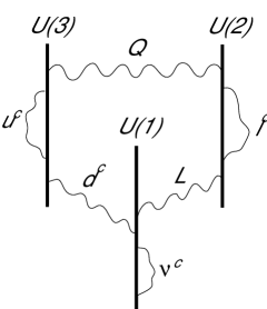
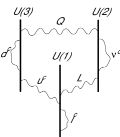
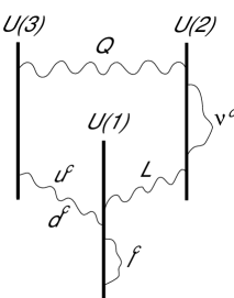
Figure 1: Pictorial representation of models $A$, $B$ and $C$.

Thus, the members of a family of quarks and leptons have the following quantum numbers:

$${\rm Model\ A}\qquad\qquad\quad\quad{\rm Model\ B}\qquad\qquad\quad\ {\rm Model\ C}$$

$$\!\!\!\!\!\!\!\!Q ({\bf 3},{\bf 2};1,1,0)_{1/6}\quad\quad\quad\ ({\bf 3},{\bf 2};1,\varepsilon_{Q},0)_{1/6}\qquad\,({\bf 3},{\bf 2};1,\varepsilon_{Q},0)_{1/6}$$

$$\!\!\!\!\!\!\!\!u^{c} (\bar{\bf 3},{\bf 1};2,0,0)_{-2/3}\quad\quad\ \ \,(\bar{\bf 3},{\bf 1};-1,0,1)_{-2/3}\quad\ (\bar{\bf 3},{\bf 1};-1,0,1)_{-2/3}$$

$$\!\!\!\!\!\!\!\!d^{c} (\bar{\bf 3},{\bf 1};-1,0,\varepsilon_{d})_{1/3}\qquad\,(\bar{\bf 3},{\bf 1};2,0,0)_{1/3}\qquad\ \ \,(\bar{\bf 3},{\bf 1};-1,0,-1)_{1/3}$$ (6.1)

$$\!\!\!\!\!\!\!\!L ({\bf 1},{\bf 2};0,-1,\varepsilon_{L})_{-1/2}\quad\ \,({\bf 1},{\bf 2};0,\varepsilon_{L},1)_{-1/2}\quad\ \ \,({\bf 1},{\bf 2};0,\varepsilon_{L},1)_{-1/2}$$

$$\!\!\!\!\!\!\!\!l^{c} ({\bf 1},{\bf 1};0,2,0)_{1}\qquad\quad\quad\,({\bf 1},{\bf 1};0,0,-2)_{1}\qquad\ \ ({\bf 1},{\bf 1};0,0,-2)_{1}$$

$$\!\!\!\!\!\!\!\!\nu^{c} ({\bf 1},{\bf 1};0,0,2\varepsilon_{\nu})_{0}\qquad\quad\ ({\bf 1},{\bf 1};0,2\varepsilon_{\nu},0)_{0}\qquad\ \,({\bf 1},{\bf 1};0,2\varepsilon_{\nu},0)_{0}$$

where the last three digits after the semi-column in the brackets are the charges under the three abelian factors $U(1)_{3}\times U(1)_{2}\times U(1)$, that we will call $Q_{3}$, $Q_{2}$ and $Q_{1}$ in the following, while the subscripts denote the corresponding hypercharges. The various sign ambiguities $\varepsilon_{i}=\pm 1$ are due to the fact that the corresponding abelian factor does not participate in the hypercharge combination (see below). In the last line, we also give the quantum numbers of a possible right-handed neutrino in each of the three models. These are in fact all possible ways of embedding the SM spectrum in three sets of branes.

The value of the weak angle can be easily computed from the hypercharge combination:

$$Y=\sum_{i}c_{i}Q_{i}\quad\Rightarrow\quad\sin^{2}\theta_{W}={1\over 1+4c_{2}^{2}+2c_{1}^{2}\alpha_{2}/\alpha_{1}+6c_{3}^{2}\alpha_{2}/\alpha_{3}}\,,$$ (6.2)

where $\alpha_{i}$ are the non-abelian couplings and the numerical coefficients are due to our normalization of $U(1)$ charges according to eq. (3.2). In our models, the hypercharge combination is:

$${\rm Model\ A}\quad\ : \quad Y=-{1\over 3}Q_{3}+{1\over 2}Q_{2}$$ (6.3)

$${\rm Model\ B,C} : \quad Y=\ \ \,{1\over 6}Q_{3}-{1\over 2}Q_{1}$$

leading to the following expressions for the weak angle:

$${\rm Model\ A}\quad\ : \quad\sin^{2}\theta_{W}={1\over 2+2\alpha_{2}/3\alpha_{3}}={3\over 8}\,{\bigg{|}}_{\alpha_{{}_{2}}=\alpha_{{}_{3}}}$$ (6.4)

$${\rm Model\ B,C} : \quad\sin^{2}\theta_{W}={1\over 1+\alpha_{2}/2\alpha_{1}+\alpha_{2}/6\alpha_{3}}={6\over 7+3\alpha_{2}/\alpha_{1}}\,{\bigg{|}}_{\alpha_{{}_{2}}=\alpha_{{}_{3}}}$$

In the second part of the above equalities, we used the unification relation $\alpha_{2}=\alpha_{3}$, that can be naturally imposed as described in section 3. Indeed, it follows by requiring the absence of chiral fermions that transform in the symmetric representation of $SU(3)$ and $SU(2)$ and the magnetic fields to be roughly an order of magnitude smaller than the string scale. The last condition can be partly relaxed in model A from the requirement of absence of chiral quark “anti”-doublets in the spectrum. Notice that such states have wrong hypercharge, since their $Q_{2}$ charge is opposite from quark doublets in eq. (6.3). This cannot be used in models B and C because $Q_{2}$ does not participate in the hypercharge combination, and thus, doublets and anti-doublets are indistinguishable. In any case, in these models the unification of the two non-abelian couplings is not sufficient to predict the weak angle and further conditions are needed for the $U(1)$ coupling $\alpha_{1}$. Such an analysis goes beyond the scope of this paper, which is to describe the general framework and present a simple example. Indeed, model A admits natural gauge coupling unification of strong and weak interactions, realizing the conditions we described in section 3, and predicts the correct value for $\sin^{2}\theta_{W}=3/8$ at the unification scale $M_{\rm GUT}$.

The spectrum (6.1) can be easily implemented with a Higgs sector, since the Higgs field $H$ has the same quantum numbers as the lepton doublet or its complex conjugate:

$${\rm Model\ A}\qquad\qquad\quad\quad{\rm Model\ B,C}$$

$$\!\!\!\!\!\!\!\!H\ ({\bf 1},{\bf 2};0,-1,\varepsilon_{H})_{-1/2}\quad\ ({\bf 1},{\bf 2};0,\varepsilon_{H},1)_{-1/2}$$ (6.5)

$$\!\!\!\!\!\!\!\!H^{\prime} ({\bf 1},{\bf 2};0,1,\varepsilon_{H^{\prime}})_{1/2}\qquad\ \,({\bf 1},{\bf 2};0,\varepsilon_{H^{\prime}},-1)_{1/2}$$

Actually, as explained in the general framework of section 2, the Higgs sector should be locally supersymmetric, so that the Higgs scalars are massless at the tree level, and thus $H$ and $H^{\prime}$ correspond to two Higgs chiral supermultiplets.

Besides the hypercharge combination, there are two additional $U(1)$s. It is easy to check that one of the two can be identified with $B-L$. For instance, in model A choosing the signs $\varepsilon_{d}=\varepsilon_{L}=-\varepsilon_{\nu}=-\varepsilon_{H}=\varepsilon_{H^{\prime}}$, it is given by:

$$B-L=-{1\over 6}Q_{3}+{1\over 2}Q_{2}-{\varepsilon_{d}\over 2}Q_{1}\,.$$ (6.6)

The other $U(1)$ corresponds to a Peccei-Quinn (PQ) type symmetry. $B-L$ can be broken by a vacuum expectation value (VEV) of a SM singlet field of the type of $\nu^{c}$, at a high scale. In any case, this model has no baryon number conservation and thus proton is unstable by dimension six effective operators suppressed by the string scale.

The second $U(1)$ combination of PQ type is anomalous. The corresponding gauge field should become massive via the Green-Schwarz mechanism, by absorbing an axion from the Ramond-Ramond (RR) closed string sector [33]. Usually, its global counterpart survives and remains unbroken in perturbation theory at the orbifold point [34]. To avoid the presence of an electroweak axion, one should either move away from this point, or find some appropriate extension of the model which allows to break PQ by a scalar VEV at a high scale. On the other hand, in the presence of magnetic fields, it was noticed that the RR axions involved in the anomaly cancellation come from the untwisted orbifold sector [15]. In this case, the global symmetry will be in general broken at the scale of the anomalous $U(1)$ mass, as in heterotic string models. As a result, the axion becomes invisible and no PQ symmetry should survive at low energies.

7 Constraints from Gluino Cosmology

The most distinctive signature of split SUSY, decisively differentiating it from the usual supersymmetric SM, is the long-lived gluino, which is the smoking gun of this framework. Because the scale of supersymmetry breaking is high, the squarks are heavy and the lifetime for the gluino to decay into a quark, antiquark and LSP – which is mediated by virtual squark exchange – is:

$$\tau=3\times 10^{-2}{\rm sec}\Big{(}\frac{m_{S}}{10^{9}\,{\rm GeV}}\Big{)}^{4}\Big{(}\frac{1\,{\rm TeV}}{m_{\tilde{g}}}\Big{)}^{5},$$ (7.1)

where $m_{S}$ is the squark mass and $m_{\tilde{g}}$ the gluino mass. We have included a QCD enhancement factor of $\sim 10$ in the rate, and another factor $\sim 10$ for the number of decay channels. The longevity of the gluino can lead to a host of interesting signatures at the LHC such as displaced vertices, intermittent tracks, late decaying gluinos captured near the detector etc., which have been discussed in refs. [7, 8, 9, 10]. These signatures depend on the lifetime, which in turn depends sensitively, through the above equation, on the gluino mass and the squark mass $m_{S}\sim\sqrt{\delta H}$. These quantities are constrained by cosmological considerations, to which we turn next.

The most natural value for the squark mass, one that does not require tuning the ratio $\delta H/H$ to be small, is $m_{S}\sim\sqrt{\delta H}\sim M_{GUT}\sim 10^{16}$ GeV. For this value of $m_{S}$, and for $m_{\tilde{g}}\sim 1$ TeV, the gluino lifetime is of order $3\times 10^{26}$ sec, much longer than the age of the universe. Such cosmologically stable gluinos are expected to assemble into color singlet “R-hadrons” by combining with gluons, quarks and antiquarks during the QCD phase transition. Subsequently, during the primordial big bang nucleosynthesis, the R-hadrons are expected to assemble, often together with ordinary nucleons, into nuclei, which will eventually form atoms. These atoms will be chemically similar to a familiar atom, but will instead have a heavy $\sim$ TeV mass nucleus. Searches for such anomalous heavy isotopes are very restrictive. The limits on heavy hydrogen isotopes in the mass range up to $\sim$ 1 TeV is one such atom in $10^{27}$ nucleons, and for isotopes in the mass range from 1 TeV to 10 TeV is $10^{22}$ per nucleon [35]. The upper limits for heavy (up to 10 TeV) isotopes of Helium, Carbon and Oxygen nuclei are as small as one atom in $\sim 10^{17}$ nucleons.

These suggest similar limits to the abundances of gluinos relative to ordinary matter, since most gluinos and R-hadrons are expected to end-up in nuclei. Although one cannot prove that this is inescapable, it is hard to imagine that none of the many possible ways in which R-hadrons and ordinary hadrons can combine with nucleons into some low-Z nuclei is realized. More precisely, there is a multitude of ways in multi-quark states can combine with a gluino into a color-singlet state of charge 0,1, 2, 6 or 8, and it is unlikely that none of these bound states form. So the abundance of gluinos relative to ordinary matter should probably be as small as $10^{-27}$ per nucleon, or $10^{-37}$ per photon, to account for the absence of heavy hydrogen isotopes of mass up to 1 TeV, or less than $10^{-32}$ per photon, if the gluino weighs up to 10 TeV. The absence of heavy, up to 10 TeV, isotopes of Helium, Carbon and Oxygen gives an upper limit of about not bigger than $10^{-17}$ per nucleon, or about $10^{-27}$ per photon. We now estimate the cosmological abundance of gluinos relative to photons before they have a chance to decay.

Before decaying, the gluinos can only reduce their number density by annihilating with each other. They can do so as either bare gluinos, before the QCD phase transition, or as gluinos clothed into R-hadrons, after the QCD phase transition. The cross section for bare gluinos is perturbative and scales as $\sim m_{\tilde{g}}^{-2}$. The cross section for two R-hadrons to annihilate in the early universe is more subtle, and is still an open question; in part because even if the two R-hadrons combine into an “R-molecule” bound state, this can be dissociated by collisions with the medium before the gluinos in the molecule have a chance to annihilate each other. Making, nevertheless, the plausible hypothesis that the cross section for two R-hadron annihilation scales as the square of the QCD size, of order $\sigma\sim 30$ mb, results in a gluino abundance which we estimate by equating expansion and reaction rates, $n\,\sigma\,v\sim T^{2}/M_{Pl}$ with $T\sim\Lambda_{QCD}$. This translates to

$$\frac{n_{\tilde{g}}}{n_{\gamma}}=10^{-18}\left(\frac{m_{\tilde{g}}}{1\,\mbox{TeV}}\right)^{1/2}\,.$$ (7.2)

This is larger than the the maximal allowed abundance of $10^{-27}$ relative to photons from the absence of anomalous heavy isotopes, and much larger than the upper limit of $10^{-37}$ ($10^{-32}$) per photon from the absence of anomalous isotopes of heavy hydrogen of mass up to 1 TeV ($10$ TeV). Though the estimate of the R-hadron annihilation cross section is uncertain, the discrepancy is so large that we can exclude the possibility of stable gluinos with some confidence.

Some remaining loopholes are: 1) The reheat temperature of the universe after inflation is so low that no gluinos are made. 2) Gluinos do not form any heavy nuclei, which, as mentioned before, we find implausible. 3) The simplest loophole: the gluino is in fact not cosmologically stable, and lives much less than the age of the universe. This can be accomplished most simply by a combination of a heavier gluino and lighter $m_{S}$. For example, if $m_{S}\sim\sqrt{\delta H}\leq 10^{15}$ GeV and the gluino mass is more than about $10$ TeV, the lifetime drops to $\sim 10^{16}$ years or less, which is acceptable because most gluinos will have decayed by now and will not be around to form heavy isotopes. Note that this requires some fine-tuning to make the ratio $\delta H/H$ small. This tuning though is radiatively stable as was already pointed out in section 4, since it is protected by supersymmetry, which is broken by $\delta H$ but not $H$. Note however that for gluino masses much heavier than $\sim 10$ TeV, the successful gauge coupling unification will be distorted. In addition, such heavy gluinos will not be accessible to the LHC. A phenomenologically more appealing case is that of a TeV-mass gluino and $m_{S}\sim\sqrt{\delta H}\leq 3\times 10^{13}$ GeV. This requires more of a tuning, which as before is radiatively stable, and maintains both unification and accessibility of gluinos at the LHC.

Gluinos, such as those just discussed, can also be cosmologically dangerous if their lifetime is shorter than the age of the universe but longer than a second, and their abundance is not adequately small. This is because their decay products can distort the photon background or destroy nuclei synthesized during primordial nucleosynthesis, which began when the universe was one second old. A gluino that decays in less than a second is harmless, as its decay products thermalize and the heat bath erases any trace of its existence. Gluinos that live longer than a second can be safe, as long as their abundance is small. This is easily satisfied as long as the R-hadrons annihilate with a QCD-size cross section of order of 30 mb. The relevant quantity then, more important that the plain abundance, is:

$$m_{\tilde{g}}\,\frac{n_{\tilde{g}}}{n_{\gamma}}=10^{-15}\left(\frac{m_{\tilde{g}}}{1\,\mbox{TeV}}\right)^{3/2}\,\mbox{GeV}\,.$$ (7.3)

It measures the destructive power of the decaying gluino gas, as it depends on both the mass and the concentration of gluinos. The abundance of gluinos with lifetime up to $10^{13}$ sec must be small to avoid spectral distortions of the CMBR [36]. This constraint is mild, and equation (7.3) easily satisfies it. The abundance of gluinos with lifetime in the range from $10^{-1}$ sec to $10^{12}$ sec must also be small to avoid the destruction of the light nuclei synthesized during the BBN [37, 38]. Although this constraint is strong, especially for lifetimes between $10^{4}$ sec to $10^{7}$ sec, equation (7.3) satisfies it. Other constraints from possible distortions of the diffuse photon background are also easily satisfied.

In summary, as long as its lifetime is much shorter than the age of the universe, and the R-hadrons annihilate with QCD-size cross sections $\sim 30$ mb, the gluino is cosmologically safe, and does not distort either photon backgrounds or nuclear abundances. For a TeV mass gluino this entails a $\leq 10^{-3}$ fine-tuning that makes $\delta H$ smaller than $H$, and is protected by supersymmetry. Heavier gluinos require less tuning, at the expense of distorting the successful unification and losing the gluinos at the LHC.

What if the R-hadrons do not annihilate with QCD-size cross sections, and the only mechanism for the disappearance of gluinos before they decay is standard perturbative annihilation? Then to avoid distorting the photon spectrum or the nuclear abundances via the gluino decay products, its lifetime must be less than a second, which implies a squark mass $m_{S}\sim\sqrt{\delta H}\mathrel{\lower 2.5pt\vbox{\hbox{$<$}\hbox{$\sim$}}}3\times 10^{9}$ GeV, for a gluino mass of a TeV. Again, such a small $\delta H$ will require a tuning which is stable and protected by supersymmetry.

References

- [1] S. Weinberg, Phys. Rev. Lett. 59, 2607 (1987). For earlier related work see T. Banks, Nucl. Phys. B 249, 332 (1985) and A. D. Linde, in “300 Years of Gravitation” (Editors: S.Hawking and W. Israel, Cambridge University Press, 1987), 604. This constraint was sharpened in A. Vilenkin, Phys. Rev. Lett. 74, 846 (1995) [arXiv:gr-qc/9406010]. A nice review of these ideas can be found in C. J. Hogan, Rev. Mod. Phys. 72, 1149 (2000) [arXiv:astro-ph/9909295] and M. J. Rees, arXiv:astro-ph/0401424.
- [2] R. Bousso and J. Polchinski, JHEP 0006 (2000) 006, hep-th/0004134; A. Maloney, E. Silverstein and A. Strominger, hep-th/0205316; S. Kachru, R. Kallosh, A. Linde and S. Trivedi, Phys. Rev. D68 (2003) 046005, hep-th/0301240; L. Susskind, hep-th/0302219; M. Douglas, hep-th/0303194; S. Giddings, S. Kachru and J. Polchinski, Phys. Rev. D66 (2002) 106006, hep-th/0105097; S. Ashok and M. Douglas, JHEP 0401 (2004) 060, hep-th/0307049; F. Denef and M. Douglas, hep-th/0404116; A. Giryavets, S. Kachru and P. Tripathy, hep-th/0404243; J. Conlon and F. Quevedo, hep-th/0409215; O. DeWolfe, A. Giryavets, S. Kachru and W. Taylor, to appear. Early arguments along these lines can be found in W. Lerche, D. Lust and A. N. Schellekens, Nucl. Phys. B 287 (1987) 477.
- [3] L. Susskind, hep-th/0405189; M. Douglas, hep-th/0405279; M. Dine, E. Gorbatov and S. Thomas, hep-th/0407043; E. Silverstein, hep-th/0407202; A. Linde and R. Kallosh, hep-th/0411011.
- [4] S. Dimopoulos and H. Georgi, Nucl. Phys. B 193 (1981) 150.
- [5] S. Dimopoulos, S. Raby and F. Wilczek, Phys. Rev. D 24 (1981) 1681.
- [6] H. Goldberg, Phys. Rev. Lett. 50 (1983) 1419.
- [7] N. Arkani-Hamed and S. Dimopoulos, arXiv:hep-th/0405159.
- [8] G. F. Giudice and A. Romanino, arXiv:hep-ph/0406088.
- [9] A. Arvanitaki, C. Davis, P. W. Graham and J. G. Wacker, arXiv:hep-ph/0406034; A. Pierce, arXiv:hep-ph/0406144; S. h. Zhu, arXiv:hep-ph/0407072; B. Mukhopadhyaya and S. SenGupta, arXiv:hep-th/0407225; W. Kilian, T. Plehn, P. Richardson and E. Schmidt, arXiv:hep-ph/0408088; R. Mahbubani, arXiv:hep-ph/0408096; M. Binger, arXiv:hep-ph/0408240; J. L. Hewett, B. Lillie, M. Masip and T. G. Rizzo, arXiv:hep-ph/0408248; L. Anchordoqui, H. Goldberg and C. Nunez, arXiv:hep-ph/0408284.
- [10] N. Arkani-Hamed, S. Dimopoulos, G. F. Giudice and A. Romanino, arXiv:hep-ph/0409232.
- [11] N. Arkani-Hamed, S. Dimopoulos and G. R. Dvali, Phys. Lett. B 429 (1998) 263 [arXiv:hep-ph/9803315].
- [12] I. Antoniadis, N. Arkani-Hamed, S. Dimopoulos and G. R. Dvali, Phys. Lett. B 436 (1998) 257 [arXiv:hep-ph/9804398].
- [13] For recent reviews, see e.g. A. M. Uranga, Class. Quant. Grav. 20 (2003) S373 [arXiv:hep-th/0301032]; D. Cremades, L. E. Ibanez and F. Marchesano, arXiv:hep-ph/0212048; D. Lust, Class. Quant. Grav. 21 (2004) S1399 [arXiv:hep-th/0401156]; and references therein.
- [14] C. Bachas, arXiv:hep-th/9503030.
- [15] C. Angelantonj, I. Antoniadis, E. Dudas and A. Sagnotti, Phys. Lett. B 489 (2000) 223 [arXiv:hep-th/0007090].
- [16] M. Berkooz, M. R. Douglas and R. G. Leigh, Nucl. Phys. B 480 (1996) 265 [arXiv:hep-th/9606139];
- [17] R. Blumenhagen, L. Goerlich, B. Kors and D. Lust, JHEP 0010 (2000) 006 [arXiv:hep-th/0007024]; G. Aldazabal, S. Franco, L. E. Ibanez, R. Rabadan and A. M. Uranga, J. Math. Phys. 42 (2001) 3103 [arXiv:hep-th/0011073].
- [18] A. Hebecker, private communication.
- [19] R. Blumenhagen, D. Lust and S. Stieberger, JHEP 0307 (2003) 036 [arXiv:hep-th/0305146].
- [20] J. Scherk and J. H. Schwarz, Phys. Lett. B 82 (1979) 60.
- [21] I. Antoniadis and M. Quiros, Phys. Lett. B 392 (1997) 61 [arXiv:hep-th/9609209]; Phys. Lett. B 416 (1998) 327 [arXiv:hep-th/9707208]; E. Dudas and C. Grojean, Nucl. Phys. B 507 (1997) 553 [arXiv:hep-th/9704177].
- [22] P. Horava and E. Witten, Nucl. Phys. B 475, 94 (1996) [arXiv:hep-th/9603142]; P. Horava, Phys. Rev. D 54 (1996) 7561 [arXiv:hep-th/9608019].
- [23] I. Antoniadis, E. Dudas and A. Sagnotti, Nucl. Phys. B 544 (1999) 469 [arXiv:hep-th/9807011].
- [24] I. Antoniadis, Phys. Lett. B 246 (1990) 377; I. Antoniadis, S. Dimopoulos and G. R. Dvali, Nucl. Phys. B 516 (1998) 70 [arXiv:hep-ph/9710204]; I. Antoniadis, S. Dimopoulos, A. Pomarol and M. Quiros, Nucl. Phys. B 544 (1999) 503 [arXiv:hep-ph/9810410].
- [25] I. Antoniadis and M. Quiros, Nucl. Phys. B 505 (1997) 109 [arXiv:hep-th/9705037]; M. A. Luty and N. Okada, JHEP 0304 (2003) 050 [arXiv:hep-th/0209178]; R. Rattazzi, C. A. Scrucca and A. Strumia, Nucl. Phys. B 674 (2003) 171 [arXiv:hep-th/0305184].
- [26] L. Randall and R. Sundrum, Nucl. Phys. B 557 (1999) 79 [arXiv:hep-th/9810155]; G. F. Giudice, M. A. Luty, H. Murayama and R. Rattazzi, JHEP 9812 (1998) 027 [arXiv:hep-ph/9810442].
- [27] I. Antoniadis and T. R. Taylor, Nucl. Phys. B 695 (2004) 103 [arXiv:hep-th/0403293].
- [28] I. Antoniadis and T. R. Taylor, in preparation.
- [29] T. Gherghetta and A. Riotto, Nucl. Phys. B 623 (2002) 97 [arXiv:hep-th/0110022].
- [30] J. Bagger, F. Feruglio and F. Zwirner, JHEP 0202 (2002) 010 [arXiv:hep-th/0108010]; C. Biggio, F. Feruglio, A. Wulzer and F. Zwirner, JHEP 0211 (2002) 013 [arXiv:hep-th/0209046].
- [31] I. Antoniadis, E. Kiritsis and T. N. Tomaras, Phys. Lett. B 486 (2000) 186 [arXiv:hep-ph/0004214]; I. Antoniadis, E. Kiritsis, J. Rizos and T. N. Tomaras, Nucl. Phys. B 660 (2003) 81 [arXiv:hep-th/0210263].
- [32] I. Antoniadis and J. Rizos, 2003 unpublished work.
- [33] A. Sagnotti, Phys. Lett. B 294 (1992) 196 [arXiv:hep-th/9210127]; L. E. Ibanez, R. Rabadan and A. M. Uranga, Nucl. Phys. B 542 (1999) 112 [arXiv:hep-th/9808139].
- [34] E. Poppitz, Nucl. Phys. B 542 (1999) 31 [arXiv:hep-th/9810010].
- [35] P. F. Smith, J. R. J. Bennett, G. J. Homer, J. D. Lewin, H. E. Walford and W. A. Smith, Nucl. Phys. B 206 (1982) 333.
- [36] W. Hu and J. Silk, Phys. Rev. Lett. 70 (1993) 2661.
- [37] S. Dimopoulos, R. Esmailzadeh, L. J. Hall and G. D. Starkman, Nucl. Phys. B 311 (1989) 699.
- [38] M. Kawasaki and T. Moroi, Prog. Theor. Phys. 93 (1995) 879 [arXiv:hep-ph/9403364].