hep-th/0411025

Cosmology with Interaction between Phantom Dark Energy and Dark Matter and the Coincidence Problem

Rong-Gen Cai

CASPER, Department of Physics, Baylor University, Waco, TX76798-7316, USA
Institute of Theoretical Physics, Chinese Academy of Sciences,
P.O. Box 2735, Beijing 100080, China

Anzhong Wang

CASPER, Department of Physics, Baylor University, Waco, TX76798-7316, USA

Abstract

We study a cosmological model in which phantom dark energy is coupled to dark matter by phenomenologically introducing a coupled term to the equations of motion of dark energy and dark matter. This term is parameterized by a dimensionless coupling function $\delta$, Hubble parameter and the energy density of dark matter, and it describes an energy flow between the dark energy and dark matter. We discuss two cases: one is the case where the equation-of-state $\omega_{e}$ of the dark energy is a constant; the other is that the dimensionless coupling function $\delta$ is a constant. We investigate the effect of the interaction on the evolution of the universe, the total lifetime of the universe, and the ratio of the period when the universe is in the coincidence state to its total lifetime. It turns out that the interaction will produce significant deviation from the case without the interaction.

1 Introduction

A lot of evidence of astronomical observations indicates that our universe is currently in accelerated expansion. This is first revealed by observing high red-shift supernova Ia [1]. Cross checks confirm this from the cosmic microwave background radiation [2] and large scale structure [3]. To explain this accelerated expansion, some proposals have been suggested recently in the literature, for instance, by modifying Einstein’s general relativity in the cosmic distance scale, employing brane world scenario and so on.

In Einstein’s general relativity, however, in order to give an explanation for the accelerated expansion, one has to introduce an energy component to the energy density of the universe with a large negative pressure, which drives the universe to accelerated expand. This energy component is dubbed dark energy in the literature. All astronomical observations indicate that our universe is flat and it consists of approximately $72\%$ dark energy, $21\%$ dark matter, $4.5\%$ baryon matter and $0.5\%$ others like radiation, etc. A simple candidate of the dark energy is a tiny positive cosmological constant, which was introduced by Einstein in 1917, two years later since he established general relativity. If the dark energy is the cosmological constant, one has to answer the question why the cosmological constant is so small, $\sim 10^{-122}(M_{p})^{4}$, rather than $\sim(M_{p})^{4}$, which is expected from local quantum field theory [4]. Here $M_{p}\sim 10^{19}Gev$ is the Planck mass scale. Although the small cosmological constant is consistent with all observational data so far, recall that a slow roll scalar field can derive the universe to accelerated expand in the inflation models, it is therefore imaginable to use a dynamical field to mimic the behavior of the dark energy. In particular, it is hoped that one can solve the so-called coincidence problem by employing a dynamical field. The model of scalar field(s) acting as the dark energy is called quintessence model [5]. Following $k$-inflation model [6], it is also natural to use a field with noncanonical kinetic term to explain the currently accelerated expansion of the universe. Such models are referred to as $k$-essence models with some interesting features [7]. Suppose that the dark energy has the equation of state, $p_{e}=\omega_{e}\rho_{e}$, where $p_{e}$ and $\rho_{e}$ are pressure and energy density, respectively. In order to derive the universe to accelerated expand, one has to have $\omega_{e}<-1/3$. Note that for the cosmological constant, $\omega_{e}=-1$; for the quintessence model, $-1<\omega_{e}<-1/3$; and for the $k$-essence model, in general one may has $\omega_{e}>-1$ or $\omega_{e}<-1$, but it is physically implausible to cross $\omega_{e}=-1$ [8].

It is well known that if $\omega_{e}<-1$, the dark energy will violate all energy conditions [9]. However, such dark energy models [10] are still consistent with observation data ($-1.46<\omega_{e}<-0.78$) [11]. The dark energy model with $\omega_{e}<-1$ is called phantom dark energy model. One remarkable feature of the phantom model is that the universe will end with a “big rip” (future singularity). That is, for a phantom dominated universe, its total lifetime is finite (see also [12, 13]). Before the death of the universe, the phantom dark energy will rip apart all bound structures like the Milky Way, solar system, Earth, and ultimately the molecules, atoms, nuclei, and nucleons of which we are composed [14].

Usually it is assumed that the dark energy is coupled to other matter fields only through gravity. Since the first principle is still not available to discuss the nature of dark energy and dark matter, it is therefore conceivable to consider possible interaction between the dark energy and dark matter. Indeed there exist a lot of literature on this subject (see for example [15, 16, 17, 18, 19] and references therein). In this paper, we also consider an interaction model between the dark energy and dark matter by phenomenologically introducing an interaction term to the equations of motion of dark energy and dark matter, which describes an energy flow between the dark energy and dark matter. We restrict ourselves to the case that the dark energy is a phantom one. Constraint from supernova type Ia data on such a coupled dark energy model has been investigated very recently [19] (see also [17, 18]). Here we are interested in how such an interaction between the phantom dark energy and dark matter affects the evolution and total lifetime of the universe.

On the other hand, one important aspect of dark energy problem is the so-called coincidence problem. Roughly specking, the question is why the energy densities of dark energy and dark matter are in the same order just now. In other words, we live in a very special epoch when the dark energy and dark matter densities are comparable. Most recently, developing the idea proposed by McInnes [20], Scherrer [21] has attacked this coincidence problem for a phantom dominated universe. Since the total lifetime of the phantom universe is finite, it is therefore possible to calculate the fraction of its total lifetime of the universe for which the dark energy and dark matter densities are roughly comparable. It has been found that the coincidence problem can be significantly ameliorated in such a phantom dominated universe in the sense that the fraction of the total lifetime is not negligibly small. In this paper we will also study the effect of the interaction on the ratio of the period to its total lifetime when the universe is in the coincidence state.

The organization of this paper is as follows. In the next section, we first introduce the coupled dark energy model. In Sec. 3 we discuss the case where the phantom dark energy has a constant equation-of-state $\omega_{e}$. In Sec. 4 we study the case with a constant coupling function $\delta$ introduced in Sec. 2. In this case, the equation-of-state $\omega_{e}$ will no longer be a constant. The conclusion and discussion are presented in Sec. 5.

2 Interacting phantom dark energy with dark matter

Let us consider a csomological model which only contains dark matter and dark energy (generalizing to include the baryon matter and radiation is straightforward). A phenomenological model of interaction between the dark matter and dark energy is assumed through an energy exchange between them. Then the equations of motion of dark matter and dark energy in a flat FRW metric with a scale factor $a$ can be written as

$$\dot{\rho}_{m}+3H(\rho_{m}+p_{m})=\delta H\rho_{m},$$ (2.1)

$$\dot{\rho}_{e}+3H(\rho_{e}+p_{e})=-\delta H\rho_{m},$$ (2.2)

where $\rho_{m}$ and $p_{m}$ are the energy density and pressure of dark matter, while $\rho_{e}$ and $p_{e}$ for dark energy, $H\equiv\dot{a}/a$ is the Hubble parameter, and $\delta$ is a dimensionless coupling function. Suppose that the dark matter has $p_{m}=0$ and the dark energy has the equation of state $p_{e}=\omega_{e}\rho_{e}$. Note that in general $\omega_{e}$ is a function of time, rather than a constant. Clearly the total energy density of the universe, $\rho_{t}=\rho_{m}+\rho_{e}$, obeys the usual continuity equation

$$\dot{\rho}_{t}+3H(\rho_{t}+p_{t})=0,$$ (2.3)

with the total pressure $p_{t}=p_{e}$. The Friedmann equation is

$$H^{2}=\frac{8\pi G}{3}\rho_{t},$$ (2.4)

and the acceleration of scale factor is determined by the equation

$$\frac{\ddot{a}}{a}=-\frac{4\pi G}{3}\left(\rho_{t}+3p_{t}\right),$$ (2.5)

where $G$ is the Newton gravitational constant.

In general the coupling function $\delta$ may depend on all degrees of freedom of dark matter and dark energy. However, if $\delta$ is dependent of the scale factor only, one then can integrate (2.1) and obtain

$$\rho_{m}=\rho_{m,0}a^{-3}e^{\int\delta d\alpha},$$ (2.6)

where $\alpha=\log a$ and $\rho_{m,0}$ is an integration constant. Substituting this into (2.2), in order to get the relation between the energy density of the dark energy and scale factor, one has to first be given the relation of the pressure to energy density of the dark energy, namely the equation-of-state $\omega_{e}$. Here we follow another approach to study the cosmological model by assuming a relation between the energy density of dark energy and that of dark matter as follows [19]:

$$r\equiv\frac{\rho_{e}}{\rho_{m}}=\frac{\rho_{e,0}}{\rho_{m,0}}\left(\frac{a}{a_{0}}\right)^{\xi},$$ (2.7)

where $\rho_{e,0}$, $a_{0}$ and $\xi$ are three constants. Set the current value of the scale factor be one, namely $a_{0}=1$, then $\rho_{e,0}$ and $\rho_{m,0}$ can be interpreted as the current dark energy density and dark matter energy density, respectively.

In this paper we will consider two special cases. One is the case where $\omega_{e}$ is kept as a constant. The other is the case where the coupling function $\delta$ is a constant.

3 Cosmology with a constant equation-of-state of phantom dark energy

In this section we consider the case with a constant $\omega_{e}$. From the relation (2.7) we have

$$\rho_{e}=\frac{Aa^{\xi}}{1+Aa^{\xi}}\rho_{t},\ \ \ \rho_{m}=\frac{1}{1+Aa^{\xi}}\rho_{t},$$ (3.1)

where the constant $A=\rho_{e,0}/\rho_{m,0}=\Omega_{e,0}/\Omega_{m,0}$, $\Omega_{e,0}$ and $\Omega_{m,0}$ are the fractions of the energy densities of dark energy and dark matter at present, respectively. The total energy density satisfies

$$\frac{d\rho_{t}}{da}+\frac{3}{a}\frac{1+(1+\omega_{e})Aa^{\xi}}{1+Aa^{\xi}}\rho_{t}=0.$$ (3.2)

Integrating this yields

$$\rho_{t}=\rho_{t,0}a^{-3}[1-\Omega_{e,0}(1-a^{\xi})]^{-3\omega_{e}/\xi},$$ (3.3)

where the constant $\rho_{t,0}=\rho_{e,0}+\rho_{m,0}$. Therefore the Friedmann equation can be written down as

$$H^{2}=H^{2}_{0}a^{-3}[1-\Omega_{e,0}(1-a^{\xi})]^{-3\omega_{e}/\xi},$$ (3.4)

with $H_{0}$ being the present Hubble parameter. By using of (3.1) and (3.3), one can get the coupling function $\delta$ from (2.1),

$$\delta=3+\frac{\dot{\rho}_{m}}{H\rho_{m}}=-\frac{(\xi+3\omega_{e})Aa^{\xi}}{1+Aa^{\xi}}=-\frac{\xi+3\omega_{e}}{\rho_{t}}\rho_{e},$$ (3.5)

where an over dot denotes the derivative with respect to the cosmic time $t$. This can be expressed further as

$$\delta=\frac{\delta_{0}}{\Omega_{e,0}+(1-\Omega_{e,0})a^{-\xi}},$$ (3.6)

where $\delta_{0}=-\Omega_{e,0}(\xi+3\omega_{e})$. We have $\delta(a\to 1)=\delta_{0}$ and $\delta(a\to\infty)=\delta_{0}/\Omega_{e,0}$. Therefore we see that when $\xi>-3\omega_{e}$, $\delta<0$, which implies that the energy flow is from the dark matter to dark energy. On the contrary, when $0<\xi<-3\omega_{e}$, the energy flow is from the phantom dark energy to dark matter. This can also be understood from the equations of motion (2.1) and (2.2). Further, we can see from (3.5) that there is no coupling between the dark energy and dark matter as $\xi=-3\omega_{e}$. Of course this is true only for case where $\omega_{e}$ is a constant. In addition, we can see from (3.1) and (3.3) that in this model, the universe is dominated by the dark matter at early times, while dominated by the phantom dark energy at later times.

The deceleration parameter $q$ is

$$q\equiv-\frac{a\ddot{a}}{\dot{a}^{2}}=-1+\frac{\dot{H}}{H^{2}}=-1+\frac{3}{2}\frac{1-\Omega_{e,0}+(1+\omega_{e})\Omega_{e,0}a^{\xi}}{1-\Omega_{e,0}(1-a^{\xi})}.$$ (3.7)

Note that $q(a\to\infty)=-1+3(1+\omega_{e})/(2\Omega_{e,0})$ and $q(a\to 1)=-1+3\omega_{e}\Omega_{e,0}/2$, they are always negative because $\omega_{e}<0$ and $q(a\to 1)<q(a\to\infty)$. In Fig. 1-3 we plot the relation of the deceleration parameter to the red shift defined by $z=1/a-1$ for the different $\omega_{e}$ and $\xi$. In plots we take the fraction of the dark energy $\Omega_{e,0}=0.72$. From figures we can see that for the case with a fixed $\omega_{e}$, a larger $\xi$ leads to a smaller red shift when the universe transits from the deceleration phase to acceleration phase. On the other hand, for the case with a fixed $\xi$, a larger $\omega_{e}$ has a smaller red shift for that transition from the deceleration to acceleration phase.

Figure 1: The deceleration parameter $q$ versus the red shift $z$ for the case of $\Omega_{e,0}=0.72$ and $\omega_{e}=-1.5$. Three curves from top to bottom correspond to the cases $\xi=5.5$, $4.5$ and $3$, respectively. Note that the case of $\xi=4.5=-3\omega_{e}$ is just the case without interaction.

Figure 2: The deceleration parameter $q$ versus the red shift $z$ for the case of $\Omega_{e,0}=0.72$ and $\omega_{e}=-1.3$. Three curves from top to bottom correspond to the cases $\xi=5.5$, $4.5$ and $3$, respectively.

Figure 3: The deceleration parameter $q$ versus the red shift $z$ for the case of $\Omega_{e,0}=0.72$ and $\omega_{e}=-1.1$. Three curves from top to bottom correspond to the cases $\xi=5.5$, $4.5$ and $3$, respectively.

The total lifetime of the universe can be obtained by integrating the Friedmann equation (3.4). It is

$$t_{U}=H^{-1}_{0}\int^{\infty}_{0}da\ a^{1/2}[1-\Omega_{e,0}(1-a^{\xi})]^{3\omega_{e}/2\xi}.$$ (3.8)

Here we are interested in the change of the lifetime due to the interaction between the dark energy and dark matter. Note that when $\xi=-3\omega_{e}$, the interaction disappears. Denote the total lifetime by $t_{T}$ for this case, one has

$$t_{T}=H^{-1}_{0}\int^{\infty}_{0}da\ a^{1/2}[1-\Omega_{e,0}(1-a^{-3\omega_{e}})]^{-1/2}.$$ (3.9)

Denote the ratio of the lifetimes $t_{U}$ to $t_{T}$ by $g$:

$$g \equiv \frac{t_{U}}{t_{T}}=\frac{\int^{\infty}_{0}da\ a^{1/2}[1-\Omega_{e,0}(1-a^{\xi})]^{3\omega_{e}/2\xi}}{\int^{\infty}_{0}da\ a^{1/2}[1-\Omega_{e,0}(1-a^{-3\omega_{e}})]^{-1/2}}$$ (3.10)

$$= \frac{\int^{\infty}_{0}\Omega_{e,0}^{-3/2\xi}(1-\Omega_{e,0})^{3(1+\omega_{e})/2\xi}r^{3/2\xi-1}(1+r)^{3\omega_{e}/2\xi}dr}{\int^{\infty}_{0}\Omega_{e,0}^{1/2\omega_{e}}(1-\Omega_{e,0})^{-(1+\omega_{e})/2\omega_{e}}r^{-1/2\omega_{e}-1}(1+r)^{-1/2}dr}.$$

Figure 4: The ratio $g$ of total lifetimes versus the parameter $\xi=x$ for the case of $\Omega_{e,0}=0.72$. Three curves from bottom to top correspond to the cases $\omega_{e}=-1.5$, $-1.3$ and $-1.1$, respectively.

In Fig. 4 we plot the ratio $g$ for three different equation-of-states $\omega_{e}=-1.5$, $-1.3$ and $-1.1$. Clearly, for a fixed $\omega_{e}$, the universe with a larger $\xi$ has a longer lifetime, while for a fixed $\xi$, a larger $\omega_{e}$ leads to a longer lifetime. Note that in Fig. 4 the three points where three curves cross the $\xi$ axis correspond to the situation ($\xi=-3\omega_{e}$) without interaction between the dark energy and dark matter. In Fig. 5 the ratio $g$ is plotted versus the parameters $\xi$ and $\omega_{e}$. Note that for a constant equation-of-state $\omega_{e}$, the total lifetime of the universe approximately is [21]:

$$t_{T}=\frac{\omega_{e}}{1+\omega_{e}}t_{m},$$

where $t_{m}$ is the age of the universe when the matter and phantom dark energy densities are equal. When $\omega_{e}=-1.5$, $-1.3$ and $-1.1$, one has $t_{T}=3t_{m}$, $4.3t_{m}$, and $11t_{m}$, respectively. In order to satisfy the observation data, $\xi$ has to be chosen at least so that $g>1/3$, $1/4.3$ and $1/11$, respectively. We can see from Fig. 4 that the constraint of the age of the universe on the model is very weak; the parameter $\xi$ can be as small as $1$. On the contrary, if one requires that the transition of the universe from the deceleration phase to acceleration phase happens around at red shift $z\leq 1$, one can see from Fig. 1-3 that one needs to take $\xi\geq 3$. Note that the best fit of the $\Lambda CDM$ model indicates that this transition happens at $z\sim 0.5$. However, it is allowed that the transition happens at $z\in(0.3\sim 1)$ in the different models. Clearly it is quite necessary to make a detailed numerical analysis and to give constraints on the parameters of the coupled dark energy model by using of the data from supernova, cosmic microwave background radiation and large scale structure. Here let us just mention that a partial analysis of the model according to the data of supernova has been done more recently [19]. The results shows that the supernova data favor a negatively coupled phantom dark energy with $\omega_{e}<-1$ and $-10<\delta_{0}<-1$.

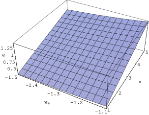
Figure 5: The ratio $g$ of total lifetimes versus the parameters $\xi=x$ and $\omega_{e}$ in the case of $\Omega_{e,0}=0.72$.

Next we turn to the coincidence problem. Following [21], we calculate the ratio of the period when the universe is in the coincidence state to the total lifetime of the universe. That is, we will calculate the quantity

$$f=\frac{t_{c}}{t_{U}},$$ (3.11)

where $t_{c}$ is defined by

$$t_{c}=H^{-1}_{0}\int^{a_{2}}_{a_{1}}da\ a^{1/2}[1-\Omega_{e,0}(1-a^{\xi})]^{3\omega_{e}/2\xi}.$$ (3.12)

During the coincidence state, the energy density of dark energy is comparable to that of dark matter and the scale factor evolves from $a_{1}$ to $a_{2}$. What is the exact meaning by the term “comparable”? This is not a well-defined question in order to determine the scale factors $a_{1}$ and $a_{2}$. In [21], Scherrer defined a scale of the energy density ratio $r_{0}$ so that the dark energy and dark matter densities are regarded as to be comparable if they differ by less than the ratio $r_{0}$ in either direction. He found that the ratio varies from $1/3$ to $1/8$ as $\omega_{e}$ varies from $-1.5$ to $-1.1$ if $r_{0}=10$ in a phantom dark energy model without interaction between the dark energy and dark matter. In this sense indeed the coincidence problem is significantly ameliorated in the phantom model because the ratio is not so small. As a result it is not so strange that we live in the epoch when the energy densities of dark energy and dark matter are of the same order. Now we want to see how the fraction varies when the phenomenological interaction is introduced.

The fraction of the total lifetime of the universe for which the universe is in the coincidence state, turns out to be

$$f = \frac{\int^{r_{0}}_{1/r_{0}}r^{3/2\xi-1}(1+r)^{3\omega_{e}/2\xi}dr}{\int^{\infty}_{0}r^{3/2\xi-1}(1+r)^{3\omega_{e}/2\xi}dr}$$ (3.13)

$$= \frac{\frac{2}{3}(r_{0}^{3/2\xi}\ {}_{2}F_{1}[\frac{3}{2\xi},-\frac{3\omega_{e}}{2\xi},1+\frac{3}{2\xi},-r_{0}]-r_{0}^{-3/2\xi}\ {}_{2}F_{1}[\frac{3}{2\xi},-\frac{3\omega_{e}}{2\xi},1+\frac{3}{2\xi},-\frac{1}{r_{0}}])}{\frac{\Gamma[3/2\xi]\Gamma[-3(1+\omega_{e})/2\xi]}{\Gamma[-3\omega_{e}/2\xi]}}.$$

Note that this ratio is independent of the current density parameter $\Omega_{e,0}$. In Fig. 6 and 7 we plot the ratio $f$ versus the scale $r_{0}$ for different parameters $\omega_{e}$ and $\xi$. Clearly for the case with fixed $\omega_{e}$ and $\xi$, a larger $r_{0}$ leads to a larger ratio $f$. On the other hand, for the case with fixed $r_{0}$ and $\omega_{e}$, a smaller $\xi$ gives us a larger ratio. For example, we see from Fig. 6 that when $r_{0}=10$ and $\omega_{e}=-1.5$, the ratio $f\sim 0.45$ for $\xi=3$, more large than the case ($f=1/3$) without the interaction. Note that the middle curve in Fig. 6 corresponds to the case without the interaction ($\xi=-3\omega_{e}$). In Fig. 8, we plot the ratio $f$ versus the parameters $\xi$ and $r_{0}$ for a fixed $\omega_{e}=-1.3$. From Fig. 6-8, one can see that indeed the period when the universe is in the coincidence state is comparable to its total lifetime. In addition, We note from (2.7) that a larger $\xi$ means that the universe will be dominated more quickly by the phantom dark energy, it corresponds to have a longer total lifetime of the universe, which can be seen from Fig. 4 and 5. Thus it is natural to have a smaller fraction $f$ than the case with a smaller $\xi$.

Figure 6: The ratio $f$ versus the parameter $r_{0}$ for the case of $\omega_{e}=-1.5$. Three curves from top to bottom correspond to the cases of $\xi=3$, $4.5$ and $5.5$, respectively.

Figure 7: The ratio $f$ versus the parameter $r_{0}$ for the case of $\omega_{e}=-1.1$. Three curves from top to bottom correspond to the cases of $\xi=2$, $3.3$ and $4$, respectively.

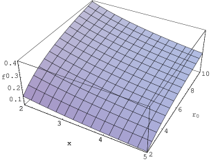
Figure 8: The ratio $f$ versus the parameters $r_{0}$ and $\xi$ for the case of $\omega_{e}=-1.3$. In the figure $x=\xi$.

4 Cosmology with a constant coupling parameter

In this section we consider the case with a constant coupling function $\delta$. In this case, we have the energy density of dark matter

$$\rho_{m}=\rho_{m,0}a^{-3+\delta}.$$ (4.1)

And then the dark energy density has the relation to the scale factor

$$\rho_{e}=\rho_{e,0}a^{-3+\delta+\xi}.$$ (4.2)

The Friedmann equation turns out to be

$$H^{2}=H^{2}_{0}(\Omega_{m,0}a^{-3+\delta}+\Omega_{e,0}a^{-3+\delta+\xi}).$$ (4.3)

In this case, the equation-of-state $\omega_{e}$ of the dark energy will depend on time (scale factor). From (2.2), we can obtain

$$\omega_{e}=-\frac{\delta+\xi}{3}-\frac{\delta}{3}\frac{\Omega_{m,0}}{\Omega_{e,0}}a^{-\xi}.$$ (4.4)

When $\delta=0$, one has $\xi=-3\omega_{e}$. This situation is just the case without the interaction. From (4.2) and (4.4), one can see that in order the dark energy to be phantom, $\delta+\xi>3$ has to be satisfied so that the dark energy density increases with the scale factor. When $\delta+\xi=3$, although the dark energy density keeps as a constant, it does not act as a cosmological constant due to the interaction between the dark energy and dark matter. We see from (4.4) that

$$\omega_{e}(a\to 0)=-sign(\delta)\cdot\infty,\ \ \omega_{e}(a\to 1)=-\frac{\delta+\xi}{3}-\frac{\delta}{3}\frac{\Omega_{m,0}}{\Omega_{e,0}},\ \ \ \omega_{e}(a\to\infty)=-\frac{\delta+\xi}{3}.$$ (4.5)

It is interesting to note that $\omega_{e}$ diverges as $a\to 0$. This is due to the fact that the dark energy density (4.2) approaches to zero very quickly, while the energy density of dark matter (4.1) goes to infinity as $a\to 0$, in order for the equation (2.2) to hold, the parameter $\omega_{e}$ has to go to infinity. In fact, the dark energy does not play any role at early times, which can be seen from the Friedmann equation (4.3). Therefore here the divergence of $\omega_{e}$ does not make any sense in physics.

The deceleration parameter is found to be

$$q=-1+\frac{1}{2}\frac{(3-\delta)\Omega_{m,0}+(3-\delta-\xi)\Omega_{e,0}a^{\xi}}{\Omega_{m,0}+\Omega_{e,0}a^{\xi}},$$ (4.6)

which has $q=-1+(3-\delta-\xi\Omega_{e,0})/2$ when $a=1$ and $q=(1-\delta-\xi)/2$ when $a\to\infty$. In Fig. 9 and 10 we plot the deceleration parameter versus the red shift for the case with a fixed $\xi=4$, different $\delta$, and the case with a fixed $\delta=0.3$, different $\xi$, respectively. Note that the coupling parameter $\delta$ will affect the expansion law (4.1) of dark matter density. We do not expect that the usual behavior ($\rho_{m}\sim a^{-3}$) will be changed much. So we take the value of $\delta$ so that the exponent is changed within $10\%$. That is, $\delta$ is taken to be in the range of $(-0.3,0.3)$. Of course, in order to get a correct constraint on the parameter $\delta$ from the observation data, a detailed numerical analysis has to be done. We see from Fig. 9 that for the case with a given $\xi$, a larger $\delta$ leads to a smaller red shift when the universe transits from a deceleration phase to an acceleration phase, while Fig. 10 tells us that for the case with a fixed $\delta$, a larger $\xi$ gives us a smaller red shift.

Figure 9: The deceleration parameter $q$ versus the red shift $z$ for the case of $\Omega_{e,0}=0.72$ and $\xi=4$. Three curves from top to bottom correspond to the cases $\delta=0.3$, $0$ and $-0.3$, respectively.

Figure 10: The deceleration parameter $q$ versus the red shift $z$ for the case of $\Omega_{e,0}=0.72$ and $\delta=0.3$. Three curves from bottom to top at the $q$ axis correspond to the cases $\xi=5$, $4$ and $3$, respectively.

From (4.3) we can get the total lifetime of the universe

$$t_{U}=H_{0}^{-1}\int^{\infty}_{0}da\ a^{-1}(\Omega_{m,0}a^{-3+\delta}+\Omega_{e,0}a^{-3+\delta+\xi})^{-1/2}.$$ (4.7)

We now consider the effect of the interaction on the total lifetime. Note that the total lifetime of the universe without the interaction is

$$t_{T}=H_{0}^{-1}\int^{\infty}_{0}da\ a^{-1}(\Omega_{m,0}a^{-3}+\Omega_{e,0}a^{-3+\xi})^{-1/2}.$$ (4.8)

Denote the ratio $t_{U}/t_{T}$ by $g$, we can express this as

$$g=\frac{\int^{\infty}_{0}dr(\frac{1-\Omega_{e,0}}{\Omega_{e,0}})^{(3-\delta)/2\xi}r^{(3-\delta-2\xi)/2\xi}(1+r)^{-1/2}}{\int^{\infty}_{0}dr(\frac{1-\Omega_{e,0}}{\Omega_{e,0}})^{3/2\xi}r^{(3-2\xi)/2\xi}(1+r)^{-1/2}}.$$ (4.9)

In Fig. 11, the ratio $g$ is plotted versus the parameters $\xi$ and $\delta$ for the case $\Omega_{e,0}=0.72$. We see that the case $\delta>0$ is quite different from the case of $\delta<0$. For the case with a fixed $\delta>0$, a larger $\xi$ leads to a longer lifetime of the universe. On the contrary, for the case with a fixed $\delta<0$, a smaller $\xi$ gives us a longer lifetime. Further, for the case with a fixed $\xi$, a smaller $\delta$ has a longer lifetime of the universe.

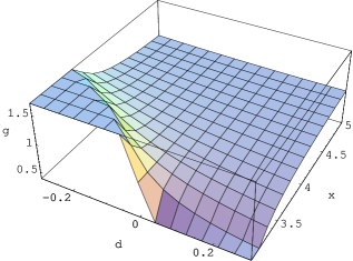
Figure 11: The ratio $g$ of total lifetimes versus the parameters $\xi=x$ and $\delta=d$ for the case of $\Omega_{e,0}=0.72$.

Finally we consider the fraction of the total lifetime for which the universe is in the coincidence state. As the case with a constant $\omega_{e}$ considered in the previous section, we calculate the following ratio:

$$f=\frac{\int^{r_{0}}_{1/r_{0}}dr\ r^{(3-\delta-2\xi)/2\xi}(1+r)^{-1/2}}{\int^{\infty}_{0}dr\ r^{(3-\delta-2\xi)/2\xi}(1+r)^{-1/2}}.$$ (4.10)

Figure 12: The ratio $f$ versus the parameter $r_{0}$ for a fixed $\xi=4$. Three curves from top to bottom correspond to the cases of $\delta=0.3$, $0$ and $-0.3$, and corresponding equation-of-state are $\omega_{e,0}=-1.47$, $-1.33$ and $-1.19$, respectively.

In Fig. 12 we plot the ratio $f$ versus the scale $r_{0}$ for a fixed $\xi$, but different $\delta$. It shows that a larger $\delta$ gives a larger ratio for a fixed $r_{0}$. On the other hand, we plot the ratio $f$ in Fig. 13 versus the scale $r_{0}$ for a fixed $\delta$, but different $\xi$, which shows that a larger $\xi$ gives us a larger ratio for a fixed $r_{0}$. Note that the case with $\omega_{e,0}=-1.80$ is already ruled out [11]. Here we draw this case just for illustration. Fig. 14 shows the relation of the ratio $f$ versus the parameters $\xi$ and $\delta$ for a fixed scale $r_{0}=5$.

Figure 13: The ratio $f$ versus the parameter $r_{0}$ for a fixed $\delta=0.3$. Three curves from top to bottom correspond to the cases of $\xi=5$, $4$ and $3$, and corresponding equation-of-state are $\omega_{e,0}=-1.80$, $-1.47$ and $-1.13$, respectively.

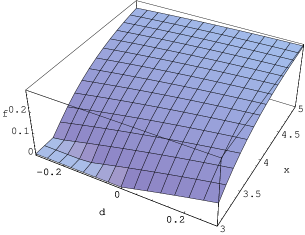
Figure 14: The ratio $f$ versus the parameters $\delta=d$ and $\xi=x$ for a given $r_{0}=5$.

5 Conclusion

In summary we discuss a cosmological model in which phantom dark energy has an interaction with dark matter. The interaction is introduced phenomenologically by considered an additional term [see (2.1) and (2.2)] in the equations of motion of dark energy and dark matter. This term is parameterized by a product of a dimensionless coupling function $\delta$, Hubble parameter and the energy density of dark matter, and it describes an energy flow between the dark energy and dark matter. We discuss two cases, one is the case where the equation-of-state $\omega_{e}=p_{e}/\rho_{e}$ of the dark energy is kept as a constant; the other corresponds to the case with a constant coupling function $\delta$. We investigate the effect of the interaction on the evolution of the universe, the total lifetime of the universe, and the fraction of the total lifetime of the universe for which the universe is in the coincidence state, where the energy densities of the dark energy and dark matter are comparable. We find that the interaction has rich and significant consequences on these issues. For example, the fraction of the total lifetime of the universe for which the universe is in the coincidence state can approximately reach $0.45$ if we take $\omega_{e}=-1.5$, $r_{0}=10$ and $\xi=3$. It means that the period when the energy densities of the dark energy and dark matter are comparable is significantly long, compared to its total lifetime. Thus, it is not so strange that we now live in the coincidence state of the universe. In this sense the coincidence problem can indeed be significantly ameliorated in such an interacting phantom dark energy model. Finally let us stress that the constraints on the parameters of the coupled dark energy model from the supernova Ia data has been analyzed recently [19] (see also [17, 18]), the values of parameters we take in this paper are all in the allowed region. Certainly it is not enough to consider the constraints from the supernova data only. We expect that the data from the cosmic microwave background radiation and in particular, from the large scale structure will give more restrictive constraints on this coupled dark energy model. This issue is currently under investigation.

Note added. After the manuscript was put on the net, we have been informed that a similar idea has also been considered by Z.K. Guo and Y.Z. Zhang. In addition, we have noticed that following [21], the coincidence problem has been discussed in a scalar field dark energy model with a linear effective potential [22].

References

- [1] A. G. Riess et al. [Supernova Search Team Collaboration], Astron. J. 116, 1009 (1998) [arXiv:astro-ph/9805201]; S. Perlmutter et al. [Supernova Cosmology Project Collaboration], Astrophys. J. 517, 565 (1999) [arXiv:astro-ph/9812133]; A. G. Riess et al. [Supernova Search Team Collaboration], Astrophys. J. 607, 665 (2004) [arXiv:astro-ph/0402512].
- [2] C. L. Bennett et al., Astrophys. J. Suppl. 148, 1 (2003) [arXiv:astro-ph/0302207]; D. N. Spergel et al. [WMAP Collaboration], Astrophys. J. Suppl. 148, 175 (2003) [arXiv:astro-ph/0302209].
- [3] M. Tegmark et al. [SDSS Collaboration], Phys. Rev. D 69, 103501 (2004) [arXiv:astro-ph/0310723]; K. Abazajian et al., arXiv:astro-ph/0410239; K. Abazajian et al. [SDSS Collaboration], Astron. J. 128, 502 (2004) [arXiv:astro-ph/0403325]. K. Abazajian et al. [SDSS Collaboration], Astron. J. 126, 2081 (2003) [arXiv:astro-ph/0305492]; E. Hawkins et al., Mon. Not. Roy. Astron. Soc. 346, 78 (2003) [arXiv:astro-ph/0212375]; L. Verde et al., Mon. Not. Roy. Astron. Soc. 335, 432 (2002) [arXiv:astro-ph/0112161].
- [4] S. Weinberg, Rev. Mod. Phys. 61, 1 (1989); P. J. E. Peebles and B. Ratra, Rev. Mod. Phys. 75, 559 (2003) [arXiv:astro-ph/0207347]; T. Padmanabhan, Phys. Rept. 380, 235 (2003) [arXiv:hep-th/0212290].
- [5] C. Wetterich, Nucl. Phys. B 302, 668 (1988); P. J. E. Peebles and B. Ratra, Astrophys. J. 325, L17 (1988); B. Ratra and P. J. E. Peebles, Phys. Rev. D 37, 3406 (1988); J. A. Frieman, C. T. Hill, A. Stebbins and I. Waga, Phys. Rev. Lett. 75, 2077 (1995) [arXiv:astro-ph/9505060]; M. S. Turner and M. J. White, Phys. Rev. D 56, 4439 (1997) [arXiv:astro-ph/9701138]; R. R. Caldwell, R. Dave and P. J. Steinhardt, Phys. Rev. Lett. 80, 1582 (1998) [arXiv:astro-ph/9708069]; A. R. Liddle and R. J. Scherrer, Phys. Rev. D 59, 023509 (1999) [arXiv:astro-ph/9809272]; P. J. Steinhardt, L. M. Wang and I. Zlatev, Phys. Rev. D 59, 123504 (1999) [arXiv:astro-ph/9812313]; D. F. Torres, Phys. Rev. D 66, 043522 (2002) [arXiv:astro-ph/0204504].
- [6] C. Armendariz-Picon, T. Damour and V. Mukhanov, Phys. Lett. B 458, 209 (1999) [arXiv:hep-th/9904075]; J. Garriga and V. F. Mukhanov, Phys. Lett. B 458, 219 (1999) [arXiv:hep-th/9904176].
- [7] T. Chiba, T. Okabe and M. Yamaguchi, Phys. Rev. D 62, 023511 (2000) [arXiv:astro-ph/9912463]; C. Armendariz-Picon, V. Mukhanov and P. J. Steinhardt, Phys. Rev. Lett. 85, 4438 (2000) [arXiv:astro-ph/0004134]. C. Armendariz-Picon, V. Mukhanov and P. J. Steinhardt, Phys. Rev. D 63, 103510 (2001) [arXiv:astro-ph/0006373]; T. Chiba, Phys. Rev. D 66, 063514 (2002) [arXiv:astro-ph/0206298].
- [8] A. Vikman, arXiv:astro-ph/0407107.
- [9] R. M. Wald, General Relativity, Chicago University Press, 1984.
- [10] R. R. Caldwell, Phys. Lett. B 545, 23 (2002) [arXiv:astro-ph/9908168].
- [11] R. A. Knop et al., Astrophys. J. 598, 102 (2003) [arXiv:astro-ph/0309368]; A. G. Riess et al. [Supernova Search Team Collaboration], Astrophys. J. 607, 665 (2004) [arXiv:astro-ph/0402512].
- [12] P. F. Gonzalez-Diaz, Phys. Rev. D 68, 021303 (2003) [arXiv:astro-ph/0305559]; S. Nojiri and S. D. Odintsov, Phys. Lett. B 595, 1 (2004) [arXiv:hep-th/0405078]; S. Nojiri and S. D. Odintsov, arXiv:hep-th/0408170; E. Elizalde, S. Nojiri and S. D. Odintsov, Phys. Rev. D 70, 043539 (2004) [arXiv:hep-th/0405034]; P. X. Wu and H. W. Yu, arXiv:astro-ph/0407424; Z. K. Guo, Y. S. Piao, X. M. Zhang and Y. Z. Zhang, arXiv:astro-ph/0410654; B. Feng, M. Li, Y. S. Piao and X. Zhang, arXiv:astro-ph/0407432.
- [13] V. K. Onemli and R. P. Woodard, Class. Quant. Grav. 19, 4607 (2002) [arXiv:gr-qc/0204065]; V. K. Onemli and R. P. Woodard, arXiv:gr-qc/0406098; T. Brunier, V. K. Onemli and R. P. Woodard, arXiv:gr-qc/0408080; B. Boisseau, G. Esposito-Farese, D. Polarski and A. A. Starobinsky, Phys. Rev. Lett. 85, 2236 (2000) [arXiv:gr-qc/0001066].
- [14] R. R. Caldwell, M. Kamionkowski and N. N. Weinberg, Phys. Rev. Lett. 91, 071301 (2003) [arXiv:astro-ph/0302506]; S. Nesseris and L. Perivolaropoulos, arXiv:astro-ph/0410309.
- [15] L. Amendola, Phys. Rev. D 62, 043511 (2000) [arXiv:astro-ph/9908023]; X. l. Chen and M. Kamionkowski, Phys. Rev. D 60, 104036 (1999) [arXiv:astro-ph/9905368]; J. P. Uzan, Phys. Rev. D 59, 123510 (1999) [arXiv:gr-qc/9903004]; F. Perrotta, C. Baccigalupi and S. Matarrese, Phys. Rev. D 61, 023507 (2000) [arXiv:astro-ph/9906066]. T. Chiba, Phys. Rev. D 60, 083508 (1999) [arXiv:gr-qc/9903094]; A. P. Billyard and A. A. Coley, Phys. Rev. D 61, 083503 (2000) [arXiv:astro-ph/9908224]; V. Faraoni, Phys. Rev. D 62, 023504 (2000) [arXiv:gr-qc/0002091]; L. P. Chimento, A. S. Jakubi and D. Pavon, Phys. Rev. D 62, 063508 (2000) [arXiv:astro-ph/0005070]; A. B. Batista, J. C. Fabris and R. de Sa Ribeiro, Gen. Rel. Grav. 33, 1237 (2001) [arXiv:gr-qc/0001055]; R. Bean and J. Magueijo, Phys. Lett. B 517, 177 (2001) [arXiv:astro-ph/0007199]; A. A. Sen and S. Sen, Mod. Phys. Lett. A 16, 1303 (2001) [arXiv:gr-qc/0103098]; W. Zimdahl and D. Pavon, Phys. Lett. B 521, 133 (2001) [arXiv:astro-ph/0105479]; T. Chiba, Phys. Rev. D 64, 103503 (2001) [arXiv:astro-ph/0106550]; G. Esposito-Farese and D. Polarski, Phys. Rev. D 63, 063504 (2001) [arXiv:gr-qc/0009034].
- [16] A. Bonanno and M. Reuter, Phys. Lett. B 527, 9 (2002) [arXiv:astro-ph/0106468]; A. Gromov, Y. Baryshev and P. Teerikorpi, arXiv:astro-ph/0209458; M. B. Hoffman, arXiv:astro-ph/0307350; U. Franca and R. Rosenfeld, Phys. Rev. D 69, 063517 (2004) [arXiv:astro-ph/0308149]; M. Axenides and K. Dimopoulos, JCAP 0407, 010 (2004) [arXiv:hep-ph/0401238]; T. Biswas and A. Mazumdar, arXiv:hep-th/0408026; F. Piazza and S. Tsujikawa, JCAP 0407, 004 (2004) [arXiv:hep-th/0405054]; W. Zimdahl and D. Pavon, Gen. Rel. Grav. 35, 413 (2003) [arXiv:astro-ph/0210484]; W. Zimdahl and D. Pavon, Gen. Rel. Grav. 36, 1483 (2004) [arXiv:gr-qc/0311067]; D. Pavon, S. Sen and W. Zimdahl, JCAP 0405, 009 (2004) [arXiv:astro-ph/0402067].
- [17] N. Dalal, K. Abazajian, E. Jenkins and A. V. Manohar, Phys. Rev. Lett. 87, 141302 (2001) [arXiv:astro-ph/0105317].
- [18] L. Amendola, M. Gasperini and F. Piazza, arXiv:astro-ph/0407573.
- [19] E. Majerotto, D. Sapone and L. Amendola, arXiv:astro-ph/0410543.
- [20] B. McInnes, arXiv:astro-ph/0210321.
- [21] R. J. Scherrer, arXiv:astro-ph/0410508.
- [22] P. P. Avelino, arXiv:astro-ph/0411033.