Abstract

We study the behaviour of spinning strings in the background of various distributions of smeared giant gravitons in supergravity. This gives insights into the behaviour of operators of high dimension, spin and R–charge. Using a new coordinate system recently presented in the literature, we find that it is particularly natural to prepare backgrounds in which the probe operators develop a variety of interesting new behaviours. Among these are the possession of orbital angular momentum as well as spin, the breakdown of logarithmic scaling of dimension with spin in the high spin regime, and novel splitting/fractionation processes.

1 Introduction

1.1 Background

Recently, in ref.[1] a new coordinate system was discovered which allows for a rather general description of the type IIB supergravity duals of 1/2–BPS states in ${\cal N}=4$ supersymmetric Yang–Mills theory. Specifically, metric is:

$$ds^{2} = -h^{-2}(dt+V_{i}dx^{i})^{2}+h^{2}(dy^{2}+dx^{i}dx^{i})+ye^{G}d\Omega_{3}^{2}+ye^{-G}d{\tilde{\Omega}}_{3}^{2}\ ,$$

$$h^{-2} = 2y\cosh G\ ,\quad y\partial_{y}V_{i}=\epsilon_{ij}\partial_{j}z\ ,$$ (1)

$$\hskip-56.9055pt\quad y(\partial_{i}V_{j}-\partial_{j}V_{i})=\epsilon_{ij}\partial_{y}z\ ,\quad z=\frac{1}{2}\tanh G\ ,$$

where $i,j=1,2$ , and $z$ obeys the equation

$$\partial_{i}\partial_{j}z+y\partial_{y}\left(\frac{\partial_{y}z}{y}\right)=0\ .$$ (2)

There is no axion or dilaton field, nor are the three–form potentials non–zero. The five–form field strength is non–zero, but we will not list it here.

Notably, the $(x^{1},x^{2})$ plane defined by setting the coordinate $y$ to zero is isomorphic to the phase space of the fermionic description of 1/2–BPS states introduced in ref.[2]. On this plane, the function $z$ must take one of the values $\pm\frac{1}{2}$ in order for the metric to be non–singular. Imagine colouring the plane black where $z=-\frac{1}{2}$ and white where $z=+\frac{1}{2}$. Then one has a patchwork of shapes on the plane giving the boundary condition for the function $z$. The differential equation (2) supplies a solution for $z$ everywhere and this gives the entire ten dimensional metric.

The plane is to be thought of as a realization of the fermionic phase space of the matrix model description of the 1/2–BPS states as given in ref.[2]. The simplest configuration is a circular disc centered at the origin. This Fermi droplet, filled out to radius $r_{0}$ (determined by the fact that there are $N$ fermions in the droplet and that there is a minimum area allowed a single fermion), is in fact simply AdS${}_{5}\times S^{5}$ with radius $R^{2}=r_{0}$, which is set by the $N$ of the ${\cal N}=4$ supersymmetric $SU(N)$ gauge theory to which it is dual in the usual way:

$$R^{4}=4\pi(\alpha^{\prime})^{2}g_{s}N=2(\alpha^{\prime})^{2}\lambda\ ;\qquad\lambda=g^{2}_{\rm YM}N\ .$$ (3)

Defining cylindrical polars $(r,\phi)$ in the $(x_{1},x_{2})$ plane, the coordinates relate to the familiar global AdS${}_{5}\times S^{5}$ coordinates in the following way:

$$y=r_{0}\sinh\!\rho\sin\theta\ ,\qquad r=r_{0}\cosh\!\rho\cos\theta\ ,\quad\phi={\tilde{\phi}}+t\ ,$$ (4)

where the metric is:

$$ds^{2}=r_{0}\left(d\rho^{2}-\cosh^{2}\rho dt^{2}+\sinh^{2}\rho d\Omega_{3}^{2}+d\theta^{2}+\cos^{2}\theta d{\tilde{\phi}}^{2}+\sin^{2}\theta d{\tilde{\Omega}}_{3}^{2}\right)\ .$$ (5)

Inside the disc,(see figure 1), $z=-\frac{1}{2}$, and $\rho=0$, so $r$ runs from $0$ to $r_{0}$ as $\theta$ runs from $\frac{\pi}{2}$ to $0$. The $S^{3}$ of AdS₅ is collapsed in the interior, while that of the $S^{5}$, denoted ${\tilde{S}}^{3}$, has radius set by $\sqrt{r_{0}}\sin\theta$. So it shrinks to zero on the boundary of the disc. So $\theta=0$ is the pole of the $S^{5}$. Beyond the disc, $\theta=0$ and $\rho$ runs from $0$ to $\infty$. The $S^{3}$ has radius $\sqrt{r_{0}}\sinh\rho$, and we construct AdS₅.

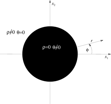
Figure 1: The configuration which corresponds to AdS${}_{5}\times S^{5}$.

A small hole inside the disc corresponds to a giant graviton[3], i.e., some D3–branes wrapped on an $S^{3}$ within the $S^{5}$. See figure 2(a). It is a spinning configuration, moving with constant angular speed on the polar coordinate $\phi$ of the $S^{5}$. Notice that how much the hole is radially displaced in the plane sets where in $\theta$ the giant graviton is located, and the size of the ${\tilde{S}}^{3}$ changes with radius. Radius translates into angular momentum. Notice that the limit to the size of the giant graviton (since it must fit inside the $S^{5}$)[3]) is very easy to visualize in this picture: The hole can only live inside the disc.

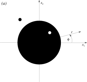
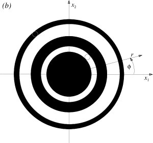
Figure 2: (a): The configurations which correspond to giant gravitons on the $S^{5}$ (the hole), and giant gravitons on the AdS₅ (the particle). They all have angular momentum in the $\tilde{\phi}$ direction on the $S^{5}$. (b): Smearing the giant (and dual giant) gravitons of part (a).

Placing a small droplet at some place outside of the disc (see figure 2(a)) corresponds to a dual giant graviton[4, 5], i.e., some D3–branes wrapping an $S^{3}$ of AdS₅. At the edge of the disc, it has zero size (since the $S^{3}$ is of zero radius there) but then it can be moved to arbitrary $\rho$: It can be given arbitrary angular momentum in the $S^{5}$.

That the droplets represent spinning objects moving in ${\tilde{\phi}}$ is clear from the change of variables given in equation (4), since they are at fixed ${\phi}$. Any solution which is symmetric in $\phi$ will be time–independent. The disc discussed above is the simplest example. For another example, we can construct a solution representing a distribution of dual (AdS₅) giants by smearing a droplet into a ring. For a thin ring, this is a good description. Amusingly, for an increasingly thicker ring, it is increasingly valid to think of this configuration as representing smeared $S^{5}$ giants in the context of a new AdS${}_{5}\times S^{5}$ geometry whose scale is set by the size of the outer radius of the ring. Clearly, similar statements can be made about the case of smearing giants into a thick ring. See figure 2(b)).

1.2 Motivation

These coordinates are extremely powerful for describing 1/2–BPS states and deserve to be explored and better understood. This is one of the goals of this project. Generally, there are very simple questions in the dual gauge theory which at times have seemed rather hard to capture in supergravity. Many pieces of work, often guided by natural probes of the geometry and the gauge theory (see e.g., refs.[6, 7, 8, 9]) have shown that this often boils down to a matter of finding good coordinates on the gravity side. Recent work has shown that many seemingly complicated gravity duals of e.g. various holographic RG flows[10, 11, 12], and now these 1/2–BPS state geometries[1], are in fact very simple, if expressed in the right coordinates. The solutions are seeded by a simple function, with non–trivial dependence on a submanifold of the ten–dimensional geometry, satisfying a differential equation (here it is equation (2)). On the basis of probe computations, it has been suggested[13] that these sorts of coordinates are probably pointing to an underlying reduced model (perhaps a matrix model or integrable system) and this is precisely what the coordinates of ref.[1] have shown, for the case of 1/2–BPS states, by making the gauged harmonic oscillator model of ref.[2] extraordinarily manifest in the geometry.

Whether such a direct uncovering within the supergravity geometry of such a key ingredient of the reduced model (such as a phase space of the fermion basis of the matrix model) can be achieved for geometries which preserve fewer supersymmetries is an issue deserving further investigation. This is one the main motivations for studying the geometry of ref.[1] further in this paper.

It is families of concentric rings which we will consider in this paper, using them as a background in which we place spinning strings. These strings are known[14] to be dual to certain near BPS operators in the gauge theory, about which much has been learned in recent times. We will find in this paper that the backgrounds we prepare allow these strings (and hence operators in the dual theory) to take on new types of behaviour. For example, in addition to spin and R–charge, they can have orbital angular momentum as well. Further, their characteristic dependence for large and small spin (established in ref.[14]) is joined by an intermediate regime where they behave differently. There, depending upon the details of the background, they can split and join, redistributing the angular momentum and R–charge in various ways. They also have a high energy/spin regime which has a different scaling behaviour than that known for the long string regime, which exhibits logarithmic scaling with spin for the anomalous dimension of the associated operator[14]. In the next few sections, we show how to uncover these new pieces of physics.

2 Smeared Giants and Concentric Rings

First, let us show how to describe families of concentric rings. This is a review of material already presented in ref.[1]. The metric with polar coordinates in the $(x^{1},x^{2})$ plane is:

$$ds^{2}=-h^{-2}(dt+V_{r}dr+V_{\phi}d\phi)^{2}+h^{2}(dy^{2}+dr^{2}+r^{2}d\phi^{2})+ye^{G}d\Omega_{3}^{2}+ye^{-G}d\widetilde{\Omega}_{3}^{2}\ ,$$ (6)

If we define $\widetilde{z}=z-\frac{1}{2}$, it can be shown[1] that the solutions for $\widetilde{z}$, $V_{r}$ and $V_{\phi}$ are:

$$\widetilde{z} = \sum_{i}(-1)^{i+1}\left(\frac{r^{2}-(r^{(i)}_{0})^{2}+y^{2}}{2\sqrt{(r^{2}+(r^{(i)}_{0})^{2}+y^{2})^{2}-4r^{2}(r^{(i)}_{0})^{2}}}-\frac{1}{2}\right),$$

$$V_{r} = 0,$$

$$V_{\phi} = \frac{1}{2}\sum_{i}(-1)^{i}\left(\frac{r^{2}+y^{2}+(r^{(i)}_{0})^{2}}{\sqrt{(r^{2}+(r^{(i)}_{0})^{2}+y^{2})^{2}-4r^{2}(r^{(i)}_{0})^{2}}}-1\right)$$ (7)

Here $r^{(1)}_{0}$ is the radius of the outermost circle, $r^{(2)}_{0}$ the next one and so on. In the case of one radius, $r_{0}$, this is just the case of AdS${}_{5}\times S^{5}$.

3 Spinning Strings

Our next step is to study configurations of spinning strings in the geometry. The configurations which we study always the strings at have $r=0$. This symmetric situation will allow for a dramatic simplification of the equations governing the configurations. Having $r=0$ will mean that we keep the string at $\theta=\pi/2$ so that we can have non–trivial $\rho$ dependence.

If we parameterize the $S^{3}$ and $\widetilde{S}^{3}$ with the standard Euler angles: ($\alpha,\beta,\gamma$), and ($\widetilde{\alpha},\widetilde{\beta}$, $\widetilde{\gamma}$) respectively, then it can be shown that the following ansatz is compatible with the equations of motion derived from the sigma model action:

$$t = \kappa\tau\ ;\quad\phi=0\ ;\quad\alpha=\widetilde{\alpha}=0\ ;$$

$$r = \dot{y}=0\ ;\quad\beta+\gamma=\omega\tau\ ;\quad\widetilde{\beta}+\widetilde{\gamma}=\widetilde{\omega}\tau\ .$$ (8)

We denote the world–sheet time and space coordinates by $\tau$ and $\sigma$ respectively.

For this ansatz the only non–trivial equation of motion is the one for $y(\sigma)$ and it has the form:

$$\frac{y^{\prime\prime}}{y\cosh{G}}+\partial_{y}\left(\frac{1}{2y\cosh{G}}\right)y^{\prime 2}=\partial_{y}(2y\cosh{G})\kappa^{2}-\partial_{y}(ye^{G})\omega^{2}-\partial_{y}(ye^{-G})\widetilde{\omega}^{2}\ .$$ (9)

However it is more convenient to work with the Virasoro constraint which in this case is the first integral of the equation of motion and can be written as:

$$\frac{y^{\prime 2}}{e^{G}+e^{-G}}+y^{2}\left(e^{G}\omega^{2}+e^{-G}\widetilde{\omega}^{2}-\kappa^{2}(e^{G}+e^{-G})\right)=0\ .$$ (10)

Now using the fact that

$$e^{G}=\sqrt{\frac{1+\widetilde{z}}{-\widetilde{z}}}\ ,$$ (11)

and after a bit of algebra we arrive at the equation:

$$y^{\prime 2}=y^{2}\left(\frac{a}{\widetilde{z}}+\frac{b}{1+\widetilde{z}},\right)\ ,$$ (12)

where:

$$\widetilde{z}=\sum_{i}(-1)^{i}\frac{{(r^{(i)}_{0})^{2}}}{{(r^{(i)}_{0})^{2}}+{y^{2}}}\ ,\quad\mbox{\rm and}\quad a=\omega^{2}-\kappa^{2}\ ,\quad b=\kappa^{2}-\widetilde{\omega}^{2}\ .$$ (13)

If we consider the case $a>0,b>0$ (and we can do so without loss of generality) then we can write:

$$y^{\prime 2}=\frac{y^{2}a}{1+{\widetilde{z}}}\left(1+\eta+\frac{1}{\widetilde{z}}\right)\ ,\qquad\eta=\frac{b}{a}\ .$$ (14)

Note that $-1<\widetilde{z}<0$.

Now the condition for having a closed (folded) string is equivalent to the condition for having a bound state of the effective one dimensional motion described by (14). Since the factor outside the brackets is always positive, and since $1/{\widetilde{z}}$ is negative, we have a natural effective potential problem where the “energy” is set by the parameter ${\cal E}=1+\eta$ and the effective potential is:

$$V(y)=-\frac{1}{\widetilde{z}}\ .$$ (15)

The well–known case[14] of a folded string in AdS${}_{5}\times S^{5}$ is obtained by setting all the $r_{0}^{(i)}$ to zero except for one, called $r_{0}$. The effective potential is then simply $1+y^{2}/r_{0}^{2}$. The physics is then straightforward. The folded string configuration corresponds to a solution $y(\sigma)$ representing a string of finite extent stretching between the extremes given by the turning points of our associated particle problem. See figure 3.

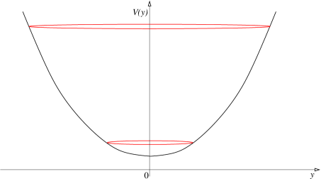
Figure 3: The effective potential for spinning string configurations in AdS${}_{5}\times S^{5}$. Shown is a short string and a long string.

The turning points are further apart (the folded string is longer) as the parameter $1+\eta$ is increased. In the limit where the string is short compared to the scale set by $r_{0}$ and the setting is effectively in flat space. The characteristic Regge behaviour, where the energy of the string scales as the square root of the spin, is recovered in this limit. There is an opposite limit where the strings are long compared to the scale set by $r_{0}$. There, the AdS physics is important, and the resulting string’s energy scales linearly with the spin, with logarithmic subleading behaviour[14]. We will recover all of this explicitly shortly.

The key point for us is that the new coordinates allow us to explore more complicated background configurations (or background operators in the dual gauge theory) quite simply. The new effective potentials obtained allow for multiple turning points as a function of ${\cal E}$. This will introduce many new allowed configurations, and new physics.

3.1 Sample Backgrounds

Two of our favourite configurations are as follows. Set $n$ to be the number of radii, which we choose to be odd, so as to have a black disc in the middle of the configuration and $n-1$ rings. The case of one radius will just be the original AdS${}_{5}\times S^{5}$. The configurations are:

$$\mbox{\rm Configuration 1}: r_{0}^{(i)}=i^{m}\ ,\qquad m\in{}^{+}\ .$$

$$\mbox{\rm Configuration 2}: r_{0}^{(i)}=q^{(i-1)}\ ,\qquad q\in\IR\ .$$ (16)

A four–ring example of Configuration 1 is drawn in figure 4. Samples of the effective potentials $V(y)$ resulting from these configurations, for a large number of rings, have been plotted in figures 5 and 6. (Beware the use of logarithmic scales on some axes.) Notice the existence of many minima, in addition to the overall minimum at $y=0$. These introduce new physics. Notice also that for large enough $y$ we recover the monotonic rise associated to the large $\rho$ (or $y$) behaviour of the overall AdS geometry.

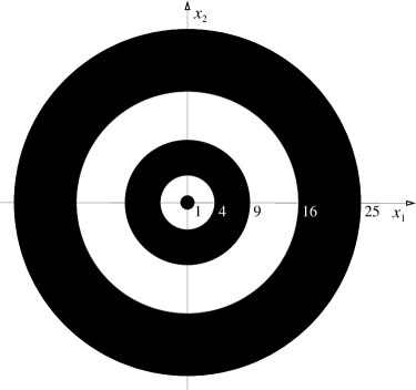
Figure 4: A set of rings, for Configuration 1, with $m=2$.

Among the new pieces of physics are the following: First, there are solutions (pairs of turning points) corresponding to folded strings with centres of mass which are located away from $y=0$. For these solutions the angular momentum splits into a spin, $S$, about the centre of mass, and an orbital angular momentum piece, $L$, since their motion on the $S^{3}$ is at finite $y$. This orbital angular momentum survives even in the point particle limit, in contrast to the case of the centred string. In the case of the latter, the point particle limit gives a BPS state in the limit, since $S$ and $L$ vanish. For the non–centred strings, their finite orbital angular momentum takes them off BPS. Note that for Configuration 1 (above), the potential is such that the deviation from BPS for the point particle configurations found in its extra minima is tunably small, since the minima are close to degenerate with the $y=0$ minimum. The “energy” in the potential is set by $\eta$, which can be tuned arbitrarily close to zero. Configuration 1 allows us to describe a family of minima which are almost degenerate with the global minimum. We will discuss this further later.

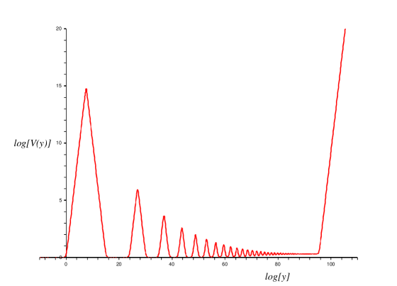
Figure 5: The effective potential $V(y)$ for the case of Configuration 1, with $m=50$, and $n=81$.

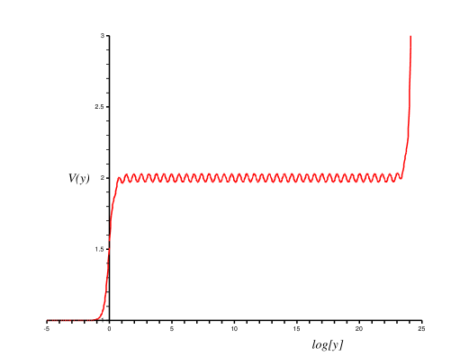
Figure 6: The effective potential $V(y)$ for the case of Configuration 2, with $q=2$, and $n=81$.

3.2 Short Strings and Regge Trajectories

Let us consider the case of a short string bound in the region between $y=0$ and the first zero of the term in the brackets in equation (14), located at $y=y_{0}$. Alternatively, we can think of this bound state as lying between $-y_{0}$ and $y_{0}$. See the lowest central string in figure 8. Our expressions for the energy, $E$ and the angular momentum $K$ of the string are:

$$E=\frac{\kappa}{2\pi\alpha^{\prime}}\int\limits^{2\pi}_{0}d\sigma{\left(2y\cosh{G}\right)}\ ,\qquad K=\frac{\omega}{2\pi\alpha^{\prime}}\int\limits^{2\pi}_{0}d\sigma{\left(ye^{G}\right)}\ .$$ (17)

Note that since we are considering an odd number of radii, this means that the conserved quantity associated with rotation in $S^{3}$ is the angular momentum of the particle (this is so because we are at center of the ring system $r=0$). Let us expand the left hand side of equation (14) to second order in $y$:

$$y^{\prime 2} = \frac{b}{f_{0}}-\left(a-b\frac{f_{1}}{f_{0}^{2}}\right)y^{2}+O(y^{4})\ ,$$

$$\frac{1}{f_{0}} = \sum_{i}(-1)^{i+1}\frac{1}{{r^{(i)}_{0}}^{2}}\ ,\quad\frac{1}{f_{1}}=\sum_{i}(-1)^{i+1}\frac{1}{{r^{(i)}_{0}}^{4}}\ .$$ (18)

Therefore the conditions for having a singly folded string with radius $y_{0}\ll 1$ are:

$$a-b\frac{f_{1}}{f_{0}^{2}}=1 y_{0}^{2}=\frac{b}{f_{0}}$$ (19)

Now if we consider rotation only in $S^{3}$, i.e., $\widetilde{\omega}=0$, then from the definitions of $a$ and $b$ in (13) it follows that:

$$y_{0}^{2}=\frac{\kappa^{2}}{f_{0}}\ ,\quad\omega^{2}=1+\kappa^{2}\left(1+\frac{f_{1}}{f_{0}^{2}}\right)\ ,\quad\kappa\ll 1\ .$$ (20)

Expanding the integrands in equation (17) to second order in $y$ leads to the expressions for the energy, $E$, and spin, $S$:

$$E=\frac{\kappa}{2\pi\alpha^{\prime}}\int\limits^{2\pi}_{0}d\sigma{\frac{1}{\sqrt{f_{0}}}}+O(\kappa^{3})=\frac{\kappa}{\alpha^{\prime}}\frac{1}{\sqrt{f_{0}}}+O(\kappa^{3})\ ,$$

$$S=\frac{\omega}{2\pi\alpha^{\prime}}\int\limits^{2\pi}_{0}d\sigma{\frac{\kappa^{2}}{\sqrt{f_{0}}}}\sin^{2}\sigma=\frac{\kappa^{2}}{4\pi\alpha^{\prime}\sqrt{f_{0}}}+O(\kappa^{4})\ .$$ (21)

From this we see that for short strings ($\kappa\ll 1$) we have the Regge trajectories:

$$E^{2}=\frac{4\pi\sqrt{f_{0}}}{\alpha^{\prime}}S\ .$$ (22)

The quantity $f_{0}$ given in equation (18), acts as an effective AdS radius in the problem in this limit. For the one radius (i.e., disc) problem the result of ref.[14] for AdS is reproduced. See figure 7 for a numerical plot of this behaviour for a three–ring example.

It is possible to tune the location of the ring radii to obtain other minima, as is evident from our examples in the previous subsection.

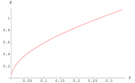
Figure 7: Plots of $E$ vs $S$ showing Regge behaviour for a spinning string in the short string regime.

3.3 Particles and Short Strings at $y\neq 0$

Consider the solutions corresponding to the extra minima that can be generated by our effective potential $V(y)=-1/{\widetilde{z}}$. Denote the position of the $i$th extra minimum by $y_{0}^{(i)}$.

Let us first study the point–like solutions corresponding to string positioned at the bottom of the potential well, collapsed to a particle. We can do that by tuning $\eta$ appropriately. Let’s denote its corresponding value by $\eta^{(i)}$. Then we have the relation for our point–like configurations:

$$1+\eta^{(i)}=-\frac{1}{\widetilde{z}(y_{0}^{(i)})}\ .$$ (23)

Let’s compute the conserved quantities related to $\omega,\widetilde{\omega}$ and $\kappa$. For point–like strings they are simply (using equation (11)):

$$E_{0}^{(i)}=\frac{\kappa^{(i)}}{\alpha^{\prime}}2\cosh{G}|_{y_{0}^{(i)}}=\frac{\kappa^{(i)}}{\alpha^{\prime}}y_{0}^{(i)}\left(\sqrt{\eta^{(i)}}+\frac{1}{\sqrt{\eta^{(i)}}}\right)$$ (24)

$$L_{0}^{(i)}=\frac{\omega^{(i)}}{\alpha^{\prime}}ye^{G}|_{y_{0}^{(i)}}=\frac{\omega^{(i)}}{\alpha^{\prime}}y_{0}^{(i)}\sqrt{\eta^{(i)}}$$ (25)

$$J_{0}^{(i)}=\frac{\widetilde{\omega}^{(i)}}{\alpha^{\prime}}ye^{-G}|_{y_{0}^{(i)}}=\frac{\widetilde{\omega}^{(i)}}{\alpha^{\prime}}y_{0}^{(i)}\frac{1}{\sqrt{\eta^{(i)}}}$$ (26)

Let us define, for convenience, a parameter $\zeta=(\frac{\omega}{\widetilde{\omega}})^{2}$. It can be verified that from $\eta\geq 0$ follows $\zeta\geq 1$. We can now check the BPS condition. After a bit of algebra we find:

$$\frac{E^{(i)}-J^{(i)}}{J^{(i)}}=\frac{\Delta^{(i)}-J^{(i)}}{J^{(i)}}=\sqrt{1+\eta^{(i)}}\sqrt{1+\zeta^{(i)}\eta^{(i)}}-1\geq 0\ .$$ (27)

Notice that since $\zeta$ is not bounded from above, we can go as far as we wish from the BPS condition. This is not surprising because now we are free to increase the (orbital) angular momentum, $L_{0}^{(i)}$, of the particle in the $S^{3}$ without changing the corresponding one in $\widetilde{S}^{3}$ which is the R–charge $J^{(i)}$. However if we fix $\zeta$ and tune $\eta^{(i)}$ close to zero, we can make the corresponding operator as close to BPS as wish. It is natural because from (24) we can see that $L_{0}\rightarrow 0$ as $\sqrt{\eta}\rightarrow 0$. So in the Configuration 1 example that we gave, since the minima are all degenerate with the $y=0$ minimum, this is the case.

We now study short strings corresponding to the harmonic approximation for the effective potential around the minima $y_{0}^{(i)}$. For this purpose we can expand:

$$y=y_{0}^{(i)}+\xi\ .$$ (28)

Now if we expand our effective potential we have:

$$-\frac{1}{\widetilde{z}(\xi)}=1+\eta^{(i)}+\frac{\widetilde{z}^{\prime\prime}(y_{0}^{(i)})}{2\widetilde{z}(y_{0}^{(i)})^{2}}\xi^{2}+O(\xi^{3})\ .$$ (29)

Therefore the equation of motion for $\xi$ is:

$$\xi^{\prime 2} = \left.\frac{ay^{2}\widetilde{z}^{\prime\prime}}{2(1+\widetilde{z})\widetilde{z}^{2}}\right|_{y_{0}^{(i)}}(\xi_{0}^{2}-\xi^{2})+O(\xi_{0}^{3})\ ,$$

$$\xi_{0}^{2} = (\eta-\eta_{0}^{(i)})\left.\frac{2\widetilde{z}^{2}}{\widetilde{z}^{\prime\prime}}\right|_{y_{0}^{(i)}}$$ (30)

Now the periodicity condition (for having singly folded string) implies:

$$a=a^{(i)}=\left.\frac{2(1+\widetilde{z})\widetilde{z}^{2}}{y^{2}\widetilde{z}^{\prime\prime}}\right|_{y_{0}^{(i)}}\ ,$$ (31)

and we have the solution:

$$y=y_{0}^{(i)}+\xi_{0}\sin\sigma\ .$$ (32)

The next step is to substitute (32) into the general expressions for the conserved quantities $E$, $K$ and $J$. Before proceeding, let us note that from here on, in order to simplify the notation we’ll omit the upper index $(i)$ denoting that everything that we write holds for the $i^{th}$ minimum. It should be clear from the context.

Only even powers of $\xi$ will contribute under the integral and so using:

$$e^{G} = \sqrt{\eta_{0}}(1+\Omega^{2}\xi_{0}^{2}\sin^{2}{\sigma})+O(\xi_{0}^{3})$$

$$e^{-G} = \frac{1}{\sqrt{\eta_{0}}}(1-\Omega^{2}\xi_{0}^{2}\sin^{2}{\sigma})+O(\xi_{0}^{3})\ ,$$ (33)

where we have introduced

$$\Omega^{2}=\left.\frac{\widetilde{z}^{\prime\prime}}{4\eta_{0}\widetilde{z}^{2}}\right|_{y_{0}}\ ,$$ (34)

we arrive at the energy, total angular momentum, and R–charge:

$$E=\frac{{\kappa}y_{0}}{\alpha^{\prime}}(\sqrt{\eta_{0}}+\frac{1}{\sqrt{\eta_{0}}})\left(1+\frac{1}{4\pi}\frac{\eta_{0}-1}{\eta_{0}+1}\Omega^{2}\xi_{0}^{2}\right)+O(\xi_{0}^{4})\ ,$$

$$K=\frac{{\omega}y_{0}}{\alpha^{\prime}}\sqrt{\eta_{0}}\left(1+\frac{1}{4\pi}\Omega^{2}\xi_{0}^{2}\right)+O(\xi_{0}^{4})\ ,$$

$$J=\frac{{\widetilde{\omega}}y_{0}}{\alpha^{\prime}}\frac{1}{\sqrt{\eta_{0}}}\left(1-\frac{1}{4\pi}\Omega^{2}\xi_{0}^{2}\right)+O(\xi_{0}^{4})\ .$$ (35)

Now let’s study the case when we don’t have R–charge, i.e., $\widetilde{\omega}=0$. Then from equation (31) and the definition for $\eta$ we get that:

$$\kappa^{2} = a^{(i)}\eta_{0}(1+2\Omega^{2}\xi_{0}^{2})\ ,$$

$$\omega^{2} = a^{(i)}(1+\eta)\left(1+2\frac{\eta_{0}}{1+\eta_{0}}\Omega^{2}\xi_{0}^{2}\right)\ .$$ (36)

Therefore:

$$E=y_{0}\frac{\sqrt{a^{(i)}\eta_{0}}}{\alpha^{\prime}}(\sqrt{\eta_{0}}+\frac{1}{\sqrt{\eta_{0}}})\left(1+\left(1+\frac{1}{4\pi}\frac{\eta_{0}-1}{\eta_{0}+1}\right)\Omega^{2}\xi_{0}^{2}\right)+O(\xi_{0}^{4})\ ,$$

$$K=y_{0}\frac{\sqrt{a^{(i)}(\eta_{0}+1)}}{\alpha^{\prime}}\sqrt{\eta_{0}}\left(1+\left(\frac{\eta_{0}}{\eta_{0}+1}+\frac{1}{4\pi}\right)\Omega^{2}\xi_{0}^{2}\right)+O(\xi_{0}^{4})\ .$$ (37)

Now it seems prudent to introduce the notation:

$$E_{0}=y_{0}\frac{\sqrt{a^{(i)}\eta_{0}}}{\alpha^{\prime}}\left(\sqrt{\eta_{0}}+\frac{1}{\sqrt{\eta_{0}}}\right)\ ,$$

$$L_{0}=y_{0}\frac{\sqrt{a^{(i)}(\eta_{0}+1)}}{\alpha^{\prime}}\sqrt{\eta_{0}}\ ,$$

$$S=y_{0}\frac{\sqrt{a^{(i)}(\eta_{0}+1)}}{\alpha^{\prime}}\sqrt{\eta_{0}}\left(\frac{\eta_{0}}{\eta_{0}+1}+\frac{1}{4\pi}\right)\Omega^{2}\xi_{0}^{2}\ .$$ (38)

The quantities $E_{0}$ and $L_{0}$ have the interpretation as the energy and angular momentum of the string for the point–like limit. $L_{0}$ is an orbital angular momentum. Interestingly, consider the last quantity in equation (38) which we have called $S$, which arises due to the finite size of the string. It seems consistent to regard it as the spin of the string, together with a term which might have an interpretation as a spin–orbit interaction.

Finally, if we take the square of the first quantity in equation (37) and substitute our definitions, we arrive at the expression:

$$E^{2}=E_{0}^{2}+\frac{4\pi{R_{\rm eff}^{2}}}{\alpha^{\prime}}S\ ,$$ (39)

where we have defined $R_{\rm eff}$ as:

$$R_{\rm eff}^{2}=\frac{y_{0}}{2\pi}\sqrt{a^{(i)}\frac{(1+\eta_{0})^{3}}{\eta_{0}}}\left\{\frac{\eta_{0}+\frac{4\pi-1}{4\pi+1}}{\eta_{0}+\frac{1}{4\pi+1}}\right\}\ .$$ (40)

3.4 Long Strings

Let us consider the very long string limit, where the centred string has sufficiently high $\eta$ so that it is far above all maxima and so stretches out to the far reaches of AdS. See the uppermost string in figure 8 for example.

We have the following expansions in terms of $1/y$:

$$-\frac{1}{\widetilde{z}} = \frac{y^{2}}{g_{0}}+\frac{g_{1}}{g_{0}^{2}}+O\left(\frac{1}{y^{2}}\right)\ ,\quad\frac{1}{1+\widetilde{z}}=1+\frac{g_{0}}{y^{2}}\ ,$$

$$g_{0} = \sum_{i}(-1)^{i+1}{r^{(i)}}^{2}\ ,\quad g_{1}=\sum_{i}(-1)^{i+1}{r^{(i)}}^{4}\ .$$ (41)

This leads to the effective equation of motion for $y$:

$$y^{\prime 2}=\frac{a}{g_{0}}y^{2}(y_{0}^{2}-y^{2})\ ,\quad\frac{y_{0}^{2}}{g_{0}}=\eta-\frac{g_{1}}{g_{0}^{2}}\ .$$ (42)

Since we are considering long string ($y_{0}\gg\sqrt{g_{0}}$) we can use $y_{0}^{2}\approx g_{0}\eta$. In order to proceed we need expansions for $y{e}^{G}$ and $y{e}^{-G}$:

$$y{e}^{G}=\frac{y^{2}}{\sqrt{g_{0}}}-\frac{g_{0}^{2}-g_{1}}{2g_{0}^{3/2}}+O\left(\frac{1}{y^{2}}\right)\ ,\quad y{e}^{-G}=\sqrt{g_{0}}+O\left(\frac{1}{y^{2}}\right)\ .$$ (43)

Using this we arrive at the following expressions for $S$ and $E$:

$$E=\frac{4\sqrt{\eta}}{2\pi\alpha^{\prime}}\left(\int\limits^{y_{0}}_{\epsilon}dy{\frac{y}{\sqrt{y_{0}^{2}-y^{2}}}}+\frac{g_{0}^{2}+g_{1}}{2g_{0}}\int\limits^{y_{0}}_{\epsilon}{\frac{dy}{y\sqrt{y_{0}^{2}-y^{2}}}}\right)\ ,$$

$$S=\frac{4\sqrt{\eta+1}}{2\pi\alpha^{\prime}}\left(\int\limits^{y_{0}}_{\epsilon}dy{\frac{y}{\sqrt{y_{0}^{2}-y^{2}}}}-\frac{g_{0}^{2}-g_{1}}{2g_{0}}\int\limits^{y_{0}}_{\epsilon}{\frac{dy}{y\sqrt{y_{0}^{2}-y^{2}}}}\right)\ .$$ (44)

Now using the fact that:

$$\int\limits^{y_{0}}_{\epsilon}dy{\frac{y}{\sqrt{y_{0}^{2}-y^{2}}}}=y_{0}+O(y_{0})=\sqrt{g_{0}\eta}+O\left(\frac{1}{\eta}\right)^{0}\ ,$$

$$\int\limits^{y_{0}}_{\epsilon}{\frac{dy}{y\sqrt{y_{0}^{2}-y^{2}}}}=\frac{1}{2\sqrt{\eta}}\left(\ln{\eta}+O\left(\frac{1}{\eta}\right)^{0}\right)\ ,$$ (45)

and that in this limit $\sqrt{\eta+1}\approx\sqrt{\eta}$, we get the following:

$$E = \frac{4\sqrt{g_{0}}}{2\pi\alpha^{\prime}}\left(\eta+\frac{g_{0}^{2}+g_{1}}{4g_{0}^{2}}\ln{\eta}+O\left(\frac{1}{\eta}\right)^{0}\right)\ ,$$

$$S = \frac{4\sqrt{g_{0}}}{2\pi\alpha^{\prime}}\left(\eta-\frac{g_{0}^{2}-g_{1}}{4g_{0}^{2}}\ln{\eta}+O\left(\frac{1}{\eta}\right)^{0}\right)\ .$$ (46)

Notice that the energy and spin diverge with the length of the string, since $y_{0}^{2}\propto\eta$. This is a natural state of affairs. In physical terms, by eliminating $\eta$ we get the leading order long string behaviour:

$$E-S=\frac{\sqrt{\tilde{\lambda}}}{\pi}\ln{S/\sqrt{\tilde{\lambda}}}+\dots$$ (47)

Here we have defined $\sqrt{\tilde{\lambda}}=\sqrt{g_{0}}/\alpha^{\prime}$. The quantity $g_{0}$ is now the effective radius. Once again, note that the case of one radius, the disc, returns us to the known AdS result of ref.[14].

3.5 Intermediate Behaviour and Splitting Strings

We now turn to more new behaviour, which occurs in the intermediate regime. The new behaviour can be arrived at as follows. Imagine reducing the spin and energy of one of the very long strings from the previous subsection by reducing $\eta$. Eventually, new behaviour will occur when a new zero appears in the following quantity:

$${\cal E}-V(y)=1+\eta+\frac{1}{\widetilde{z}}\ .$$ (48)

When this occurs, our string will be degenerate with a trio of strings with the same $\eta$. See figure 8. The string must split into these strings at this juncture. Notice that although the two outermost daughter strings are not centered and so carry orbital angular momentum, they carry equal and opposite amounts, and so the change in $L$ is zero. Various local versions of this behaviour can happen as well, with one non–centred string splitting into two at some finite $y$. The splitting can occur in such a a way as to preserve the total angular momentum, by distributing it into spin an orbital angular momentum as appropriate.

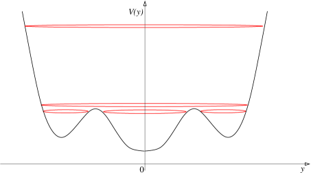
Figure 8: The effective potential for spinning string configurations resulting from two rings. A long string configuration can split into smaller strings, and smaller strings can merge into longer strings.

The splitting is characterized by the occurrence of a new zero in the quantity in expression (48), together with a maximum of the effective potential at that zero. This is new. Its effect is to give a divergence of the quantities $E$ and $S$, although the length of the string is not itself diverging. This is contrast to the divergence encountered in the long string case in the previous section which occurred for diverging length. The divergence here is for finite length, and is the characteristic of the string wishing to break into smaller strings, or join with others to make a larger one (depending upon whether one is approaching the maximum from above or below).

The origin of the divergence can be simply traced to the fact that the integrals all have the measure:

$$d\sigma=\frac{\sqrt{{\widetilde{z}}+1}}{y\sqrt{a}}\frac{dy}{\sqrt{{\cal E}-V(y)}}\ ,$$ (49)

and near the splitting point, $y_{s}$, we have:

$$V(y)={\cal E}-\frac{|V^{\prime\prime}(y_{s})|}{2}(y-y_{s})^{2}+O(y-y_{s})^{3}\ ,$$ (50)

and since the rest of the integrand in the expressions (17) for $E$ and $S$ involve no special features in the neighbourhood of the splitting point:

$$E = \frac{\sqrt{\eta}}{2\pi\alpha^{\prime}}\int^{y_{0}}dy\,\,2\cosh{G}\sqrt{\frac{1+\widetilde{z}}{\left(1+\eta+\frac{1}{\widetilde{z}}\right)}}\ ,$$

$$S = \frac{\sqrt{\eta+1}}{2\pi\alpha^{\prime}}\int^{y_{0}}dy\,\,e^{G}\sqrt{\frac{1+\widetilde{z}}{\left(1+\eta+\frac{1}{\widetilde{z}}\right)}}\ ,$$ (51)

there is always a logarithmic divergence in these quantities as $y_{0}$ (one of the turning points for a configuration) approaches the splitting point $y_{s}$ (a turning point which is also a maximum of $V(y)$).

This results in a new characteristic behaviour for $E$ vs $S$ for our operators near these points. They both diverge logarithmically as the quantity $\epsilon=y_{s}-y_{0}$ vanishes:

$$E(\epsilon)=C(\eta_{cr}+1)\ln{\frac{1}{\epsilon}}+O(\epsilon^{0})\ ,$$

$$S(\epsilon)=C\sqrt{(\eta_{cr}+1)\eta_{cr}}\ln{\frac{1}{\epsilon}}+O(\epsilon^{0})\ ,$$ (52)

where

$$C\equiv\frac{1}{\pi\alpha^{\prime}}\left.\sqrt{\frac{2(1+\widetilde{z})\widetilde{z}^{2}}{\widetilde{z}^{\prime\prime}}}\right|_{y_{s}}\ ,$$ (53)

and so we have a leading linear relation between $E$ and $S$ in the split/joint regime:

$$E=\left(\frac{\eta_{cr}+1}{\eta_{cr}}\right)^{\frac{1}{2}}S+O(S^{0})\ ,$$ (54)

where $\eta_{cr}$ is given by:

$$1+\eta_{cr}=-\frac{1}{\widetilde{z}(y_{s})}\ .$$ (55)

This is a characteristically different behaviour from the behaviour observed in the long string regime[14], showing the logarithmic behaviour of the anomalous dimension of the associated operators, presented in equation (47). It would be interesting to reproduce this behaviour in the dual gauge theory.

We plotted graphs of $E$ vs $S$ for a non–centred string in figure 9, using a three–ring example, with the radii tuned so as to produce a minimum in $V(y)$ away from $y=0$. (The three–ring example we used for this plot had $r_{0}^{(1)}=1,r_{0}^{(2)}=4$, and the third ring at a very much larger distance so as to cleanly isolate the maximum in $V(y)$.)

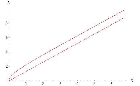
Figure 9: Plots of $E$ vs $S$ for a non–centred string including the short string regime (Regge) at low energy and the linear “splitting regime” at high energy. The upper curve is the result of numerically evaluating the quantities defined by the integrals in the text. The lower curve is a plot of the leading linear term of the analytic result of equation (54) for the splitting regime.

4 Closing Remarks

The new coordinates of ref.[1] have made it easy to study rather interesting configurations of smeared giant gravitons as spinning string backgrounds. These backgrounds allow the strings to take on more interesting behaviour than in the case of pure AdS. We were able to uncover this because we designed an ansatz for the spinning string configuration which allowed for a reduction to a simple one–dimensional mechanical system. A wide range of interesting potentials for this problem can be engineered by adjusting the size and distributions of the smeared gravitons. In particular, the fact that the potential can have multiple minima yielded a variety of new behaviours for the strings. This all translates rather straightforwardly into statements about the associated operators in the gauge theory, and it would be interesting to compare to computations within the field theory with a preparation of the corresponding background chiral primaries with large R–charge.

The description of the splitting and joining of the strings is intriguingly simple. In fact, as it reduces to the problem of studying the coalescence of branch cuts of a simple function, it is very similar in spirit to the ingredients which arise in solving some large $N$ matrix models[16]. There, a divergence occurs as the model tries to make the transition from one–cut support to multiple cuts, just as we saw here for the splitting of the string. Perhaps this connection holds some useful clues for other applications. Another interesting question is whether there is any sense to be made of quantum mechanical effects in this effective potential. Would tunneling effects between neighbouring minima correspond to new decay channels in the full type IIB background and hence in the dual gauge theory? This is also worth exploring.

Finally, the questions we mentioned in the introduction deserve to be repeated here. Are there accessible physical manifestations of an underlying reduced model (analogous to the matrix model’s fermionic phase space for this 1/2–BPS situation) in appropriate coordinates for supergravity duals of Yang–Mills theory with fewer supersymmetries? Might they serve as powerful analytical tools for a class of interesting physical questions? The intriguing way in which the coordinates of ref.[1] operate is cause for optimism.

References

- [1] H. Lin, O. Lunin, and J. Maldacena, “Bubbling AdS space and 1/2 BPS geometries,” hep-th/0409174.
- [2] D. Berenstein, “A toy model for the AdS/CFT correspondence,” JHEP 07 (2004) 018, hep-th/0403110.
- [3] J. McGreevy, L. Susskind, and N. Toumbas, “Invasion of the giant gravitons from anti-de Sitter space,” JHEP 06 (2000) 008, hep-th/0003075.
- [4] M. T. Grisaru, R. C. Myers, and O. Tafjord, “SUSY and Goliath,” JHEP 08 (2000) 040, hep-th/0008015.
- [5] A. Hashimoto, S. Hirano, and N. Itzhaki, “Large branes in AdS and their field theory dual,” JHEP 08 (2000) 051, hep-th/0008016.
- [6] A. Buchel, A. W. Peet, and J. Polchinski, “Gauge dual and noncommutative extension of an N = 2 supergravity solution,” Phys. Rev. D63 (2001) 044009, hep-th/0008076.
- [7] N. J. Evans, C. V. Johnson, and M. Petrini, “The enhançon and N = 2 gauge theory/gravity RG flows,” JHEP 10 (2000) 022, hep-th/0008081.
- [8] C. V. Johnson, K. J. Lovis, and D. C. Page, “The Kähler structure of supersymmetric holographic RG flows,” JHEP 10 (2001) 014, hep-th/0107261.
- [9] C. V. Johnson, K. J. Lovis, and D. C. Page, “Probing some N = 1 AdS/CFT RG flows,” JHEP 05 (2001) 036, hep-th/0011166.
- [10] K. Pilch and N. P. Warner, “Generalizing the N = 2 supersymmetric RG flow solution of IIB supergravity,” Nucl. Phys. B675 (2003) 99–121, hep-th/0306098.
- [11] K. Pilch and N. P. Warner, “N = 1 supersymmetric solutions of IIB supergravity from Killing spinors,” hep-th/0403005.
- [12] N. Halmagyi, K. Pilch, C. Romelsberger, and N. P. Warner, “The complex geometry of holographic flows of quiver gauge theories,” hep-th/0406147.
- [13] J. E. Carlisle and C. V. Johnson, “Holographic RG flows and universal structures on the Coulomb branch of N = 2 supersymmetric large N gauge theory,” JHEP 07 (2003) 039, hep-th/0306168.
- [14] S. S. Gubser, I. R. Klebanov, and A. M. Polyakov, “A semi-classical limit of the gauge/string correspondence,” Nucl. Phys. B636 (2002) 99–114, hep-th/0204051.
- [15] A. A. Tseytlin, “Semiclassical strings and AdS/CFT,” hep-th/0409296.
- [16] E. Brezin, C. Itzykson, G. Parisi, and J. B. Zuber, “Planar Diagrams,” Commun. Math. Phys. 59 (1978) 35.
- [17] K. Peeters, J. Plefka, and M. Zamaklar, “Splitting spinning strings in AdS/CFT,” hep-th/0410275.