Fermionic quantization and configuration spaces for the Skyrme and Faddeev-Hopf models

Abstract

The fundamental group and rational cohomology of the configuration spaces of the Skyrme and Faddeev-Hopf models are computed. Physical space is taken to be a compact oriented 3-manifold, either with or without a marked point representing an end at infinity. For the Skyrme model, the codomain is any Lie group, while for the Faddeev-Hopf model it is $S^{2}$. It is determined when the topology of configuration space permits fermionic and isospinorial quantization of the solitons of the model within generalizations of the frameworks of Finkelstein-Rubinstein and Sorkin. Fermionic quantization of Skyrmions is possible only if the target group contains a symplectic or special unitary factor, while fermionic quantization of Hopfions is always possible. Geometric interpretations of the results are given.

1 Introduction

The most straightforward procedure for quantizing a Lagrangian dynamical system with configuration space $Q$ is to specify the quantum state by a wavefunction $\psi:Q\rightarrow{\mathbb{C}}$, but many other procedures are possible [30]. One may take $\psi$ to be a section of a complex line bundle over $Q$. Clearly we recover the original quantization if the bundle is trivial. Depending on the topology of $Q$ there may be many inequivalent line bundles, giving rise to quantization ambiguity. The set of equivalence classes of line bundles is parametrized by $H^{2}(Q,{\mathbb{Z}})$. Quantization ambiguity can be used to generate fermionic or bosonic quantizations of the same classical system. The example of a charged particle under the influence of a magnetic monopole studied by Dirac [12, 13] clearly demonstrates the utility of complex line bundles for analyzing quantum dynamics. See also, the discussion in [36] and [7, chapter 6].

In the case of a Lagrangian field theory supporting topological solitons, configuration space is typically the space of (sufficiently regular) maps from some 3-manifold (representing physical space) to some target manifold. A famous example of this is the Skyrme model with target space ${\rm SU}(N)$, $N\geq 2$ and physical space ${\mathbb{R}}^{3}$. Here fermionic quantization is phenomenologically crucial since the solitons are taken to represent protons and neutrons.

Recall the distinction between bosons and fermions: a macroscopic ensemble of identical bosons behaves statistically as if aribtrarily many particles can lie in the same state, while a macroscopic ensemble of identical fermions behaves as if no two particles can lie in the same state. Photons are examples of particles with bosonic statistics and electrons are examples of particles with fermionic statistics. There are several theoretical models of particle statistics. In quantum mechanics, the wavefunction representing a multiparticle state is symmetric under exchange of any pair of identical bosons, and antisymmetric under exchange of any pair of identical fermions. In conventional perturbative quantum field theory, commuting fields are used to represent bosons and anti-commuting fields are used to represent fermions. More precisely, bosons have commuting creation operators and fermions have anti-commuting creation operators. However, there are times when fermions may arise within a field theory with purely bosonic fundamental fields. This phenomenon is called emergent fermionicity, and it relies crucially on the topological properties of the underlying configuration space of the model. Analogous instances of emergent fermionicity in quantum mechanical (rather than field theoretic) settings are described in [10, 29, 36] and [7, chapter 7].

When Skyrme originally proposed his model, it was not clear how fermionic quantization of the solitons could be achieved, a fundamental gap which he acknowledged [31]. The possibility of fermionically quantizing the Skyrme model was first demonstrated (for $N=2$) by Finkelstein and Rubinstein [15]. Full consistency of their quantization procedure was established by Giulini [16]. The case $N\geq 3$ was dealt with in a rather different way by Witten [35] at the cost of introducing a new term into the Skyrme action. This was a crucial development, since the $N=3$ model is particularly phenomenologically favoured. Although the approaches of Finkelstein-Rubinstein and Witten appear quite different, they can be treated in a common framework, as demonstrated by Sorkin [32]. See [1] and [7] for exposition about where the Skyrme model fits into modern physics. Also see [2], and [28] for a discussion of fermionic quantization of ${\rm SU}(N)$ valued Skyrme fields. We will review the Finkelstein-Rubinstein and Sorkin models of particle statistics in section 5 below, and describe the obvious generalization of their models when the domain of the soliton is something other than ${\mathbb{R}}^{3}$.

Spin is a property of a particle state associated with how it transforms under spatial rotations. Let us briefly review the usual mathematical models of spin. There are two general situations. In one, space admits a global rotational symmetry, in the other, it does not. When physical space is ${\mathbb{R}}^{3}$, so space-time is usual Minkowski space, the classical rotational symmetries induce quantum symmetries that are representations of the $Spin$ group. These irreducible representations are labeled by half integers (one half of the number of boxes in a Young diagram for a representation of SU$(2)$.) The integral representations are honest representations of the rotation group, but the fractional ones are not. The spin of a particle is the half integer labelling the ${\rm SU}(2)$ representation under which its wavefunction transforms. If the spin is not an integer, the particle is said to be spinorial. When physical space is not ${\mathbb{R}}^{3}$, one can instead consider the bundle of frames over physical space (vierbeins). Spin may then be modeled by the action of the rotation group on these frames [9]. The easiest case in this direction is when space-time admits a spin structure. This reconciliation of spin with the possibility of a curved space time was an important discovery in the last century. The situation is parallel in nonlinear models. In the easiest example of of a model with solitons incorporating spin, the configuration space is not ${\mathbb{R}}^{3}$, but maps defined on ${\mathbb{R}}^{3}$. The rotation group acts on such maps by precomposition. Sorkin described a model for the spin of solitons which generalizes to any maps defined on any domain. We cover this in section 5.

Although spin and particle statistics have completely different conceptual origins, there are strong connexions between the two. The spin-statistics theorem asserts, in the context of axiomatic quantum field theory, that particles are fermionic if and only if they are spinorial. Said differently, any particle with fractional spin is a fermion, and any particle with integral spin is a boson. Analogous spin-statistics theorems have been found for solitons also. Such a theorem was proved for ${\rm SU}(2)$ Skyrmions on ${\mathbb{R}}^{3}$ by Finkelstein and Rubinstein [15], and for arbitrary textures on ${\mathbb{R}}^{3}$ by Sorkin [32], using only the topology of configuration space. By a texture, we mean that the field must approach a constant limiting value at spatial infinity, in contrast to, say, monopoles and vortices. So pervasive is the link between fermionicity and spinoriality that the two are often elided. For example, Ramadas argued that it was possible to fermionically quantize SU$(N)$ Skyrmions on ${\mathbb{R}}^{3}$ because it was possible to spinorially quantize them [28].

Isospin is the conserved quantity analogous to spin associated with an internal rotational symmetry. As in the simplest model of spin, a particle’s isospin is a half integer labelling the representation of the quantum symmetry group corresponding to the classical internal ${\rm SO}(3)$ symmetry. In all the models we consider, the target space has a natural $SO(3)$ action, so it will make sense to determine whether these models admit isospinorial quantization in the usual sense. Krusch [24] has shown that ${\rm SU}(2)$ Skyrmions are spinorial if and only if they are isospinorial, which is in good agreement with nuclear phenomenology, since they represent bound states of nucleons. Recall that nucleon is the collective term for the proton and neutron. Both have spin and isospin 1/2 but are in different eigenstates of the 3rd component of isospin: the proton has $I_{3}=1/2$, and the neutron has $I_{3}=-1/2$. In general, the integrality of spin is unrelated to that of isospin. Strange hadrons can have half-integer spin and integer isospin (and vice-versa). For example, the $\Sigma$-baryon has isospin $1$, but spin $1/2$, and the $K$ mesons have isospin $1/2$ and spin $1$. One would hope, therefore, that the correlation found by Krusch fails in the ${\rm SU}(N)$ Skyrme model with $N>2$, since this is supposed to model low energy QCD with more than two light quark flavours, and should therefore be able to accommodate the more exotic baryons. The mathematical reader unfamiliar with spin, isospin, strangeness etc. may find the book by Halzen and Martin [18] and the comprehensive listing of particles and their properties in [26] helpful.

Emergent fermionicity, like (iso)spinoriality, can often be incorporated into a quantum system by exploiting the possibility of differences between the classical and quantum symmetries of the space of quantum states [7, chapter 7]. A spinning top is a well known example of this. The classical symmetry group is SO$(3)$, while the quantum symmetry group for some quantizations is SU$(2)$, [10, 29]. An electron in the field of a magnetic monopole is also a good example, [7, chapter 7] and [36]. We emphasize, however, that emergent fermionicity does not depend on any symmetry assumptions. In fact, the model of particle statistics that we mainly consider (Sorkin’s model) depends only on the topology of the configuration space.

The purpose of this paper is to determine the quantization ambiguity for a wide class of field theories supporting topological solitons of texture type in 3 spatial dimensions. We will allow (the one point compactification of) physical space to be any compact, oriented 3-manifold $M$ and target space to be any Lie group $G$, or the 2-sphere. The results use only the topology of configuration space and are completely independent of the dynamical details of the field theory. They cover, therefore, the Faddev-Hopf and general Skyrme models on any orientable domain. Our main mathematical results will be the computation of the fundamental group and the rational or real cohomology ring of $Q$. (The universal coefficient theorem implies that the rational dimension of the rational cohomology is equal to the real dimension of the real cohomology. Homotopy theorists tend to express results using rational coefficients and physicists tend to use real or complex coefficients.) We shall see that quantization ambiguity, as described by $H^{2}(Q,{\mathbb{Z}})$, may be reconstructed from these data. We also give geometric interpretations of the algebraic results which are useful for purposes of visualization. We then determine under what circumstances the quantization ambiguity allows for consistent fermionic quantization of Skyrmions and hopfions within the frameworks of Finkelstein-Rubinstein and Sorkin. We finally discuss the spinorial and isospinorial quantization of these models.

The main motivation for this work was to test the phenomenon of emergent fermionicity (i.e. fermionic solitons in a bosonic theory) in the Skyrme model to see, in particular, whether it survives the generalization from domain ${\mathbb{R}}^{3}$ to domain $M$. Our philosophy is that a concept in field theory which cannot be properly formulated on any oriented domain should not be considered fundamental. In fact, we shall see indications that emergent fermionicity is insensitive to the topology of $M$, but depends crucially on the topology of the target space.

We would like to thank Louis Crane, Steffen Krusch and Larry Weaver for helpful conversations about particle physics.

2 Notation and statement of results

Recall that topologically distinct complex line bundles over a topological space $Q$ are classified by $H^{2}(Q,{\mathbb{Z}})$. Note that $Q$ need have no differentiable structure to make sense of this: we can define $c_{1}(L)\in H^{2}(Q,{\mathbb{Z}})$ corresponding to bundle $L$ directly in terms of the transition functions of $L$ rather than thinking of it as the curvature of a unitary connexion on $L$ [30]. So this classification applies in the cases of interest. The free part of $H^{2}(Q,{\mathbb{Z}})$ is determined by $H^{2}(Q,{\mathbb{R}})$, while its torsion is isomorphic to the torsion of $H_{1}(Q)$. For any topological space, $H_{1}(Q)$ is isomorphic to the abelianization of $\pi_{1}(Q)$. The bundle classification problem is solved, therefore, once we know $\pi_{1}(Q)$ and $H^{2}(Q,{\mathbb{R}})$.

In this section we will define the configuration spaces that we consider, set up notation and state our main topological results. There are in fact many different but related configuration spaces that we could consider (for example spaces of free maps versus spaces of base pointed maps) and several different possibilities depending on whether the domain is connected etc. We give clean statements of our results for special cases in this section, and describe how to obtain the most general results in the next section. The next section will also include some specific examples. Of course homotopy theorists have studied the algebraic topology of spaces of maps. The paper by Federer gives a spectral sequence whose limit group is a sum of composition factors of homotopy groups for a space of based maps [14]. We do not need a way to compute – we actually need the computations, and this is what is contained here.

Let $M$ be a compact, oriented 3-manifold and $G$ be any Lie group. Then the first configuration space we consider is either ${\mbox{FreeMaps}}(M,G)$, the space of continuous maps $M\rightarrow G$, or $G^{M}$, the subset of ${\mbox{FreeMaps}}(M,G)$ consisting of those maps which send a chosen basepoint $x_{0}\in M$ to $1\in G$. We will address configuration spaces of $S^{2}$-valued maps later in this section and paper. Both ${\mbox{FreeMaps}}(M,G)$ and $G^{M}$ are given the compact open topology. In practice some Sobolev topology depending on the energy functional is probably appropriate. The issue of checking the algebraic topology arguments given in this paper for classes of Sobolev maps is interesting. See [6] for a discussion of the correct setting and arguments generalizing the labels of the path components of these configuration spaces for Sobolev maps. The space ${\mbox{FreeMaps}}(M,G)$ is appropriate to the $G$-valued Skyrme model on a genuinely compact domain, while $G^{M}$ is appropriate to the case where physical space $\hat{M}$ is noncompact but has a connected end at infinity which, for finite energy maps, may be regarded as a single point $x_{0}$ in the one point compactification $M$ of $\hat{M}$.

The space $G^{M}$ splits into disjoint path components which are labeled by certain cohomology classes on $M$ [4]. Let $(G^{M})_{0}$ be the identity component of the topological group $G^{M}$, that is, the path component containing the constant map $u(x)=1$. In physical terms $(G^{M})_{0}$ is the vacuum sector of the model. Then $(G^{M})_{0}$ is a normal subgroup of $G^{M}$ whose cosets are precisely the other path components. The set of path components itself has a natural group structure. As a set, the space of path components of the based maps is given by the following proposition.

Proposition 1 (Auckly-Kapitanski)

Let $G$ be a compact, connected Lie group and $M$ be a connected, closed $3$-manifold. The set of path components of $G^{M}$ is

$$G^{M}/(G^{M})_{0}\,\cong\,H^{3}(M;\pi_{3}(G))\times H^{1}(M;H_{1}(G)).$$

The reason the above proposition only describes the set of path components is that Auckly and Kapitanski only establish an exact sequence

$$0\to H^{3}(M;\pi_{3}(G))\to G^{M}/(G^{M})_{0}\to H^{1}(M;H_{1}(G))\to 0.$$

To understand the group structure on the set of path components one would have to understand a bit more about this sequence (e.g. does it split?). Every path component of $G^{M}$ is homeomorphic to $(G^{M})_{0}$ since $\widetilde{u}(x)\mapsto u(x)^{-1}\widetilde{u}(x)$ is a homeomorphism $u\,(G^{M})_{0}\rightarrow(G^{M})_{0}$. Our first result computes the fundamental group of the configuration space of based $G$-valued maps.

Theorem 2

If $M$ is a closed, connected, orientable $3$-manifold, and $G$ is any Lie group, then

$$\pi_{1}(G^{M})\,\cong\,{\mathbb{Z}}_{2}^{s}\,\oplus H^{2}(M;\pi_{3}(G)).$$

Here $s$ is the number of symplectic factors in the lie algebra of $G$.

Our next result gives the whole real cohomology ring $H^{*}((G^{M})_{0},{\mathbb{R}})$, including its multiplicative structure. This, of course, includes the required computation of $H^{2}((G^{M})_{0},{\mathbb{R}})$.

Similarly to Yang-Mills theory, there is a $\mu$ map,

$$\mu:H_{d}(M;{\mathbb{R}})\otimes H^{j}(G;{\mathbb{R}})\to H^{j-d}(G^{M};{\mathbb{R}}),$$

and the cohomology ring is generated (as an algebra) by the images of this map. To state the theorem we do not need the definition of this $\mu$ map, but the definition may be found in subsection 4.3 of section 4, in particular, equation (4.1).

Theorem 3

Let $G$ be a compact, simply-connected, simple Lie group. The cohomology ring of any of these groups is a free graded-commutative unital algebra over ${\mathbb{R}}$ generated by degree $k$ elements $x_{k}$ for certain values of $k$ (and with at most one exception at most one generator for any given degree). The values of $k$ depend on the group and are listed in table 1 in section 3. Let $M$ be a closed, connected, orientable $3$-manifold. The cohomology ring $H^{*}((G^{M})_{0};{\mathbb{R}})$ is the free graded-commutative unital algebra over ${\mathbb{R}}$ generated by the elements $\mu(\Sigma_{j}^{d}\otimes x_{k})$, where $\Sigma_{j}^{d}$ form a basis for $H_{d}(M;{\mathbb{R}})$ for $d>0$ and $k-d>0$.

The examples in the next section best illuminate the details of the above theorem.

Turning to the Faddeev-Hopf model, the configuration space of interest is either the space of free $S^{2}$-valued maps ${\mbox{FreeMaps}}(M,S^{2})$, or $(S^{2})^{M}$, the space of based continuous maps $M\rightarrow S^{2}$. One can analyze ${\mbox{FreeMaps}}(M,S^{2})$ in terms of $(S^{2})^{M}$ by making use of the natural fibration

$$(S^{2})^{M}\hookrightarrow{\mbox{FreeMaps}}(M,S^{2})\stackrel{{\scriptstyle\pi}}{{\rightarrow}}S^{2},\qquad\pi:u(x)\mapsto u(x_{0}).$$

The fundamental cohomology class (orientation class), $\mu_{S^{2}}\in H^{2}(S^{2},{\mathbb{Z}})$ plays an important role in the description of the mapping spaces of $S^{2}$-valued maps. The path components of $(S^{2})^{M}$ were determined by Pontrjagin [27]:

Theorem 4 (Pontrjagin)

Let $M$ be a closed, connected, oriented 3-manifold, and $\mu_{S^{2}}$ be a generator of $H^{2}(S^{2};{\mathbb{Z}})\cong{\mathbb{Z}}$. To any based map $\varphi$ from $M$ to $S^{2}$ one may associate the cohomology class, $\varphi^{*}\mu_{S^{2}}\in H^{2}(M;{\mathbb{Z}})$. Every second cohomology class may be obtained from some map and any two maps with different cohomology classes lie in distinct path components of $(S^{2})^{M}$. Furthermore, the set of path components corresponding to a cohomology class, $\alpha\in H^{2}(M)$ is in bijective correspondence with $H^{3}(M)/(2\alpha\smallsmile H^{1}(M))$.

A discussion of this theorem in the setting of the Faddeev model may be found in [5] and [6]. Let $(S^{2})^{M}_{0}$ denote the vacuum sector, that is the path component of the constant map, and $(S^{2})^{M}_{\varphi}$ denote the path component containing $\varphi$. Since $(S^{2})^{M}$ is not a topological group, there is no reason to expect all its path components to be homeomorphic. We will prove, however that two components $(S^{2})^{M}_{\varphi}$ and $(S^{2})^{M}_{\psi}$ are homeomorphic if $\varphi^{*}\mu_{S^{2}}=\psi^{*}\mu_{S^{2}}$:

Theorem 5

Let $\varphi\in(S^{2})^{M}$ such that $\varphi^{*}\mu_{S^{2}}=\psi^{*}\mu_{S^{2}}$. Then $(S^{2})^{M}_{\varphi}\cong(S^{2})^{M}_{\psi}$.

Moreover, the fundamental group of any component can be computed, as follows.

Theorem 6

Let $M$ be closed, connected and orientable. For any $\varphi\in(S^{2})^{M}$, the fundamental group of $(S^{2})^{M}_{\varphi}$ is given by

$$\pi_{1}((S^{2})^{M}_{\varphi})\cong{\mathbb{Z}}_{2}\oplus H^{2}(M;{\mathbb{Z}})\oplus\hbox{\rm ker}(2\varphi^{*}\mu_{S^{2}}\smallsmile).$$

Here $2\varphi^{*}\mu_{S^{2}}\smallsmile:H^{1}(M;{\mathbb{Z}})\to H^{3}(M;{\mathbb{Z}})$ is the usual map given by the cup product.

There is a general relationship between the fundamental group of the configuration space of based $S^{2}$-valued maps and the corresponding configuration space of free maps. It implies the following result for the fundamental group of the space of free $S^{2}$-valued maps.

Theorem 7

We have $\pi_{1}({\mbox{FreeMaps}}(M,S^{2})_{\varphi})\cong{\mathbb{Z}}_{2}\oplus\left(H^{2}(M;{\mathbb{Z}})/\langle 2\varphi\mu_{S^{2}}\rangle\right)\oplus\hbox{\rm ker}(2\varphi^{*}\mu_{S^{2}}\smallsmile)$.

To complete the classification of complex line bundles over $(S^{2})^{M}_{\varphi}$ one also needs the second cohomology $H^{2}((S^{2})^{M}_{\varphi};{\mathbb{R}})$, which can be extracted from the above theorem and the following computation of the cohomology ring $H^{*}((S^{2})^{M}_{\varphi},{\mathbb{R}})$:

Theorem 8

Let $M$ be closed, connected and orientable, let $\varphi:M\to S^{2}$, let $\Sigma_{j}^{d}$ form a basis for $H_{d}(M;{\mathbb{R}})$ for $d<3$, and let $\{\alpha_{k}\}$ for a basis for $\hbox{ker}(2\varphi^{*}\mu_{S^{2}}\cup):H^{1}(M;{\mathbb{Z}})\to H^{3}(M;{\mathbb{Z}}))$. The cohomology ring $H^{*}((S^{2})^{M}_{\varphi};{\mathbb{R}})$ is the free graded-commutative unital algebra over ${\mathbb{R}}$ generated by the elements $\alpha_{k}$ and $\mu(\Sigma_{j}^{d}\otimes x)$, where $x\in H^{3}(Sp_{1};{\mathbb{Z}})$ is the orientation class. The classes $\alpha_{k}$ have degree $1$ and $\mu(\Sigma_{j}^{d}\otimes x)$ have degree $3-d$.

We can compute the cohomology of the space of free $S^{2}$-valued maps using the following theorem.

Theorem 9

There is a spectral sequence with $E_{2}^{p,q}=H^{p}(S^{2};{\mathbb{R}})\otimes H^{q}((S^{2})^{M}_{\varphi};{\mathbb{R}})$ converging to $H^{*}({\mbox{FreeMaps}}(M,S^{2})_{\varphi};{\mathbb{R}})$. The second differential is given by $d_{2}\mu(\Sigma^{(2)}\otimes x)=2\varphi^{*}\mu_{S^{2}}[\Sigma]\mu_{S^{2}}$ with $d_{2}$ of any other generator trivial. All higher differentials are trivial as well.

In order to compare the classical and quantum isospin symmetries, we will use the following theorem due to Gottlieb [17]. It is based on earlier work of Hattori and Yoshida [19].

Theorem 10 (Gottlieb)

Let $L\to X$ be a complex line bundle over a locally compact space. An action of a compact connected lie group on $X$, say $\rho:X\times G\to X$, lifts to a bundle action on $L$ if and only if two obstructions vanish. The first obstruction is the pull back of the first chern class, $L_{x_{0}}^{*}c_{1}(L)\in H^{2}(G;{\mathbb{Z}})$. Here $L_{x_{0}}$ is the map induced by applying the group action to the base point. The second obstruction lives in $H^{1}(X;H^{1}(G;{\mathbb{Z}}))$.

We have taken the liberty of radically changing the notation from the original theorem, and we have only stated the result for line bundles. The actual theorem is stated for principal torus bundles. Since our configuration spaces are not locally compact, we should point out that we will use one direction of this theorem by restricting to a locally compact equivariant subset. In the other direction, we will just outline a construction of the lifted action.

Our main physical conclusions are:

C1

In these models, there is a portion of quantization ambiguity that depends only on the codomain and is completely independent of the topology of the domain. This allows for the possibility that emergent fermionicity may only depend on the target.

C2

It is possible to quantize $G$-valued solitons fermionically (with odd exhange statistics) if and only if the Lie algebra contains a symplectic ($C_{n}$) or special unitary ($A_{n}$) factor.

C3

It is possible to quantize $G$-valued solitons with fractional isospin when the Lie algebra of $G$ contains a symplectic ($C_{n}$) or special unitary ($A_{n}$) factor.

C4

It is not possible to quantize $G$-valued solitons with fractional isospin when the Lie algebra does not contain such a factor.

C5

It is always possible to choose a quantization of these systems with integral isospin (however such might not be consistent with other constraints on the model)

C6

It is always possible to quantize $S^{2}$-valued solitons with fractional isospin and odd exchange statistics.

The rest of this paper is structured as follows. In section 3 we describe how to reduce the description of the topology of general $G$-valued and $S^{2}$-valued mapping spaces to the theorems listed in this section. We also provide several illustrative examples. In section 4 we review the Pontrjagin-Thom construction and describe geometric interpretations of some of our results using the Pontrjagin-Thom construction. Physical applications, particularly the possibility of consistent fermionic quantization of Skyrmions, are discussed in section 5. Finally, section 6 contains the proofs of our results.

3 Preliminary reductions and examples

We begin this section with a collection of observations that allow one to reduce questions about the topology of various mapping spaces of $G$-valued and $S^{2}$-valued maps to the theorems listed in the previous section. Many of these observations will reduce a more general mapping space to a product of special mapping spaces, or put such spaces into fibrations. These reductions ensure that our results are valid for arbitrary closed, orientable $3$-manifolds, and valid for any Lie group.

It follows directly from the definition of $\pi_{1}$ that $\pi_{1}(X\times Y)\cong\pi_{1}(X)\times\pi_{1}(Y)$. The cohomology of a product is described by the Künneth theorem, see [33]. For real coefficients it takes the simple form, $H^{*}(X\times Y)\cong H^{*}(X)\otimes H^{*}(Y)$. The cohomology ring of a disjoint union of spaces is the direct sum of the corresponding cohomology rings, i. e. $H^{*}({\perp\!\!\!\perp}X_{\nu};A)=\bigoplus H^{*}(X_{\nu};A)$. Recall that a fibration is a map with the covering homotopy property, see for example [33]. Given a fibration $F\hookrightarrow E\rightarrow B$, there is an induced long exact sequence of homotopy groups, $\dots\rightarrow\pi_{k+1}(B)\rightarrow\pi_{k}(F)\rightarrow\pi_{k}(E)\rightarrow\pi_{k}(B)\rightarrow\dots$, see [33]. By itself this sequence is not enough to determine the fundamental group of a term in a fibration from the other terms. However, combined with a bit of information about the twisting in the bundle it will be enough information. One can also relate the cohomology rings of the terms in a fibration. This is accomplished by the Serre spectral sequence, see [33].

Reduction 1

We have, ${\mbox{FreeMaps}}({\perp\!\!\!\perp}X_{\nu},Y)\cong\prod{\mbox{FreeMaps}}(X_{\nu},Y)$ and $Y^{{\perp\!\!\!\perp}X_{\nu}}\cong Y^{X_{0}}\times\prod_{\nu\neq 0}{\mbox{FreeMaps}}(X_{\nu},Y)$ where $X_{0}$ is the component of $X$ containing the base point.

It follows that there is no loss of generality in assuming that $M$ is connected. Likewise there is no loss of generality in assuming that the target is connected because of the following reduction.

Reduction 2

We have, ${\mbox{FreeMaps}}(X,{\perp\!\!\!\perp}Y_{\nu})\cong{\perp\!\!\!\perp}{\mbox{FreeMaps}}(X,Y_{\nu})$ and assuming $X$ is connected $Y^{X}=Y_{0}^{X}$ where $Y_{0}$ is the component containing the base point.

Both ${\mbox{FreeMaps}}(M,G)$ and $G^{M}$ are topological groups under pointwise multiplication. In fact ${\mbox{FreeMaps}}(M,G)\cong G^{M}\rtimes G$, the isomorphism being $u(x)\mapsto(u(x)u(x_{0})^{-1},u(x_{0}))$, which is clearly a homeomorphism ${\mbox{FreeMaps}}(M,G)\rightarrow G^{M}\times G.$ It is thus straightforward to deduce $\pi_{1}({\mbox{FreeMaps}}(M,G)$ and $H^{*}({\mbox{FreeMaps}}(M,G),{\mathbb{R}})$ from $\pi_{1}(G^{M})$ and $H^{*}(G^{M},{\mathbb{Z}})$. Note that the based case includes the standard choice $\hat{M}={\mathbb{R}}^{3}$.

Reduction 3

We have ${\mbox{FreeMaps}}(M,G)\cong G^{M}\times G$.

In the same way, we can reduce the free maps case to the based case for $S^{2}$-valued maps. In this case we only obtain a fibration. See Lemmas 18, 20 and 21.

Reduction 4

We have a fibration, $(S^{2})^{M}\hookrightarrow{\mbox{FreeMaps}}(M,S^{2})\rightarrow S^{2}$, $\pi_{0}({\mbox{FreeMaps}}(M,S^{2}))=\pi_{0}((S^{2})^{M})$, and $\pi_{1}({\mbox{FreeMaps}}(M,S^{2})_{\varphi})=\pi_{1}((S^{2})^{M}_{\varphi})$.

The relevant information about the twisting in this fibration as far as the fundamental group detects is given in the proof of Theorem 7 contained in subsection 6.3. For cohomology, the information is encoded in the second differential of the associated spectral sequence. Returning to the case of group-valued maps we know by the Cartan-Malcev-Iwasawa theorem that any connected Lie group is homeomorphic to a product $G=K\times{\mathbb{R}}^{n}$, where $K$ is compact [22].

Reduction 5

If $X^{\prime}$ and $Y^{\prime}$ are homotopy equivalent to $X$ and $Y$ respectively, then $(Y^{\prime})^{X^{\prime}}$ is homotopy equivalent to $Y^{X}$. In particular we have $G^{M}\simeq K^{M}$.

Recall that every path component of $G^{M}$ is homeomorphic to $(G^{M})_{0}$ We may therefore consider only the vacuum sector $(G^{M})_{0}$, without loss of generality. We shall see that things are very different for the Faddeev-Hopf configuration space, where we must keep track of which path component we are studying.

Reduction 6

If $G$ is a Lie group, $\tilde{G}$ is the universal covering group of its identity component and $M$ is a $3$-manifold, then

$$(\tilde{G}^{M})_{0}\cong(G^{M})_{0}.$$

Proof: Without loss of generality we may assume that $G$ is connected. We have the exact sequence,

$$1\to\tilde{G}^{M}\to G^{M}\to H^{1}(M;H_{1}(G))\to 0,$$

from [4]. The exactness follows from the unique path lifting property of covers at the first term, the lifting criteria for maps to the universal cover at the center term, and induction on the skeleton of $M$ at the last term. Clearly, the identity component of $\tilde{G}^{M}$ maps to the identity component of $G^{M}$. By the above sequence, this map is injective. Any element of $(G^{M})_{0}$, say $u$, maps to $0$ in $H^{1}(M;H_{1}(G))$, so is the image of some map in $\tilde{G}^{M}$, say $\tilde{u}$. Using the homotopy lifting property of covering spaces, we may lift the homotopy of $u$ to a constant map, to a homotopy of $\tilde{u}$ to a constant map and conclude that $\tilde{u}\in(\tilde{G}^{M})_{0}$. It follows that the map, $(\tilde{G}^{M})_{0}\to(G^{M})_{0}$ is a homeomorphism. $\Box$

Reduction 7

The universal covering group of any compact Lie group is a product of ${\mathbb{R}}^{m}$ with a finite number of compact, simple, simply-connected factors [25]. Furthermore, $\left(\prod Y_{\nu}\right)^{X}\cong\prod Y_{\nu}^{X}$ and ${\mbox{FreeMaps}}(X,\prod Y_{\nu}))\cong\prod{\mbox{FreeMaps}}(X,Y_{\nu})$.

We have therefore reduced to the case of closed, connected, orientable $M$ and compact, simple, simply-connected Lie groups. All compact, simple, simply-connected Lie groups are listed together with their center and rational cohomology in table 1.

group, $G$	center, $Z(G)$	$H^{*}(G;{\mathbb{Q}})$
$A_{n}=\hbox{SU}(n+1)$, $n\geq 2$	${\mathbb{Z}}_{n+1}$	${\mathbb{Q}}[x_{3},x_{5},\dots x_{2n+1}]$
$B_{n}=\hbox{Spin}(2n+1)$, $n\geq 3$	${\mathbb{Z}}_{2}$	${\mathbb{Q}}[x_{3},x_{7},\dots x_{4n-1}]$
$C_{n}=\hbox{Sp}(n)$, $n\geq 1$	${\mathbb{Z}}_{2}$	${\mathbb{Q}}[x_{3},x_{7},\dots x_{4n-1}]$
$D_{n}=\hbox{Spin}(2n)$, $n\geq 4$	${\mathbb{Z}}_{2}\oplus{\mathbb{Z}}_{2}$ for $n\equiv_{2}0$	${\mathbb{Q}}[x_{3},x_{7},\dots x_{4n-5},y_{2n-1}]$
	${\mathbb{Z}}_{4}$ for $n\equiv_{2}1$
$E_{6}$	${\mathbb{Z}}_{3}$	${\mathbb{Q}}[x_{3},x_{9},x_{11},x_{15},x_{17},x_{23}]$
$E_{7}$	${\mathbb{Z}}_{2}$	${\mathbb{Q}}[x_{3},x_{11},x_{15},x_{19},x_{23},x_{27},x_{35}]$
$E_{8}$	0	${\mathbb{Q}}[x_{3},x_{15},x_{23},x_{27},x_{35},x_{39},x_{47},x_{59}]$
$F_{4}$	0	${\mathbb{Q}}[x_{3},x_{11},x_{15},x_{23}]$
$G_{2}$	0	${\mathbb{Q}}[x_{3},x_{11}]$

Table 1: Simple groups

Recall from Proposition 1 that the path components of a configuration space of group-valued maps depend on the fundamental group of the group. The fundamental group of any Lie group is a discrete subgroup of the center of the universal covering group. The center of such a group is just the product of the centers of the factors.

Some comments about table 1 are in order at this point. The last generator of the cohomology ring of $D_{n}$ is labeled with a $y$ instead of an $x$ because there are two generators in degree $2n-1$ when $n$ is even. As usual, $\hbox{SU}(k)$ is the set of special unitary matrices, that is complex matrices with unit determinant satisfying, $A^{*}A=I$. The symplectic groups, $\hbox{Sp}(k)$, consist of the quaternionic matrices satisfying $A^{*}A=I$, and the special orthogonal groups, $\hbox{SO}(k)$ consist of the real matrices with unit determinant satisfying $A^{*}A=I$. The spin groups, $\hbox{Spin}(k)$ are the universal covering groups of the special orthogonal groups. The definitions of the exceptional groups may be found in [3]. The following isomorphisms hold, $\hbox{SU}(2)\cong\hbox{Sp}(1)\cong\hbox{Spin}(3)$, $\hbox{Spin}(5)\cong\hbox{Sp}(2)$, and $\hbox{Spin}(6)\cong\hbox{SU}(4)$, [3]. We will need some homotopy groups of Lie groups. Recall that the higher homotopy groups of a space are isomorphic to the higher homotopy groups of the universal cover of the space, and the higher homotopy groups take products to products. We have $\pi_{3}(G)\cong{\mathbb{Z}}$ for any of the simple $G$, and $\pi_{4}(\hbox{Sp}(n))\cong{\mathbb{Z}}_{2}$ and $\pi_{4}(G)=0$ for all other simple groups [25]. This is the reason we grouped the simple groups as we did. Note in particular that we are calling SU$(2)$ a symplectic group.

3.1 Examples

In this subsection, we present two examples that suffice to illustrate all seven reductions described earlier.

Example 1 For our first example, we take $M=(S^{2}\times S^{1}){\perp\!\!\!\perp}{\mathbb{R}{{P}}}^{3}$ and

$$G=\hbox{Sp}(2)\times\left\{\left(\begin{array}[]{cc}a&b\\ 0&c\end{array}\right)\in\hbox{GL}_{2}{\mathbb{R}}\right\}.$$

We take $((1,0,0),(1,0))\in S^{2}\times S^{1}$ as the base point in $M$. In this example, neither the domain nor codomain is connected ($G/G_{0}\cong{\mathbb{Z}}_{2}\times{\mathbb{Z}}_{2}$). In addition, the group is not reductive. We also see exactly what is meant by the number of symplectic factors in the Lie algebra: it is just the number of $C_{n}$ factors in the Lie algebra of the maximal compact subgroup of the identity component of $G$. This example requires Reductions 1, 2, 3, and 5. To analyze the topology of the spaces of free and based maps, it suffices to understand maps from $S^{2}\times S^{1}$ and ${\mathbb{R}{{P}}}^{2}$ into the identity component, $G_{0}$ (Reductions 1, 2 and 3). In fact, we may replace $G_{0}$ with $\hbox{Sp}(2)$ (Reduction 5). Proposition 1 implies that $\pi_{0}(\hbox{Sp}(2)^{S^{2}\times S^{1}})={\mathbb{Z}}$ and $\pi_{0}(\hbox{Sp}(2)^{{\mathbb{R}{{P}}}^{3}})={\mathbb{Z}}$, so $\pi_{0}({\mbox{FreeMaps}}(M,G))={\mathbb{Z}}_{2}^{4}\times{\mathbb{Z}}^{2}$ and $\pi_{0}(G^{M})={\mathbb{Z}}_{2}^{2}\times{\mathbb{Z}}^{2}$. Similarly, Theorem 2 implies that $\pi_{1}(\hbox{Sp}(2)^{S^{2}\times S^{1}})={\mathbb{Z}}_{2}\oplus{\mathbb{Z}}$ and $\pi_{1}(\hbox{Sp}(2)^{{\mathbb{R}{{P}}}^{3}})={\mathbb{Z}}_{2}\oplus{\mathbb{Z}}_{2}$, so $\pi_{1}({\mbox{FreeMaps}}(M,G))=\pi_{1}(G^{M})={\mathbb{Z}}_{2}^{3}\oplus{\mathbb{Z}}$.

Turning to the cohomology, we know that $H^{*}(\hbox{Sp}(2);{\mathbb{R}})$ is the free graded-commutative unital algebra generated by $x_{3}$ and $x_{7}$. Graded-commutative means $xy=(-1)^{|x||y|}yx$. It follows that any term with repeated factors is zero. We can list the generators of the groups in each degree. In the expression below we list the generators left to right from degree $0$ with each degree separated by vertical lines:

$$H^{*}(\hbox{Sp}(2);{\mathbb{R}})=|1|0|0|x_{3}|0|0|0|x_{7}|0|0|x_{3}x_{7}|.$$

The product structure is apparent. Theorem 3 tells us that $H^{*}((\hbox{Sp}(2))^{S^{2}\times S^{1}}_{0};{\mathbb{R}})$ is the free unital graded-commutative algebra generated by $\mu([S^{2}\times\hbox{pt}]\otimes x_{3})^{(1)}$, $\mu([\hbox{pt}\times S^{1}]\otimes x_{3})^{(2)}$, $\mu([S^{2}\times S^{1}]\otimes x_{7})^{(4)}$, $\mu([S^{2}\times\hbox{pt}]\otimes x_{7})^{(5)}$, and $\mu([\hbox{pt}\times S^{1}]\otimes x_{7})^{(6)}$. Here we have included the degree of the generator as a subscript. In the same way we see that $H^{*}((\hbox{Sp}(2))^{{\mathbb{R}{{P}}}^{3}}_{0};{\mathbb{R}})$ is the free unital graded-commutative algebra (FUGCA) generated by $\mu([{\mathbb{R}{{P}}}^{3}]\otimes x_{7})^{(4)}$. Using the reductions and the Künneth theorem we see that $H^{*}((G^{M})_{0};{\mathbb{R}})$ is the FUGCA generated by $\mu([S^{2}\times\hbox{pt}]\otimes x_{3})^{(1)}$, $\mu([\hbox{pt}\times S^{1}]\otimes x_{3})^{(2)}$, $x_{3}$, $\mu([S^{2}\times S^{1}]\otimes x_{7})^{(4)}$, $\mu([{\mathbb{R}{{P}}}^{3}]\otimes x_{7})^{(4)}$, $\mu([S^{2}\times\hbox{pt}]\otimes x_{7})^{(5)}$, $\mu([\hbox{pt}\times S^{1}]\otimes x_{7})^{(6)}$, $x_{7}$. Notice that this is not finitely generated as a vector space even though it is finitely generated as an algebra. This is because it is possible to have repeated even degree factors. The vector space in each degree is still finite dimensional.

The cohomology ring of the configuration space of based loops is just the direct sum, $H^{*}(G^{M};{\mathbb{R}})=\bigoplus_{\pi_{0}(G^{M})}H^{*}((G^{M})_{0};{\mathbb{R}})$. Notice that it is infinitely generated as an algebra. The cohomology of the identity component will usually be the important thing. Using the reductions, we see that the identity component of the space of free maps is up to homotopy just the product, ${\mbox{FreeMaps}}(M,G)_{0}=G^{M}\times\hbox{Sp}(2)$, so the cohomology ring $H^{*}({\mbox{FreeMaps}}(M,G)_{0};{\mathbb{R}})$ is obtained from $H^{*}((G^{M})_{0};{\mathbb{R}})$ by adjoining new generators in degrees $3$ and $7$, say $y_{3}$ and $y_{7}$. Thus $H^{2}((G^{M})_{0};{\mathbb{Z}})\cong H^{2}({\mbox{FreeMaps}}(M,G)_{0};{\mathbb{Z}})\cong{\mathbb{Z}}\oplus{\mathbb{Z}}_{2}^{3}$.

Example 2 For this example, we take $M=T^{3}\#L(m,1)$, $G_{1}=\hbox{SO}(8)$ and $G=\hbox{U}(2)\times\hbox{SO}(8)$. Recall that the lens space $L(m,1)$ is the quotient $\hbox{Sp}(1)/{\mathbb{Z}}_{m}$ where we view ${\mathbb{Z}}_{m}$ as the $m$-th roots of unity in $S^{1}\subset\hbox{Sp}(1)$. In this example we will need to use Reductions 6 and 7. The unitary group is isomorphic to $\hbox{Sp}(1)\times_{{\mathbb{Z}}_{2}}S^{1}$, where ${\mathbb{Z}}_{2}$ is viewed as the diagonal subgroup, $\pm(1,1)$. The universal covering group of SO$(8)$ is Spin$(8)$. It follows that $G_{1}$ and $G$ are connected, $G$ has universal covering group $\hbox{Sp}(1)\times{\mathbb{R}}\times\hbox{Spin}(8)$, and fundamental groups are $\pi_{1}(\hbox{Spin}(8))={\mathbb{Z}}_{2}$ and $\pi_{1}(G)={\mathbb{Z}}\oplus{\mathbb{Z}}_{2}$. The group $G$ has two simple factors, one of which is symplectic. The integral cohomology of $M$ is given by $H^{1}(M;{\mathbb{Z}})\cong{\mathbb{Z}}^{3}$ and $H^{2}(M;{\mathbb{Z}})\cong{\mathbb{Z}}^{3}\oplus{\mathbb{Z}}_{m}$. The universal coefficient theorem and Proposition 1 imply $\pi_{0}(G_{1}^{M})=\pi_{0}({\mbox{FreeMaps}}(M,G_{1}))={\mathbb{Z}}\times{\mathbb{Z}}_{2}^{4}$ if $m$ is even, ${\mathbb{Z}}\times{\mathbb{Z}}_{2}^{3}$ if $m$ is odd, and $\pi_{0}(G^{M})=\pi_{0}({\mbox{FreeMaps}}(M,G))={\mathbb{Z}}^{5}\times{\mathbb{Z}}_{2}^{4}$ if $m$ is even and ${\mathbb{Z}}^{5}\times{\mathbb{Z}}_{2}^{3}$ if $m$ is odd. Theorem 2 implies that $\pi_{1}(G_{1}^{M})={\mathbb{Z}}^{3}\oplus{\mathbb{Z}}_{m}$, $\pi_{1}({\mbox{FreeMaps}}(M,G_{1}))={\mathbb{Z}}^{3}\oplus{\mathbb{Z}}_{m}\oplus{\mathbb{Z}}_{2}$, $\pi_{1}(G^{M})={\mathbb{Z}}^{6}\oplus{\mathbb{Z}}_{m}^{2}\oplus{\mathbb{Z}}_{2}$ and $\pi_{1}({\mbox{FreeMaps}}(M,G))={\mathbb{Z}}^{7}\oplus{\mathbb{Z}}_{m}^{2}\oplus{\mathbb{Z}}_{2}^{2}$.

Turning once again to cohomology, we see from Theorem 3 that $H^{*}((\hbox{U}(2)^{M})_{0};{\mathbb{R}})$ is the FUGCA generated by $\mu([T^{2}\times\hbox{pt}]\otimes x_{3})^{(1)}$, $\mu([S^{1}\times\hbox{pt}\times S^{1}]\otimes x_{3})^{(1)}$, $\mu([\hbox{pt}\times T^{2}]\otimes x_{3})^{(1)}$, $\mu([S^{1}\times\hbox{pt}]\otimes x_{3})^{(2)}$, $\mu([\hbox{pt}\times S^{1}\hbox{pt}]\otimes x_{3})^{(2)}$, and $\mu([\hbox{pt}\times S^{1}]\otimes x_{3})^{(2)}$.

Also, $H^{*}((G_{1}^{M})_{0};{\mathbb{R}})$ is the FUGCA generated by $\mu([T^{2}\times\hbox{pt}]\otimes y_{3})^{(1)}$, $\mu([S^{1}\times\hbox{pt}\times S^{1}]\otimes y_{3})^{(1)}$, $\mu([\hbox{pt}\times T^{2}]\otimes y_{3})^{(1)}$, $\mu([S^{1}\times\hbox{pt}]\otimes y_{3})^{(2)}$, $\mu([\hbox{pt}\times S^{1}\hbox{pt}]\otimes y_{3})^{(2)}$, $\mu([\hbox{pt}\times S^{1}]\otimes y_{3})^{(2)}$, $\mu([T^{3}]\otimes y_{7})^{(4)}$, $\mu([T^{3}]\otimes z_{7})^{(4)}$, $\mu([T^{2}\times\hbox{pt}]\otimes y_{7})^{(5)}$, $\mu([S^{1}\times\hbox{pt}\times S^{1}]\otimes y_{7})^{(5)}$, $\mu([\hbox{pt}\times T^{2}]\otimes y_{7})^{(5)}$, $\mu([S^{1}\times\hbox{pt}]\otimes y_{7})^{(6)}$, $\mu([\hbox{pt}\times S^{1}\hbox{pt}]\otimes y_{7})^{(6)}$, $\mu([\hbox{pt}\times S^{1}]\otimes y_{7})^{(6)}$, $\mu([T^{2}\times\hbox{pt}]\otimes z_{7})^{(5)}$, $\mu([S^{1}\times\hbox{pt}\times S^{1}]\otimes z_{7})^{(5)}$, $\mu([\hbox{pt}\times T^{2}]\otimes z_{7})^{(5)}$, $\mu([S^{1}\times\hbox{pt}]\otimes z_{7})^{(6)}$, $\mu([\hbox{pt}\times S^{1}\hbox{pt}]\otimes z_{7})^{(6)}$, $\mu([\hbox{pt}\times S^{1}]\otimes z_{7})^{(6)}$, $\mu([T^{3}]\otimes y_{11})^{(8)}$, $\mu([T^{2}\times\hbox{pt}]\otimes y_{11})^{(9)}$, $\mu([S^{1}\times\hbox{pt}\times S^{1}]\otimes y_{11})^{(9)}$, $\mu([\hbox{pt}\times T^{2}]\otimes y_{11})^{(9)}$, $\mu([S^{1}\times\hbox{pt}]\otimes y_{11})^{(10)}$, $\mu([\hbox{pt}\times S^{1}\hbox{pt}]\otimes y_{11})^{(10)}$, and $\mu([\hbox{pt}\times S^{1}]\otimes y_{11})^{(10)}$.

Therefore, $H^{*}((G^{M})_{0};{\mathbb{R}})$ is the FUGCA generated by all of the generators listed for the two previous algebras. We changed the notation for the generators of the cohomology of the lie groups as needed. To get to the cohomology of the identity component of the space of free maps, we would just have to add generators for the cohomology of the group $G_{0}$ to this list. In general the cohomology of a connected lie group is the same as the cohomology of the maximal compact subgroup, and every compact Lie group has a finite cover that is a product of simple, simply-connected, compact Lie groups and a torus. In this case, we need to add generators, $t_{1}$, $u_{3}$, $w_{3}$, $u_{7}$, $v_{7}$, and $u_{11}$.

Thus, $H^{2}((G_{1}^{M})_{0};{\mathbb{Z}})\cong{\mathbb{Z}}^{6}\oplus{\mathbb{Z}}_{m}$, $H^{2}({\mbox{FreeMaps}}(G_{1},M)_{0};{\mathbb{Z}})\cong{\mathbb{Z}}^{6}\oplus{\mathbb{Z}}_{m}\oplus{\mathbb{Z}}_{2}$, $H^{2}((G^{M})_{0};{\mathbb{Z}})\cong{\mathbb{Z}}^{21}\oplus{\mathbb{Z}}_{m}^{2}\oplus{\mathbb{Z}}_{2}$, and $H^{2}({\mbox{FreeMaps}}(G,M)_{0};{\mathbb{Z}})\cong{\mathbb{Z}}^{21}\oplus{\mathbb{Z}}_{m}^{2}\oplus{\mathbb{Z}}_{2}^{2}$. We can also analyze the topology of the space of $S^{2}$-valued maps with domain $M$. The path components of $(S^{2})^{M}$ agree with the path components of ${\mbox{FreeMaps}}(M,S^{2})$ (Reduction 4) and are given by Theorem 4. Let $\varphi_{0}:M\to S^{2}$ be the constant map and let $\varphi_{3}:M\to S^{2}$ be the map constructed as the composition of the map $M\to T^{3}$ (collapse the $L(m,1)$), the projection $T^{3}\to T^{2}$, and a degree three map $T^{2}\to S^{2}$. According to Theorem 6 and Theorem 7, we have

$$\begin{array}[]{rcl}\pi_{1}({\mbox{FreeMaps}}(M,S^{2})_{\varphi_{0}})=\pi_{1}((S^{2})^{M}_{\varphi_{0}})&\cong&{\mathbb{Z}}^{6}\oplus{\mathbb{Z}}_{m}\oplus{\mathbb{Z}}_{2},\\ \pi_{1}((S^{2})^{M}_{\varphi_{3}})&\cong&{\mathbb{Z}}^{5}\oplus{\mathbb{Z}}_{m}\oplus{\mathbb{Z}}_{2},\qquad\hbox{and}\\ \pi_{1}({\mbox{FreeMaps}}(M,S^{2})_{\varphi_{3}})&\cong&{\mathbb{Z}}^{4}\oplus{\mathbb{Z}}_{m}\oplus{\mathbb{Z}}_{6}\oplus{\mathbb{Z}}_{2}.\end{array}$$

Using Theorem 8 we can write out generators for the cohomology. The cohomology, $H^{*}((S^{2})^{M}_{\varphi_{0}};{\mathbb{R}})$ is the FGCUA generated by $PD([T^{2}\times\hbox{pt}])^{(1)}$, $PD([S^{1}\times\hbox{pt}\times S^{1}])^{(1)}$, $PD([\hbox{pt}\times T^{2}])^{(1)}$, $\mu([T^{2}\times\hbox{pt}]\otimes x)^{(1)}$, $\mu([S^{1}\times\hbox{pt}\times S^{1}]\otimes x)^{(1)}$, $\mu([\hbox{pt}\times T^{2}]\otimes x)^{(1)}$, $\mu([S^{1}\times\hbox{pt}]\otimes x)^{(2)}$, $\mu([\hbox{pt}\times S^{1}\hbox{pt}]\otimes x)^{(2)}$, and $\mu([\hbox{pt}\times S^{1}]\otimes x)^{(2)}$.

Similarly, $H^{*}((S^{2})^{M}_{\varphi_{3}};{\mathbb{R}})$ is the FGCUA generated by $PD([S^{1}\times\hbox{pt}\times S^{1}])^{(1)}$, $PD([\hbox{pt}\times T^{2}])^{(1)}$, $\mu([T^{2}\times\hbox{pt}]\otimes x)^{(1)}$, $\mu([S^{1}\times\hbox{pt}\times S^{1}]\otimes x)^{(1)}$, $\mu([\hbox{pt}\times T^{2}]\otimes x)^{(1)}$, $\mu([S^{1}\times\hbox{pt}]\otimes x)^{(2)}$, $\mu([\hbox{pt}\times S^{1}\hbox{pt}]\otimes x)^{(2)}$, and $\mu([\hbox{pt}\times S^{1}]\otimes x)^{(2)}$.

The reason why there is no generator corresponding to $PD([T^{2}\times\hbox{pt}])^{(1)}$ in the $\varphi_{3}$ cohomology is that it is not in the kernel since $2\varphi_{3}^{*}\mu_{S^{2}}\cup PD([T^{2}\times\hbox{pt}])^{(1)}=6\mu_{M}$.

We can use Theorem 9 to compute the cohomology of the space of free maps. In the component with $\varphi_{0}$ we notice that the second differential is trivial because $\varphi_{0}^{*}\mu_{S^{2}}=0$. It follows that $H^{*}({\mbox{FreeMaps}}(M,S^{2})_{\varphi_{0}};{\mathbb{R}})$ is the graded-commutative, unital algebra generated by $PD([T^{2}\times\hbox{pt}])^{(1)}$, $PD([S^{1}\times\hbox{pt}\times S^{1}])^{(1)}$, $PD([\hbox{pt}\times T^{2}])^{(1)}$, $\mu([T^{2}\times\hbox{pt}]\otimes x)^{(1)}$, $\mu([S^{1}\times\hbox{pt}\times S^{1}]\otimes x)^{(1)}$, $\mu([\hbox{pt}\times T^{2}]\otimes x)^{(1)}$, $\mu([S^{1}\times\hbox{pt}]\otimes x)^{(2)}$, $\mu([\hbox{pt}\times S^{1}\hbox{pt}]\otimes x)^{(2)}$, $\mu([\hbox{pt}\times S^{1}]\otimes x)^{(2)}$, and $\mu_{S^{2}}$. Notice that this algebra is not free. It is subject to the single relation, $\mu_{S^{2}}^{2}=0$.

In the component containing $\varphi_{3}$ all of the generators of $H^{*}((S^{2})^{M}_{\varphi_{3}};{\mathbb{R}})$ except $\mu([T^{2}\times\hbox{pt}]\otimes x)^{(1)}$ survive to $H^{*}({\mbox{FreeMaps}}(M,S^{2})_{\varphi_{3}};{\mathbb{R}})$ because they are in the kernel of $d_{2}$. However, $d_{2}\mu([T^{2}\times\hbox{pt}]\otimes x)^{(1)}=6\mu_{S^{2}}$ so $\mu_{S^{2}}$ does not survive and $H^{*}({\mbox{FreeMaps}}(M,S^{2})_{\varphi_{3}};{\mathbb{R}})$ is the FUGCA generated by $PD([S^{1}\times\hbox{pt}\times S^{1}])^{(1)}$, $PD([\hbox{pt}\times T^{2}])^{(1)}$, $\mu([S^{1}\times\hbox{pt}\times S^{1}]\otimes x)^{(1)}$, $\mu([\hbox{pt}\times T^{2}]\otimes x)^{(1)}$, $\mu([S^{1}\times\hbox{pt}]\otimes x)^{(2)}$, $\mu([\hbox{pt}\times S^{1}\hbox{pt}]\otimes x)^{(2)}$, and $\mu([\hbox{pt}\times S^{1}]\otimes x)^{(2)}$.

Thus $H^{2}((S^{2})^{M}_{\varphi_{0}};{\mathbb{Z}})\cong{\mathbb{Z}}^{18}\oplus{\mathbb{Z}}_{m}\oplus{\mathbb{Z}}_{2}$, $H^{2}({\mbox{FreeMaps}}(M,S^{2})_{\varphi_{0}};{\mathbb{Z}})\cong{\mathbb{Z}}^{19}\oplus{\mathbb{Z}}_{m}\oplus{\mathbb{Z}}_{2}$, $H^{2}((S^{2})^{M}_{\varphi_{3}};{\mathbb{Z}})\cong{\mathbb{Z}}^{13}\oplus{\mathbb{Z}}_{m}\oplus{\mathbb{Z}}_{2}$, and $H^{2}({\mbox{FreeMaps}}(M,S^{2})_{\varphi_{3}};{\mathbb{Z}})\cong{\mathbb{Z}}^{9}\oplus{\mathbb{Z}}_{m}\oplus{\mathbb{Z}}_{2}$.

4 Geometric interpretations

We will follow the folklore maxim: think with intersection theory and prove with cohomology. The combination of Poincaré duality and the Pontrjagin-Thom construction gives a powerful tool for visualizing results in algebraic topology. If $W$ is an $n$-dimensional homology manifold, Poincaré duality is the isomorphism $H^{k}(W)\cong H_{n-k}(W)$. It is tempting to think of the $k$-th cohomology as the dual of the $k$-th homology. This is not far from the truth. The universal coefficient theorem is the split exact sequence

$$0\to\hbox{Ext}^{1}_{\mathbb{Z}}(H_{k-1}(W;{\mathbb{Z}}),A)\to H^{k}(W;A)\to\hbox{Hom}_{\mathbb{Z}}(H_{k}(W;{\mathbb{Z}}),A)\to 0.$$

Putting this together, we see that every degree $k$ cohomology class corresponds to a unique $(n-k)$-cycle (codimension $k$ homology cycle), and the image of the cocycle applied to a $k$-cycle is the weighted number of intersection points with the corresponding $(n-k)$-cycle. For field coefficients this is the entire story since there is no torsion and the Ext group vanishes. With other coefficients, this gives the correct answer up to torsion. The Pontrjagin-Thom construction associates a framed codimension $k$ submanifold of $W$ to any map $W\to S^{k}$. The associated submanifold is just the inverse image of a regular point. This is well defined up to framed cobordism. Going the other way, a framed submanifold produces a map $W\to S^{k}$ defined via the exponential map on fibers of a tubular neighborhood of the submanifold and as the constant map outside of the neighborhood. We will take this up in greater detail later in this section. Before addressing the topology of our configuration spaces, we need to understand the cohomology of Lie groups.

A number of different approaches may be utilized to compute the real cohomology of a compact Lie group: H-space methods, equivariant Morse theory, the Leray-Serre spectral sequence, Hodge theory. The cohomology is a free graded-commutative algebra over ${\mathbb{R}}$. Recall that this means that $xy=(-1)^{\hbox{deg}(x)\hbox{deg}(y)}yx$. For our purposes, the spectral sequence and Hodge theory are the two most important. The fibration $\hbox{SU}(N)\hookrightarrow\hbox{SU}(N+1)\to S^{2N+1}$ may be used to compute the cohomology of SU$(N)$, and we will use it and other similar fibrations to compute the cohomology of various configuration spaces. According to Hodge theory, the real cohomology is isomorphic to the collection of harmonic forms. Any compact Lie group admits an Ad-invariant innerproduct on the Lie algebra obtained by averaging any innerproduct over the group, or as the Killing form, $\langle X,Y\rangle=-\hbox{Tr}(\hbox{ad}(X)\hbox{ad}(Y))$ in the semisimple case. Such an innerproduct induces a biinvariant metric on the group. With respect to this metric, the space of harmonic forms is isomorphic to the space of Ad-invariant forms on the Lie algebra. Any harmonic form induces a form on the Lie algebra by restriction and any Ad invariant form on the Lie algebra induces a harmonic form via left translation.

In the case of SU$(N)$, these forms may be described as products of the elements, $x_{j}=\hbox{Tr}((u^{-1}du)^{j})$. In some applications it might be appropriate to include a normalizing constant so that the integral of each of these forms on an associated primitive homology class is $1$.

4.1 Components of $G^{M}$

For simplicity, we will just consider geometric descriptions of $G$-valued maps for the compact, simple, simply-connected Lie groups. By applying the Pontrjagin-Thom construction, we will obtain a correspondence between homotopy classes of based maps $M\rightarrow G$ and finite collections of signed points in $M$. This may be used to give a geometric interpretation of Proposition 1. In physical terms, the signed points may be thought of as particles and anti-particles in the theory.

To use the Pontrjagin-Thom construction in this setting we need a special basis for $H_{*}(G;{\mathbb{R}})$. By the universal coefficient theorem, there are $(2k+1)$-cycles $\beta_{2k+1}$ in $H_{2k+1}(G;{\mathbb{R}})$ dual to $x_{2k+1}$. Assuming that the generators $x_{2k+1}$ are suitably normalized, we may assume that the $\beta_{2k+1}$ are integral classes i.e. images of elements of the form $\beta^{\prime}_{2k+1}$ for $\beta^{\prime}_{2k+1}\in H_{2k+1}(G;{\mathbb{Z}})$. We will often use notation from de Rham theory to denote the analogous constructions in singular, or cellular theory. For example, the evaluation pairing between cohomology and homology is called the cap product. It is usually denoted, $x\cap\beta$ or $x[\beta]$. The cap product corresponds to integration ($\int_{\beta}x$) in de Rham theory. By Poincaré duality, we can identify each cocycle $x_{2k+1}$ with a codimension $(2k+1)$-cycle $F$ in $G$ so that the image of any $(2k+1)$-chain $c_{2k+1}$ under $x_{2k+1}$ is precisely the algebraic intersection number of $F$ and $c_{2k+1}$. Hence, each compact, simple, simply-connected Lie group contains a codimension $3$ cycle $F$ Poincaré dual to $x_{3}$, which intersects $\beta_{3}$ algebraically in one positively oriented point. We will shortly describe these codimension 3 cycles in greater detail, but we first describe how these cycles may be used to determine the path components of the configuration space.

Assume for now that the cycle $F$ has a trivial normal bundle. We will justify this assumption later. (Throughout this paper we will use normal bundles, open and closed tubular neighborhoods and the relation between them via the exponential map without explicitly writing the map. If $\Sigma\subset M$ then $\nu\Sigma\subset TM$, will denote the normal bundle and $N\Sigma\subset M$ will denote the closed tubular neighborhood.) Fix a trivialization of the normal bundle. Using this trivialization, we may associate a finite collection of signed points to any generic based map, $u:M\to G$. To such a map we associate the collection of points, $u^{-1}(F)$. Such a point is positively oriented if the push forward of an oriented frame at the point has the same orientation as the trivialization of the normal bundle at the image. Conversely, to any finite collection of signed points we may associate a based map, $u:M\to G$. Using a positively or negatively oriented frame at each point, we construct a diffeomorphism from the closed tubular neighborhood of each point to the $3$-disk of radius $\pi$ in the space of purely imaginary quaternions, ${\mathfrak{s}p}(1)$. Via the exponential map, $\hbox{exp}:{\mathfrak{s}p}(1)\to\hbox{Sp}(1)$ given by, exp$(x)=\cos(|x|)+\frac{\sin(|x|)}{|x|}x$ we define a map from the closed tubular neighborhood of the points to Sp$(1)$. This map may be extended to the whole $3$-manifold by sending points in the complement of the neighborhood to $-1$. We next modify the map by multiplying by $-1$, so that the base point will be $1$. Finally, we notice that the class, $\beta_{3}$ is represented by a homomorphic image of ${\rm Sp}(1)$ in any Lie group. For the classical groups, this homomorphism is just the standard inclusion, ${\rm Sp}(1)={\rm SU}(2)\hookrightarrow{\rm SU}(n+1)$, ${\rm Sp}(1)={\rm Spin}(3)\hookrightarrow{\rm Spin}(n)$, or ${\rm Sp}(1)\hookrightarrow{\rm Sp}(n)$. The homomorphism for each exceptional group is described in [4]. This matches exactly with the statement of Proposition 1. In the case we are considering here, $H_{1}(G;{\mathbb{Z}})=0$, and an element of $H^{3}(M;\pi_{3}(G))\cong H^{3}(M;H_{3}(\tilde{G};{\mathbb{Z}}))\cong H^{3}(M;H^{g-3}(\tilde{G};{\mathbb{Z}}))$ is just a machine that eats a $3$-cycle in $M$, i.e. $[M]$, and spits out a machine that eats a codimension $3$-cycle in $G$, i.e. $F$, and spits out an integer. If $G$ is not simple, there will be independent codimension $3$-cycles for each simple factor, and one could interpret the intersection number with each cycle as a different type of particle (soliton). If $G$ were not simply connected, the element of $H^{1}(M;H_{1}(G_{0}))$ would be the obvious one, and one obtains the element of $H^{3}(M;\pi_{3}(G))$ from a modification of the map into $G$ that lifts to $\tilde{G}$.

It is not difficult to describe the cycles, $\beta_{2k+1}$ and $F$ for ${\rm SU}(n+1)$. Recall that the suspension of a pointed topological space is $SX=X\times[0,1]/(X\times\{0,1\}\cup\{p_{0}\}\times[0,1])$. This may be visualized as the product $X\times S^{1}$ with the circle above the marked point in $X$ and the copy of $X$ above a marked point in $S^{1}$ collapsed to a point. Identify ${\mathbb{C}}P^{k}$ with U$(k+1)/(\hbox{U}(1)\times\hbox{U}(k))$ and define $\beta_{2k+1}:S{\mathbb{C}}P^{k}\to\hbox{SU}(n+1)$ by

$$\beta_{2k+1}([A,t])=[A,e^{\pi it}\oplus e^{-\pi it}I_{k}]_{\rm com}\oplus I_{n-k}.$$

Here, $[A,B]_{\rm com}=ABA^{-1}B^{-1}$ is the usual commutator in a group.

The normalization constants of $x_{2k+1}$ would ensure that $\int_{\beta_{2k+1}}x_{2k+1}=1$. The values of these constants for $k=1$ have been computed in [4]. We do not need these constants for this present work. The value of the normalization constants for $k=2$ would, for example, be important if one wished to add a Wess-Zumino term to the Skyrme Lagrangian.

The multiplication on a Lie group may be used to endow the homology of the Lie group with a unital, graded-commutative algebra structure, and the cohomology with a comultiplication. The homology product is given by $(\sigma:\Sigma\to G)\cdot(\sigma^{\prime}:\Sigma^{\prime}\to G):=(\sigma\sigma^{\prime}:\Sigma\times\Sigma^{\prime}\to G)$ and the comultipication on cohomology is dual to this. The multiplication and comultiplication give $H^{*}(G;{\mathbb{R}})$ the structure of a Hopf algebra. It is exactly in this context that Hopf algebras were first defined. Using this algebra structure, we may give an explicit description of the Poincaré duality isomorphism. Any product of generators, $x_{j}$ in $H^{*}(G;{\mathbb{R}})$ is sent to the element of $H_{*}(G;{\mathbb{R}})$ obtained from the product, $\prod_{k=1}^{n}\beta_{2k+1}$ by removing the corresponding $\beta_{j}$. In particular, $F=\prod_{k=2}^{n}\beta_{2k+1}$ is the cycle Poincaré dual to $x_{3}$. Geometrically, Poincaré duality is described by the equation, $\int_{\Sigma}\omega=\#(PD(\omega)\cap\Sigma)$. Since $S{\mathbb{C}}P^{k}$ is not a manifold some words about our interpretation of the normal bundle to $F$ are in order at this point. For ${\rm SU}(2)$ we may take $F=\{-1\}$. This is a codimension $3$ submanifold, so there are no problems. Recall that ${\mathbb{C}}P^{k}-{\mathbb{C}}P^{k-1}$ is homeomorphic to ${\mathbb{R}}^{2k}$. It follows that the subset of $F$, call it $F_{0}$, obtained from the product of the $S{\mathbb{C}}P^{k}-S{\mathbb{C}}P^{k-1}$ is a codimension $3$ cell properly embedded in ${\rm SU}(n+1)-(F-F_{0})$. Since $F-F_{0}$ has codimension $5$, we may assume, using general position, that any map of a $3$-manifold into SU$(n+1)$ avoids $F-F_{0}$. As $F_{0}$ is contractible, it has a trivial normal bundle, justifying our assumption at the beginning of this description.

4.2 The fundamental group of $G^{M}$

The Pontrjagin-Thom construction may also be used to understand the isomorphism,

$$\phi:\pi_{1}(G^{M})\,\to\,{\mathbb{Z}}_{2}^{s}\,\oplus H^{2}(M;\pi_{3}(G)),$$

asserted in Theorem 2. A loop in $(G^{M})_{0}$ based at the constant map $u(x)=1$, may be regarded as a based map $\gamma:SM\to G$. The identifications in the suspension provide a particularly nice way to summarize all of the constraints on $\gamma$ imposed by the base points. We will use the same notation for the map, $\gamma:M\times[0,1]\to G$ obtained from $\gamma$ by composition with the natural projection. The inverse image $\gamma^{-1}(F)$ with framing obtained by pulling back the trivialization of $\nu(F)$ may be associated to $\gamma$. Conversely, given a framed link in $(M-p_{0})\times(0,1)$ one may construct an element of $\pi_{1}(G^{M})$. Using the framing each fiber of the closed tubular neighborhood to the link may be identified with the disk of radius $\pi$ in ${\mathfrak{s}p}(1)$. As before $-1$ times the exponential map may be used to construct a map, $\gamma:SM\to G$ representing an element of $\pi_{1}(G^{M})$.

It is now possible to describe the geometric content of the isomorphism in Theorem 2. For a class of loops $[\gamma]\in(G^{M})_{0}$, let $\phi(\gamma)=(\phi_{1}(\gamma),\phi_{2}(\gamma))$. Restrict attention to the case of simply-connected $G$, and make the identifications, $\pi_{3}(G)\cong H_{3}(G;{\mathbb{Z}})\cong H^{g-3}(G;{\mathbb{Z}})$. An element of $H^{2}(M;\pi_{3}(G))$ may be interpreted as a function that associates an integer to a surface in $M$, say $\Sigma$, and a codimension $3$ cycle in $G$, say $F$. Set $\phi_{2}(\gamma)(\Sigma,F)=\#(\Sigma\times[0,1]\cap\gamma^{-1}(F))$. Note that $\gamma^{-1}(F)$ inherits an orientation from the framing and orientation on $M$. Using Poincaré duality this may be said in a different way. The homology class of $\gamma^{-1}(F)$ in $(M-p_{0})\times(0,1)$ projects to an element of $H_{1}(M)$ dual to the element associated to $\phi_{2}(\gamma)$. The first component of the isomorphism counts the parity of the number of twists in the framing.

Consider the framing in greater detail. Using a spin structure on $M$ we associate a canonical framing to any oriented $1$-dimensional submanifold of $(M-p_{0})\times(0,1)$. See Proposition 14 in the proofs section. For now restrict attention to null-homologous submanifolds. Let $\Sigma$ be an oriented $2$-dimensional submanifold of $(M-N(p_{0}))\times(0,1)$ with non trivial boundary. The normal bundle to $\Sigma$ inherits an orientation from the orientations on $(M-p_{0})\times(0,1)$ and $\Sigma$. Oriented $2$-plane bundles are classified by the second cohomology. Since $H^{2}(\Sigma;{\mathbb{Z}})=0$, the normal bundle is trivial. Let $(e_{1},e_{2})$ be an oriented trivialization of this bundle. Let $e_{3}\in\Gamma(T\Sigma|_{\partial\Sigma})$ be the outward unit normal. The canonical framing on $\partial\Sigma$ is $(e_{1},e_{2},e_{3})$. Given a second framing, $(f_{1},f_{2},f_{3})$ on $\partial\Sigma$ and an orientation preserving parameterization of the boundary, we obtain an element $A\in\pi_{1}(GL^{+}(3,{\mathbb{R}}))=\pi_{1}(\hbox{SO}(3))\cong{\mathbb{Z}}_{2}$ satisfying $(f_{1},f_{2},f_{3})=(e_{1},e_{2},e_{3})A$. This is the origin of the first component of the isomorphism. The generator of $\pi_{1}(\hbox{Sp}(1)^{S^{3}})\cong{\mathbb{Z}}_{2}$ is represented by,

$$\gamma:(\lambda,x_{1},x_{2})\mapsto\left(\begin{array}[]{cc}x_{1}&-\bar{\lambda}\bar{x}_{2}\\ \lambda x_{2}&\bar{x}_{1}\end{array}\right),$$

having identified $S^{3}$ with the unit sphere in ${\mathbb{C}}^{2}$ (so $|x_{1}^{2}+|x_{2}|^{2}=1$), $S^{1}\cong$U$(1)$ and Sp$(1)\cong$SU$(2)$. The image of $\gamma$ under the obvious inclusion $\iota:$SU$(2)\rightarrow$SU$(3)$, that is, $\iota(U)=\hbox{diag}(U,1)$, is homotopically trivial, as can be seen by constructing an explicit homotopy between it and $\iota\circ\gamma(1,\cdot)$. First note that any SU$(3)$ matrix is uniquely determined by its first two columns, which must be an orthonormal pair. For all $t\in[0,1]$, let $\mu_{t}(\lambda)=t\lambda+1-t$ (so $\mu_{1}=\hbox{id}$ and $\mu_{0}=1$) and define

$$e:=\left(\begin{array}[]{c}x_{1}\\ \mu_{t}(\lambda)x_{2}\\ \sqrt{1-|\mu_{t}(\lambda)|^{2}}x_{2}\end{array}\right),\qquad v:=\left(\begin{array}[]{c}-\bar{\lambda}\bar{x}_{2}\\ \bar{x}_{1}\\ 0\end{array}\right),\qquad v_{\perp}:=v-(e^{\dagger}v)e.$$

Then

$$(t,\lambda,x_{1},x_{2})\mapsto\left(e,\frac{v_{\perp}}{|v_{\perp}|},*\right)$$

is the required homotopy between $\iota\circ\gamma$ ($t=1$) and the trivial loop based at $\iota:S^{3}\rightarrow$SU$(3)$. It is straightforward to check that $e$ and $v$ are never parallel (so the map is well defined), that $(t,\lambda,1,0)\mapsto I_{3}$ for all $t,\lambda$ (this is a homotopy through loops of based maps $S^{3}\rightarrow$SU$(3)$) and that $(t,1,x_{1},x_{2})\mapsto\iota(x_{1},x_{2})$ for all $t$ (each loop is based at $\iota$).

The homomorphic image of Sp$(1)$ is contained in a standardly embedded SU$(3)$ in each of the exceptional groups and the classical groups SU$(n+1)$, $n\geq 2$, and Spin$(N)$, $N\geq 7$, [4]. This is the reason why the ${\mathbb{Z}}_{2}$ factors only correspond to the symplectic factors of the Lie group.

The following figures show some loops in the configuration spaces. For the first two figures, the horizontal direction represents the interval direction in $M\times[0,1]$. The disks represent the $x-y$ plane in a coordinate chart in $M$, and we suppress the $z$ direction due to lack of space. Figure 1 shows two copies of a typical loop representing an element in a symplectic ${\mathbb{Z}}_{2}$ factor. Only the first vector of the framing is shown in figure 1. The second vector is obtained by taking the cross product with the tangent vector to the curve in the displayed slice, and the final vector is the $z$-direction. It is easy to see that the left copy may be deformed into the right copy. We describe the left copy as follows: a particle and antiparticle are born; the particle undergoes a full rotation; the two particles then annihilate. The right copy may be described as follows: a first particle-antiparticle pair is born; a second pair is born; the two particles exchange positions without rotating; the first particle and second antiparticle annihilate; the remaining pair annihilates. Notice that there are two ways a pair of particles can exchange positions. Representing the particles by people in a room, the two people may step sideways forwards/backwards and sideways following diametrically opposite points on a circle always facing the back of the room. This is the exchange without rotating described in figure 1. This exchange is non-trivial in $\pi_{1}(\hbox{Sp}(1)^{S^{3}})$. The second way a pair of people may change positions is to walk around a circle at diametrically opposite points always facing the direction that they walk to end up facing the opposite direction that they started. This second change of position is actually homotopically trivial. Since the framed links in figure 1 avoid the slices, $M\times\{0,1\}$, they represent a loop based at the constant identity map.

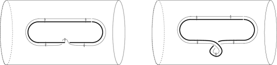
Figure 1: The rotation or exchange loop

It is possible to describe a framing without drawing any normal vectors at all. The first vector may be taken perpendicular to the plane of the figure, the second vector may be obtained from the cross product with the tangent vector, and the third vector may be taken to be the suppressed $z$-direction. The framing obtained by following this convention is called the black board framing. We use the blackboard framing in figure 2. The Pontrjagin-Thom construction may also be used to visualize loops in other components of the configuration space. Figure 2 shows a loop in the degree $2$ component of the space of maps from $M$ to Sp$(1)$.

Figure 2: The degree $2$ exchange loop

We can also use the Pontrjagin-Thom construction to draw figures of homotopies between loops in configuration space. Figure 3 displays a homotopy between the loop corresponding to a canonically framed unknot and the constant loop. In this figure, the horizontal direction represents the second interval factor of $M\times[0,1]\times[0,1]$, the direction out of the page represents the first interval factor, the vertical direction represents the $x$ direction, and the $y$ and $z$ directions are suppressed. The framing is given by the normal vector to the hemisphere, the $y$ direction and the $z$ direction.

Figure 3: The contraction of a canonically framed contractible link

4.3 Cohomology of $G^{M}$

We now turn to a description of the real cohomology of $G^{M}$. We will use the slant product to associate a cohomology class on $G^{M}$ to a pair consisiting of a homology class on $M$ and a cohomology class on $G$. Recall that the slant product is a map $H^{n}(X\times Y;A)\otimes H_{k}(X;B)\to H^{n-k}(Y;A\otimes B)$, [33]. In addition the universal coefficient theorem allows us to identify $H^{k}(G^{M};{\mathbb{R}})$ with $\hbox{Hom}(H_{k}(G^{M};{\mathbb{Z}}),{\mathbb{R}})$. Let $\sigma:\Sigma\to M$ be a singular chain representing a homology class in $H_{d}(M;{\mathbb{R}})=H_{d}(M;{\mathbb{Z}})\otimes{\mathbb{R}}$ (instead of viewing singular chains as linear combinations of singular simplicies, we will combine them together and view a singular chain as a map of a special polytope into the space), and let $x_{j}$ be a cohomology class in $H^{j}(G;{\mathbb{R}})$. To define the image of the mu map, $\mu(\Sigma\otimes x_{j})$, let $u:F\to G^{M}$ be a singular chain representing an element in the $H_{d-j}(G^{M})$. This induces a natural singular chain $\widehat{u}:M\times F\to G$. The pull back produces $\widehat{u}^{*}x_{j}\in H^{j}(M\times F;{\mathbb{R}})$. The formal definition of the mu map is then,

$$\mu(\Sigma\otimes x_{j})(u):=(\widehat{u}^{*}x_{j}/\Sigma)[F].$$ (4.1)

Writing this in notation from the de Rham model of cohomology may help to clarify the definitions. In principle one could construct a homology theory based on smooth chains and make the following rigorous. The $\mu$ map produces a $(j-d)$-cocycle in $G^{M}$ from a $d$-cycle in $M$ and a $j$-cocycle in $G$. On the level of chains, let $e^{d}:D^{d}\to M$ be a $d$-cell, and $x_{j}$ be a closed $j$-form on $G$. Given a singular simplex, $u:\Delta^{j-d}\to G^{M}$, let $\widehat{u}:M\times\Delta^{j-d}\to G$ be the natural map and write

$$\mu(e^{d}\otimes x_{j})(u)=\int_{D^{d}\times\Delta^{j-d}}\widehat{u}^{*}x_{j}.$$

Using the product formula for the boundary,

$$\partial(D^{d}\times\Delta^{j-d+1})=(\partial D^{d})\times\Delta^{j-d+1}+(-1)^{d}D^{d}\times\partial\Delta^{j-d+1},$$

we can get a simple formula for the coboundary of the image of an element under the $\mu$-map. Let $v:\Delta^{j-d+1}\to G^{M}$, be a singular simplex, then

$$\delta(\mu(e^{d}\otimes x_{j}))(v) = \sum_{k=0}^{j-d+1}(-1)^{k}\int_{D^{d}\times\Delta^{j-d}}\widehat{(v\circ f_{k})}^{*}x_{j}=\int_{D^{d}\times\partial\Delta^{j-d+1}}\widehat{v}^{*}x_{j}$$ (4.2)

$$= (-1)^{d+1}\int_{(\partial D^{d})\times\Delta^{j-d+1}}\widehat{v}^{*}x_{j}+(-1)^{d}\int_{\partial(D^{d}\times\Delta^{j-d+1})}\widehat{v}^{*}x_{j}$$

$$= (-1)^{d+1}\mu((\partial e^{d})\otimes x_{j})(v).$$

We used Stokes’ theorem in the last line. It follows that $\mu$ is well defined at the level of homology. Theorem 3 asserts that $H^{*}(G^{M}_{0};{\mathbb{R}})$ is a finitely generated algebra with generators $\mu(\Sigma_{j}^{d}\otimes x_{k})$ where $\{\Sigma_{j}^{d}\}$ and $\{x_{k}\}$ are bases for $H_{*}(M;{\mathbb{R}})$ and $H^{*}(G;{\mathbb{R}})$ respectively. The multiplication on $H^{*}(G^{M};{\mathbb{R}})$ is given by the cup product. Recall that this is defined at the level of cochains by, $(\alpha\smallsmile\beta)(w)=\alpha(~{}_{k}w)\beta(w_{\ell})$, where $\alpha$ is a $k$-cocycle, $\beta$ is a $\ell$-cocycle, $w$ is a $(k+\ell)$-singular simplex and $~{}_{k}w$ is the front $k$-face and $w_{\ell}$ is the back $\ell$-face [33]. Note that $\smallsmile$ is graded-commutative, that is, $\alpha\smallsmile\beta=(-1)^{k\ell}\beta\smallsmile\alpha$.

It is instructive to understand some classes that do not appear as generators. One might expect $\mu(\hbox{pt}\otimes x_{j})$ to be a generator in degree $j$. However, since $G^{M}$ consists of based maps, the induced map $\widehat{u}:M\times F\to G$ arising from a chain $u:F\to G^{M}$ restricts to a constant map on $\hbox{pt}\times F$. It follows that $\mu(\hbox{pt}\otimes x_{j})=0$. There would be an analogous class if we considered the cohomology of the space of free maps. Turning to the other end of the spectrum, one might expect to see classes of the form $\mu(M\otimes x_{3})$ in degree zero. Such certainly could not appear in the cohomology of the identity component $G^{M}_{0}$. In fact we stated our theorem for the identity component because the argument leading to generators of the form $\mu(\Sigma\otimes x_{3})$ breaks down when $\Sigma$ is a $3$-cycle and $x_{3}$ is a $3$-cocycle. The argument starts by considering maps of spheres into the group $G$, and then assembles the cohomology of these mapping spaces (which are denoted by $\Omega^{k}G$) into the cohomology of $G^{M}$. The path fibration is used to compute the cohomology of the $\Omega^{k}G$. The fibration leading to the cohomology of $\Omega^{3}G$ does not have a simply connected base and this is the break down. See Lemma 15. Finally one might expect to see classes of the form $\mu(\Sigma\otimes x_{j}\cup x_{k})$. It will turn out in the course of the proof (Lemma 15) that such classes vanish.

Up to this point, our geometric descriptions of the algebraic topology of configuration spaces have been simpler than we had any right to expect. We were able to describe the space of path components and the fundamental group of the configuration space of maps from an orientable $3$-manifold into an arbitrary simply-connected Lie group by just considering subgroups isomorphic to Sp$(1)$. This will not hold for all homotopy invariants of $G^{M}$. The main object of interest to us is the second cohomology of the configuration space with integral coefficients, because this classifies the complex line bundles over the configuration space (the quantization ambiguitity). It is possible to describe one second cohomology class on Sp$(n)^{M}$ in terms of Sp$(1)$ geometry. However we need to pass to SU$(3)$ subgroups to get at the second cohomology in general.

Before considering these geometric representatives of the second cohomology, briefly recall the definition of the Ext groups. Given $R$-modules $A$ and $B$ pick a free resolution of $A$ say $\to C_{2}\to C_{1}\to C_{0}\to A$. The $k$th Ext group is just defined to be the $k$th homology of the complex $\hbox{Hom}(C_{*},B)$, i.e. $\hbox{Ext}^{k}_{R}(A,B)=H_{k}(\hbox{Hom}(C_{*},B))$. When $R$ is a PID (principal ideal domain) every $R$-module has a free resolution of the form, $0\to C_{1}\to C_{0}\to A$. Given such a resolution one obtains the exact sequence,

$$0\to\hbox{Hom}(A,B)\to\hbox{Hom}(C_{0},B)\to\hbox{Hom}(C_{1},B)\to\hbox{Ext}^{1}_{R}(A,B)\to 0,$$ (4.3)

and all higher Ext groups vanish. We will always take $R={\mathbb{Z}}$ and drop the ground ring from the notation. Based on the above exact sequence, we say that the Ext groups measure the failure of Hom to be exact i.e. take exact sequences to exact sequences. The Ext group may also be identified with the collection of extensions of $A$ by $B$ [33]. By the universal coefficient theorem

$$\begin{array}[]{rcl}H^{2}(G^{M};{\mathbb{Z}})&\cong&\hbox{Ext}^{1}(H_{1}(G^{M};{\mathbb{Z}}),{\mathbb{Z}})\oplus\hbox{Hom}(H_{2}(G^{M};{\mathbb{Z}}),{\mathbb{Z}})\\ H^{2}(G^{M};{\mathbb{R}})&\cong&\hbox{Ext}^{1}(H_{1}(G^{M};{\mathbb{Z}}),{\mathbb{R}})\oplus\hbox{Hom}(H_{2}(G^{M};{\mathbb{Z}}),{\mathbb{R}})\end{array}$$

Now for all $A$, $\hbox{Ext}^{1}(A,{\mathbb{R}})=0$, so $\hbox{Hom}(H_{2}(G^{M};{\mathbb{Z}}),{\mathbb{Z}})$ is a free abelian group of rank $b_{2}=\hbox{dim}_{{\mathbb{R}}}H^{2}(G^{M};{\mathbb{R}})$. In addition, $\hbox{Ext}^{1}(A,{\mathbb{Z}})$ is just the torsion subgroup of $A$ and $H_{1}(G^{M};{\mathbb{Z}})\cong\pi_{1}^{\rm ab}(G^{M})=\pi_{1}(G^{M})$. Hence

$$H^{2}(G^{M};{\mathbb{Z}})\cong{\mathbb{Z}}^{b_{2}}\oplus{\rm Tor}(\pi_{1}(G^{M}))$$

where $\pi_{1}(G^{M})$ and the Betti number $b_{2}$ may be obtained from Theorems 2 and 3.

We will use the universal coefficient theorem and Ext groups to describe some cohomology classes of our configuration spaces. There is a natural ${\mathbb{Z}}_{2}$ contained in the fundamental group of the configuration space for any group with a symplectic factor. This ${\mathbb{Z}}_{2}$ is generated by the exchange loop. Wrapping twice around the exchange loop is the boundary of a disk in the configuration space. Since ${\mathbb{R}}P^{2}$ is the result of identifying the points on the boundary of a disk via a degree $2$ map, one expects to find an ${\mathbb{R}}P^{2}$ embedded into any of the Skyrme configuration spaces with a symplectic factor. In [32], R. Sorkin describes an embedding, $f_{\rm{stat}}:{\mathbb{R}}P^{2}\to\hbox{SU}(n+1)^{S^{3}}$. He also describes an embedding, $f_{\rm{spin}}:{\mathbb{R}}P^{3}\to\hbox{SU}(n+1)^{S^{3}}$. He further shows that $f_{\rm{spin}}$ restricted to the ${\mathbb{R}}P^{2}$ subspace is homotopic to $f_{\rm{stat}}$. Using the map, $M\to M^{(3)}/M^{(2)}\cong S^{3}$, these induce maps into SU$(n+1)^{M}$. Here $M^{(k)}$ is the $k$ skeleton of $M$ with respect to some CW structure. In fact, using the inclusion of Sp$(1)=\hbox{SU}(2)$ into any simply-connected simple Lie group one obtains maps from ${\mathbb{R}{{P}}}^{2}$ and ${\mathbb{R}{{P}}}^{3}$ into any configuration space of Lie group valued maps. This is most interesting when the map factors through a symplectic factor.

We briefly recall Sorkin’s elegant construction. Describe ${\mathbb{R}}P^{2}$ as the $2$-sphere with antipodal points identified. By the addition of particle antiparticle pairs, we may assume that there are two particles in a coordinate chart. We may place the particles at antipodal points of a sphere in a coordinate chart using frames parallel to the coordinate directions. The map obtained from these frames using the Pontrjagin-Thom construction is $f_{\rm{stat}}$. The projective space, ${\mathbb{R}}P^{3}$ is homeomorphic to the rotation group SO$(3)$. The map $f_{\rm{spin}}$ may be described by using SO$(3)$ to rotate a single frame and then applying the Pontrjagin-Thom construction. Sorkin includes a second unaffected particle in his description of $f_{\rm{spin}}$ to make the comparison with $f_{\rm{stat}}$ easier.

A degree one map $M\to S^{3}$ (which always exists) induces a map $G^{S^{3}}\to G^{M}$. The space $G^{S^{3}}$ is typically denoted $\Omega^{3}G$. If the Lie algebra of the maximal compact subgroup admits a symplectic factor, then we have an interesting map Sp$(1)\to G$ which induces a map $\Omega^{3}\hbox{Sp}(1)\to\Omega^{3}G$. We will see in the course of our proofs that on the level of $\pi_{1}$ or $H_{1}$ these maps give a sequence of injections,

$$H_{1}({\mathbb{R}{{P}}}^{2};{\mathbb{Z}})\to H_{1}({\mathbb{R}{{P}}}^{3};{\mathbb{Z}})\to H_{1}(\Omega^{3}\hbox{Sp}(1);{\mathbb{Z}})\to H_{1}(\Omega^{3}G;{\mathbb{Z}})\to H_{1}(G^{M};{\mathbb{Z}}).$$

The universal coefficient theorem implies that there is a ${\mathbb{Z}}_{2}$ factor in the second cohomology of $G^{M}$ when $G$ contains a symplectic factor. In fact, in this case we see that twice the exchange loop is a generator of the $1$-dimensional boundaries. This means we can define a homomorphism from $B_{1}$ (the $1$-dimensional boundaries) to ${\mathbb{Z}}$ taking twice the exchange loop to $1$. The cocycle defined by following the boundary map from $2$-chains by this homomorphism generates the ${\mathbb{Z}}_{2}$ in $H^{2}(G^{M};{\mathbb{Z}})$. We see that this class evaluates nontrivially on the Sorkin ${\mathbb{R}{{P}}}^{2}$.

When $G$ has unitary factors, there will be infinite cyclic factors in the second cohomology of $G^{M}$. This is nicely explained by a construction of Ramadas, [28]. Ramadas constructs a map, $S^{2}\times S^{3}\to\hbox{SU}(3)$. This construction goes as follows. He first defines a map $K:\hbox{SU}(2)\to\hbox{SU}(2)$ by

$$K(\left(\begin{array}[]{cc}a&b\\ -\bar{b}&\bar{a}\end{array}\right))=(|a|^{4}+|b|^{4})^{-\frac{1}{2}}\left(\begin{array}[]{cc}a^{2}&-\bar{b}^{2}\\ b^{2}&\bar{a}^{2}\end{array}\right).$$

This map satisfies, $K(\hbox{diag}(\lambda,\bar{\lambda})A)=K(A)\hbox{diag}(\lambda^{2},\bar{\lambda}^{2})$. Finally define $\widehat{\sigma}:S^{1}\backslash\hbox{SU}(2)\times\hbox{SU}(2)\to\hbox{SU}(3)$ by

$$\widehat{\sigma}([A],B)=\hbox{diag}(1,K(A))\hbox{diag}(ABA^{*},1)\hbox{diag}(1,K(A)^{*}).$$

Here we are viewing $S^{1}$ as the subgroup $\hbox{diag}(\lambda,\bar{\lambda})$ of SU$(2)$. It is well known that $S^{1}\backslash\hbox{SU}(2)\cong S^{2}$ and SU$(2)\cong S^{3}$. The map $\widehat{\sigma}:S^{2}\times S^{3}\to\hbox{SU}(3)$ induces a map $\sigma:S^{2}\to\Omega^{3}\hbox{SU}(3)$. Ramadas shows that this map generates $H_{2}(\Omega^{3}\hbox{SU}(3);{\mathbb{Z}})\cong{\mathbb{Z}}$. Combining with the degree one map from $M$ and the inclusion into a special unitary factor of $G$, we obtain a map $S^{2}\to G^{M}$ generating an infinite cyclic factor of $H_{2}(G^{M};{\mathbb{Z}})$. By the universal coefficient theorem a map from $H_{2}(G^{M};{\mathbb{Z}})$ to ${\mathbb{Z}}$ taking this generator to $1$ is a cohomology class in $H^{2}(G^{M};{\mathbb{Z}})$. Clearly this class evaluates non-trivially on this $S^{2}$.

If $G$ does not have a symplectic or special unitary factor, then there is no reason to expect any elements of the second cohomology. In fact under this hypothesis, $H^{2}(\Omega^{3}G;{\mathbb{Z}})=0$. It is worth mentioning how these maps behave in general. The third homotopy group of any Lie group is generated by homomorphic images of Sp$(1)$. Each time one of these generators is contained in a symplectic factor, we get a ${\mathbb{Z}}_{2}$ in the second cohomology detected by a Sorkin ${\mathbb{R}{{P}}}^{2}$. When one of these factors is not contained in a symplectic factor, it is contained in a copy of SU$(3)$. This kills the ${\mathbb{Z}}_{2}$ factor in $\pi_{1}$ as explained above in subsection 4.2. If the SU$(3)$ is contained in a special unitary factor, the Sorkin map ${\mathbb{R}{{P}}}^{2}\to\hbox{Sp}(1)^{M}\to\hbox{SU}(3)^{M}\to G^{M}$ pulls back the second cohomology class described by Ramadas (and extended to arbitrary $M$ and $G$ with special unitary factor as above) to the generator of $H^{2}({\mathbb{R}{{P}}}^{2};{\mathbb{Z}})\cong{\mathbb{Z}}_{2}$. (Ramadas proves that the generator of $H^{2}(\Omega^{3}\hbox{SU}(3);{\mathbb{Z}})$ pulls back to the generator of $H^{2}({\mathbb{R}{{P}}}^{2};{\mathbb{Z}})$ and the rest follows from our proofs.) If this SU$(3)$ is not contained in a special unitary factor, it follows from our proofs that the second homology class associated to $S^{2}\to G^{M}$ bounds, so there is no associated cohomology class.

4.4 Components of $(S^{2})^{M}_{\varphi}$

The picture of the components of $(S^{2})^{M}_{\varphi}$ arising from the Pontrjagin-Thom construction and Poincaré duality is quite nice. The inverse image of a regular point in $S^{2}$ is Poincaré dual to $\varphi^{*}\mu_{S^{2}}$. The number of twists in the framing of a second map with the same pull-back is the element of $H^{3}(M;{\mathbb{Z}})/\langle 2\varphi^{*}\mu_{S^{2}}\rangle$. This is very similar to the description of elements of the fundamental group of $G^{M}$ when $G$ has symplectic factors. We will identify $S^{2}$ with ${\mathbb{C}}{\mathbb{P}}^{1}$ and consider several maps. We have $\varphi_{1},\varphi_{1}^{\prime},\varphi_{3}:{\mathbb{C}}{\mathbb{P}}^{1}\times S^{1}\to{\mathbb{C}}{\mathbb{P}}^{1}$ given by,

$$\varphi_{1}([z:w],\lambda)=[z:w],\qquad\varphi_{1}^{\prime}([z:w],\lambda)=[\lambda z:w],\quad\hbox{and}\quad\varphi_{3}([z:w],\lambda)=[z^{3}:w^{3}].$$

We can view ${\mathbb{C}}{\mathbb{P}}^{1}\times S^{1}$ as $S^{2}\times[0,1]$ (a spherical shell) with the inner and outer ($S^{2}\times\{0\}$ and $S^{2}\times\{0\}$) spheres identified. Using this convention and the framing conventions from subsection 4.2, We have displayed the framed $1$-manifolds arising as the inverse image of a regular point in figure 4.

Figure 4: Pontrjagin-Thom representatives of $S^{2}$-valued maps

It may appear that there is a well defined twist number associated to a $S^{2}$-valued map. However, there is a homeomorphism of ${\mathbb{C}}{\mathbb{P}}^{1}\times S^{1}$ twisting the $2$-sphere (such a map is given by $([z:w],\lambda)\mapsto([\lambda z:w],\lambda)$). This will change the number of twists in a framing, but will not change the relative number of twists. The reason why this relative number of twists is only well defined modulo twice the divisibility of the cohomology class $\varphi^{*}\mu_{S^{2}}$ is demonstrated for $\varphi_{1}$ in figure 5.

Figure 5: Introducing $2d$ twists

4.5 Fundamental group of $(S^{2})^{M}_{\varphi}$

An element of $\pi_{1}((S^{2})^{M}_{\varphi})$ is represented by a map, $\gamma:M\times S^{1}\to S^{2}$. The inverse image of a regular point is a $2$-dimensional submanifold, say $\Sigma$. This defines an element of $H^{1}(M;{\mathbb{Z}})$ as follows. To any $1$-cycle in $M$, say $\sigma$, we associate the intersection number of $\Sigma$ and $\sigma\times S^{1}$. Since our loop is in the path component of $\varphi$, the surface $\Sigma$ is parallel to the $\varphi$-inverse image of a regular point. This implies that our element of $H^{1}(M;{\mathbb{Z}})$ is in the kernel of the map, $2\varphi^{*}\mu_{S^{2}}:H^{1}(M;{\mathbb{Z}})\to H^{3}(M;{\mathbb{Z}})$. Given any element of this kernel, we can define a loop in $(S^{2})^{M}_{\varphi}$ via the ${\mathfrak{q}}$-map defined below at line 6.2. There is a map from $u:M\times S^{1}\to\hbox{Sp}(1)$ that may be used to change this new loop back into $\gamma$. The remaining homotopy invariants of $\gamma$ are just those of $u$ as described in subsection 4.2.

5 Physical consequences

As explained in section 3, the configuration space of the Skyrme model with arbitrary target group is homotopy equivalent to the configuration space of a collection of uncoupled Skyrme fields each taking values in a compact, simply connected, simple Lie group. We will therefore assume, throughout this section that $G$ is compact, simply connected and simple. In this case, by Proposition 1, the path components of $G^{M}$ are labeled by $H^{3}(M;{\mathbb{Z}})\cong{\mathbb{Z}}$, identified with the baryon number $B$ of the configuration. This identification has already been justified by consideration of the Pontrjagin-Thom construction. Let us denote the baryon number $B$ sector by $Q_{B}$.

We first recall how Finkelstein and Rubinstein introduced fermionicity to the Skyrme model [15]. The idea is that the quantum state is specified by a wavefunction on $\widetilde{Q}_{B}$, the universal cover of $Q_{B}$, rather than $Q_{B}$ itself. By the uniqueness of lifts, there is a natural action of $\pi_{1}(Q_{B})$ on $\widetilde{Q}_{B}$ by deck transformations. Let $\pi:\widetilde{Q}_{B}\rightarrow Q_{B}$ denote the covering projection, $\lambda\in\pi_{1}(Q_{B})$ and $D_{\lambda}$ be the associated deck transformation. Since all points in $\pi^{-1}(u)$ are physically indistinguishable, we must impose the constraint

$$|\psi(D_{\lambda}q)|=|\psi(q)|$$

on the wavefunction $\psi:\widetilde{Q}_{B}\rightarrow{\mathbb{C}}$, for all $q\in\widetilde{Q}_{B}$ and $\lambda\in\pi_{1}(Q_{B})$. This leaves us the freedom to assign phases to the deck transformations, that is, the remaining quantization ambiguity consists of a choice of $U(1)$ representation of $\pi_{1}(Q_{B})$. The possibility of fermionic quantization arises if the two-Skyrmion exchange loop in $Q_{2}$ is noncontractible with even order: we can then choose a representation which assigns this loop the phase $-1$. In this case our wavefunction aquires a minus sign under Skyrmion interchange. Clearly, the Finkelstein-Rubinstein model could apply to any sigma model with a configuration space admiting non-trivial elements of the fundamental group representing the exchange of identical particles. In particular, the domain does not have to be ${\mathbb{R}}^{3}$.

Note we have insisted that the wavefunction $\psi$ have support on a single path component $Q_{B}$, because baryon number is conserved in nature, so transitions which change $B$ have zero probability. It seems, then, that the choice of representation of $\pi_{1}(Q_{B})$ can be made independently for each $B$, but in fact there is a strong consistency requirement between the representations associated with the various components. Recall that all the sectors are homeomorphic and that given any $u\in Q_{B}$ one obtains a homeomorphism $Q_{0}\rightarrow Q_{B}$ by pointwise multiplication by $u$. Hence, to each $u\in Q_{B}$ there is associated an isomorphism $\pi_{1}(Q_{0})\rightarrow\pi_{1}(Q_{B})$, so one has a map $Q_{B}\rightarrow{\rm Iso}(\pi_{1}(Q_{0}),\pi_{1}(Q_{B}))$. Since $Q_{B}$ is connected and $\pi_{1}$ is discrete, this map is constant, that is, there is a canonical isomorphism $\pi_{1}(Q_{0})\rightarrow\pi_{1}(Q_{B})$, which may be obtained by pointwise multiplication by any charge $B$ configuration. Having chosen a representation of $\pi_{1}(Q_{0})$, we obtain canonical representations of $\pi_{1}(Q_{B})$ for all other $B$. Physically, we are demanding that the phase introduced by transporting a configuration around a closed loop should be independent of the presence of static Skyrmions held remote from the loop. This places nontrivial consistency conditions, if we are to obtain a genuinely fermionic quantization. In particular, the loop in $Q_{2B}$ consisting of the exchange of a pair of identical charge $B$ Skyrmions must be assigned the phase $(-1)^{B}$, since a charge $B$ Skyrmion represents a bound state of $B$ nucleons, which is a fermion for $B$ odd and a boson for $B$ even.

The Finkelstein-Rubinstein formalism can be used to give a consistent fermionic quantization of the Skyrme model on any domain $M$ if $G={\rm Sp}(n)$, but not for any of the other simple target groups. In this case, Theorem 2 tells us that

$$\pi_{1}(Q_{B})\equiv{\mathbb{Z}}_{2}\oplus H_{1}(M)$$

and we can choose (and fix) a $U(1)$ representation which maps the generator of ${\mathbb{Z}}_{2}$ to $(-1)$. The generator of the ${\mathbb{Z}}_{2}$-factor in the baryon number zero component is exactly the rotation–exchange loop as may be seen in the proof of proposition 13 in the next section. To see that this assigns phase $(-1)$ to the 2-Skyrmion exchange loop, we may consider the Pontrjagin-Thom representative of the loop. This is a framed 1-cycle in $S^{1}\times M$ depicted in figure 6. It is framed-cobordant to the representative of the loop in which one of the Skyrmions remains static, while the other rotates through $2\pi$ about its center. Figure 6 gives a sketch of the cobordism. The horizontal direction represents the loop parameter (“time”), the vertical direction represents $M$ and the direction into the page represents the cobordism parameter. The framing has been omitted, and the start and end 1-cycles of the cobordism have been repeated, for clarity. Note that the apparent self intersection of the cobordism (along the dashed line) is an artifact of the pictorial projection from 5 dimensions to 3. Hence, the exchange loop in $Q_{2}$ is homotopic to the loop represented by one static Skyrmion and one Skyrmion that undergoes a full rotation.

To identify the phase assigned to this homotopy class, we must transfer the loops to $Q_{0}$ by adding a pair of anti-Skyrmions, as depicted in figure 7. This changes each configuration by multiplying by a fixed charge $-2$ configuration which is $1$ outside a small ball – precisely one of the homeomorphisms discussed above. The figure may be described thus: the exchange loop is homotopic to the rotation loop with an extra static $1$-Skyrmion lump (far left) which is transferred to the vacuum sector by adding a stationary pair of anti-Skyrmions (2nd box). This loop is homotopic to the charge $0$ rotation loop of figure 1, via the sequence of moves shown. The orientations on the curves indicate how to assign a framing via the blackboard framing convention. The resulting Pontrjagin-Thom representative is framed cobordant to the charge $0$ exchange loop described in section 4.2, which, as explained, generates the ${\mathbb{Z}}_{2}$ factor in $\pi_{1}(Q_{0})$. Hence, the loop along which two identical $1$-Skyrmions are exchanged (without rotating) around a contractible path in $M$ is assigned the phase $(-1)$.

Figure 6: The cobordism between Skyrmion rotation and Skyrmion exchange.

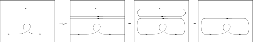
Figure 7: Mapping the Skyrmion exchange loop into the vacuum sector $Q_{0}$.

Figure 8: Exchange of baryon number 2 Skyrmions is contractible in $Q_{4}$.

Exchange of higher charge Skyrmions may be treated by considering composites of $B$ unit Skyrmions, as depicted for $B=2$ in figure 8. The loop may be deformed into one with four distinct single exchange events (surrounded by dashed boxes). Each of these may be replaced by a pair of uncrossed strands, one of which has a $2\pi$ twist, using the homotopy described in figures 1 and 6 in each box. Since each strand has an even number of twists, this is homotopic to the constant loop. Hence it must be assigned the phase $(+1)$. The argument clearly generalizes: given an exchange loop of a pair of charge $B$ composites, one may isolate $B^{2}$ single exchange events, each of which can be replaced by a single twist in one of the uncrossed strands. It is easy to see that the twists may be distributed so that every strand except at most one has an even number of twists. Hence if $B$ is even, this last strand also has an even number of twists and the loop is necessarily contractible. If $B$ is odd, the last strand has an odd number of twists, so the loop is homotopic to the loop where $2B-1$ Skyrmions remain static and one Skyrmion executes a $2\pi$ twist. Adding $2B$ anti-Skyrmions, this loop is identified with the baryon number $0$ exchange loop and hence receives a phase of $(-1)$.

Finkelstein and Rubinstein also model spin in this framework. In this model spin is determined by the phase associated to the rotation loop. As we saw in the previous section the rotation and exchange loops agree up to homotopy confirming the spin statistics theorem in this model. This is essentially the observation that the exchange loop is homotopic to the $2\pi$ rotation loop (figure 6).

Note that throughout the above discussion we have used only a local version of exchange to model particle statistics, and verify the spin-statistics correlation. This definition of particle statistics and spin makes sense on general $M$, even without an action of $SO(3)$, because the exchange and rotation loops have support over a single coordinate chart, so we have a local notion of rotating a Skyrmion. Things become much more subtle when a loop has Pontrjagin-Thom representative which projects to a nontrivial cycle in $M$. It should not be surprising that it requires a spin structure on $M$ to specify whether the constituent Skyrmions of such a loop undergo an even or odd number of rotations. It was precisely the generalization from ${\mathbb{R}}^{3}$ to general spaces that motivated the definition of spin structures in the first place. Notice that by changing the spin structure, we can interpret a loop as either having an even or odd number of rotations, so one must fix a spin structure on space before discussing spin. (This is similar to the reason, discussed in section 4.4 above, why the secondary invariant for path components of $S^{2}$-valued maps is only a relative invariant). Even in the simple case of quantization of many point particles on a topologically nontrivial domain, the statistical type (boson, fermion or something more exotic) of the particles is usually taken to be determined only by their exchange behavior around trivial loops in $M$ [21]. It may be more reasonable to require that spin be determined by the behavior of locally supported rotations, but to insist that the statistical type be consistent under any particle exchange. It follows from Proposition 13 that the notion of an exchange or rotation loop around a contractible loop is well defined independent of the choice of spin structure. This is just the image of $\pi_{4}(G)$. That the parity of a rotation around a non-contractible loop is determined by a spin structure is explained in Proposition 14 in the next section.

In fact, the Finkelstein-Rubinstein quantization scheme remains consistently fermionic in this extended sense provided that the correct representation into U$(1)$ is chosen. As with more traditional models of spin, a spin structure on the domain will be required. When the domain has non trivial first cohomology with ${\mathbb{Z}}_{2}$ coefficients there are many spin structures to choose from. Selecting a spin structure produces an isomorphism of $\pi_{1}(Q_{B})$ with ${\mathbb{Z}}_{2}\oplus H_{1}(M)$. The required representation is just projection onto the ${\mathbb{Z}}_{2}$ factor. Exchange around a (possibly) non-contractible simple closed curve in space means that two identical solitons start at antipodal points on the curve and each one moves without rotating half way around the curve to exchange places with the other soliton. The notion of moving without rotating is where the spin structure enters. We will define this after describing the representation of an exchange displayed in figure 9. Each rectangle in this figure represents a slice of a cobordism. The horizontal direction represents time, the vertical direction represents space, and the thick lines are the world lines of the solitons. The top and bottom of each rectangle are to be identified to make each slice a cylinder representing the curve cross time. We can imagine different spin structures obtained by identifying the top and bottom in the straight-forward way or by putting a full twist before making the identification. The first slice is just the exchange around the curve. One of the loops makes a left hand rotation followed by a right hand rotation, but this wobble is the same as no rotation at all. Adding a ribbon between the non-rotating soliton and the right rotation of the bottom soliton produces the second slice. This slice may be described as one soliton making a full left rotation in a fixed location while a second soliton traverses once around the curve without rotation. This slice homotopes to the third slice, and a second ribbon gives the fourth slice. The fourth slice may be described as follows. The vertical S-curve represents the birth of a Skyrmion anti-Skyrmion pair after which the Skyrmion and anti-Skyrmion move in opposite directions around the curve until they collide and annihilate. The horizontal lines are two (nearly) static Skyrmions, and the figure eight curve is a contractible (left) rotation loop. By definition, the exchange is non-rotating with respect to the spin structure if the ${\mathbb{Z}}_{2}$ representation of the vertical S-curve resulting from a baryon number $1$ exchange is trivial. We now see that the general exchange is consistent because the two horizontal lines contribute nothing to the representation, the S-curve contributes nothing, and the baryon number $B$ contractible rotation loop contributes $(-1)^{B}$ as described previously and seen in figure 8.

Figure 9: Sum of a loop with the rotation loop.

As will be seen in section 6.3, there is a close connexion between ${\rm Sp}(1)^{M}$ and $(S^{2})^{M}$. This allows us to transfer the Finkelstein-Rubinstein construction of a fermionic quantization scheme for ${\rm Sp}(N)$ valued Skyrmions to the Faddeev-Hopf model. Recall that here, unless $H^{2}(M;{\mathbb{Z}})=0$, the path components of $Q$ are not labelled simply by an integer, but rather are separated by an invariant $\alpha\in H^{2}(M)$, and a relative invariant $c\in H^{3}(M)/2\alpha\smallsmile H^{1}(M)$. Configurations with $\alpha\neq 0$ necessarily have support which wraps around a nontrivial cycle in $M$. They therefore lack one of the key point-like characteristics of conventional solitons: they are not homotopic to arbitrarily highly localized configurations. Such configurations are intrinsically tied to some topological “defect” in physical space, and so are somewhat exotic. We therefore, mainly restrict our attention to configurations with $\alpha=0$. As with Skyrmions, these configurations are labelled by $B\in{\mathbb{Z}}\cong H^{3}(M;{\mathbb{Z}})$ which we identify with the Hopfion number. This is the relative invariant between the given configuration and the constant map. It turns out that all the $\alpha=0$ sectors, $Q_{B}$, are homeomorphic (Theorem 5) and, further, that $Q_{B}$ is homotopy equivalent to $({\rm Sp}(1))^{M}_{0}$, the vacuum sector of the classical Skyrme model. The homotopy equivalence is given by the fibration $f^{*}$ of Lemma 20. This may be used to map the charge zero Skyrmion exchange loop to a charge 2 Hopfion exchange loop, generating a ${\mathbb{Z}}_{2}$ factor in $\pi_{1}(Q_{2})$. It follows that Hopfions can be quantized fermionically within the Finkelstein-Rubinstein scheme. In the more exotic configurations with $\alpha\neq 0$, the relative invariant takes values in ${\mathbb{Z}}/(2d{\mathbb{Z}})\cong H^{3}(M;{\mathbb{Z}})/(2\alpha\smile H^{1}(M;{\mathbb{Z}}))$. So even though the Hopfion number is not defined in this case, the parity of the Hopfion number is well defined and the Finkelstein-Rubinstein formalism still yields a consistently fermionic quantization scheme.

We return now to the Skyrme model, but in the case where $G$ is not ${\rm Sp}(N)$ but is rather ${\rm SU}(N)$, ${\rm Spin}$ or exceptional. In this case the Skyrmion exchange loop is contractible, so must be assigned phase $(+1)$ in the Finkelstein-Rubinstein quantization scheme so that only bosonic quantization is possible in that framework. To proceed, one may take the wavefunction to be a section of a complex line bundle over $Q_{B}$ equipped with a unitary connexion. Parallel transport with respect to the connexion associates phases to closed loops in $Q_{B}$ in a way that one might hope will mimic fermionic behaviour. The problem with this is that the holonomy of a loop is not (for non-flat connexions) homotopy invariant, so the phase assigned to an exchange loop will depend on the fine detail of how the exchange is transacted. To get round this, Sorkin introduced a purely topological definition of statistical type and spin for solitons defined on ${\mathbb{R}}^{3}$. His definition extends immediately to solitons defined on arbitrary domains. We review these definitions next.

Recall Sorkin’s definition of $f_{\rm stat}:{\mathbb{R}{{P}}}^{2}\rightarrow Q_{2}$: choose a sphere in ${\mathbb{R}}^{3}$ and associate to each antipodal pair of points on this sphere the charge 2 configuration with Pontrjagin-Thom representation given by that pair of points, framed by the coordinate basis vectors. The subscript stat in $f_{\rm stat}$ refers to statistics. There is an associated homomorphism $f_{\rm stat}^{*}:H^{2}(Q_{2})\rightarrow H^{2}({\mathbb{R}{{P}}}^{2})\cong{\mathbb{Z}}_{2}$ given by pullback. According to Sorkin’s definition, the quantization wherein the wavefunction is a section of the line bundle over $Q$ associated with class $c\in H^{2}(Q;{\mathbb{Z}})$ is fermionic if $f_{\rm stat}^{*}(c)=1$, bosonic otherwise, [32]. Thinking of $f_{\rm stat}$ as an inclusion map, the pulled-back class $f_{\rm stat}^{*}(c)$ represents the Chern class of the restriction of the bundle associated to $c$ over $Q_{2}$ to the subset ${\mathbb{R}{{P}}}^{2}$. The intuition behind this definition is that if there was a unitary connection on the bundle with parallel transport equal to $(-1)$ around exchange loops, then the restriction to the bundle to such a ${\mathbb{R}{{P}}}^{2}$ would have to be non-trivial. This definition generalizes to solitons defined on arbitrary domains by analogous maps from ${\mathbb{R}{{P}}}^{2}$ into the configuration space based on embeddings of $S^{2}$ in the domain. To make sense of the framing, one must pick a trivialization of the tangent bundle of the domain restricted to the $S^{2}$. Up to homotopy there is a unique such framing. The elementary Sorkin maps will be the ones associated with sufficiently small spheres that lie in a single coordinate chart.

To model spin for solitons with domain ${\mathbb{R}}^{3}$, Sorkin considers the action of SO$(3)$ on the configuration space given by precomposition with any field. The orbit of a basic soliton with Pontrjagin-Thom representative given by one point and an arbitrary frame has representatives obtained by rotates of the frame. This rotation may be performed on any isolated lump in any component of configuration space to define a map $f_{\rm spin}:\hbox{SO}(3)\to Q_{B}$. Sorkin defines the quantization associated to a class $c\in H^{2}(Q_{B};{\mathbb{Z}})$ to be spinorial if and only if the pull-back $f_{\rm spin}^{*}c\in H^{2}(\hbox{SO}(3);{\mathbb{Z}})\cong{\mathbb{Z}}_{2}$ is non-trivial, [32]. This definition generalizes immediately to solitons on arbitrary domains. The intuition behind this definition is clearly explained in the paper of Ramadas, [28]. The idea is that the classical SO$(3)$ symmetry of $Q_{B}$ lifts to a quantum Sp$(1)=\hbox{SU}(2)=\hbox{Spin}(3)$ symmetry that descends to an SO$(3)$ action on the space of quantum states if and only if the pull-back $f_{\rm spin}^{*}c\in H^{2}(\hbox{SO}(3);{\mathbb{Z}})$ is trivial. In the case where the domain is not ${\mathbb{R}}^{3}$, there is no SO$(3)$ symmetry, but there is still a SO$(3)$ orbit of any single soliton, obtained by rotating the framing of a single-point Pontrjagin-Thom representative, so one still has a local notion of what it means to rotate a soliton. One may still define a map $f_{\rm spin}:\hbox{SO}(3)\to Q_{B}$ and define the quantization corresponding to class $c$ to be spinorial if and only if $f_{\rm spin}^{*}c\neq 0$, though there is no corresponding statement about quantum symmetries. This should be contrasted with the case of isospin, which we discuss later in this section.

Sorkin proves a version of the spin statistics theorem when the domain is ${\mathbb{R}}^{3}$. Recall that rotations may be represented by vectors along the axis of the rotation with magnitude equal to the angle of rotation. A one-half rotation in one direction is equivalent to a one-half rotation in the opposite direction. This gives a natural inclusion of ${\mathbb{R}{{P}}}^{2}$ into SO$(3)$ as the set of one-half rotations. This inclusion induces an isomorphism on cohomology, $\iota^{*}:H^{2}(\hbox{SO}(3);{\mathbb{Z}})\to H^{2}({\mathbb{R}{{P}}}^{2};{\mathbb{Z}})$. Sorkin’s version of the spin statistics theorem states that $\iota^{*}f_{\rm spin}^{*}=f_{\rm stat}^{*}$. There is one slightly stronger version of the spin statistics correspondence that one may hope for when the domain is arbitrary. We will discuss this later in this section.

Ramadas proved that the Sorkin definition of statistical type and spinoriality were strict generalizations of the Finkelstein-Rubinstein definition when the target group is SU$(N)$. The statement works as follows. One first notices that the universal coefficient theorem gives an isomorphism

$$H^{2}(Q;{\mathbb{Z}})\cong\hbox{Hom}(H_{2}(Q;{\mathbb{Z}}),{\mathbb{Z}})\oplus\hbox{Ext}^{1}(H_{1}(Q;{\mathbb{Z}}),{\mathbb{Z}})\cong\hbox{Hom}(H_{2}(Q;{\mathbb{Z}}),{\mathbb{Z}})\oplus\hbox{Ext}^{1}(\pi_{1}(Q),{\mathbb{Z}}).$$

When fermionic quantization is possible in the framework of Finkelstein-Rubinstein, the exchange loop is an element of order $2$ in $\pi_{1}(Q)$. Ramadas shows that the corresponding element of $H^{2}(Q;{\mathbb{Z}})$ pulls back to the non-trivial element of $H^{2}(\hbox{SO}(3);{\mathbb{Z}})$ under $f_{\rm spin}$ (when the target is SU$(2)$ so that $f_{\rm spin}$ is defined). More precisely, he shows several things. He shows that $H^{2}({\rm SU}(N)^{S^{3}};{\mathbb{Z}})\cong{\mathbb{Z}}$ for $N>2$ and $H^{2}({\rm SU}(2)^{S^{3}};{\mathbb{Z}})\cong{\mathbb{Z}}_{2}$. He shows that the inclusion SU$(N)\hookrightarrow\hbox{SU}(N+1)$ induces an isomorphism

$$H^{2}({\rm SU}(N+1)^{S^{3}};{\mathbb{Z}})\to H^{2}({\rm SU}(N)^{S^{3}};{\mathbb{Z}})$$

for $N>2$ and a surjection for $N=2$. The $N>2$ case follows from the fibration SU$(N)\hookrightarrow\hbox{SU}(N+1)\to S^{2N+1}$. The $N=2$ case follows from the four term exact sequence induced by the Ext functor together with several ingeniously defined maps, see [28]. Since $H^{2}({\rm SU}(2)^{S^{3}};{\mathbb{Z}})\cong{\mathbb{Z}}_{2}$, the exchange loop in $\pi_{1}({\rm SU}(2)^{S^{3}})$ corresponds to the generator of $H^{2}({\rm SU}(2)^{S^{3}};{\mathbb{Z}})$ under the universal coefficient isomorphism. This class pulls back to the generator of $H^{2}(\hbox{SO}(3);{\mathbb{Z}})$ under $f_{\rm spin}$. Thus, when it is possible to quantize fermionically in the Finkelstein-Rubinstein framework, the exchange loop is an element of order $2$, so it corresponds to a cohomology class which pulls back non-trivially under $f_{\rm spin}$ and $f_{\rm stat}$. Hence it is possible to quantize fermionically in the Sorkin framework, also.

Now turn to the case of an arbitrary domain and compact, simply connected, simple target group. Given an arbitrary domain, $M$, we can construct a degree one map to $S^{3}$ by collapsing the $2$-skeleton. This map induces, via precomposition, a map between the corresponding configuration spaces, $\iota_{M}:G^{S^{3}}\to G^{M}$. (Given a soliton configuration on $S^{3}$ define one on $M$ by mapping points in $M$ to points in $S^{3}$ then follow the configuration into the target). The induced map on cohomology is surjective, so there is a portion of the quantization ambiguity ($H^{2}(Q_{B};{\mathbb{Z}})$) that depends only on the codomain and is completely independent of the domain. This confirms our first physical conclusion, C1. Recall that we call $H^{2}(Q_{B};{\mathbb{Z}})$ the quantization ambiguity because line bundles are classified by elements of $H^{2}(Q_{B};{\mathbb{Z}})$ and wave functions are sections of such bundles. By Theorems 2 and 3 this cohomology is

$$H^{2}(Q_{B},{\mathbb{Z}})={\mathbb{Z}}^{b_{2}(Q_{B})}\oplus{\rm Tor}(H_{1}(M))\oplus\pi_{4}(G)$$

where $b_{2}(Q_{B})=b_{1}(M)+1$ for $G={\rm SU}(N)$, $N\geq 3$, and $b_{2}(Q_{B})=b_{1}(M)$ for $G={\rm Spin}(N)$, $N\geq 7$, $G=\hbox{Sp}(N)$, $N\geq 1$, or $G$ exceptional. Here $b_{k}(X)$ denotes the $k^{th}$ Betti number of $X$, that is, $\dim_{\mathbb{R}}\,H_{k}(X;{\mathbb{R}})$. Also $\pi_{4}(G)={\mathbb{Z}}_{2}$ for $G=\hbox{Sp}(N)$, $N\geq 1$, and $\pi_{4}(G)=0$ otherwise. Notice that the elementary Sorkin maps factor through $\iota_{M}:G^{S^{3}}\to G^{M}$. Use $f_{\rm Estat}$ and $f_{\rm Espin}$ to denote the elementary Sorkin maps defined on an arbitrary domain. By definition we have, $f_{\rm Estat}=\iota_{M}\circ f_{\rm stat}$ and $f_{\rm Espin}=\iota_{M}\circ f_{\rm spin}$. If $G={\rm Spin}(N)$, $N\geq 7$, or exceptional, then $H^{2}(G^{S^{3}};{\mathbb{Z}})=0$ so $\iota_{M}^{*}$ is trivial. Hence, fermionic quantization is impossible in these cases. The inclusions Sp$(N)\hookrightarrow\hbox{Sp}(N+1)$ induce maps on the configuration spaces ${\rm Sp}(n)^{S^{3}}$ that induce isomorphisms on cohomology and Sp$(1)\cong{\rm SU}(2)$, so we have reduced to the special unitary case. If $G={\rm SU}(N)$, $N\geq 3$, then $H^{2}(G^{S^{3}};{\mathbb{Z}})={\mathbb{Z}}$ and $\iota_{M}^{*}$ maps ${\rm Tor}(H_{1}(M))$ and all the generators $\mu(\Sigma_{1}^{k}\otimes x_{3})$ to $0$, and $\mu([M]\otimes x_{5})$ to $\mu([S^{3}]\otimes x_{5})$. Since the map on cohomology induced by $\iota_{M}$ is surjective, fermionic quantization in the generalization of the sense of Sorkin is possible over an arbitrary domain if and only if it is possible for domain $S^{3}$. Combined with the result of Ramadas that $f_{\rm spin}:H^{2}(G^{S^{3}};{\mathbb{Z}})\to H^{2}(\hbox{SO}(3);{\mathbb{Z}})$ surjects and Sorkin’s spin statistics correlation that $f_{\rm stat}^{*}=\iota^{*}f_{\rm spin}$ one obtains $f_{\rm stat}(m\mu([M]\otimes x_{5}))=m\in{\mathbb{Z}}_{2}$, so quantization on the bundle represented by the class $m\mu([M]\otimes x_{5})$ is fermionic if and only if $m$ is odd. Our second physical conclusion, C2, establishing necessary and sufficient conditions for the existence of fermionic quantizations follows from these comments.

There are consistency conditions that one would like to check with regard to the generalized Sorkin model of particle statistics. Since $Q_{B}$ is connected and $H^{2}(Q_{0},{\mathbb{Z}})$ is discrete, there is a canonical isomorphism $H^{2}(Q_{0})\rightarrow H^{2}(Q_{B})$, so a class $c\in H^{2}(Q_{0};{\mathbb{Z}})$ defines a fixed class over each sector $Q_{B}$. As in the discussion of the Finkelstein-Rubinstein model of particle statistics, we would like to know that Baryon number $B^{\prime}$ lumps in $Q_{B}$ are all bosonic when the one lump class in $Q_{1}$ is bosonic ($f_{\rm Estat}^{*}c=0$). We would also like to know that Baryon number $B^{\prime}$ lumps in $Q_{B}$ are bosonic or fermionic according to the parity of $B^{\prime}$ when the one lump class in $Q_{1}$ is fermionic ($f_{\rm Estat}^{*}c=1$). The statistical type of a Baryon number $B^{\prime}$ lump may be defined via a generalization of the Sorkin map in which a pair of Baryon number $B^{\prime}$ lumps is placed at antipodal points on a sphere. With this definition, cobordism arguments similar to those given in the Finkelstein-Rubinstein case show that this model of particle statistics is indeed consistent.

As in the Finkelstein-Rubinstein case, the spin of a particle will just be determined by a local picture, and the statistical type may be based on non-local exchanges of identical particles. A non-local exchange will be defined by a generalization of the Sorkin map associated to an arbitrary embedded $2$-sphere, say $S\hookrightarrow M$. Denote the associated map by, $f_{\rm S:stat}:{\mathbb{R}{{P}}}^{2}\rightarrow Q_{B}$. There are two cases: either $S$ separates the domain, so $M-S=M_{1}\cup M_{2}$, or $S$ does not separate. If the 2-sphere in $M$ separates, we can define a degree one map $p:M\to S^{3}$ by collapsing the relative $2$-skeleta of $\overline{M}_{1}$ and $\overline{M}_{1}$. As in the case of the elementary Sorkin map, we obtain $f_{\rm S:stat}=f_{\rm stat}\circ\widehat{p}$ where $\widehat{p}:G^{S^{3}}\to G^{M}$. It follows that this model of particle statistics is consistent with these non-local exchanges. If the sphere does not separate, then there is a simple path from one side of the sphere to the other side of the sphere. A tubular neighborhood of the union of this path and the sphere is homeomorphic to a punctured $S^{2}\times S^{1}$. We may construct a degree one projection from $M$ to $S^{2}\times S^{1}$ by collapsing the complement of this tubular neighborhood. This intertwines the Sorkin map defined using the non-separating sphere with the Sorkin map defined using $S^{2}\times\{1\}\subset S^{2}\times S^{1}$. If we knew the following conjecture, then this model of particle statistics would be consistent in this larger sense. As it is, we know that it satisfies the stronger consistency condition in the typical case where the domain does not contain a non-separating sphere.

Conjecture

$$f^{*}_{S^{2}\times\{1\}:{\rm stat}}\mu([S^{2}\times S^{1}]\otimes x^{5})\neq 0.$$

To discuss isospin, we recall some standard facts about extending group actions on a configuration space. Given a complex line bundle over $Q$, let $\widehat{Q}$ be the associated principal U$(1)$ bundle. If a group $\Gamma$ acts on $Q$ It is possible to construct an extension of $\Gamma$ by U$(1)$ that acts on $\widehat{Q}$ so that the projection to $\Gamma$ intertwines the two actions. The extension $\widehat{\Gamma}$ may be defined as equivalence classes of paths in $\Gamma$, see [8]. The quantum symmetry group is a subgroup of this extension. When $\Gamma=\hbox{SO}(3)$ the possible U$(1)$ extensions are SO$(3)\times\hbox{U}(1)$ and U$(2)$. These correspond to integral and fractional isospin respectively when SO$(3)$ acts as rotations on the target. Recall that every compact, simply connected, simple Lie group $G$ has a ${\rm Sp}(1)$ subgroup. We define the isospin action on $G$ to be the adjoint action of this ${\rm Sp}(1)$ subgroup. This coincides with the usual definition if $G={\rm Sp}(1)$. Of course, we can always take a trivial line bundle over $Q$, so any of our configuration spaces admit quantizations with integral isospin, confirming our fifth physical conclusion, C5.

To justify our remaining physical conclusions about isospin, we review the required constructions. The Sorkin map SO$(3)\to\hbox{SU}(2)^{S^{3}}$ is the map obtained by the isospin action. To see this, notice that we can rotate the frame in the Pontrjagin-Thom representative by either rotating the domain or by rotating the codomain. When a class in $H^{2}(G^{M};{\mathbb{Z}})$ pulls back to the generator of $H^{2}({\mathbb{R}{{P}}}^{2};{\mathbb{Z}})$ under the Sorkin map, we claim that the associated quantization has fractional isospin. Assume otherwise so the extension of the rotation group is SO$(3)\times\hbox{U}(1)$. This means that the SO$(3)$ subgroup is a lift of the SO$(3)$ action on the configuration space to the bundle over the space. Restricting this to the image of SO$(3)$ under $f_{\rm spin}$ we obtain a contradiction from Theorem 10. Since such classes exist whenever the configuration space admits a fermionic quantization, we obtain our third physical conclusion, C3. To show that quantizations with fractional isospin are not possible when the group does not have a symplectic or special unitary factor, one must just follow through the construction of the extension given in [8] to see that the resulting extension is trivial. This establishes our fourth conclusion, C4.

As we noted earlier, the relation between the configuration space of Sp$(1)$-valued maps and $S^{2}$-valued maps implies that it is always possible to fermionically quantize Hopfions. Since it is possible to quantize Sp$(1)$-valued solitons with fractional isospin, the same relation implies that it is possible to quantize $S^{2}$-valued solitons with fractional isospin. This is our sixth physical conclusion, C6.

6 Proofs

We begin by recalling some basic homotopy and homology theory [33]. For pointed spaces $X,Y$, let $[X,Y]$ denote the set of based homotopy classes of maps $X\rightarrow Y$. There is a distinguished element $0$ in $[X,Y]$, namely the class of the constant map. Given a map $f:X\rightarrow X^{\prime}$ there is for each $Y$ a natural map $f^{*}:[X^{\prime},Y]\rightarrow[X,Y]$ defined by composition. We define $\ker f^{*}\subset[X^{\prime},Y]$ to be the inverse image of the null class $0\in[X,Y]$. A sequence of maps $X\stackrel{{\scriptstyle f}}{{\rightarrow}}X^{\prime}\stackrel{{\scriptstyle g}}{{\rightarrow}}X^{\prime\prime}$ is coexact if $\ker f^{*}={\rm Im}\,g^{*}$ for every choice of codomain $Y$. Longer sequences of maps are coexact if every constituent triple is coexact. Note that this makes sense even in the absence of group structure. If $Y$ happens to be a Lie group $G$, as it will be for us, then $[X,G]$ inherits a group structure by pointwise multiplication, $f^{*}$ and $g^{*}$ are homomorphisms, and the sequence $[X^{\prime\prime},G]\stackrel{{\scriptstyle g^{*}}}{{\rightarrow}}[X^{\prime},G]\stackrel{{\scriptstyle f^{*}}}{{\rightarrow}}[X,G]$ is exact in the usual sense. In the following, we will make extensive use of the following standard result [33]:

Proposition 11

If $X$ is a CW complex and $A\subset X$ is a subcomplex then there is an infinite coexact sequence,

$$A\hookrightarrow X\rightarrow X/A\rightarrow SA\hookrightarrow SX\rightarrow S(X/A)\rightarrow\cdots\rightarrow S^{n}A\hookrightarrow S^{n}X\rightarrow S^{n}(X/A)\rightarrow\cdots$$

where $S^{n}$ denotes iterated suspension.

The proofs will use several naturally defined homomorphisms. Any map $f:X\rightarrow Y$ defines homomorphisms $f_{*}:H_{k}(X)\rightarrow H_{k}(Y)$ which depend on $f$ only up to homotopy. Hence, one has natural maps ${\cal H}_{k}:[X,Y]\rightarrow{\mbox{Hom}}(H_{k}(X),H_{k}(Y))$. There is a natural (Hurewicz) homomorphism ${\rm Hur}_{k}:\pi_{k}(X)\rightarrow H_{k}(X)$ sending each map $S^{k}\rightarrow X$ to the push-forward of the fundamental class via the map in $X$. If $X$ is $(k-1)$-connected then ${\rm Hur}_{k}$ is an isomorphism. There is also a natural isomorphism ${\rm Susp}_{k}:H_{k}(SX)\rightarrow H_{k-1}(X)$ relating the homologies of $X$ and $SX$.

We may now prove a preliminary lemma that is used in the computation of both the fundamental group and the real cohomology. This lemma is the place where we use the assumption that the domain is orientable. This lemma was used in [4] as well. Note that $SX^{(k)}$ denotes the suspension of the $k$-skeleton of $X$. The $k$-skeleton of the suspension of $X$ will always be denoted $(SX)^{(k)}$.

Lemma 12

For a closed, connected, orientable $3$-manifold, and simply-connected, compact Lie group the map,

$$[SM,G]\to[SM^{(2)},G]$$

induced by inclusion is surjective.

Proof:  Start with a cell decomposition of $M$ with exactly one $0$-cell and exactly one $3$-cell. The sequences, and are coexact by Proposition 11 with $X=M$, $A=M^{(2)}$ and $X=M^{(2)}$, $A=M^{(1)}$ respectively. Hence, the sequences, and are exact. The group $[SM^{(1)},\,G]$ is trivial because $G$ is $2$-connected. Hence $q^{*}$ is surjective. The space $\,M^{(3)}/M^{(2)}\,$ is homeomorphic to $\,D^{3}/S^{2}$. Under this identification, $\,\partial(x)=\left(f^{(3)}(\frac{x}{|x|}),|x|\right)$ for $\,x\in D^{3}$, where $\,f^{(3)}:\,S^{2}\to M^{(2)}\,$ is the attaching map for the 3-cell. Now we can construct the following commutative diagram: Note that both maps ${\cal H}_{3}$ are isomorphisms, and ${\rm Hur}_{3}:\pi_{3}(G)\rightarrow H_{3}(G)$ is an isomorphism because $G$ is 2-connected, so the vertical maps are all isomorphisms. We may therefore identify $\partial^{*}\circ q^{*}$ with the map $\delta$. But $\delta$ is the coboundary map in the CW cochain complex for $H^{*}(M;\pi_{3}(G))$. Since $M$ is orientable, this coboundary is trivial. Since $q^{*}$ is surjective, we conclude that $\partial^{*}=0$. $\Box$

6.1 The fundamental group of the Skyrme configuration space

We saw in section 3 that it was sufficient to study simple, simply-connected Lie groups. We begin our study of the fundamental group by showing that the fundamental group of the configuration space fits into a short exact sequence in this case.

Proposition 13

If $M$ is a closed, connected, orientable $3$-manifold and $G$ is a simple, simply-connected Lie group, then

$$0\to\pi_{4}(G)\to\pi_{1}(G^{M})\to H^{2}(M;\pi_{3}(G))\to 0$$

is an exact sequence of abelian groups. The maps in this sequence will be defined in the course of the proof.

Proof:  We have $\pi_{1}(G^{M})=[S^{1},\,G^{M}]\cong[SM,\,G]$, where $SM$ is the suspension of $M$. The sequence

$$(SM)^{(3)}\hookrightarrow SM\to SM/(SM)^{(3)}$$

is coexact by Proposition 11 with $X=SM$, $A=(SM)^{(3)}$, and hence induces the exact sequence of groups:

$$[SM/(SM)^{(3)},\,G]\to[SM,\,G]\to[(SM)^{(3)},\,G].$$ (6.1)

Noting that $(SM)^{(3)}=SM^{(2)}$, Lemma 12 implies that the last map in the above sequence is surjective. This will become the exact sequence we seek, after suitable identifications. First we identify the third group in sequence 6.1 with the second cohomology of $M$, in similar fashion to the proof of Lemma 12. From Proposition 11, we have exact sequences,

($X=(SM)^{(2)}$, $A=(SM)^{(1)}$) and

($X=(SM)^{(3)}$, $A=(SM)^{(2)}$). Since $G$ is $2$-connected, $[S((SM)^{(1)}),\,G]=0$, and $q^{*}$ is surjective. Thus coker$(\partial^{*}\circ q^{*})=\hbox{coker}(\partial^{*})=[(SM)^{(3)},\,G]$. Using the Hurewicz and suspension isomorphisms as before, we may identify $\partial^{*}\circ q^{*}$ with a coboundary map in the CW cochain complex for $H^{*}(M;\pi_{3}(G))$: Now,

$$[(SM)^{(3)},G]\cong\hbox{coker}(\partial^{*}\circ q^{*})\cong\hbox{coker}(\delta)\cong H^{3}(SM;\pi_{3}(G))\cong H^{2}(M;\pi_{3}(G)).$$

The first group in sequence 6.1 is $\pi_{4}(G)$ because $SM/(SM)^{(3)}\cong S^{4}$. For the non-symplectic groups $\pi_{4}(G)=0$, and we are done. For the higher symplectic groups, the fibration

$${\rm Sp}(n)\to{\rm Sp}(n+1)\to S^{4n+3}$$

induces a fibration

$$({\rm Sp}(n))^{M}\to({\rm Sp}(n+1))^{M}\to(S^{4n+3})^{M}.$$

The homotopy exact sequence of this fibration reads

$$\pi_{2}((S^{4n+3})^{M})\to\pi_{1}(({\rm Sp}(n))^{M})\to\pi_{1}(({\rm Sp}(n+1))^{M})\to\pi_{1}((S^{4n+3})^{M}).$$

Now $\pi_{k}((S^{4n+3})^{M})=[S^{k},\,(S^{4n+3})^{M}]\cong[S^{k}M,\,S^{4n+3}]$. For $k=1,2$ these groups are trivial since $S^{4n+3}$ is $5$-connected. Hence $\pi_{1}({{\rm Sp}}(n+1)^{M})\cong\pi_{1}({{\rm Sp}}(n)^{M})$ for all $n\geq 1$, so the proposition reduces to showing that the first map in sequence 6.1 is injective for $G={\rm Sp}(1)$. In the special case of $M\cong S^{3}$ the exchange loop depicted in figure 1 represents the generator of $\pi_{4}(\hbox{Sp}(1))\cong\pi_{1}((\hbox{Sp}(1))^{S^{3}})$. Our final task is to show that the image of this generator under push forward by the collapsing map $M\rightarrow M/M^{(2)}$ is non-trivial in $\pi_{1}(({\rm Sp}(1))^{M})$.

Proceed indirectly and assume that there is a homotopy between the constant loop and the exchange loop, say $H:M\times[0,1]\times[0,1]\to\hbox{Sp}(1)$. Set $\Sigma=H^{-1}(-1)$. Now glue the homotopy from figure 3 to this homotopy and let $\widehat{\Sigma}=\Sigma\cap\Delta$ where $\Delta$ is the hemisphere in figure 3. The trivialization of the normal bundle to $\widehat{\Sigma}$ defined over $\Sigma$ and the trivialization of the normal bundle to $\widehat{\Sigma}$ defined over $\Delta$ do not match. The discrepency is the generator of $\pi_{1}(\hbox{SO}(3))$. It follows that the second Stiefel-Whitney class, $w_{2}(N(\widehat{\Sigma}))\in H^{2}(M\times[0,1]\times[0,1];\pi_{1}(\hbox{SO}(3)))$ is non-trivial [34]. However, the Whitney product formula yields,

$$\begin{array}[]{rl}w(N(\widehat{\Sigma}))=&w(N(\widehat{\Sigma}))\smallsmile w(T\widehat{\Sigma})\\ =&w(T\widehat{\Sigma}\oplus N(\widehat{\Sigma}))=w(T(M\times[0,1]\times[0,1])|_{\widehat{\Sigma}})=1.\end{array}$$

Here $w$ is the total Stiefel-Whitney class, $w(T\widehat{\Sigma})=1$ because the Stiefel-Whitney class of any orientable surface is $1$, and $T(M\times[0,1]\times[0,1])|_{\widehat{\Sigma}}$ is trivial. This contradiction establishes the proposition. $\Box$

It is well known that a split exact sequence of abelian groups, $0\to K\to G\stackrel{{\scriptstyle\leftarrow}}{{\rightarrow}}H\to 0$, induces an isomorphism, $K\oplus H\cong G$. The following proposition will establish such a splitting, and therefore, complete our computation of the fundamental group of the Skyrme configuration spaces. The proof will require surgery descriptions of $3$-manifolds, so we recall what this means. Given a framed link, say $L$, (i.e. $1$-dimensional submanifold with trivialized normal bundle or identification of a closed tubular neighborhood with ${\perp\!\!\!\perp}S^{1}\times D^{2}$) in $S^{3}=\partial D^{4}$, we define a $4$-manifold by $D^{4}\cup_{{\perp\!\!\!\perp}S^{1}\times D^{2}}D^{2}\times D^{2}$. The boundary of this $4$-manifold is said to be the $3$-manifold obtained by surgery on $L$. It is denoted, $S^{3}_{L}$.

Proposition 14

The sequence,

$$0\to\pi_{4}(G)\to\pi_{1}(G^{M})\to H^{2}(M;\pi_{3}(G))\to 0$$

splits, and there is a splitting associated to each spin structure on $M$.

Proof:  As we saw at the end of the proof of the previous proposition, it is sufficient to check the result for $G=\hbox{Sp}(1)$. Since the three dimensional Spin cobordism group is trivial, every $3$-manifold is surgery on a framed link with even self-linking numbers [23]. Such a surgery description induces a Spin structure in $M$. Let $M=S^{3}_{L}$ be such a surgery description, orient the link and let $\{\mu_{j}\}_{j=1}^{c}$ be the positively oriented meridians to the components of the link. These meridians generate $H_{1}(M)\cong H^{2}(M;\pi_{3}(\hbox{Sp}(1)))$. This last isomorphism is Poincaré duality. Define a splitting by:

$$s:H_{1}(M)\to\pi_{1}((\hbox{Sp}(1))^{M});\quad s(\mu_{j})=PT(\mu_{j}\times\{\frac{1}{2}\},\hbox{canonical framing}).$$

Here $PT$ represents the Pontrjagin-Thom construction and the canonical framing is constructed as follows. The first vector is chosen to be the $0$-framing on $\mu_{j}$ considered as an unknot in $S^{3}$. The second vector is obtained by taking the cross product of the tangent vector with the first vector, and the third vector is just the direction of the interval. We will now check that this map respects the relations in $H_{1}(M)$. Let $Q_{L}=(n_{jk})$ be the linking matrix so that, $H_{1}(M)=\langle\mu_{j}|n_{jk}\mu_{j}=0\rangle$. We are using the summation convention in this description. The $2$-cycle representing the relation, $n_{jk}\mu_{j}=0$ may be constructed from a Seifert surface to the $j^{\rm th}$ component of the link, when this component is viewed as a knot in $S^{3}$. Let $\Sigma_{j}$ denote this Seifert surface. The desired $2$-cycle is then $\widehat{\Sigma}_{j}=(\Sigma_{j}-\stackrel{{\scriptstyle\circ}}{{N}}(L))\cup\sigma_{j}$. Here $\sigma_{j}$ is the surface in $S^{1}\times D^{2}$ with $n_{jj}$ meridians depicted on the left in figure 10.

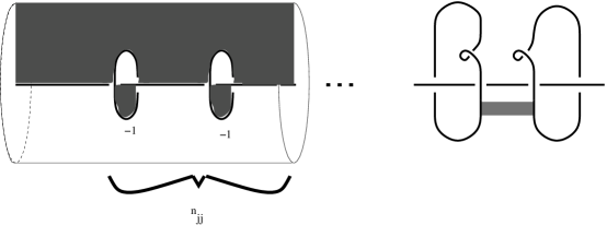
Figure 10: The $2$-cycle in the proof of Proposition 14

The boundary of $\widehat{\Sigma}_{j}$ is exactly the relation, $n_{jk}\mu_{j}=0$. The framing on each copy of $\mu_{k}$ for $k\neq j$ induced from this surface agrees with the $0$-framing. The framing on each copy of $\mu_{j}$ is $-\hbox{sign}(n_{jj})$. The surface, $\widehat{\Sigma}_{j}$ may be extended to a surface in $M\times[0,1]\times[0,1]$ by adding a collar of the boundary in the direction of the second interval followed by one band for each pair of the $\mu_{j}$ as depicted on the right of figure 10. The resulting surface has a canonical framing, and the corresponding homotopy given by the Pontrjagin-Thom construction homotopes the loop corresponding to the relation to a loop corresponding to a $\pm 2$-framed unlink. Such a loop is null-homotopic, as required. $\Box$

We remark that the Spin structures on $M$ correspond to $H^{1}(M;{\mathbb{Z}}_{2})$. In addition, the splittings of ${\mathbb{Z}}_{2}\to\pi_{1}(\hbox{Sp}(1)^{M})\to H^{2}(M;{\mathbb{Z}})$ corresponds to the group cohomology,

$$H^{1}(H^{2}(M;{\mathbb{Z}});{\mathbb{Z}}_{2})\cong H^{1}(H_{1}(M;{\mathbb{Z}});{\mathbb{Z}}_{2})\cong H^{1}(M;{\mathbb{Z}}_{2}).$$

The last isomorphism is because the $2$-skeleton of $M$ is the $2$-skeleton of a $K(H_{1}(M;{\mathbb{Z}}),1)$. A combination of Propositions 13 and 14 together with Reductions 5, 6 and 7 and the corollary of the universal coefficient theorem that $H^{*}(X;A\oplus B)\cong H^{*}(X;A)\oplus H^{*}(X;B)$ give Theorem 2.

6.2 Cohomology of Skyrme configuration spaces

As we have seen we may restrict our attention to compact, simple, simply-connected $G$. Recall the cohomology classes, $x_{j}$, and the $\mu$-map defined in section 4. Throughout this section we will take the coefficients of any homology or cohomology to be the real numbers unless noted to the contrary. To compute the cohomology of $G^{M}$ we will use the cofibrations $M^{(k)}\to M^{(k+1)}\to M^{(k+1)}/M^{(k)}$ and the fact that $M^{(k+1)}/M^{(k)}$ is a bouquet of spheres to reduce the problem to the case where the domain is a sphere.

Briefly recall the computation of the cohomology of the loop spaces. These are well known results, but we sketch a proof because this explains why the classes $\mu(\Sigma,x_{j}x_{k})$ are trivial. As usual let $\Omega^{k}G=G^{S^{k}}$ denote the $k$-iterated loop space. We have the following lemma.

Lemma 15

The cohomology rings of the first loop groups are given by, $H^{*}(\Omega G)={\mathbb{R}}[\mu([S^{1}]\otimes x_{j})]$, $H^{*}(\Omega^{2}G)={\mathbb{R}}[\mu([S^{2}]\otimes x_{j})]$, and $H^{*}(\Omega^{3}_{0}G)={\mathbb{R}}[\mu([S^{3}]\otimes x_{j}),j>3]$.

Proof:  Recall that the path space, $PG$ is contractible, and fits into a fibration, $\Omega G\hookrightarrow PG\to G$. The Serre spectral sequence of this fibration has, $E_{2}^{p,q}=H^{p}(G;H^{q}(\Omega G))$. Since $G$ is simply-connected, the coefficient system is untwisted. Since $PG$ is contractible all classes of positive degree have to die at some point in this spectral sequence. By location we know that all differentials of $x_{3}$ vanish, so there must be some class in $H^{2}(\Omega G)$ mapping to $x_{3}$. The class $\mu([S^{1}]\otimes x_{3})$ is one such class, and the only class that there can be without having something else live to the limit group of the spectral sequence. Notice that classes of the form $x_{3}\prod x_{j_{k}}$ are images of classes of the form $\mu([S^{1}]\otimes x_{3})\prod x_{j_{k}}$, so we have killed all classes with a factor of $x_{3}$. In the same way, we can kill terms with a factor of the next $x_{j}$. We conclude that $H^{*}(\Omega G)={\mathbb{R}}[\mu([S^{1}]\otimes x_{j})]$. Repeating the argument with the fibration, $\Omega^{2}G\to P\Omega G\to\Omega G$ we obtain, $H^{*}(\Omega^{2}G)={\mathbb{R}}[\mu([S^{2}]\otimes x_{j})]$. This time the coefficient system is untwisted because, $\pi_{1}(\Omega G)\cong\pi_{2}(G)=0$.

We need to adjust the argument a bit at the next stage because $\pi_{0}(\Omega^{3}G)\cong\pi_{1}(\Omega^{2}G)\cong\pi_{3}(G)\cong{\mathbb{Z}}$. This shows that the path components of $\Omega^{3}G$ may be labeled by the integers. Each component is homeomorphic to the identity component since $\Omega^{3}G$ is a topological group. In this case, we have no guarantee that the coefficient system is untwisted, so we will use a different approach that we be useful again in section 6.4. Let $\widetilde{\Omega^{2}G}$ denote the universal cover of $\Omega^{2}G$ and let $\Omega_{0}^{3}G$ denote the identity component of $\Omega^{3}G$. These fit into a fibration, $\Omega_{0}^{3}G\to P\widetilde{\Omega^{2}G}\to\widetilde{\Omega^{2}G}$ that may be used to obtain, $H^{*}(\Omega^{3}_{0}G)={\mathbb{R}}[\mu([S^{3}]\otimes x_{j}),j>3]$. We will use equivariant cohomology to compute the cohomology of $\widetilde{\Omega^{2}G}$.

Recall that any Lie group, say $\Gamma$, acts properly on a contractible space called the total space of the universal bundle. This space is denoted $E\Gamma$. The quotient of this by $\Gamma$ is the classifying space $B\Gamma$. Let $X$ be a $\Gamma$ space (i.e. a space with a $\Gamma$ action) and consider the space $X_{\Gamma}:=E\Gamma\times_{\Gamma}X$. The cohomology of the space $X_{\Gamma}$ is called the equivariant cohomology of $X$. It is denoted by $H^{*}_{\Gamma}(X)$. When the $\Gamma$ action on $X$ is free and proper (as it is in our case), we have a fibration $X_{\Gamma}\to X/\Gamma$ obtained by ignoring the $E\Gamma$ component in the definition of $X_{\Gamma}$. The fiber of this fibration is just $E\Gamma$ which is contractible, so the spectral sequence of the fibration implies that the cohomology of $X/\Gamma$ is isomorphic to the equivariant cohomology of $X$. By ignoring the $X$ component in the definition of $X_{\Gamma}$ we obtain a fibration $X_{\Gamma}\to B\Gamma$ that may be used to relate the equivariant cohomology of $X$ to the cohomology of $X$.

If we apply these ideas with $X=\widetilde{\Omega^{2}G}$ and $\Gamma=\pi_{1}(\Omega^{2}G)\cong{\mathbb{Z}}$, we obtain a spectral sequence that may be used to show that the cohomology of $\tilde{\Omega^{2}G}$ is generated by $\mu([S^{2}]\otimes x_{j})$ for $j>3$. This then plugs in to give the stated result for $\Omega^{3}_{0}G$. $\Box$

Returning to the situation of a $3$-manifold domain, let $M$ have a cell decomposition with one $0$-cell ($p_{0}$) several $1$-cells ($e_{r}$) several $2$-cells ($f_{s}$) and one $3$-cell ($[M]$). Since $G^{X\vee Y}=G^{X}\times G^{Y}$, and $M^{(k+1)}/M^{(k)}$ is a bouquet of spheres we have,

$$\begin{array}[]{rcl}H^{*}(G^{M^{(1)}})&=&{\mathbb{R}}[\mu(e_{r}\otimes x_{j})],\\ H^{*}(G^{M^{(2)}/M^{(1)}})&=&{\mathbb{R}}[\mu(f_{s}\otimes x_{j})],\\ H^{*}(G^{M^{(3)}/M^{(2)}}_{0})&=&{\mathbb{R}}[\mu([M]\otimes x_{j}),j>0].\end{array}$$

The next lemma assembles these facts into the cohomology of $G^{M^{(2)}}$.

Lemma 16

If $\Sigma^{1}_{r}$ form a basis for $H_{1}(M)$, and $\Sigma^{2}_{s}$ form a basis for $H_{2}(M)$ we have,

$$H^{*}(G^{M^{(2)}})={\mathbb{R}}[\mu(\Sigma^{1}_{r}\otimes x_{j}),\mu(\Sigma^{2}_{s}\otimes x_{k})].$$

Proof:  The cofibration $M^{(1)}\to M^{(2)}\to M^{(2)}/M^{(1)}$ leads to a fibration,

$$G^{M^{(2)}/M^{(1)}}\to G^{M^{(2)}}\to G^{M^{(1)}}.$$

Since $G$ is $2$-connected, $\pi_{1}(G^{M^{(1)}})=0$, so the coefficients in the cohomology appearing in the second term of the Serre spectral sequence are untwisted. We have,

$$\begin{array}[]{rcl}E_{2}^{*,*}&=&H^{*}(G^{M^{(1)}};H^{*}(G^{M^{(2)}/M^{(1)}}))\\ &=&H^{*}(G^{M^{(1)}})\otimes H^{*}(G^{M^{(2)}/M^{(1)}})\\ &\cong&{\mathbb{R}}[\mu(e_{r}\otimes x_{j}),\mu(f_{s}\otimes x_{k})].\end{array}$$

To go further we need to understand the differentials in this spectral sequence. Since $\mu(e_{r}\otimes x_{j})\in E_{2}^{j-1,0}$ we have $d_{k}\mu(e_{r}\otimes x_{j})=0$ for all $k$. We will show that $d_{\ell}\mu(f_{s}\otimes x_{k})=0$ for $\ell<k-1$ and $d_{k-1}\mu(f_{s}\otimes x_{k})=-\mu((\partial f_{s})\otimes x_{k})$ from which the result will follow. The multiplication on $G$ induces a ring structure on the homology of $G^{M^{(1)}}$ and $G^{M^{(2)}/M^{(1)}}$. Using the homology spectral sequence of the path fibrations, one may show that these homology groups are generated by cycles $e_{r}\beta_{j}:\Sigma_{r}^{j-1}\to G^{M^{(1)}}$ and $f_{s}\beta_{k}:\Sigma_{s}^{k-2}\to G^{M^{(2)}/M^{(1)}}$ dual to $\mu(e_{r}\otimes x_{j})$ and $\mu(f_{s}\otimes x_{k})$ respectively. The product in the homology ring of $G^{X}$ is given by $\beta\cdot\beta^{\prime}:\Sigma\times\Sigma^{\prime}\to G^{X}$ with $\beta\cdot\beta^{\prime}(x,y)(p)=\beta(x)(p)\beta^{\prime}(y)(p)$. The computation 4.2 in section 4 shows that the differential of our spectral sequence is given by

$$(d_{\ell}\mu(f_{s}\otimes x_{k}))(\beta\otimes\beta^{\prime})=-\int_{(\partial f_{s})\times\Sigma\times\Sigma^{\prime}}w^{*}x_{k},$$

where $w(p,x,y)=\beta(x)(p)\beta^{\prime}(y)(\pi(p))$ and $\pi:M^{(2)}\to M^{(2)}/M^{(1)}$ is the canonical projection. We are using the integral as a suggestive notation for the cap product. We see that the map $w$ factors through $(\partial f_{s})\times\Sigma\times\hbox{point}$. When $\ell<k-1$, $(\partial f_{s})\times\Sigma\times\hbox{point}$ has dimension less than $k$, so the differential is trivial. For $\ell=k-1$, this reduces to the claimed result. $\Box$

We remark that the above lemma is a valid computation of the cohomology of $G^{K}$ when $K$ is any connected $2$-complex. To go up to the next and final stage we need to analyze the action of the fundamental group of $G^{M^{(2)}}$ on the cohomology of $G^{M^{(3)}/M^{(2)}}$. This will require Lemma 12 from the beginning of this section. This is the place in the cohomology computation where we use the fact that $M$ is orientable. Let us review the situation for general fibrations first. If $F\hookrightarrow E\to B$ is a fibration and $\gamma:[0,1]\to B$ represents an element of the fundamental group of $B$ one can define a map, $\Gamma:F\times[0,1]\to B$ by $\Gamma(x,t)=\gamma(t)$. The map, $\Gamma_{0}:F\to B$ lifts to the inclusion, $F\to E$. By the homotopy lifting property, there is a lift, $\overline{\Gamma}:F\times[0,1]\to E$. The restriction, $\overline{\Gamma}_{1}:F\to F$ induces a map on the cohomology of $F$. This is how the fundamental group of the base of a fibration acts on the cohomology of the fiber. The following lemma shows that the action of the fundamental group on the cohomology of the fiber of our final fibration is trivial.

Lemma 17

If $M$ is an orientable $3$-manifold and $G$ is a compact, simply-connected Lie group then the action of $\pi_{1}(G^{M^{(2)}})$ on $H^{*}(G^{M^{(3)}/M^{(2)}})$ is trivial.

Proof:  Let $\widehat{\gamma}:SM^{(2)}\to G$ represent an element of $\pi_{1}(G^{M^{(2)}})$. By Lemma 12, this extends to a map, $\widehat{\zeta}:SM^{(3)}\to G$. Now define $\overline{\Gamma}:G^{M^{(3)}/M^{(2)}}\times[0,1]\to G^{M}$ by $\overline{\Gamma}(u,t)(x)=u([x])\widehat{\zeta}([x,t])$. The upper triangle of the following diagram commutes because $\widehat{\zeta}([x,0])=1$. The lower triangle commutes because, $\widehat{\zeta}|_{SM^{(2)}}=\widehat{\gamma}$. Thus $\overline{\Gamma}$ is an appropriate lift. Since $u([x])=1$ for $x\in M^{(2)}$, $\overline{\Gamma}_{1}$ is the identity map and the action on the cohomology of the fiber is trivial. $\Box$

We can now complete the proof of Theorem 2. The cofibration $M^{(2)}\to M^{(3)}\to M^{(3)}/M^{(2)}$ leads to a fibration,

$$G^{M^{(3)}/M^{(3)}}\to G^{M^{(3)}}\to G^{M^{(2)}}.$$

By the previous lemma, the coefficients in the cohomology appearing in the second term of the Serre spectral sequence are untwisted. Using Lemma 16, we have,

$$\begin{array}[]{rl}E_{2}^{*,*}&=H^{*}(G^{M^{(2)}};H^{*}(G^{M^{(3)}/M^{(2)}}))=H^{*}(G^{M^{(2)}})\otimes H^{*}(G^{M^{(3)}/M^{(2)}})\\ &\cong{\mathbb{R}}[\mu(\Sigma^{1}_{r}\otimes x_{j}),\mu(\Sigma^{2}_{s}\otimes x_{k}),\mu([M]\otimes x_{\ell}),\ell>0].\end{array}$$

Repeating the argument from Lemma 16 with computation 4.2, we see that all of the differentials of this spectral sequence vanish. This completes our computation of the cohomology of the Skyrme configuration space. $\Box$

6.3 The fundamental group of Faddeev-Hopf configuration spaces

In this subsection we compute the fundamental group of the Faddeev-Hopf configuration space, $(S^{2})^{M}$. Recall (Theorem 4) that the path components $(S^{2})^{M}_{\varphi}$ (where $\varphi$ is any representative of the component) fall into families labelled by $\varphi^{*}\mu_{S^{2}}\in H^{2}(M;{\mathbb{Z}})$, where $\mu_{S^{2}}$ is a generator of $H^{2}(S^{2};{\mathbb{Z}})$, and that components within a given family are labelled by $\alpha\in H^{3}(M;{\mathbb{Z}})/2\varphi^{*}\mu_{S^{2}}\smallsmile H^{1}(M;{\mathbb{Z}})$.

To analyze the Faddeev-Hopf configuration space in more detail we will further exploit its natural relationship with the classical ($G={\rm SU}(2)={\rm Sp}(1)$) Skyrme configuration space. These ideas were concurrently introduced in [5]. We identify $S^{2}$ with the unit purely imaginary quaternions, and $S^{1}$ with the unit complex numbers. The quotient, Sp$(1)/S^{1}$ is homeomorphic to $S^{2}$, with an explicit homeomorphism given by $[q]\mapsto qiq^{*}$. Our main tool will be the map

$${\mathfrak{q}}:S^{2}\times S^{1}\to\hbox{Sp}(1),\qquad{\mathfrak{q}}(x,\lambda)=q\lambda q^{*},\qquad\hbox{where}\ x=qiq^{*}.$$ (6.2)

It is not difficult to verify the following properties of ${\mathfrak{q}}$.

1. It is well defined and smooth.

2. ${\mathfrak{q}}(x,\lambda_{1}\lambda_{2})={\mathfrak{q}}(x,\lambda_{1}){\mathfrak{q}}(x,\lambda_{2})$.

3. ${\mathfrak{q}}^{-1}(1)=S^{2}\times\{1\}$.

4. ${\mathfrak{q}}(x,\lambda)x({\mathfrak{q}}(x,\lambda))^{*}=x$.

5. ${\mathfrak{q}}(x,\cdot):S^{1}\to\{q|qxq^{*}=x\}$ is a diffeomorphism.

6. deg$({\mathfrak{q}})=2$ with the standard “outer normal first” orientations.

For example writing $x=qiq^{*}$, the fourth property may be verified as ${\mathfrak{q}}(x,\lambda)x({\mathfrak{q}}(x,\lambda))^{*}=q\lambda q^{*}qiq^{*}q\lambda^{*}q^{*}=x$. We will let $\lambda^{x}$ denote the inverse to ${\mathfrak{q}}(x,\cdot)$. We will also use the related maps, $\rho:S^{2}\times\hbox{Sp}(1)\times S^{1}\to S^{2}\times\hbox{Sp}(1)$ and $f:S^{2}\times\hbox{Sp}(1)\to S^{2}\times S^{2}$ defined by $\rho(x,y,\lambda)=(x,y{\mathfrak{q}}(x,\lambda))$ and $f(x,q)=(x,qxq^{*})$. Properties (2) and (3) show that $\rho$ is a free right action. Properties (4) and (5) show that $f$ is a principal fibration with action $\rho$. As our first application of these maps we show that the evaluation map is a fibration.

Lemma 18

The evaluation map,

$$\hbox{ev}_{p_{0}}:\hbox{FreeMap}(M,S^{2})\to S^{2},$$

given by $\hbox{ev}_{p_{0}}(\varphi)=\varphi(p_{0})$ is a fibration.

Proof:  We just need to construct the diagonal map in the following diagram. If we define the horizontal maps in the following diagram by $\mu(x,t)=(\overline{h}(x)(p_{0}),H(x,t))$ and $\overline{\nu}(x)=(\overline{h}(x)(p_{0}),1)$, then the existence of the diagonal map will follow because $f$ is a fibration. The desired map is just, $\overline{H}(x,t)(p)=\overline{\mu}_{2}(x,t)\overline{h}(x)(p)(\overline{\mu}_{2}(x,t))^{*}$ $\Box$

Clearly the fiber of this fibration is $(S^{2})^{M}$. Recall that we are using $(S^{2})^{M}_{\varphi}$ to denote the $\varphi$-component of the space of based maps.

In [5] these ideas were used to give a new proof of Pontrjagin’s homotopy classification of maps from a $3$-manifold to $S^{2}$. The following lemma comes from that paper. A second proof of this lemma may be found in [6].

Lemma 19 (Auckly-Kapitanski)

There exists a map $u:M\to\hbox{Sp}(1)$ such that $\psi:M\to S^{2}$ and $\varphi:M\to S^{2}$ are related by $\psi=u\varphi u^{*}$ if and only if $\psi^{*}\mu_{S^{2}}=\varphi^{*}\mu_{S^{2}}$.

Theorem 5 follows directly from this lemma. Assuming $\psi^{*}\mu_{S^{2}}=\varphi^{*}\mu_{S^{2}}$, define a map $F:(S^{2})^{M}_{\varphi}\to(S^{2})^{M}_{\psi}$ by $F(\xi)=u\xi u^{*}$. This is clearly well defined because any map homotopic to $\varphi$ will be mapped to a map homotopic to $\psi$ under $F$. There is a well-defined inverse given by $F^{-1}(\zeta)=u^{*}\zeta u$.

We have a fibration relating the identity component of the Skyrme configuration space to any component of the Faddeev-Hopf configuration space.

Lemma 20

The map induced by $f$,

$$\{\varphi\}\times\hbox{Sp}(1)^{M}_{0}\stackrel{{\scriptstyle f^{*}}}{{\rightarrow}}\{\varphi\}\times(S^{2})^{M}_{\varphi}$$

is a fibration.

Proof:  Once again we just need to construct the diagonal map in a diagram. So once again we consider a second diagram. Here the horizontal maps are given by $\overline{\nu}(p,x)=(\varphi(p),\overline{h}(x)(p))$ and $\mu(p,x,t)=(\varphi(p),H(x,t)(p))$. The diagonal lift exists because $f$ is a fibration. We need to use property (5) of ${\mathfrak{q}}$ to adjust the base points. Let $x_{0}$ be the basepoint of $S^{2}$ and define the desired lift by

$$\overline{H}(x,t)(p)=\overline{\mu}_{2}(p,x,t){\mathfrak{q}}(\varphi(p),\lambda^{x_{0}}(\overline{\mu}_{2}(p,x,t)^{-1}).$$

This completes the proof. $\Box$

By property (5) of ${\mathfrak{q}}$, we see that any element of the fiber of the above fibration may be written in the form ${\mathfrak{q}}(\varphi,\lambda)$ for some map $\lambda:M\to S^{1}$. Since ${\mathfrak{q}}(\varphi,\lambda)$ is null homotopic, its degree must be zero. By property (6) of ${\mathfrak{q}}$, this implies that $\lambda^{*}\mu_{S^{1}}$ must be in the kernel of the cup product $2\varphi^{*}\mu_{S^{2}}\smallsmile$. Conversely, given any map $\lambda$ with $\lambda^{*}\mu_{S^{1}}\in\hbox{ker}(2\varphi^{*}\mu_{S^{2}}\smallsmile)$ we get an element of the fiber. Recall that the components of the space of maps from $M$ to $S^{1}$ correspond to $H^{1}(M;{\mathbb{Z}})$ and each component is homeomorphic to the identity component which is homeomorphic to ${\mathbb{R}}^{M}$ which is contractible. It follows that up to homotopy Sp$(1)^{M}_{0}$ is a regular ker$(2\varphi^{*}\mu_{S^{2}}\smallsmile)$ cover of $(S^{2})^{M}_{\varphi}$ (the fiber is homotopy equivalent to ker$(2\varphi^{*}\mu_{S^{2}}\smallsmile)$). The homotopy sequence of the fibration then gives us the following sequence:

$$0\to\pi_{1}(\hbox{Sp}(1)^{M})\to\pi_{1}((S^{2})^{M}_{\varphi})\to\hbox{ker}(2\varphi^{*}\mu_{S^{2}}\smallsmile)\to 0.$$ (6.3)

Since we do not already know that $\pi_{1}((S^{2})^{M}_{\varphi})$ is abelian, we not only need to show that the sequence splits, we also need to show that the image of the splitting commutes with the image of $\pi_{1}(\hbox{Sp}(1)^{M})$. This is the content of the following lemma. This lemma will complete the proof of Theorem 6.

Lemma 21

The sequence (6.3) splits and the image of the splitting commutes with the image of $\pi_{1}(\hbox{Sp}(1)^{M})$.

Proof:  Given $\theta\in\hbox{ker}(2\varphi^{*}\mu_{S^{2}})$ define a corresponding map $\lambda_{\theta}:M\to S^{1}$ in the usual way, $\lambda_{\theta}(p)=e^{\int^{p}_{p_{0}}\theta}$. This induces a map, $q_{\theta}:M\to\hbox{Sp}(1)$ by $q_{\theta}(p)={\mathfrak{q}}(\varphi(p),\lambda_{\theta}(p))$. We compute the degree as follows:

$$\begin{array}[]{rl}\hbox{deg}(q_{\theta})=&\int_{M}q_{\theta}^{*}\mu_{\hbox{Sp}(1)}\\ =&2\int_{M}\varphi^{*}\mu_{S^{2}}\wedge\lambda^{*}_{\theta}\mu_{S^{1}}=2\int_{M}\varphi^{*}\mu_{S^{2}}\wedge\lambda^{*}_{\theta}=0.\end{array}$$

It follows that there is a homotopy, $\overline{H}_{\theta}$ with $\overline{H}_{\theta}(0)=1$ and $\overline{H}_{\theta}(1)=q_{\theta}$. Define the splitting by sending $\theta$ to $H_{\theta}\in\pi_{1}((S^{2})_{\varphi})$ given by $H_{\theta}(t)(p)=f(\varphi(p),\overline{H}_{\theta}(t)(p))$. To see that the image of this splitting commutes with the image of $\pi_{1}(\hbox{Sp}(1)^{M})$, let $\gamma:[0,1]\to\hbox{Sp}(1)^{M}$ be a loop and define maps $\delta_{1}$ and $\delta_{2}$ by $\delta_{1}(t,s)=\frac{2t}{s+1}$ for $t\leq\frac{1}{2}(s+1)$, $\delta_{1}(t,s)=1$ otherwise and $\delta_{2}(t,s)=1-\delta_{1}(1-t,s)$. We see that $f(\varphi,(\gamma\circ\delta_{1})\cdot(\overline{H}_{\theta}\circ\delta_{2}))$ is a homotopy between $f(\varphi,\gamma)*f(\varphi,\overline{H}_{\theta})$ and $f(\varphi,\gamma\cdot\overline{H}_{\theta})$. Likewise, $f(\varphi,(\gamma\circ\delta_{2})\cdot(\overline{H}_{\theta}\circ\delta_{1}))$ is a homotopy between $f(\varphi,\overline{H}_{\theta})*f(\varphi,\gamma)$ and $f(\varphi,\gamma\cdot\overline{H}_{\theta})$. $\Box$

To prove Theorem 7, notice that we have a left $S^{1}$ action on $(S^{2})^{M}_{\varphi}$ given by $z\cdot\psi:=z\psi z^{*}$. We claim that the fibration, $\hbox{FreeMap}(M,S^{2})_{\varphi}\to S^{2},$ is just the fiber bundle with associated principal bundle Sp$(1)\to S^{2}$ and fiber $(S^{2})^{M}_{\varphi}$. In fact, the map Sp$(1)\times_{S^{1}}(S^{2})^{M}_{\varphi}\to{\mbox{FreeMaps}}(S^{2},M)$ given by $[q,\psi]\mapsto q\psi q^{*}$ is the desired isomorphism. Now consider the homotopy exact sequence of the fibration, $\hbox{FreeMap}(M,S^{2})_{\varphi}\to S^{2},$

$$\to\pi_{2}(S^{2})\to\pi_{1}((S^{2})^{M}_{\varphi})\to\pi_{1}({\mbox{FreeMaps}}(S^{2},M)_{\varphi})\to 0.$$

It follows that $\pi_{1}({\mbox{FreeMaps}}(S^{2},M)_{\varphi})$ is just the quotient of $\pi_{1}((S^{2})^{M}_{\varphi})$ by the image of $\pi_{2}(S^{2})$. The next lemma identifies this image, to complete the proof of Theorem 7.

Lemma 22

The image of the map from $\pi_{2}$ is the subgroup of $H^{2}(M;{\mathbb{Z}})<\pi_{1}((S^{2})^{M}_{\varphi})$ generated by $2\varphi^{*}\mu_{S^{2}}$.

Proof:  Recall that the map from $\pi_{2}$ of the base to $\pi_{1}$ of the fiber is defined by taking a map of a disk into the base to the restriction to the boundary of a lift of the disk to the total space. Since the boundary of the disk maps to the base point, the restriction to the boundary of the lift lies in the fiber. The homotopy exact sequence of the fibration, Sp$(1)\to S^{2}$ implies that the disk representing a generator of $\pi_{2}(S^{2})$ lifts to a disk with boundary generating the fundamental group of the fiber $S^{1}$. This lift, say $\widehat{\gamma}$ to Sp$(1)$ gives a lift $D^{2}\to\hbox{Sp}(1)\times_{S^{1}}(S^{2})^{M}_{\varphi}\cong{\mbox{FreeMaps}}(M,S^{2})$ defined by $z\mapsto[\widehat{\gamma}(z),1]$. Restricted to the boundary, this map is just $z\mapsto[z,\varphi]=[1,z\varphi z^{*}]$. It follows that the image of $\pi_{2}(S^{2})$ is just the subgroup generated by the loop $z\varphi z^{*}$. We now just have to trace this loop through the proof of the isomorphism,

$$\pi_{1}((S^{2})^{M}_{\varphi})\cong{\mathbb{Z}}_{2}\oplus H^{2}(M;{\mathbb{Z}})\oplus\hbox{\rm ker}(2\varphi^{*}\mu_{S^{2}}\smallsmile).$$

The projection to $\hbox{\rm ker}(2\varphi^{*}\mu_{S^{2}}\smallsmile)$ was defined by taking a lift of each map in the $1$-parameter family representing the loop in $\pi_{1}((S^{2})^{M}_{\varphi})$ to Sp$(1)^{M}_{0}$ and comparing the maps at the beginning and end. In our case the entire path consistently lifts to the path $\gamma_{\varphi}:S^{1}\to\hbox{Sp}(1)^{M}_{0}$ given by $\gamma_{\varphi}(z)=z{\mathfrak{q}}(\varphi,z^{*})$. It follows that the component in $\hbox{\rm ker}(2\varphi^{*}\mu_{S^{2}}\smallsmile)$ is zero. A loop such as $\gamma_{\varphi}$ naturally defines a map, $\bar{\gamma}_{\varphi}:M\times S^{1}\to\hbox{Sp}(1)$. The image of our loop in $H^{2}(M;{\mathbb{Z}})$ is just $\bar{\gamma}_{\varphi}^{*}\mu_{{\rm Sp}(1)}/[\hbox{pt}\times S^{1}]$. In notation reminiscent of differential forms this would be $\int_{{\rm pt}\times S^{1}}\bar{\gamma}_{\varphi}^{*}\mu_{{\rm Sp}(1)}$. In order to evaluate this, we write $\bar{\gamma}_{\varphi}$ as the composition of the map $(\varphi,\hbox{id}_{S^{1}}):M\times S^{1}\to S^{2}\times S^{1}$ and the map $\tilde{\mathfrak{q}}:S^{2}\times S^{1}\to\hbox{Sp}(1)$ given by $\tilde{\mathfrak{q}}(x,z)=z{\mathfrak{q}}(x,z^{*})$. This latter map is then expressed as the composition of $({\mathfrak{q}},\hbox{pr}_{2}^{*}):S^{2}\times S^{1}\to\hbox{Sp}(1)\times S^{1}$ and the map $\hbox{Sp}(1)\times S^{1}\to\hbox{Sp}(1)$ given by $(u,\lambda)\mapsto\lambda u$. The form $\mu_{{\rm Sp}(1)}$ pulls back to $\mu_{{\rm Sp}(1)}\cup 1$ under the first map, and this pulls back to $2\mu_{S^{2}}\cup\mu_{S^{1}}$ under the first factor of $\tilde{\mathfrak{q}}$ since ${\mathfrak{q}}$ has degree two. In particular $\tilde{\mathfrak{q}}$ has degree two as well. We can now complete this computation to see that our loop projects to $2\varphi^{*}\mu_{S^{2}}$ in $H^{2}(M;{\mathbb{Z}})$. To complete the proof, we need to compute the projection of our loop in the ${\mathbb{Z}}_{2}$-factor. The projection to ${\mathbb{Z}}_{2}$ is defined by multiplying the inverse of our map by the image of $2\varphi^{*}\mu_{S^{2}}$ under the splitting $H^{2}\to\pi_{1}$ and taking the framing of the inverse image of a regular point. The equivalence classes of framings may be identified with ${\mathbb{Z}}_{2}$ since the inverse image is homologically trivial. Alternatively we may compare the framing coming from our map to the framing of the map coming from the splitting. The image under the splitting of $2\varphi^{*}\mu_{S^{2}}$ is, of course, just two times the image of $\varphi^{*}\mu_{S^{2}}$ under the splitting. The inverse image coming from our map is just two copies of the inverse image of a frame under the map $(\varphi,\hbox{id}_{S^{1}}):M\times S^{1}\to S^{2}\times S^{1}$. This means that the projection is even, so zero in ${\mathbb{Z}}_{2}$. $\Box$

6.4 The cohomology of Faddeev-Hopf configuration spaces

In order to compute the cohomology of $(S^{2})^{M}_{\varphi}$ we will use the fibration, Sp$(1)^{M}_{0}\to(S^{2})^{M}_{\varphi}$. The fiber of this fibration is just ${\perp\!\!\!\perp}_{\alpha\in K}(S^{1})^{M}_{\alpha}$ where $K=\hbox{ker}(2\varphi^{*}\mu_{S^{2}}\cup)$. Up to homotopy, the fiber is just $K$. In fact we can assume that the fiber is exactly $K$ if we first take the quotient by $(S^{1})^{M}_{0}$ (which is contractible by Reduction 6). It is slightly tricky to use a spectral sequence to compute the cohomology of the base of a fibration, so we will use equivariant cohomology to recast the problem. Recall that any Lie group acts properly on a contractible space called the total space of the universal bundle. In our case, this space is denoted $EK$. The quotient of this by $K$ is the classifying space $BK$. Let $X$ be a $K$ space (i.e. a space with a $K$ action) and consider the space $X_{K}:=EK\times_{K}X$. We will be interested in the situation when $X=\hbox{Sp}(1)^{M}_{0}$ (really this divided by $(S^{1})^{M}_{0}$ but this has the same homotopy type). The cohomology of the space $X_{K}$ is called the equivariant cohomology of $X$. It is denoted by $H^{*}_{K}(X)$. When the $K$ action on $X$ is free and proper (as it is in our case), we have a fibration $X_{K}\to X/K$ obtained by ignoring the $EK$ component in the definition of $X_{K}$. The fiber of this fibration is just $EK$ which is contractible, so the spectral sequence of the fibration implies that the cohomology of $X/K$ is isomorphic to the equivariant cohomology of $X$. By ignoring the $X$ component in the definition of $X_{K}$ we obtain a fibration $X_{K}\to BK$ which may be used to compute the equivariant cohomology of $X$.

Since $H^{1}(M;{\mathbb{Z}})$ is a free abelian group, the kernel $K$ is as well. It follows that we may take $EK$ to be ${\mathbb{R}}^{n}$ with $n$ equal to the rank of $K$ and with $K$ acting by translations. It follows that $BK$ is just an $n$-torus, and we have a spectral sequence with $E_{2}$ term, $E_{2}^{p,q}=H^{p}(T^{n};\tilde{H^{q}(\hbox{Sp}(1)^{M}_{0})})$ converging to the cohomology of $(S^{2})^{M}_{\varphi}$. Clearly the fundamental group of $T^{n}$ is just $K$. To compute the action of $K$ on $H^{*}(\hbox{Sp}(1)^{M}_{0})$, let $\lambda:M\to S^{1}$ satisfy $\lambda^{*}\mu_{S^{1}}\in K$, and $\mu(\Sigma\otimes x)\in H^{q}(\hbox{Sp}(1)^{M}_{0})$ with $\sigma:\Sigma\to M$. Let $u:\Delta^{q}\to\hbox{Sp}(1)^{M}_{0}$ be a singular $q$-simplex and let $m:\hbox{Sp}(1)\times\hbox{Sp}(1)\to\hbox{Sp}(1)$ be the multiplication. Then we have,

$$\begin{array}[]{rl}(\lambda^{*}\mu_{S^{1}}\cdot\mu(\Sigma\otimes x))(u)&=\int_{\Sigma\times\Delta^{q}}m(\widehat{u},{\mathfrak{q}}(\varphi,\lambda)\circ(\sigma,1))^{*}x\\ &=\int_{\Sigma\times\Delta^{q}}(\sigma,1)^{*}{\mathfrak{q}}(\varphi,\lambda)^{*}L_{\widehat{u}}^{*}x+R_{{\mathfrak{q}}(\varphi,\lambda)\circ(\sigma,1)}^{*}\widehat{u}^{*}x\\ &=\int_{\Sigma\times\Delta^{q}}\widehat{u}^{*}x=\mu(\Sigma\otimes x)(u).\end{array}$$

Thus the fundamental group of the base acts trivially on the cohomology of the fiber. Because this fibration has an associated principal fibration with discrete group, all of the higher differentials vanish, and we obtain Theorem 8.

Theorem 9 will follow from considerations of a general fiber bundle with structure group $S^{1}$ and one computation. Let $P\to X$ be a principal $S^{1}$ bundle with simply-connected base and let $\tau:S^{1}\times F\to F$ be a left action. The Serre spectral sequence of the fibration $E=P\times_{S^{1}}F\to X$ has $E_{2}^{p,q}=H^{p}(X;{H^{q}(F;{\mathbb{R}})})$ and second differential $d_{2}\omega=c_{1}(P)\cup\tau^{*}\omega/[S^{1}]$. In our case, the principal bundle is Sp$(1)\to S^{2}$. It follows immediately that the coefficient system in the $E_{2}$ term of the Serre spectral sequence is untwisted, and that the only non-trivial differential is the $d_{2}$ differential. In this case, the first Chern class is $\mu_{S^{2}}$. The action that we consider is the map $\tau:S^{1}\times(S^{2})^{M}_{\varphi}$ given by $\tau(z,u)=zuz^{*}$. In fact, we only need to consider the effect of this action on terms coming from Sp$(1)^{M}_{0}$. This is because the action is trivial on the classes coming from $BK$. This can be seen by considering a map from $(S^{2})^{M}_{\varphi}$ to $BK$. However, the easiest way to see this is first to compute the cohomology of the fiber bundle with fiber Sp$(1)^{M}_{0}$, and then recognize that, up to homotopy, the total space of this bundle is a regular $K$-cover of ${\mbox{FreeMaps}}(M,S^{2})_{\varphi}$. Either way, we need to compute the second differential coming from the action, $\tau_{0}:S^{1}\times\hbox{Sp}(1)^{M}_{0}\to\hbox{Sp}(1)^{M}_{0}$ given by $\tau_{0}(z,u)=\tilde{\mathfrak{q}}(\varphi,z)u$. Let $u:F\to\hbox{Sp}(1)^{M}_{0}$ be a singular chain and compute

$$\left(\tau_{0}^{*}\mu(\Sigma\otimes x)/[S^{1}]\right)(u)=\int_{S^{1}\times\Sigma\times F}\left(m\circ(\tilde{\mathfrak{q}}(\varphi\circ\sigma,\hbox{pr}_{S^{1}}),\widehat{u}\circ(\sigma,\hbox{pr}_{F})\right)^{*}x.$$

Here $m:\hbox{Sp}(1)\times\hbox{Sp}(1)\to\hbox{Sp}(1)$ is multiplication, and the rest of the maps are as in the definition of $\mu(\Sigma\otimes x)$ in line 4.1. This vanishes for dimensional reasons when $\Sigma$ is a $1$-cycle ($\varphi\circ\sigma$ would push it forward to a $1$-cycle in $S^{2}$). When $\Sigma$ is a $2$-cycle, we use the product rule and the fact that $\tilde{\mathfrak{q}}:S^{2}\times S^{1}\to\hbox{Sp}(1)$ has degree two to conclude that $\left(\tau_{0}^{*}\mu(\Sigma\otimes x)/[S^{1}]\right)=2\varphi^{*}\mu_{S^{2}}[\Sigma]$. This completes the proof of our last theorem.

References

• [1] Aitchison, I. J. R.: Effective Lagrangians and soliton physics I: derivative expansion, and decoupling. Acta Phys. Polon. B18:3, 191-205 (1987)
• [2] Aitchison, I. J. R.: Berry phases, magnetic monopoles, and Wess-Zumino terms or how the Skyrmion got its spin. Acta Phys. Polon. B18:3, 207-235 (1987)
• [3] Adams, J. F.: Lectures on exceptional Lie groups. Chicago and London: The University of Chicago Press, 1996
• [4] Auckly, D., Kapitanski, L.: Holonomy and Skyrmeโ€™s Model. Commun. Math. Phys. 240, 97โ€“122 (2003)
• [5] Auckly, D., Kapitanski, L.: Analysis of the Faddeev Model. Preprint math-ph/0403025
• [6] Auckly, D., Kapitanski, L.: Integrality of invariants for Sobolev maps. In progress.
• [7] Balachandran, A., Marmo, G., Skagerstam, B., Stern, A.: Classical topology and quantum states. New Jersey : World Scientific, 1991
• [8] Balachandran, A., Marmo, G., Simoni, A., Sparno, G.: Quantum bundles and their symmetries. International J. Modern Physics A 7:8, 1641-1667 (1982)
• [9] Birrell, N., Davies, P.: Quantum fields in curved space. Cambridge: Cambridge University Press, 1982
• [10] Bopp, F., Haag, Z.: Uber die moglichkeit von spinmodellen. Zeitschrift fur Naturforschung 5a, 644 (1950)
• [11] Brรถcker, Th., tom Dieck, T.: Representation of compact Lie groups. New York : Springer-Verlag, 1985
• [12] Dirac, P.: Quantized singularities in the electromatic field. Proc. Roy. Soc. London A133, 60-72 (1931)
• [13] Dirac, P.: The theory of magnetic poles. Phys. Rev. 74, 817โ€“830 (1948)
• [14] Federer, H: A study of function spaces by spectral sequences. Ann. of Math. 61, 340-361 (1956)
• [15] Finkelstein, D., Rubinstein,J,: Connection between spin statisitics and kinks. J. Math.ย Phys. 9, 1762โ€“1779 (1968)
• [16] Giulini, D.: On the possibility of spinorial quantization in the Skyrme model. Mod.ย Phys.ย Lett. A8, 1917โ€“1924 (1993)
• [17] Gottlieb, D.: Lifting actions in fibrations. In Geometric applications of homotopy theory I. Lecture Notes in Mathematics 657, 217-253 (1978)
• [18] Halzen, F., Martin, A.: Quarks and Leptons: an introductory course in modern particle physics. New York : John Wiley and Sons (1984)
• [19] Hattori, A., Yoshida, T.: Lifting group actions in fiber bundles. Japan J. Math., 24 13-25 (1976)
• [20] Helgason, S.: Differential geometry, Lie groups and symmetric spaces. Amer. Math. Soc., Providence, Rhode Island: Amer. Math. Soc., 2001
• [21] Imbo, T.D., Shah Imbo, C., Sudarshan, E.C.G.: Identical particles, exotic statistics and braid groups. Phys.ย Lett. B 234, 103-107 (1990)
• [22] Iwasawa, K.: On some types of topological groups. Ann. of Math. 50:3, 507-558 (1949)
• [23] Kirby, R.C.: The topology of $4$-manifolds. Lecture Notes in Mathematics 1374, New York : Springer-Verlag, 1985
• [24] Krusch, S.: Homotopy of rational maps and quantization of Skyrmions. Annals Phys. 304, 103-127 (2003)
• [25] Mimura, M., Toda, H.: Topology of Lie groups, I and II. Transl. Amer. Math. Soc., Providence, Rhode Island: Amer. Math. Soc., 1991
• [26] Particle data group: Review of particle physics. http://pdg.lbl.gov
• [27] Pontrjagin, L.: A classification of mappings of the $3$-dimensional complex into the $2$-dimensional sphere. Mat. Sbornik N.S. 9:51, 331-363 (1941)
• [28] Ramadas, T. R.: The Wess-Zumino term and fermionic solitons. Commun. Math. Phys. 93, 355-365 (1984)
• [29] Schulman, L.: A path integral for spin. Phys. Rev. 176:5, 1558-1569 (1968)
• [30] Simms, D.J., Woodhouse, N.M.J.: Geometric quantization. Lecture Notes in Physics 53, Berlin: Springer-Verlag, 1977
• [31] Skyrme, T.H.R.: A unified field theory of mesons and baryons. Nucl.ย Phys. 31, 555โ€“569 (1962)
• [32] Sorkin, R.: A general relation between kink-exchange and kink-rotation. Commun. Math. Phys. 115, 421โ€“434 (1988)
• [33] Spanier, E. H.: Algebraic topology. New York: Springer, 1966
• [34] Steenrod, N.: The topology of fiber bundles. Princeton: Princeton University Press, 1951
• [35] Witten, E.: Current algebra, baryons and quark confinement. Nucl.ย Phys. B233, 433โ€“444 (1983)
• [36] Zaccaria, F., Sudarshan, E., Nilsson, J., Mukunda, N., Marmo, G., Balachandran, A.: Universal unfolding of Hamiltonian systems: from symplectic structures to fibre bundles. Phys. Rev. D27, 2327-2340 (1983)