Mechanics and Newton-Cartan-Like Gravity on the Newton-Hooke Space-time

Abstract

We focus on the dynamical aspects on Newton-Hooke space-time ${\cal NH}_{+}$ mainly from the viewpoint of geometric contraction of the de Sitter spacetime with Beltrami metric. (The term spacetime is used to denote a space with non-degenerate metric, while the term space-time is used to denote a space with degenerate metric.) We first discuss the Newton-Hooke classical mechanics, especially the continuous medium mechanics, in this framework. Then, we establish a consistent theory of gravity on the Newton-Hooke space-time as a kind of Newton-Cartan-like theory, parallel to the Newton’s gravity in the Galilei space-time. Finally, we give the Newton-Hooke invariant Schrödinger equation from the geometric contraction, where we can relate the conservative probability in some sense to the mass density in the Newton-Hooke continuous medium mechanics. Similar consideration may apply to the Newton-Hooke space-time ${\cal NH}_{-}$ contracted from anti-de Sitter spacetime.

I Introduction

From the viewpoint of purely theoretical and fundamental physics, it is well known that there are eight types of possible kinematical symmetry groups based on some rather natural assumptions Bacry . Among them the most basic two are de Sitter (dS) and anti-de Sitter (AdS) groups, which are $SO(1,d+1)$ and $SO(2,d)$ for $(1+d)$-dimensional spacetime, respectively; all the others are Inönü-Wigner contractions IW of them. The so-called Newton-Hooke (NH) group $N_{\pm}$ is an important and interesting contraction of dS/AdS group, respectively. It is the meaningful non-relativistic limit of dS/AdS group. At the same time, the Galilei group is a further contraction (the flat limit) of both $N_{\pm}$ groups. All these kinematical groups can lead to the corresponding $(1+d)$-dimensional space-times as some homogeneous spaces of them. Furthermore, the action of these groups on their corresponding space-times can take some nice fractional linear forms under special coordinate systems (called Beltrami coordinates), and the corresponding mechanics, like Newtonian mechanics on Galilei space-time, can be really established from first principles GHTXZ ; GHTXZ4 . Especially, the NH case as a non-relativistic cosmological kinematics is studied in detail in DD and recently in GHTXZ .

On the other hand, from the viewpoint of modern physics and cosmology, constant curvature space-times have drawn much attention, from both theoretical and observational considerations. The significance of AdS space is early recognized, based upon the fact that its symmetry algebra has supersymmetric extensions and so it can be incorporated into supergravity and string theory. Related study has resulted in the profound AdS/CFT correspondence AdS/CFT . The great interest in dS space comes from recent cosmological observations showing that our universe is asymptotic dS, i.e., with a positive cosmological constant 90s ; WMAP . However, there will be lots of puzzles within the present framework of physics if our universe does have a positive cosmological constant puzzle . Under this embarrassed situation, of course, any instructive attempts related to these problems are worthwhile. One available attempt is just to consider the non-relativistic limit, i.e., the NH limit, which drastically simplifies the analysis while still taking the effects of cosmological constant into account. That is why the interest in NH space-time revives recent years ABCP ; Gao ; GP ; GHTXZ .

Following our recent paper GHTXZ that investigates NH space-time from the geometric contraction, in this paper we focus on the dynamical aspects on NH space-time. We discuss in detail the NH kinematics, dynamics and even continuous medium mechanics. Especially, we establish a consistent theory of gravity on NH space-time as a kind of Newton-Cartan-like theory, parallel to the Newton’s gravity on the Galilei space-time. We also discuss some interesting aspects of the NH invariant Schrödinger equation. We find that it is possible to relate the conservative probability in some sense to the mass density in the NH continuous medium mechanics. Unlike most of preceding articles, which investigate NH mechanics mainly from the algebraic point of view, our discussion will be more geometric and based on the foundation of physics. The invariance of physics under the action of NH group plays an important role in our discussion.

The paper is organized as follows. In Sec.II, after a brief introduction to algebraic construction of NH space-time, we introduce the geometric description of dS/AdS spacetime, Beltrami coordinates, dS/AdS group action and their NH limit for the dS spacetime. In Sec.III we discuss the NH mechanics, concentrating on the dynamics. The Newton-Cartan-like theory on NH space-time is constructed in Sec.IV. We give the gravitational field equation there and solve it to obtain the law of gravity for the exterior of spherical source. In Sec.V we deduce the Schrödinger equation on NH space-time from the geometric contraction, show its NH invariance, and discuss the conservation of probability, which can be related in some sense to the mass density in fluid mechanics. We end the paper with a brief conclusion and discussion in Sec.VI.

II Newton-Hooke Space-time as a Limit of Beltrami-de Sitter Spacetime

The Lie algebra of dS/AdS group, in terms of the time-space decomposition, is (taking $d=3$ for definiteness) GHTXZ

$$[{\bf J}_{i},{\bf H}]=0,\quad[{\bf J}_{i},{\bf J}_{j}]=\epsilon_{ijk}\mathbf{J}_{k},\quad[{\bf J}_{i},{\bf P}_{j}]=\epsilon_{ijk}\mathbf{P}_{k},$$

$$[{\bf J}_{i},{\bf K}_{j}]=\epsilon_{ijk}\mathbf{K}_{k},\quad[{\bf H},{\bf P}_{i}]=\pm\nu^{2}\mathbf{K}_{i},\quad[{\bf H},{\bf K}_{i}]=\mathbf{P}_{i},$$ (1)

$$[{\bf P}_{i},{\bf P}_{j}]=\pm R^{-2}\epsilon_{ijk}\mathbf{J}_{k},\quad[{\bf K}_{i},{\bf K}_{j}]=-c^{-2}\epsilon_{ijk}\mathbf{J}_{k},\quad[{\bf P}_{i},{\bf K}_{j}]=c^{-2}\delta_{ij}\mathbf{H},$$

where the generators have their usual meanings, $\nu:=c/R$ has the same dimension as frequency, and the “$+$”/“$-$” sign is for dS/AdS, respectively. The Newton-Hooke (NH) algebra $\mathfrak{n}_{\pm}(1,3)$ is the following limit (contraction) of the above dS/AdS algebra:

$$c\to\infty,\quad R\to\infty,\quad{\rm but}\quad\nu=\frac{c}{R}{\rm~{}is~{}a~{}positive,~{}finite~{}constant},$$ (2)

which reads

$$[{\bf J}_{i},{\bf J}_{j}]=\epsilon_{ijk}\mathbf{J}_{k},\quad[{\bf J}_{i},{\bf P}_{j}]=\epsilon_{ijk}\mathbf{P}_{k},$$

$$[{\bf J}_{i},{\bf K}_{j}]=\epsilon_{ijk}\mathbf{K}_{k},\quad[{\bf H},{\bf P}_{i}]=\pm\nu^{2}\mathbf{K}_{i},\quad[{\bf H},{\bf K}_{i}]=\mathbf{P}_{i},$$ (3)

$${\rm and~{}the~{}other~{}Lie~{}brackets~{}vanish.}$$

If we first replace $\mathbf{H}$ with $\mathbf{H}-\mathrm{i}mc^{2}$, where $m$ is a central element, and then perform the contraction, we will get the central extension $\mathfrak{n}_{\pm}^{\mathrm{C}}(1,3)$ of NH algebra (3):

$$[{\bf J}_{i},{\bf J}_{j}]=\epsilon_{ijk}\mathbf{J}_{k},\quad[{\bf J}_{i},{\bf P}_{j}]=\epsilon_{ijk}\mathbf{P}_{k},$$

$$[{\bf J}_{i},{\bf K}_{j}]=\epsilon_{ijk}\mathbf{K}_{k},\quad[{\bf H},{\bf P}_{i}]=\pm\nu^{2}\mathbf{K}_{i},\quad[{\bf H},{\bf K}_{i}]=\mathbf{P}_{i},$$ (4)

$$[{\bf P}_{i},{\bf K}_{j}]=-\mathrm{i}\delta_{ij}m,\quad{\rm and~{}the~{}other~{}Lie~{}brackets~{}vanish.}$$

From the spacetime point of view, the parameter $R$ in eq.(1) is the cosmic radius, which is related to the cosmological constant $\Lambda$ by $\Lambda=\pm 3R^{-2}$. Now in the NH limit the new parameter $\nu$ takes its place and has the meaning of temporal curvature. If we perform a further contraction $\nu\to 0$ (the so-called flat limit) the algebras $\mathfrak{n}_{\pm}$ and $\mathfrak{n}_{\pm}^{\mathrm{C}}$ come back to the familiar Galilei algebra $\mathfrak{gal}$ and the corresponding central extension $\mathfrak{gal}^{\mathrm{C}}$, respectively. The algebra $\mathfrak{gal}^{\mathrm{C}}$ is well known as the symmetry of non-relativistic quantum mechanics (Schrödinger equation). And it can be seen there that the central element $m$ corresponds to the mass.

The above statements on the NH limit is from the Lie algebra point of view (or after exponentiating, from the Lie group point of view). But the group aspects are far from sufficiency. The geometric aspects, such as connections, metrics (if exist) etc, are very important when concerning physics on these space-times. Conventionally, the next step is to consider dS and AdS spacetimes and NH space-time as homogeneous spaces $SO(1,d+1)/SO(1,d)$, $SO(2,d)/SO(1,d)$ and $N_{\pm}(1,d)/\hat{N}_{\pm}(1,d)$, respectively, while considering the original groups as the corresponding principal bundles over them. Here $\hat{N}_{\pm}(1,d)$ is the homogeneous NH group, whose Lie algebra is the subalgebra of $\mathfrak{n}_{\pm}(1,d)$ generated by $\mathbf{J}_{i}$ and $\mathbf{K}_{i}$. Then one can examine the actions of dS, AdS and NH groups on these homogeneous spaces. In this picture the invariant connections on these spaces can be systematically obtained as the so-called “canonical” connections KN ; ABCP . However, this picture does not help us establish the NH dynamics when taking into account the gravity from matter.

Fortunately, the dS/AdS spacetime has a simple geometric description as the pseudo-sphere embedded in higher dimensional Minkowski spacetime. The NH space-time $\mathcal{NH}_{\pm}$ can be directly obtained as some appropriate limit of this geometric picture. In fact, this naive limiting procedure can give us all the necessary geometric information of NH space-time. So, from now on, we can forget the algebraic construction of NH space-time and study $\mathcal{NH}_{\pm}$ directly from a geometric point of view. In the following, we only consider the dS case and the corresponding $\mathcal{NH}_{+}$ (denoted by $\mathcal{NH}$ for briefness). $\mathcal{NH}_{-}$ can be dealt with in parallel.

II.1 Hyperboloid Model of de Sitter Spacetime

As is well known, the 4-dimensional dS spacetime can be viewed as a hyperboloid (Fig.1)

$$\mathcal{S}_{R}:\eta_{AB}\xi^{A}\xi^{B}=-R^{2},\quad\eta_{AB}=\mathrm{diag}(1,-1,-1,-1,-1),$$ (5)

with topology $S^{3}\times\mathbb{R}$, in the 5-dimensional Minkowski spacetime $\mathbb{R}^{1,4}$. Indices $A$, $B$, etc., run over 0 to 4, while Greek indices such as $\mu$, $\nu$ run over 0 to 3.

Since $\mathcal{S}_{R}$ is invariant under the action of $O(1,4)$ on $\mathbb{R}^{1,4}$, the latter induces an action on $\mathcal{S}_{R}$. This transformation group is called the dS group. In this paper we are mainly interested in the invariant structure of dS spacetime under the action of $SO^{\uparrow}(1,4)$, the connected Lie subgroup of $O(1,4)$ that preserves the orientation and time orientation. It is denoted by $G$.

The next step is to chose some coordinate systems on the dS spacetime, which remain meaningful after the NH limit, and which admit a physical interpretation (as inertial frames, actually) and can be used to establish kinematics on dS spacetime and NH space-time. For these reasons, and in order to relate our discussion to physical principles GHTXZ in future works, we choose the Beltrami coordinates.

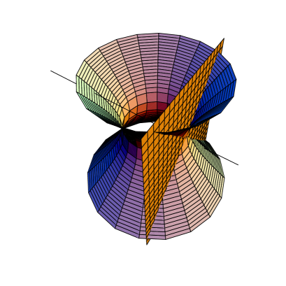
Figure 1: The hyperboloid $\mathcal{S}_{R}$ and the hyperplane $\mathcal{P}$. The Straight line passes through 0 and a pair of antipodal points in $\mathcal{S}_{R}$.

II.2 Beltrami-de Sitter Model

II.2.1 Beltrami Coordinates

Now let $\mathcal{P}_{4}^{+}$ be the hyperplane $\xi^{4}=R$ in $\mathbb{R}^{1,4}$. For each point $\xi\in\mathcal{S}_{R}$ with $\xi^{4}>0$, there is a one-to-one-corresponding point $x\in\mathcal{P}_{4}^{+}$ such that

$$\xi_{x}^{\mu}=R\frac{\xi^{\mu}}{\xi^{4}}=:x^{\mu},\quad\xi_{x}^{4}=R.$$ (6)

This map is actually obtained by drawing a straight line passing through $\xi$ and $0\in\mathbb{R}^{1,4}$, as shown in Fig.1. Since $\xi\in\mathcal{S}_{R}$ satisfies eq.(5), the corresponding $x$ in $\mathcal{P}_{4}^{+}$ satisfies

$$\sigma(x)>0,$$ (7)

where

$$\sigma(x)=1-R^{-2}\eta_{\mu\nu}x^{\mu}x^{\nu}.$$ (8)

The above “gnomonic” projection from $\mathcal{S}_{R}$ with $\xi^{4}>0$ into $\mathcal{P}_{4}^{+}$ defines a coordinate system on a patch, denoted $U_{4}^{+}$, of $\mathcal{S}_{R}$, which is known as a Beltrami coordinate system GHXZ ; GHXZ2 ; GHTXZ . Note that in order to preserve the orientation, the antipodal identification should not been taken. Under the Beltrami coordinates, the metric on $\mathcal{S}_{R}$ has the form

$$ds^{2}=[\eta_{\mu\nu}\sigma^{-1}(x)+R^{-2}\eta_{\mu\rho}\eta_{\nu\sigma}x^{\rho}x^{\sigma}\sigma^{-2}(x)]dx^{\mu}dx^{\nu}.$$ (9)

We also give the Christoffel connection

$$\Gamma^{\phantom{\mu}\rho}_{\mu\nu}=\frac{x_{\mu}\delta^{\rho}_{\nu}+x_{\nu}\delta^{\rho}_{\mu}}{R^{2}\sigma(x)}$$ (10)

of this metric for later reference.

The patch $U_{4}^{+}$ covers almost half of $\mathcal{S}_{R}$. The other half is almost covered by another patch $U_{4}^{-}$, which is the “gnomonic” projection from $\mathcal{S}_{R}$ with $\xi^{4}<0$ into the hyperplane $\mathcal{P}_{4}^{-}$ located at $\xi^{4}=-R$ in $\mathbb{R}^{1,4}$. The Beltrami coordinates on $U_{4}^{-}$ is given by

$$x^{\mu}=-R\frac{\xi^{\mu}}{\xi^{4}}.$$ (11)

Obviously, there are at least eight patches $U_{\alpha}^{\pm},\alpha=1,\cdots,4$ to cover the whole $\mathcal{S}_{R}$. In patches $U_{\alpha}^{\pm},\alpha=1,2,3$, the Beltrami coordinates are given by

$$x^{\nu}=\pm R\frac{\xi^{\nu}}{\xi^{\alpha}},\quad\nu=0,\cdots,\hat{\alpha},\cdots,4,\quad\xi^{\alpha}\gtrless 0,$$ (12)

where $\hat{\alpha}$ means omission of $\alpha$. In the following discussions, we mainly concentrate on the $U_{4}^{+}$ patch.

The 3-dimensional hyperboloid

$$\sigma(x)=0$$ (13)

is a part of the projective boundary of $\mathcal{S}_{R}$ GHTXZ4 , which corresponds to the conformal boundary on the Penrose diagram of dS spacetime. In fact, it is the intersection of $\mathcal{P}_{4}^{+}$ and the 5-dimensional light cone

$$\eta_{AB}\xi^{A}\xi^{B}=0.$$ (14)

II.2.2 Fractional Linear Form of de Sitter Group

The isometry group of $\mathcal{S}_{R}$ is $O(1,4)$. Its subgroup $SO^{\uparrow}(1,4)$ which preserves the orientation and time orientation of $\mathcal{S}_{R}$ has been denoted by $G$. Let $(D^{A}_{\ B})\in G$. Then a point $(\xi^{A})\in\mathbb{R}^{1,4}$ will be sent to another point $(\xi^{\prime A})=(D^{A}_{\ B}\,\xi^{B})$. Examples show that $D^{4}_{\ 4}$ can be arbitrary real number when $(D^{A}_{\ B})$ runs over $G$. Later we will identify the transformations in $G$ with transformations among inertial frames on dS spacetime (and its NH limit $\mathcal{NH}$).

For a given $(D^{A}_{\ B})$, if $D^{4}_{\ 4}\neq 0$, we can define

$$a_{\mu}=-R\,\frac{D^{4}_{\ \mu}}{D^{4}_{\ 4}},\qquad a^{\mu}=\eta^{\mu\nu}a_{\nu}.$$ (15)

Then we can obtain the relations

$$D^{4}_{\ 4}=\pm\sigma^{-1/2}(a),\qquad D^{\mu}_{\ 4}=-\frac{D^{\mu}_{\ \nu}\,a^{\nu}}{R}.$$ (16)

In the following, the signs $\pm$ and $\mp$ are taken corresponding to the sign of $D^{4}_{\ 4}$. We can define

$$L^{\mu}_{\ \nu}=D^{\mu}_{\ \nu}-\frac{R^{-2}\,D^{\mu}_{\ \rho}\,a^{\rho}a_{\nu}}{1+\sigma^{1/2}(a)},$$ (17)

which satisfy

$$\eta_{\rho\sigma}L^{\rho}_{\ \mu}L^{\sigma}_{\ \nu}=\eta_{\mu\nu}.$$ (18)

The inverse relation reads

$$D^{\mu}_{\ \nu}=L^{\mu}_{\ \nu}+\frac{R^{-2}\,L^{\mu}_{\ \rho}\,a^{\rho}a_{\nu}}{\sigma(a)+\sigma^{1/2}(a)}.$$ (19)

The action of $(D^{A}_{\ B})$ on $U_{4}^{+}$ can be easily obtained from eq.(6). The result takes a factional linear form:

$$\tilde{x}^{\mu}=\pm\frac{B^{\mu}_{\ \nu}(x^{\nu}-a^{\nu})}{\sigma(a,x)},$$ (20)

where

$$\sigma(a,x):=1-R^{-2}\,\eta_{\mu\nu}a^{\mu}x^{\nu},\qquad B^{\mu}_{\ \nu}:=\sigma^{1/2}(a)D^{\mu}_{\ \nu}.$$ (21)

In fact, if $\pm\sigma(a,x)>0$, $x^{\prime}$ remains in the $U_{4}^{+}$ patch and so eq.(20) is valid; if $\pm\sigma(a,x)\leq 0$, then $x^{\prime}$ will go out of $U_{4}^{+}$ and a transition between coordinate patches is needed. It is important that all transition functions in intersections can be realized by elements of $G$, which is easily understood.

II.3 The Newton-Hooke Limit

Here we choose the most convenient way to consider the NH limit from the 5-dimensional point of view. Replace for all equations in Sec.II.2 the original metric $\eta_{AB}$ with

$$g_{AB}=\mathrm{diag}(c^{2},-1,-1,-1,-1),$$ (22)

where $c$ is a positive constant with the physical meaning speed of light. Now $\xi^{0}$ has a dimension of time, and we can define

$$t\equiv x^{0}=R\xi^{0}/\xi^{4}.$$ (23)

When $c$ increases, the 5-dimensional light cone

$$g_{AB}\xi^{A}\xi^{B}=0$$ (24)

collapses. The NH limit is attained when $c,R\rightarrow\infty$ while keeping $\nu\equiv c/R$ fixed. This will keep the crossing points of the 5-d light cone and the $x^{0}$ axis on $\mathcal{P}_{4}^{+}$ fixed at $x^{0}=\pm 1/\nu$. In fact, the $c\rightarrow\infty$ limit of the original 5-d Minkowski spacetime is the 5-d Galilei space-time. The latter has a degenerate (or split) space-time metric, which induces the split metric of NH space-time $\mathcal{NH}$. Now the $U_{4}^{+}$ patch is itself geodesically complete, so other coordinate patches are no longer needed. It is easy to see that the projective boundary becomes the hyperplanes $t=\pm 1/\nu$ in $\mathcal{NH}$.

Now put the NH limit in a little more detail. Using $g_{\mu\nu}=\mathrm{diag}(c^{2},-1,-1,-1)$, eq.(8) becomes

$$\sigma(t)=1-\nu^{2}t^{2}$$ (25)

under the NH limit. From the metric $g_{\mu\nu}$ the Lorentz matrix $(L^{\mu}_{\ \nu})$ has the familiar Newtonian limit:

$$\left(\begin{array}[]{cc}L^{0}_{\ 0}&L^{0}_{\ j}\\ L^{i}_{\ 0}&L^{i}_{\ j}\\ \end{array}\right)\rightarrow\left(\begin{array}[]{cc}1&0\\ -O^{i}_{\ j}u^{j}&O^{i}_{\ j}\\ \end{array}\right),\quad O^{i}_{~{}j}\in SO(3).$$ (26)

Correspondingly, one can obtain the NH limit of $D^{\mu}_{\ \nu}$ from eq.(19):

$$D^{0}_{\ 0} \rightarrow \frac{1}{\sigma^{1/2}(t_{a})},$$ (27)

$$D^{0}_{\ j} \rightarrow 0,$$ (28)

$$D^{i}_{\ 0} \rightarrow -\frac{O^{i}_{\ j}u^{j}}{\sigma^{1/2}(t_{a})}+\frac{\nu^{2}t_{a}O^{i}_{\ j}a^{j}}{\sigma(t_{a})+\sigma^{1/2}(t_{a})}=:-O^{i}_{\ j}\hat{u}^{j},$$ (29)

$$D^{i}_{\ j} \rightarrow O^{i}_{\ j},$$ (30)

where $t_{a}\equiv a^{0}$. Hereafter, $\hat{\mbox{\boldmath$u$}}$ is renamed to $u$ for convenience.

Because the restriction to $U_{4}^{+}$ requires $D^{4}_{\ 4}>0$, we will have from eq.(20)

$$\tilde{t} = \frac{t-t_{a}}{\sigma(t_{a},t)},$$ (31)

$$\tilde{x}^{i} = \frac{\sigma^{1/2}(t_{a})}{\sigma(t_{a},t)}O^{i}_{\ j}[x^{j}-a^{j}-u^{j}(t-t_{a})].$$ (32)

Defining

$$b^{i}\equiv a^{i}-u^{i}t_{a},$$ (33)

the above transformation becomes the same form as in GHTXZ :

$$\tilde{t} = \frac{t-t_{a}}{\sigma(t_{a},t)},$$ (34)

$$\tilde{x}^{i} = \frac{\sigma^{1/2}(t_{a})}{\sigma(t_{a},t)}O^{i}_{\ j}(x^{j}-b^{j}-u^{j}t).$$ (35)

The group properties of this type of fractional linear transformations have been discussed in GHTXZ . It is important that the transformation for time coordinate is independent of space coordinates, and that the transformation for space coordinates are linear among themselves. Thus it follows that the Beltrami-time simultaneity on $\mathcal{NH}$ is absolute, i.e., independent of (inertial) reference frames, which is similar to the Newtonian space-time.

Considering the infinitesimal form of NH transformation (34,35), we can get the Beltrami-coordinate realization of (anti-Hermitian) generators of the NH algebra $\mathfrak{n}_{+}(1,3)$:

$${\bf H}=\sigma(t)\partial_{t}-\nu^{2}tx^{i}\partial_{i},$$

$${\bf P}_{i}=\partial_{i},\quad{\bf K}_{i}=t\partial_{i},$$ (36)

$${\rm and~{}the~{}usual~{}form~{}of~{}the~{}}SO(3){\rm~{}generators~{}}\mathbf{J}_{i}.$$

Then the Lie brackets (3) are easily checked.

The meaningful NH limit of eq.(9) is

$$d\tau^{2}=c^{-2}ds^{2}=\sigma^{-2}(t)dt^{2}.$$ (37)

If $d\tau^{2}$ is taken as the new line element instead of $ds^{2}$, we will have the following degenerate metric tensor:

$$g_{tt}=\sigma^{-2}(t),\qquad g_{ij}=0,\qquad g_{ti}=g_{it}=0.$$ (38)

In a fixed hypersurface of simultaneity ($dt=0$), we have

$$dl^{2}=\hat{g}_{ij}dx^{i}dx^{j},\quad\hat{g}_{ij}=\sigma^{-1}(t)\delta_{ij}.$$ (39)

A connection exists as the contraction of the Christoffel connection (10), whose nonzero coefficients are only

$$\Gamma^{\ t}_{tt}=\frac{2\nu^{2}t}{1-\nu^{2}t^{2}},\qquad\Gamma^{\ i}_{tj}=\Gamma^{\ i}_{jt}=\frac{\nu^{2}t}{1-\nu^{2}t^{2}}\delta^{j}_{i}.$$ (40)

It is pleasant to see that this connection is torsion-free, as expected, and that the corresponding curvature tensor and Ricci tensor have the following nonzero components:

$$R^{i}_{t\mu\nu}=\frac{\nu^{2}}{(1-\nu^{2}t^{2})^{2}}\,(\delta^{t}_{\mu}\delta^{i}_{\nu}-\delta^{i}_{\mu}\delta^{t}_{\nu})\quad\textrm{and}\quad R_{tt}=\frac{-3\nu^{2}}{(1-\nu^{2}t^{2})^{2}},$$ (41)

respectively. Note that eq.(41) can be directly obtained by contracting the curvature tensor and Ricci tensor on $\mathcal{S}_{R}$, and that the relation

$$R_{tt}=-3\nu^{2}g_{tt}$$ (42)

holds as expected.

It is easy to check that eqs.(37), (38), (39), (40) and (41) are all invariant under NH transformations. It can be proved that the above connection is the only one that is NH invariant and keeps $d\tau$ invariant. For details, see Appendix A. Further, under the flat limit $\nu\to 0$, all the above expressions reduce to their counterparts in the Newtonian case.

III Newton-Hooke Classical Mechanics

III.1 Newton-Hooke Kinematics

Following GHTXZ , we only list here some related results of the kinematics on NH space-time. Differentiating NH transformation (34,35) gives rise to the velocity composition law

$$\tilde{v}^{i}=\frac{O_{\ j}^{i}}{\sigma^{1/2}(t_{a})}[\sigma(t_{a},t)v^{j}-u^{j}+\nu^{2}t_{a}(x^{j}-b^{j})]$$ (43)

for $\mbox{\boldmath$v$}\equiv d\mbox{\boldmath$x$}/dt$. Differentiating again, one obtains the following transformation of (3-)acceleration:

$$\frac{d\tilde{v}^{i}}{d\tilde{t}}=\frac{\sigma^{3}(t_{a},t)}{\sigma^{3/2}(t_{a})}O^{i}_{\ j}\frac{dv^{j}}{dt}.$$ (44)

Surprisingly, the NH transformation of acceleration is much simpler than that of velocity.

Noting that the NH transformation (43) of velocity is dependent on the position $x$, we can define a new quantity

$$V^{i}\equiv v^{i}+\frac{\nu^{2}tx^{i}}{1-\nu^{2}t^{2}},$$ (45)

whose NH transformation is independent of $x$:

$$\tilde{V}^{i}=\frac{\sigma(t_{a},t)}{\sigma^{1/2}(t_{a})}O_{\ j}^{i}\Big{[}V^{j}-\frac{u^{j}}{\sigma(t)}-\frac{\nu^{2}tb^{j}}{\sigma(t)}\Big{]}.$$ (46)

We will see later that this quantity is very useful.

III.2 Newton-Hooke Dynamics

It is well-known that the gnomonic projection maps a great circle (also a geodesic) on a sphere to a straight line on the target plane. Since the dS/AdS spacetime is a pseudo-sphere (see eq.(5) for the dS spacetime), one can expect that the similar conclusion holds. This is indeed the case, and is actually an important reason why we chose such a kind of coordinate systems GHTXZ5 . Based on this, we can define the inertial motion (free motion, or moving along geodesics) as uniform-velocity motion, parallel to the corresponding concept in Newtonian mechanics and Special Relativity, and identify the Beltrami coordinates with inertial frames. The fractional linear transformation (20) preserves straight (world) lines. Then the whole mechanics on dS/AdS spacetime can be established. In fact, it is more appropriate to examine this from a projective-geometry-like point of view GHTXZ4 , which we will not dwell on in this article.

In the NH limit, one can intuitively expect from the geometric picture that via Beltrami coordinates the relation between geodesics and straight lines survives. This expectation can be strictly proved using the geodesic equation with connection (40) GHTXZ . Thus, we have the counterpart of Newton’s first law on $\mathcal{NH}$, which we call Newton-Hooke’s first law.

To go further along this direction, we first list the (conserved) non-relativistic energy and 3-momentum obtained in GHTXZ as

$$E_{\mathrm{k}} = \frac{1}{2}m\mbox{\boldmath$v$}^{2}-\frac{m\nu^{2}}{2}(\mbox{\boldmath$x$}-t\mbox{\boldmath$v$})^{2},$$ (47)

$$P = m\mbox{\boldmath$v$}.$$ (48)

Then, to justify that we can extend Newton’s second law

$$\frac{dP^{i}}{dt}=F^{i}$$ (49)

to the NH space-time, it is expected that at least one side of the above equation has good property under NH transformation (34,35). In fact, we see from eq.(48) that the transformation property of $dP^{i}/dt$ is the same as that of acceleration (44). So if we assume that the force $F^{i}$ has the same transformation property, Newton’s second law can hold on $\mathcal{NH}$, which we call Newton-Hooke’s second law.

Differentiating the kinetic energy-momentum relation

$$E_{\mathrm{k}}=\frac{1}{2m}\mbox{\boldmath$P$}^{2}-\frac{\nu^{2}}{2m}(m\mbox{\boldmath$x$}-t\mbox{\boldmath$P$})^{2}$$ (50)

obtained from eqs.(47,48), we have

$$dE_{\mathrm{k}}=(1-\nu^{2}t^{2})\mbox{\boldmath$F$}\cdot d\mbox{\boldmath$x$}+\nu^{2}t\mbox{\boldmath$x$}\cdot\mbox{\boldmath$F$}dt.$$ (51)

This can be regarded as the kinetic energy theorem in $\mathcal{NH}$. A detailed discussion on the kinetic and potential energy can be found in Appendix B.

Since the NH group $N_{\pm}(1,d)$, similar to the Galilei group, has the space-translation subgroup $\mathbb{R}^{d}$, one can expect that the conservation law of momentum (for a system of particles), or equivalently Newton’s third law, is respected in some sense. In fact, it is easy to show from the velocity composition law (43) that for a two-body system the usual definitions

$$m=m_{1}+m_{2},\qquad\mbox{\boldmath$p$}=\mbox{\boldmath$p$}_{1}+\mbox{\boldmath$p$}_{2}$$ (52)

are invariant under NH transformations, which can be generalized to many-body systems. The conservation of total momentum will lead to the reversion of acting and reacting forces, which again we call Newton-Hooke’s third law. Later we will see that for the gravitational interaction on $\mathcal{NH}$ Newton-Hooke’s third law is really respected.

III.3 On Newton-Hooke Continuous Medium Mechanics

In a general curved spacetime, we have the covariant conservation of stress-energy tensor,

$$D^{\mu}T_{\mu\nu}=g^{\mu\beta}(\partial_{\beta}T_{\mu\nu}-\Gamma^{\ \alpha}_{\mu\beta}T_{\alpha\nu}-\Gamma_{\nu\beta}^{\ \alpha}T_{\mu\alpha})=0.$$ (53)

In the present paper, we use $D^{\mu}$ denoting the covariant derivative and $\nabla$ the derivative operator in 3-space. Now considering the dS spacetime, we substitute eqs.(9,10,20) into the above equations. Under the NH limit, the temporal component of eq.(53) becomes the equation of continuity:

$$\sigma(t)\partial_{t}\frac{\varrho}{\sigma^{2}(t)}-\nu^{2}tx^{i}\partial_{i}\frac{\varrho}{\sigma^{2}(t)}-4\nu^{2}t\frac{\varrho}{\sigma^{2}(t)}+\partial_{i}\frac{\jmath^{i}}{\sigma(t)}=0,$$ (54)

where we have defined $T_{tt}=\sigma^{-2}(t)\varrho$ and $T_{it}=-c^{-2}\sigma^{-1}(t)\jmath^{i}$. Taking the NH limit of coordinate transformation law of the stress-energy tensor,

$$\tilde{T}_{\mu\nu}=\frac{\partial x^{\alpha}}{\partial\tilde{x}^{\mu}}T_{\alpha\beta}\frac{\partial x^{\beta}}{\partial\tilde{x}^{\nu}},$$ (55)

we see that $\varrho$ is a scalar under NH transformations and $\jmath$ transforms as

$$\tilde{\jmath}^{i}=\frac{\sigma(t_{a},t)}{\sigma^{1/2}(t_{a})}O_{\ j}^{i}\Big{[}\jmath^{j}-\varrho\frac{u^{j}}{\sigma(t)}-\varrho\frac{\nu^{2}tb^{j}}{\sigma(t)}\Big{]},$$ (56)

which is similar to eq.(46). If we further define

$$\hat{\rho}=\sigma^{-3/2}(t)\varrho$$ (57)

and

$$\hat{\mbox{\boldmath$j$}}=\sigma^{-3/2}(t)\mbox{\boldmath$\jmath$}-\sigma^{-5/2}(t)\nu^{2}t\mbox{\boldmath$x$}\varrho,$$ (58)

eq.(54) will become the same form

$$\partial_{t}\hat{\rho}+\nabla\cdot\hat{\mbox{\boldmath$j$}}=0$$ (59)

as in the flat spaces.

The stress-energy tensor for a perfect fluid is

$$T_{\mu\nu}=(\varrho+p)U_{\mu}U_{\nu}-pg_{\mu\nu},$$ (60)

where $U_{\mu}$ is the 4-velocity. The covariant conservation (53) gives rise to

$$U_{\mu}D^{\mu}\varrho+(\varrho+p)D^{\mu}U_{\mu} = 0,$$ (61)

$$(\varrho+p)U_{\mu}D^{\mu}U_{\nu}+(U_{\mu}U_{\nu}-g_{\mu\nu})D^{\mu}p = 0.$$ (62)

Considering the dS spacetime and taking the NH limit, we obtain from eq.(61) the same equation of continuity (59) if $\hat{\rho}$ is still given by eq.(57) and $\hat{\mbox{\boldmath$j$}}$ now given by

$$\hat{j}^{i}=\frac{\varrho v^{i}}{\sigma^{3/2}(t)}=\frac{\varrho V^{i}}{\sigma^{3/2}(t)}-\frac{\nu^{2}tx^{i}\varrho}{\sigma^{5/2}(t)},$$ (63)

where $v$ and $V$ now stand for the velocity fields of the NH perfect fluid. Comparing this expression with eq.(58), one sees that

$$\mbox{\boldmath$\jmath$}=\varrho\mbox{\boldmath$V$}$$ (64)

for NH perfect fluid, which is consistent with the fact that both sides of this equation have exactly the same NH transformation property.

It can be shown that eq.(62) becomes

$$\varrho(\partial_{t}v^{i}+v^{j}\partial_{j}v^{i})=-\sigma^{-1}(t)\partial_{i}p$$ (65)

or

$$\hat{\rho}(\partial_{t}v^{i}+v^{j}\partial_{j}v^{i})=-\sigma^{-5/2}(t)\partial_{i}p$$ (66)

under the NH limit, which is the Euler equation for a perfect fluid on $\mathcal{NH}$. It is also straightforward to check the NH invariance of this equation.

IV Newton-Cartan-Like Theory on the Newton-Hooke Space-time

It is well known that Newton’s gravity can be formulated in torsion-free affine spaces Havas ; Kunzle due to Cartan’s observation Cartan . In Sec. II.3, $\mathcal{NH}$ has been shown to be a torsion-free affine space with nonzero curvature. (See eq.(40) for the connection coefficients.) So one may naturally expect that some kind of Newton-Cartan theory can be constructed to describe the gravitational interaction on $\mathcal{NH}$. In the present section, we try to follow Cartan to set up a self-consistent Newton-Cartan-like theory of gravitational interaction on $\mathcal{NH}$. As a simple dynamical model that takes the effect of cosmological constant into account, this theory may be valuable in the study of cosmology.

To construct any self-consistent, dynamical theories on $\mathcal{NH}$, the formulation of physical laws (or in other words, dynamical equations) should be invariant under NH transformations. Note that the connection in any Newton-Cartan-like theory will not be NH invariant because in the spirit of Newton-Cartan theory matter modifies the connection on the space-time and because the NH invariant connection has been determined up to a constant (See Appendix A). Similar to the Newtonian case, it can be shown that the Newton-Cartan-like connection cannot be fully determined by the invariance of physical laws and the gravitational field equation. Therefore, in order to obtain a unique and simple description of the Newton-Cartan-like theory, what we shall do in the following is to introduce physical requirements to preserve the NH invariance of as many as possible coefficients of the connection.

IV.1 Physical Requirements and Gravitational Field Equation

Following the Newton-Cartan theory, we require that a test particle in gravitational field moves along a geodesic with respect to the Newton-Cartan-like connection. We also require, from physical considerations, that the absolute time on empty $\mathcal{NH}$ is preserved, and that Newton-Hooke’s second law is valid for gravitational action. For simplicity, the Newton-Cartan-like connection coefficients are still denoted by $\Gamma_{\mu\nu}^{\ \rho}$.

First, when the absolute time is not affected by the introduction of interactions, including gravity, we have from eq.(37)

$$\frac{d^{2}t}{d\tau^{2}}+\frac{2\,\nu^{2}t}{1-\nu^{2}t^{2}}\frac{dt}{d\tau}\frac{dt}{d\tau}=0.$$ (67)

Second, the Newton-Hooke’s second law (49) can be rewritten as

$$\frac{d^{2}x^{i}}{d\tau^{2}}=\frac{F^{i}}{m}\frac{dt}{d\tau}\frac{dt}{d\tau}-\frac{2\nu^{2}t}{1-\nu^{2}t^{2}}\frac{dt}{d\tau}\frac{dx^{i}}{d\tau}.$$ (68)

In the spirit of Cartan, the two equations may be regarded as the component ones of geodesic equation as long as what is called the Newton-Cartan-like connection is taken:

$$\Gamma_{tt}^{\ t}=\frac{2\nu^{2}t}{1-\nu^{2}t^{2}},\quad\Gamma_{tj}^{\ t}=0,\quad\Gamma_{ij}^{\ t}=0,$$ (69)

$$\Gamma_{tt}^{\ i}=-\frac{F^{i}}{m},\quad\Gamma_{tj}^{\ i}=\frac{\nu^{2}t}{1-\nu^{2}t^{2}}\delta_{j}^{i},\quad\Gamma_{jk}^{\ i}=0.$$ (70)

Compared with the NH invariant connection in Appendix A, only $\Gamma_{tt}^{\ i}$ among the Newton-Cartan-like connection coefficients have different values. Though one can easily see from Appendix A that the other coefficients are still invariant under NH transformations in spite of non-vanishing $\Gamma_{tt}^{\ i}$, one may suspect the legality of the first equation in eq.(70) because $F^{i}$ transforms under NH transformations as acceleration does (see eq.(44)) while $\Gamma_{tt}^{\ i}$ are connection coefficients and have different transformation law in general. Fortunately, they satisfy the same transformation law for NH transformations, provided the other coefficients of the connection are given as in eqs.(69,70). The transformation law of $\Gamma_{tt}^{\ i}$ under NH transformations is discussed in detail in Appendix C.

If the above connection coefficients are chosen, the proper time $\tau$ on empty $\mathcal{NH}$ is still acting as an affine parameter in a gravitational field. It can also be verified that in this case a geodesic tangent to the hypersurface of simultaneity $t=t_{0}$ at $(t_{0},\mbox{\boldmath$x$}_{0})$ will not leave this hypersurface.

For the gravitational field equation, we have three constraints: the first is that its form must be invariant under NH transformations; the second is that it must reduce to its Newtonian counterpart when $\nu\to 0$; the third is that it must reduce to the empty case (42) if there is no matter at all. Thus we can assume the following form of this equation:

$$R_{tt}=4\pi G\varrho(\mbox{\boldmath$x$},t)g_{tt}-3\nu^{2}g_{tt},$$ (71)

where $G$ is the Newton-like gravitational constant and the mass density $\varrho(\mbox{\boldmath$x$},t)$ is a scalar under NH transformations. The connection (69,70) gives the only non-vanishing components of curvature tensor

$$R_{itt}^{\ \ j}\equiv-R_{tit}^{\ \ j}=\partial_{i}\Gamma_{tt}^{\ j}-\nu^{2}(1-\nu^{2}t^{2})^{-2}\delta_{i}^{j}$$ (72)

and Ricci tensor

$$R_{tt}=\partial_{i}\Gamma_{tt}^{\ i}-3\nu^{2}(1-\nu^{2}t^{2})^{-2},$$ (73)

where the second terms of both equations coincide with the empty case (41). From eq.(71) we have the following field equation:

$$\partial_{i}\Gamma_{tt}^{\ i}=\frac{4\pi G\varrho(\mbox{\boldmath$x$},t)}{(1-\nu^{2}t^{2})^{2}}.$$ (74)

IV.2 Law of Gravity for Spherical Source

To solve eq.(74), a curl-free condition must be introduced as usual. This implies that $\Gamma_{tt}^{\ i}$ can be expressed as the gradient of a scalar potential $V$ (cf Appendix B), which is responsible to the gravity induced by compact objects:

$$\Gamma_{tt}^{\ i}(t,x)=\frac{\partial_{i}V(t,x)}{1-\nu^{2}t^{2}}.$$ (75)

Thus we have

$$\triangle V=4\pi G\varrho(\mbox{\boldmath$x$},t),$$ (76)

where $\triangle:=\hat{g}^{ij}\partial_{i}\partial_{j}$ and $\hat{g}^{ij}$ is the inverse of $\hat{g}_{ij}$ in eq.(39). This equation has the same form of Poisson equation for Newton’s gravity.

For point-like gravitational source at $X$, the mass density has the form

$$\varrho(\mbox{\boldmath$x$},t)=(1-\nu^{2}t^{2})^{3/2}M\delta^{3}(\mbox{\boldmath$x$}-\mbox{\boldmath$X$}),$$ (77)

which is an NH scalar and comes back to the Newtonian case when $\nu\to 0$. Here $M$ is the mass of the point-like source. (Such a density is consistent with the density of probability from the NH Schrödinger equation, as we can see in the next section.) For boundary condition $V\to 0$ as $|\mbox{\boldmath$x$}|\to\infty$, eq.(76) is straightforward to be solved with

$$V=-\frac{\sigma^{1/2}(t)GM}{|\mbox{\boldmath$x$}-\mbox{\boldmath$X$}|}.$$ (78)

So the connection

$$\Gamma_{tt}^{\ i}=\frac{GM}{\sigma^{1/2}(t)}\frac{x^{i}-X^{i}}{|\mbox{\boldmath$x$}-\mbox{\boldmath$X$}|^{3}}$$ (79)

and the equation of motion for the test particle is obtained as

$$\frac{d^{2}x^{i}}{dt^{2}}=-\frac{GM}{\sigma^{1/2}(t)}\frac{x^{i}-X^{i}}{|\mbox{\boldmath$x$}-\mbox{\boldmath$X$}|^{3}}.$$ (80)

Compared with the ordinary (Newton’s) law of gravity, it is interesting to see that the effect of Newton-Hooke parameter $\nu$ can be totally embodied by a time-dependent gravitational “constant” $\tilde{G}(t):=\sigma^{-1/2}(t)G$, at least from the viewpoint of particle mechanics. One can check that the form of eq.(80) is invariant under NH transformations. We also learn from this law of gravity that Newton-Hooke’s third law holds in this case.

In terms of the well-used coordinates on $\mathcal{NH}$ as homogeneous space $N_{+}(1,d)/\hat{N}_{+}(1,d)$ DD ; GP , whose relation to the Beltrami coordinates is GHTXZ :

$$\tau = \nu^{-1}\tanh^{-1}\nu t,$$ (81)

$$q^{i} = \frac{x^{i}}{\sigma^{1/2}(t)},$$ (82)

eq.(80) becomes

$$\frac{d^{2}q^{i}}{d\tau^{2}}-\nu^{2}q^{i}=-GM\frac{q^{i}-Q^{i}}{|\mbox{\boldmath$q$}-\mbox{\boldmath$Q$}|^{3}}.$$ (83)

This is exactly a particular case of the so-called Dimitriev-Zel’dovich equation DZ ; Peebles ; GP . As in the usual (Newtonian) case, the result for point-like source can be readily extended to the exterior of spherical source.

V Schrödinger Equation on the Newton-Hooke Space-time

V.1 Schrödinger Equation from Geometric Contraction

From the algebraic viewpoint, the usual Schrödinger equation can be deduced from the second Casimir operator of the extended Galilei algebra $\mathfrak{gal}^{\mathrm{C}}$. This standard method can be applied to the NH case, which is shown in Appendix D. Here we want to show how the Schrödinger equation on $\mathcal{NH}$ can be directly obtained from a geometric contraction. Rewrite the Klein-Gordon equation on dS spacetime in terms of Beltrami coordinates GHTXZ as

$$[\partial_{i}\partial_{i}-c^{-2}\partial_{t}\partial_{t}+R^{-2}(t^{2}\partial_{t}^{2}+2tx^{i}\partial_{t}\partial_{i}+x^{i}x^{j}\partial_{i}\partial_{j}+2t\partial_{t}+2x^{i}\partial_{i})]\phi=m^{2}c^{2}\sigma^{-1}\phi.$$ (84)

In order to subtract the static energy, we substitute

$$\phi=\psi(\mbox{\boldmath$x$},t)e^{-\mathrm{i}mc^{2}f(t)}$$ (85)

into the above equation and require the terms of order $c^{2}$ to cancel out, which gives the condition

$$\frac{df}{dt}=(1-\nu^{2}t^{2})^{-1}.$$ (86)

Noting eq.(37) it is easy to see $f=\tau$ and the explicit form is given by eq.(81), which makes eq.(85) of clear physical meaning. Now omitting terms of order $c^{-2}$, we obtain the following Schrödinger equation for free particle on $\mathcal{NH}$:

$$\mathrm{i}\partial_{t}\psi=\Big{[}{-\frac{\nabla^{2}}{2m}+\frac{\mathrm{i}\nu^{2}tx^{i}\partial_{i}}{\sigma(t)}-\frac{m\nu^{2}\mbox{\boldmath$x$}^{2}}{2\sigma^{2}(t)}}\Big{]}\psi.$$ (87)

The invariance of eq.(87) under NH transformations is interesting, which actually gives the realization of the extended NH group $N_{+}^{\mathrm{C}}$. For simplicity, we consider rotation, time translation, space translation and boost one by one. First, eq.(87) is obviously invariant under rotation if the wave function $\psi$ is invariant. Second, time translation (34) gives an overall factor

$$\sigma(t_{a})\sigma^{-2}(t_{a},t)$$

to eq.(87) for $\tilde{t}$ if the wave function $\psi$ keeps invariant, so eq.(87) is again invariant. Third, the NH space translation

$$\tilde{x}^{i}=x^{i}-a^{i}$$ (88)

needs some careful consideration. In fact, the wave function cannot keep invariant in this case, in contrast to that of the ordinary Schrödinger equation. It transforms as

$$\psi=\tilde{\psi}\exp[\mathrm{i}m\nu^{2}t(1-\nu^{2}t^{2})^{-1}(\mbox{\boldmath$a$}\cdot\tilde{\mbox{\boldmath$x$}}+\frac{1}{2}\mbox{\boldmath$a$}^{2})].$$ (89)

It is easy to check that its inverse transformation takes the same form, which in fact imposes strong restriction on the possible forms of the wave function transformation. The calculation to substitute eqs.(88,89) into eq.(87) and check the invariance is straightforward but a little laborious. Finally, the case of boost

$$\tilde{x}^{i}=x^{i}-u^{i}t$$ (90)

is even more complicated. Eq.(87) turns out to be invariant under this transformation when the wave function transforms as

$$\psi=\tilde{\psi}\exp[\mathrm{i}m(1-\nu^{2}t^{2})^{-1}(\mbox{\boldmath$u$}\cdot\tilde{\mbox{\boldmath$x$}}+\frac{1}{2}\mbox{\boldmath$u$}^{2}t)].$$ (91)

As expected, the wave function transformations (89) and (91) come back to their familiar forms when $\nu=0$, which gives the Galilean invariance of the ordinary Schrödinger equation. Because an arbitrary NH transformation can be composed by the above transformations, we have verified the Newton-Hooke invariance of eq.(87).

To introduce interactions into Schrödinger equation (87), one just add a term to it:

$$\mathrm{i}\partial_{t}\psi=\Big{[}{-\frac{\nabla^{2}}{2m}+\frac{\mathrm{i}\nu^{2}tx^{i}\partial_{i}}{\sigma(t)}-\frac{m\nu^{2}\mbox{\boldmath$x$}^{2}}{2\sigma^{2}(t)}+\frac{U(\mbox{\boldmath$x$},t)}{\sigma(t)}}\Big{]}\psi,$$ (92)

where $U(\mbox{\boldmath$x$},t)$ is a real scalar under NH transformations. Then one can easily check the NH invariance of this Schrödinger equation based on the above discussion.

V.2 Conservation of Probability

It is interesting to ask whether there is something for eq.(92) corresponding to the conservation of probability for the ordinary Schrödinger equation. Take the complex conjugation of eq.(92):

$$-{\rm i}\partial_{t}\psi^{*}=\Big{[}{-\frac{\nabla^{2}}{2m}-\frac{{\rm i}\nu^{2}tx^{i}\partial_{i}}{\sigma(t)}-\frac{m\nu^{2}\mbox{\boldmath$x$}^{2}}{2\sigma^{2}(t)}+\frac{U(\mbox{\boldmath$x$},t)}{\sigma(t)}}\Big{]}\psi^{*}.$$ (93)

By constructing $\sigma^{-3/2}(t)[\psi^{*}\times$(92)$-\psi\times$(93)] and rearranging it, we get

$$\partial_{t}\Big{[}{\sigma^{-3/2}(t)\,\psi^{*}\psi}\Big{]}=\nabla\cdot\Big{[}{\sigma^{-3/2}(t)\frac{{\rm i}}{2m}(\psi^{*}\nabla\psi-\psi\nabla\psi^{*})+\sigma^{-5/2}(t)\nu^{2}t(\psi^{*}\mbox{\boldmath$x$}\psi)}\Big{]}.$$

So if we define the density of probability as

$$\rho=\sigma^{-3/2}(t)\psi^{*}\psi,$$ (94)

and the flux of probability as

$$\mbox{\boldmath$j$}=\sigma^{-3/2}(t)\frac{{\rm i}}{2m}(\psi\nabla\psi^{*}-\psi^{*}\nabla\psi)-\sigma^{-5/2}(t)\nu^{2}t(\psi^{*}\mbox{\boldmath$x$}\psi),$$ (95)

we do have something like the conservation of probability:

$$\partial_{t}\rho+\nabla\cdot\mbox{\boldmath$j$}=0.$$ (96)

In fact, one can check that the expression $\frac{{\rm i}}{2m}(\psi\nabla\psi^{*}-\psi^{*}\nabla\psi)$ in eq.(95) has the same NH transformation property (56) as $\jmath$ defined in the NH continuous medium mechanics. So it is easy to see from the NH invariance of $\psi^{*}\psi$ that $\rho$ and $j$ defined here have the same NH transformation properties as $\hat{\rho}$ and $\hat{\mbox{\boldmath$j$}}$ in the NH continuous medium mechanics, respectively, and that eq.(96) can be regarded as the quantum correspondence of the equation of continuity (59). This correspondence justifies eq.(96) as the genuine equation for the conservation of probability.

VI Conclusion and Discussion

In this article we have mainly discussed the dynamical aspects on Newton-Hooke space-time and established the consistent theory of gravity on this space-time as a kind of Newton-Cartan-like theory. In our discussion, we concentrate on the geometric properties of NH space-time and the NH invariance of physics on it. We obtain the NH space-time manifold, NH transformation (34,35) and NH Schrödinger equation (92) etc directly from Inönü-Wigner contraction of their dS counterparts under the Beltrami coordinates. For the NH quantum mechanics, we find that a conservative probability can be defined and related to the mass density in NH fluid mechanics.

For NH space-time the two most useful coordinates are the Beltrami coordinates and the static coordinates, their relation being eqs.(81,82). It is interesting to see from the NH transformation (34,35) that in the Beltrami coordinates NH space-time is spatially uniform, while in the static coordinates it is temporally uniform. The Beltrami coordinates are introduced through some projective-geometry-like method GHXZ ; GHXZ2 ; GHTXZ5 . It is not strange that Beltrami-dS spacetime or NH space-time has something to do with projective geometry, since there is systematic projective-geometry-like method to deal with constant curvature spaces GHTXZ4 . If the so-called “elliptic” interpretation of dS spacetime elliptic , i.e., dS spacetime with topology $\mathcal{S}_{R}/\mathbb{Z}_{2}$, is taken, one can examine dS spacetime really from projective geometry point of view. It should be mentioned that the key difference between $\mathcal{S}_{R}$ and $\mathcal{S}_{R}/\mathbb{Z}_{2}$ is that the latter is not orientable while the former is orientable.

For the Newton-Cartan-like theory on NH space-time, unlike the previous papers that take serious the diffeomorphism invariance, we concentrate on the NH invariance and construct a theory of gravity which preserves the NH invariance of the formulation of physical laws and of as many as possible coefficients of the connection. We see from eqs.(69,70) that in the Beltrami coordinates the contributions from the cosmological background and material gravitation to the connection are completely decoupled, while in other coordinates, say the static coordinates (81,82), they are not. One can reasonably expected that Beltrami coordinate systems are the only one having this property, for there exists Newton-Hooke’s first law, i.e., the law of inertia.

The discussion in this article can be easily applied to Beltrami-AdS spacetime and the corresponding $\mathcal{NH}_{-}$. It is also readily extended to space-time dimensions other than four. Especially, our Newton-Cartan-like formalism in Sec.IV can be contracted to the Newton-Cartan theory on the Galilei space-time as the case of $\nu\to 0$.

Appendix A Newton-Hooke Invariant Connection

In this appendix, we investigate connections that are invariant under NH transformations. We shall prove that the connection (40) contracted from Beltrami-dS spacetime is the only NH invariant connection that keeps the proper time $d\tau$ invariant under NH transformations.

By the term NH invariant connection, we refer to a connection with coefficients depending on the Beltrami coordinates in the same way under NH transformations:

$$\tilde{\Gamma}_{\mu\nu}^{\ \rho}(\tilde{x})=\Gamma_{\mu\nu}^{\ \rho}(\tilde{x}),$$ (97)

while, at the same time, the transformation law

$$\tilde{\Gamma}_{\mu\nu}^{\ \rho}(\tilde{x})=\frac{\partial\tilde{x}^{\rho}}{\partial x^{\sigma}}\,\frac{\partial x^{\alpha}}{\partial\tilde{x}^{\mu}}\,\frac{\partial x^{\beta}}{\partial\tilde{x}^{\nu}}\,\Gamma_{\alpha\beta}^{\ \sigma}(x)+\frac{\partial\tilde{x}^{\rho}}{\partial x^{\sigma}}\,\frac{\partial^{2}x^{\sigma}}{\partial\tilde{x}^{\mu}\partial\tilde{x}^{\nu}}$$ (98)

is satisfied.

First, space translation {$\tilde{t}=t$, $\tilde{x}^{i}=x^{i}-b^{i}$} results in $\frac{\partial\tilde{x}^{\mu}}{\partial x^{\nu}}=\delta^{\mu}_{\nu}$ and thus $\tilde{\Gamma}_{\mu\nu}^{\ \rho}(\tilde{x})=\Gamma_{\mu\nu}^{\ \rho}(x)$ according to eq.(98). Substituting it into eq.(97), we immediately obtain $\Gamma_{\mu\nu}^{\ \rho}(t,\mbox{\boldmath$x$}-\mbox{\boldmath$b$})=\Gamma_{\mu\nu}^{\ \rho}(t,\mbox{\boldmath$x$}),$ which implies that each $\Gamma_{\mu\nu}^{\ \rho}$ depends on $t$ only. Next, for boosts {$\tilde{t}=t$, $\tilde{x}^{i}=x^{i}-u^{i}t$},

$$\frac{\partial\tilde{t}}{\partial t}=1,\quad\frac{\partial\tilde{t}}{\partial x^{i}}=0,\quad\frac{\partial\tilde{x}^{i}}{\partial t}=-u^{i},\quad\frac{\partial\tilde{x}^{i}}{\partial x^{j}}=\delta^{i}_{j},$$

and inversely,

$$\frac{\partial t}{\partial\tilde{t}}=1,\quad\frac{\partial t}{\partial\tilde{x}^{i}}=0,\quad\frac{\partial x^{i}}{\partial\tilde{t}}=u^{i},\quad\frac{\partial x^{i}}{\partial\tilde{x}^{j}}=\delta^{i}_{j}.$$

The transformation law (98) gives rise to

$$\tilde{\Gamma}_{tt}^{\ t}(\tilde{t}) = \Gamma_{tt}^{\ t}(t)+2\,\Gamma_{tj}^{\ t}(t)\,u^{j}+\Gamma_{ij}^{\ t}(t)\,u^{i}u^{j},$$

$$\Gamma_{tt}^{\ i}(t) = -\Gamma_{tt}^{\ t}(t)\,u^{i}+\Gamma_{tt}^{\ i}(t)+2\,\Gamma_{jt}^{\ i}(t)\,u^{j}+\Gamma_{jk}^{\ i}(t)\,u^{j}u^{k}.$$

On the other hand, the invariance of the connection indicates $\tilde{\Gamma}_{tt}^{\ t}(\tilde{t})=\Gamma_{tt}^{\ t}(\tilde{t})=\Gamma_{tt}^{\ t}(t)$ and $\tilde{\Gamma}_{tt}^{\ i}(\tilde{t})=\Gamma_{tt}^{\ i}(\tilde{t})=\Gamma_{tt}^{\ i}(t)$. These, together with the above results, imply that

$$\Gamma_{tj}^{\ t}(t) = \Gamma_{jt}^{\ t}(t)=0,\qquad\Gamma_{ij}^{\ t}(t)=0,$$ (99)

$$\Gamma_{jk}^{\ i}(t) = 0,\qquad\Gamma_{tj}^{\ i}(t)=\Gamma_{jt}^{\ i}(t)=\frac{1}{2}\,\Gamma_{tt}^{\ t}(t)\,\delta^{i}_{j}.$$ (100)

As for $\Gamma_{tt}^{\ t}(t)$, its transformation law and invariance under NH time translation indicate

$$\Gamma_{tt}^{\ t}\left(\frac{t-t_{a}}{1-\nu^{2}t_{a}\,t}\right)=\frac{(1-\nu^{2}t_{a}\,t)^{2}}{1-\nu^{2}t_{a}^{2}}\,\Gamma_{tt}^{\ t}(t)-\frac{2\nu^{2}t_{a}\,(1-\nu^{2}t_{a}\,t)}{1-\nu^{2}t_{a}^{2}}.$$ (101)

Taking the derivative of the above equation with respect to $t_{a}$ at $t_{a}=0$, then we have

$$(1-\nu^{2}t^{2})\,\frac{d\Gamma_{tt}^{\ t}}{dt}=2\nu^{2}+2\nu^{2}t\,\Gamma_{tt}^{\ t}.$$ (102)

The general solution of this ODE reads

$$\Gamma_{tt}^{\ t}(t)=\frac{2\nu^{2}t+2C\nu}{1-\nu^{2}t^{2}}$$ (103)

with $C$ the integral constant. Finally, under space rotations {$\tilde{t}=t$, $\tilde{x}^{i}=O^{i}_{\ j}\,x^{j}$}, the transformation law (98) reduces to $\tilde{\Gamma}_{tt}^{\ i}(\tilde{t})=O^{i}_{\ j}\,\Gamma_{tt}^{\ j}(t)$. Due to the invariance, we have $\Gamma_{tt}^{\ i}(t)=O^{i}_{\ j}\,\Gamma_{tt}^{\ j}(t)$ for arbitrary $(O^{i}_{\ j})\in SO(3,\mathbb{R})$. This is only possible when

$$\Gamma_{tt}^{\ i}=0.$$ (104)

The above NH invariant connection is almost the same as that (40) contracted from Beltrami-dS spacetime, except for an arbitrary integral constant $C$. It is easy to prove that the NH invariance of proper-time element $d\tau=\sigma^{-1}(t)dt$ requires $C=0$, because the first integral of the temporal component of the geodesic equation

$$\frac{d^{2}t}{d\tau^{2}}+\Gamma_{\mu\nu}^{\ t}(t,x)\frac{dx^{\mu}}{d\tau}\frac{dx^{\nu}}{d\tau}=0$$ (105)

is

$$\frac{dt}{d\tau}=(1-\nu^{2}t^{2})\left(\frac{1-\nu t}{1+\nu t}\right)^{C},$$ (106)

which leads to $C=0$.

Appendix B Energy in Newton-Hooke Mechanics

In our formulism, the manifest time-translation invariance is lost. However, since there is “timelike” Killing vector $\mathbf{H}$ (36) in $\mathcal{NH}$ (which is $\partial_{\tau}$ in terms of the coordinates (81,82), actually), we can expect that some kind of energy conservation law should exist. Before investigating the energy conservation law, we first give some justifications for the kinetic energy (47) obtained from contraction of Beltrami-dS spacetime in GHTXZ . Under coordinate transformation (81,82) it becomes

$$E_{\mathrm{k}}=\frac{m}{2}\Big{(}\frac{d\mbox{\boldmath$q$}}{d\tau}\Big{)}^{2}-\frac{1}{2}m\nu^{2}\mbox{\boldmath$q$}^{2},$$ (107)

which is just the (conservative) total energy of an anti-harmonic oscillator, as is well known as the conservative energy in (empty) $\mathcal{NH}$ DD ; Gao . It has obvious $\tau$-translational invariance. For its full NH transformation property, we can consider $\mbox{\boldmath$v$}^{2}-\nu^{2}(\mbox{\boldmath$x$}-\mbox{\boldmath$v$}t)^{2}$ from eq.(47). A lengthy but straightforward calculation gives

$$\tilde{\mbox{\boldmath$v$}}^{2}-\nu^{2}(\tilde{\mbox{\boldmath$x$}}-\tilde{\mbox{\boldmath$v$}}\tilde{t})^{2}=(\mbox{\boldmath$v$}-\mbox{\boldmath$u$})^{2}-\nu^{2}(\mbox{\boldmath$x$}-\mbox{\boldmath$b$}-\mbox{\boldmath$v$}t)^{2},$$ (108)

which is elegant and whose $t_{a}$-independence is what we wanted.

Let us write down the total energy $E$ as

$$E=E_{\mathrm{k}}+V,$$ (109)

where $V$ is the potential energy. We require the conservation of $E$ along the world line, which gives from eq.(51)

$$\frac{dE}{dt}=[(1-\nu^{2}t^{2})F^{i}+\partial_{i}V]\frac{dx^{i}}{dt}+(\nu^{2}tx^{i}F^{i}+\partial_{t}V)=0.$$ (110)

Since this equation is valid for arbitrary $d\mbox{\boldmath$x$}/dt$, we will have

$$(1-\nu^{2}t^{2})F^{i}+\partial_{i}V = 0,$$ (111)

$$\nu^{2}tx^{i}F^{i}+\partial_{t}V = 0,$$ (112)

if the velocity-independence of both $\mbox{\boldmath$F$}=\mbox{\boldmath$F$}(t,\mbox{\boldmath$x$})$ and $V=V(t,\mbox{\boldmath$x$})$ is assumed. Eq.(111) is a generalization of the usual relation $\partial_{i}V=-F^{i}$.

Thus, we have the equation

$$\frac{\partial V}{\partial t}-\frac{\nu^{2}t}{1-\nu^{2}t^{2}}x^{i}\partial_{i}V=0$$ (113)

for $V$. This PDE can be solved with general solution

$$V=V(\sigma^{-1/2}(t)\mbox{\boldmath$x$}).$$ (114)

Noticing eq.(82), it is

$$V=V(\mbox{\boldmath$q$}),$$ (115)

which is reasonable because of the manifest time-translation invariance in coordinates (81,82).

Appendix C Transformation Property of $\Gamma_{tt}^{\ k}$

It is necessary and interesting to investigate $\Gamma_{tt}^{\ k}$ in eq.(70). The $k$-$tt$ component equation of transformation law Eq.(98), the first equation of (69), and the latter two equations of (70) give

$$\tilde{\Gamma}_{tt}^{\ k}(\tilde{t},\tilde{x})=\Gamma_{tt}^{\ i}(t,x)\frac{\partial t}{\partial\tilde{t}}\frac{\partial t}{\partial\tilde{t}}\frac{\partial\tilde{x}^{k}}{\partial x^{i}}+\frac{2\nu^{2}t}{1-\nu^{2}t^{2}}\frac{\partial t}{\partial\tilde{t}}\Big{(}\frac{\partial t}{\partial\tilde{t}}\frac{\partial\tilde{x}^{k}}{\partial t}+\frac{\partial x^{i}}{\partial\tilde{t}}\frac{\partial\tilde{x}^{k}}{\partial x^{i}}\Big{)}+\frac{\partial^{2}x^{\rho}}{\partial\tilde{t}\partial\tilde{t}}\frac{\partial\tilde{x}^{k}}{\partial x^{\rho}}.$$

The second term on the RHS vanishes since

$$\frac{\partial t}{\partial\tilde{t}}\frac{\partial\tilde{x}^{k}}{\partial t}+\frac{\partial x^{i}}{\partial\tilde{t}}\frac{\partial\tilde{x}^{k}}{\partial x^{i}}=\frac{\partial\tilde{x}^{k}}{\partial\tilde{t}}=0.$$ (116)

The third term on the RHS actually includes two parts:

$$\frac{\partial^{2}t}{\partial\tilde{t}\partial\tilde{t}}\frac{\partial\tilde{x}^{k}}{\partial t}+\frac{\partial^{2}x^{i}}{\partial\tilde{t}\partial\tilde{t}}\frac{\partial\tilde{x}^{k}}{\partial x^{i}},$$ (117)

which exactly cancels each other, as shown by careful calculation. The following identity is useful to this calculation:

$$\sigma(t_{a},t)\sigma(-t_{a},\tilde{t})=\sigma(t_{a}).$$ (118)

Thus, the NH transformation of $\Gamma_{tt}^{\ k}$ has the following form:

$$\tilde{\Gamma}_{tt}^{\ k}(\tilde{t},\tilde{x})=\Gamma_{tt}^{\ i}(t,x)\frac{\partial t}{\partial\tilde{t}}\frac{\partial t}{\partial\tilde{t}}\frac{\partial\tilde{x}^{k}}{\partial x^{i}}=\frac{\sigma^{3}(t_{a},t)}{\sigma^{3/2}(t_{a})}O^{k}_{\ i}\Gamma_{tt}^{\ i},$$ (119)

which is, in fact, the same as that of acceleration (44). This justifies the first equation in eq.(70).

Appendix D Schrödinger Equation from Algebraic Viewpoint

As is well known, the familiar Schrödinger equation can be written as

$$C_{2}\psi(\mbox{\boldmath$x$},t)=2mU(\mbox{\boldmath$x$},t)\psi(\mbox{\boldmath$x$},t),$$ (120)

where $C_{2}$ is the second order Casimir operator of the central extension $\mathfrak{gal}^{\mathrm{C}}$ of Galilei algebra:

$$C_{2}=2\mathrm{i}m\mathbf{H}+\mathbf{P}^{2},$$ (121)

and $U(\mbox{\boldmath$x$},t)$ is a scalar under NH transformations. Since eq.(120) satisfies the requirement of symmetry and is rather general, the Schrödinger equation in $\mathcal{NH}$ should also be given by it. For the extended NH algebra $\mathfrak{n}_{+}^{\mathrm{C}}$, the second Casimir is

$$C_{2}=2\mathrm{i}m\mathbf{H}+\mathbf{P}^{2}-\nu^{2}\mathbf{K}^{2},$$ (122)

where the realization (36) is modified to

$$\mathbf{P}_{i}=\partial_{i}-\frac{\mathrm{i}m\nu^{2}tx^{i}}{1-\nu^{2}t^{2}},\quad\mathbf{K}_{i}=t\partial_{i}-\frac{\mathrm{i}mx^{i}}{1-\nu^{2}t^{2}}.$$ (123)

It is straightforward to check that the above realization satisfies the $\mathfrak{n}_{+}^{\mathrm{C}}$ algebra (4). After a little calculation, one obtains the Schrödinger equation on $\mathcal{NH}$ same as eq.(92).

References

• (1) H. Bacry and J.M. Lévy-Leblond, J. Math. Phys. 9 (1968) 1605; H. Bacry and J. Nuyts, J. Math. Phys. 27 (1986) 2455.
• (2) E. Inönü and E.P. Wigner, Proc. Nat. Acad. Sci. 39 (1953) 510.
• (3) C.-G. Huang, H.-Y. Guo, Y. Tian, Z. Xu and B. Zhou, Newton-Hooke Limit of Beltrami-de Sitter Spacetime, Principles of Galilei-Hooke’s Relativity and Postulate on Newton-Hooke Universal Time, [hep-th/0403013].
• (4) H.-Y. Guo, C.-G. Huang, Y. Tian, Z. Xu and B. Zhou, in preparation.
• (5) J.R. Derome and J.G. Dubois, Nuovo Cimento B 9 (1972) 351.
• (6) J. Maldacena, Adv. Theor. Math. Phys. 2 (1998) 231 [hep-th/9711200]; E. Witten, Adv. Theor. Math. Phys. 2 (1998) 253 [hep-th/9802150]; O. Aharony, S. Gubser, J. Maldacena, H. Ooguri and Y. Oz, Phys. Rept. 323 (2000) 183 [hep-th/9905111].
• (7) A.G. Riess et al, Astron. J. 116 (1998) 1009; S. Perlmutter et al, Astrophys. J. 517 (1999) 565.
• (8) C. L. Bennett et al, Astrophys. J. (Suppl.) 148 (2003) 1; M. Tegmark, et al, [astro-ph/0310723].
• (9) E. Witten, Quantum Gravity in de Sitter Space, [hep-th/0106109]; A. Strominger, String Theory and de Sitter Cosmology, Talk at the String Satellite Conference to ICM 2002. August, 2002, Beijing; R. Bousso, Adventures in de Sitter space, [hep-th/0205177].
• (10) R. Aldrovandi, A.L. Barbosa, L.C.B. Crispino and J.G. Pereira, Class. Quant. Grav. 16 (1999) 495-506 [gr-qc/9801100].
• (11) Yi-Hong Gao, Symmetries, matrices, and de Sitter gravity, [hep-th/0107067].
• (12) G.W. Gibbons and C.E. Patricot, Class. Quant. Grav. 20 (2003) 5225 [hep-th/0308200].
• (13) S. Kobayashi and K. Nomizu, Foundations of Diff. Geometry Vol. II, Chap. X, Wiley, New York (1963).
• (14) H.-Y. Guo, C.-G. Huang, Z. Xu and B. Zhou, Mod. Phys. Lett. A 19 (2004) 1701 [hep-th/0311156].
• (15) H.-Y. Guo, C.-G. Huang, Z. Xu and B. Zhou, Phys. Letts. A 331 (2004) 1 [hep-th/0403171].
• (16) H.-Y. Guo, C.-G. Huang, Y. Tian, Z. Xu and B. Zhou, On de Sitter Invariant Special Relativity and Cosmological Constant as Origin of Inertia, [hep-th/0405137].
• (17) P. Havas, Rev. Mod. Phys. 36 (1964) 938.
• (18) H.P. Künzle, Ann. Inst. Henri Poincaré A 17 (1972) 337.
• (19) É. Cartan, Ann. Scient. Éc. Norm. Sup. 40 (1923) 325; 41 (1924) 1.
• (20) N.A. Dmitriev and Ya B. Zel’dovich, Sov. Phys. JETP 18 (1964) 793.
• (21) P.J.E. Peebles, The Large-scale structure of the universe, Princeton University Press, Princeton, NJ (1980).
• (22) V. Bargmann, Ann. Math. 59 (1954) 1.
• (23) E. Schrödinger, Expanding Universes, Cambridge University Press (1956); M. Parikh, I. Savonije and E. Verlinde, Phys. Rev. D 67 (2003) 064005 [hep-th/0209120].