hep-th/0410273

FSU-TPI-08/04

ITP-UU-04/37

SPIN-04/20

Dynamical Conifold Transitions and Moduli Trapping
in M-Theory Cosmology

Thomas Mohaupt^a and Frank Saueressig^b

^aInstitute of Theoretical Physics, Friedrich-Schiller-University Jena,
Max-Wien-Platz 1, D-07743 Jena, Germany

Thomas.Mohaupt@uni-jena.de
^bInstitute of Theoretical Physics and Spinoza Institute,
Utrecht University, 3508 TD Utrecht, The Netherlands

F.S.Saueressig@phys.uu.nl

ABSTRACT

We study five-dimensional Kasner cosmologies in the vicinity of a conifold locus occurring in a time-dependent Calabi-Yau compactification of M-theory. The dynamics of M2-brane winding modes, which become light in this region, is taken into account using a suitable gauged supergravity action. We find cosmological solutions which interpolate between the two branches of the transition, establishing that conifold transitions can be realized dynamically. However, generic solutions do not correspond to transitions, but to the moduli getting trapped close to the conifold locus. This effect results from an interplay between the scalar potential and Hubble friction. We show that the dynamics does not depend on the details of the potential, but only on its overall shape.

1 Introduction

Topology change [1, 2, 3, 4] is one of the most remarkable properties of string and M-theory compactifications on special holonomy manifolds. While such changes are, by definition, discontinuous processes from the viewpoint of differential geometry, they are smooth within string theory in the sense that all observables are continuous. The usual low energy effective action (LEEA) which includes the generically massless modes of the compactification only, however, becomes discontinuous or even singular at the transition locus. It was the insight of [7] that these discontinuities or singularities can be attributed to string or brane winding modes which become massless in the transition. Following [8] we will call points in the moduli space where additional massless states occur ‘extra species points’ (ESPs). Topological phase transitions then correspond to a subclass of ESPs. In these cases the internal space develops a singularity which can be smoothed in more than one way, thereby connecting internal spaces with different topologies.

So far, topological phase transitions have mostly been discussed in terms of parametric deformations of the internal manifold. The moduli encoding these deformations appear as scalars in the LEEA and parameterize the ground state of the action. In the vicinity of a topological phase transition (or, more generally, any ESP) one obtains additional light modes which should be explicitly included in the LEEA. A program to find such ‘extended’ LEEA for topological phase transitions (and other types of ESPs) has been started in [9, 10, 11] and was recently extended to flop [12] and conifold [13, 14] transitions occurring in Calabi-Yau (CY) compactifications of M-Theory. In the latter cases the extra light modes correspond to charged matter multiplets. These originate from M2-branes wrapping the internal two-cycles which shrink to zero volume at the transition locus. Including these extra states in the extended LEEA induces a scalar potential which is uniquely determined by the geometry of the transition. This potential does not arise from switching on fluxes: it is a consequence of the presence of charged matter and supersymmetry. Therefore it is intrinsic to flop and conifold transitions.

Comparing to flops, the special feature of a conifold transition is the appearance of a new branch of the moduli space, a so-called Higgs-branch, which starts at the transition point. In terms of the LEEA the conifold transition point is the intersection point between the Coulomb and the Higgs branch of an Abelian gauge theory. Geometrically, the transition between these two branches corresponds to a topological phase transition in which the Hodge numbers (and therefore the Euler number) of the internal space changes.

Concerning the dynamics of the moduli in the vicinity of a topological phase transition only little is known, however. For M-theory compactifications on CY threefolds explicit solutions of the dimensionally reduced theory which interpolate through a flop transition either as a function of a space-like coordinate or of time have been found in [15, 16] and [17, 18], respectively. In the latter case it was thereby found that the moduli dynamically stabilize in the vicinity of the flop region. These results complement the ones of [19, 20, 21] who find that when switching on background fluxes, the remaining vacua tend to be located at ESPs.

In this paper we use a consistent truncation of the effective supergravity description for conifold transitions [13, 14] to study the dynamics of the scalar fields in the transition region. The reason why we work in five dimensions is that in this case the actions for conifold transitions are easier to construct, because the vector multiplet sector of the theory can be treated exactly [13, 14]. The generalization to four-dimensional conifold LEEA can be treated along the lines of [11]. We do not expect that the qualitative behavior of four-dimensional models will be different from the one found in this paper.

Based on the LEEA [13, 14] we find that the leading order contribution of the scalar potential is (up to the different numerical factor) given by the potential $\mathbbm{V}=\frac{1}{2}x^{2}y^{2}$ discussed in [22, 8]. In order to make contact to the analytic results obtained there, we study the dynamics of the scalar fields in both the full supergravity model and its (non-supersymmetric) leading order approximation. Within the full model we thereby obtain numerical solutions which interpolate between the Coulomb and the Higgs branch of the conifold transition. But we also observe that due to Hubble friction such transitions tend to be suppressed, while the trapping of the moduli in the transition region is favored. When comparing these results to the leading order approximation it turns out that the qualitative behavior of the solutions is the same, and therefore only depends on the shape of the potential, but not on its details. This is interesting in the context of vacuum selection, because it shows that regions of the moduli space where additional light states appear are dynamically preferred. Investigating the origin of this trapping mechanism we find that it results from an interplay between the shape of the scalar potential and Hubble friction.

These results (and those of [17, 12]) are closely related though somewhat complementary to those of [8]. There the mechanism which traps the scalar fields at ESPs is ‘quantum moduli trapping,’ which is a consequence of the quantum production of light particles occurring when the moduli pass near an ESP [8]. In contrast, the trapping mechanism discussed in our paper (and in [17, 12]) results from an interplay between the scalar potential and Hubble friction. This has been called ‘classical moduli trapping’ in [8]. In [8] these two trapping mechanisms have been compared using the results of [22]. We re-investigate this comparison based on our results and find that, once Hubble friction is taken into account, classical moduli trapping is much more efficient than found in [8].

2 The models

Our starting point is a five-dimensional Lagrangian of the form

$$\sqrt{-g}^{-1}\mathcal{L}=-\frac{1}{2}R-\frac{1}{2}g_{XY}\partial_{\mu}q^{X}\partial^{\mu}q^{Y}-\frac{1}{2}g_{xy}\partial_{\mu}\phi^{x}\partial^{\mu}\phi^{y}-\mathbbm{V}(\phi,q)\,.$$ (2.1)

Here $g$ is the determinant of the space time metric, $R$ is its Ricci scalar, $\phi^{x}$ and $q^{X}$ are scalar fields of a non-linear sigma model, taking values in target manifolds with metrics $g_{xy}$ and $g_{XY}$, respectively, and $\mathbbm{V}(\phi,q)$ is the scalar potential. Both the (truncated) supergravity description of a conifold transition [13, 14] and the five-dimensional version of the model [22, 8] are of this general form.

In the LEEA for M-theory compactified on a Calabi-Yau threefold, the scalars $\phi^{x}$ and $q^{X}$ sit in vector and hypermultiplets, respectively. In this case the indices take values $x=1,\ldots,n_{V}$ and $X=1,\ldots,4n_{H}$, where $n_{V}$ is the number of vector and $n_{H}$ the number of hypermultiplets. The full supergravity Lagrangian for conifold transitions also contains fermions and gauge fields, and some of the hypermultiplet scalars (those which come from wrapped M2-branes) are charged. In order to have a tractable problem, we consider the minimal model for a conifold transition [13, 14], containing one vector and two hypermultiplets. As explained in [13, 14] it is currently not possible to derive the metric on the hypermultiplet manifold from M-theory. However, the non-compact Wolf spaces $U(n_{H},2)/(U(n_{H})\times U(2))$ provide a consistent choice and then the M-theory charges carried by the wrapped M2-branes fix the LEEA uniquely.

Restricting the hypermultiplet scalars to their real part and setting the vector fields to zero provides a consistent truncation of the full equations of motion. Additionally taking

$${\rm Re}(u_{1})={\rm Re}(u_{2})=:q\;,\quad{\rm Re}(v_{1})={\rm Re}(v_{2})=0\,,$$ (2.2)

the dynamics of the remaining scalar fields can be derived from the Lagrangian (2.1) by substituting the scalar field metrics

$$g_{xy}=\frac{3\left(2+\phi^{2}\right)}{(2-3\phi^{2})^{2}}\;,\qquad g_{XY}=\frac{2}{\left(1-2q^{2}\right)^{2}}\;,$$ (2.3)

and the scalar potential

$$\mathbbm{V}(\phi,q)=\left(48\pi\right)^{2/3}\,\frac{\phi^{2}\,q^{2}}{\left(1-2q^{2}\right)\,\left(1-\frac{3}{2}\phi^{2}\right)^{2/3}}\;,$$ (2.4)

into the equations of motion given below.

The scalar potential is positive semi-definite and vanishes along the lines $q=0$ (the Coulomb branch) and $\phi=0$ (the Higgs branch). The absolute values of $\phi$ and $q$ can be used as order parameter for the conifold transition. The vacuum structure of the full supergravity Lagrangian was analyzed in [13, 14]. Along the Coulomb branch, $q=0$, which is parameterized by $\phi$, the vector multiplet is massless, while the two hypermultiplets, which are charged under the $U(1)$, have masses proportional to $|\phi|/(2-3\phi^{2})^{1/3}$, the volume of the wrapped cycle. At the point $\phi=q=0$, which corresponds to a Calabi-Yau space with a conifold singularity, all three multiplets are massless. At this point one can give a vev $q\not=0$ to the hypermultiplets, while freezing $\phi=0$. This results in one hypermultiplet and the vector multiplet combining into a massive long vector multiplet, i.e., a Higgsed $U(1)$, while one hypermultiplet remains massless. The points on the Coulomb and Higgs branch (away from the origin) thereby correspond to two families of smooth Calabi-Yau spaces with different Hodge numbers, which are related by the conifold transition. Specifically, we have $\tilde{h}^{1,1}=h^{1,1}-1$, $\tilde{h}^{1,2}=h^{1,2}+1$, where $h^{p,q}$ and $\tilde{h}^{p,q}$ are the Hodge numbers of the smooth Calabi-Yau space corresponding to the Coulomb and Higgs branch, respectively. The Euler numbers are related by $\tilde{\chi}=\chi-4$.

The scalar metrics $g_{xy},g_{XY}$ as well as the scalar potential $\mathbbm{V}$ become infinite for $|\phi|=\sqrt{{\textstyle\frac{2}{3}}}$ and $|q|=\sqrt{{\textstyle\frac{1}{2}}}$. Since these points are at infinite geodesic distance from any point with $|\phi|<\sqrt{{\textstyle\frac{2}{3}}}$ and $|q|<\sqrt{{\textstyle\frac{1}{2}}}$, we see that the scalar manifold has the topology of an open disc and carries a metric such that the boundary is at infinite distance. Moreover the metric is diagonal, so that the scalar manifolds can be mapped isometrically to $\mathbbm{R}^{2}$ with its standard flat metric. In order to compare with the model discussed in [22, 8], it is convenient to perform this map explicitly. By solving the geodesic equations along the Coulomb and the Higgs branch, one finds new coordinates $x,y$ which are equal to the geodesic lengths:

$$x=\frac{1}{\sqrt{3}}\,\mbox{arctanh}\left(\frac{\phi\,(\phi^{2}-6)}{(\phi^{2}+2)^{3/2}}\right)\;,\qquad y=\mbox{arctanh}(\sqrt{2}\,q)\,.$$ (2.5)

The Lagrangian now takes the form:

$$\sqrt{-g}^{-1}{\cal L}=-{\textstyle\frac{1}{2}}R-{\textstyle\frac{1}{2}}\partial_{\mu}x\partial^{\mu}x-{\textstyle\frac{1}{2}}\partial_{\mu}y\partial^{\mu}y-\mathbbm{V}(x,y)$$ (2.6)

where

$$\mathbbm{V}(x,y)=\frac{1}{3}\,\,(48\pi)^{2/3}x^{2}y^{2}+\mbox{higher order terms}\;.$$ (2.7)

With respect to these coordinates the scalar potential takes a more complicated form than in (2.4), but it is clear that it starts with a term proportional to $x^{2}y^{2}$ and diverges for $|x|,|y|\rightarrow\infty$. Up to the prefactor, the leading order potential is then the same as studied in [22], while [8] discusses a variant where one of the scalars is complex.

When studying the dynamics arising from the Lagrangian (2.1), we use the Kasner ansatz

$$ds^{2}_{5}=-\mbox{\rm{d}}\tau^{2}+\mbox{\rm{e}}^{2\alpha(\tau)}\mbox{\rm{d}}\vec{x}^{2}+\mbox{\rm{e}}^{2\beta(\tau)}\mbox{\rm{d}}y^{2}\,,$$ (2.8)

for the five-dimensional space-time metric. Here $\vec{x}=(x^{1},x^{2},x^{3})$ are three space-like coordinates, parameterizing the macroscopic dimensions, while $y$ is the coordinate of the fifth, extra dimension. Taking the scalar fields $\phi^{x}$ and $q^{X}$ to be homogeneous, this ansatz gives rise to Friedmann’s equation

$$3\left(\dot{\alpha}^{2}+\dot{\alpha}\,\dot{\beta}\right)=T+\mathbbm{V}\,,$$ (2.9)

and the equations of motion

$$2\ddot{\alpha}+\ddot{\beta}+2\dot{\alpha}\dot{\beta}+3\dot{\alpha}^{2}+\dot{\beta}^{2} = -T+\mathbbm{V}\,,$$ (2.10)

$$3\left(\ddot{\alpha}+2\dot{\alpha}^{2}\right) = -T+\mathbbm{V}\,,$$

in the gravitational and

$$\ddot{\phi}^{x}+\gamma^{x}_{~{}yz}\,\dot{\phi}^{y}\,\dot{\phi}^{z}+\left(3\dot{\alpha}+\dot{\beta}\right)\dot{\phi}^{x}+g^{xy}\frac{\partial\mathbbm{V}}{\partial\phi^{y}} = 0\,,$$ (2.11)

$$\ddot{q}^{X}+\Gamma^{X}_{~{}YZ}\,\dot{q}^{Y}\,\dot{q}^{Z}+\left(3\dot{\alpha}+\dot{\beta}\right)\dot{q}^{X}+g^{XY}\frac{\partial\mathbbm{V}}{\partial q^{Y}} = 0\,,$$ (2.12)

in the matter sector, respectively. Here the “over-dot” indicates a derivative with respect to the cosmological time $\tau$ and $T$ is the positive semi-definite kinetic energy

$$T:=\frac{1}{2}\,g_{XY}\,\dot{q}^{X}\,\dot{q}^{Y}+\frac{1}{2}\,g_{xy}\,\dot{\phi}^{x}\dot{\phi}^{y}\,.$$ (2.13)

Note that the scalar equations of motion are geodesic equations which are modified by a friction term and a force term. The friction term, the Hubble friction, comes from the coupling to gravity, while the force term reflects the existence of a scalar potential, which couples the vector and hypermultiplet scalars. While in absence of Hubble friction the energy $T+\mathbbm{V}$ of the scalar fields is conserved, $T+\mathbbm{V}$ decreases in an expanding universe ($3\dot{\alpha}+\dot{\beta}>0$) and increases in a contracting universe ($3\dot{\alpha}+\dot{\beta}<0$).

3 Dynamical conifold transitions

We will now use the supergravity model specified by the eqs. (2.3) and (2.4) to give an explicit example of a cosmological solution which undergoes a dynamical conifold transition. In order to judge whether a solution evolves along the Higgs or the Coulomb branch we introduce the order parameter

$$\xi:=\frac{|q|}{|\phi|}\,,$$ (3.1)

and adopt the criterion that for $\xi\gg 1$ ($\xi\geq 100$, say) the solution runs along the Higgs branch while for $\xi\ll 1$ ($\xi\leq 1/100$, say) it evolves along the Coulomb branch.

We then take the initial conditions

$$\begin{split}\phi(0)=&0\,,\quad\dot{\phi}(0)=0.09\,,\quad q(0)=0.65\,,\quad\dot{q}(0)=0\,,\\ \quad\alpha(0)=&0\,,\quad\dot{\alpha}(0)=0.1\,,\quad\beta(0)=0\,,\end{split}$$ (3.2)

with $\dot{\beta}(0)$ being determined by Friedmann’s equation, and solve the corresponding equations of motion numerically.

The left and right diagram of figure 1 display the evolution of the scalar fields $\phi(\tau),q(\tau)$ and of the logarithmic scale factors $\alpha(\tau),\beta(\tau)$, respectively.

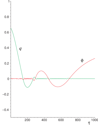
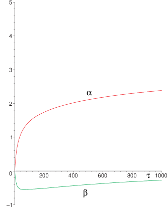
Figure 1: The scalars and logarithmic scale factors along a Kasner cosmological solution undergoing a conifold transition. The initial conditions are given in eq. (3.2).

The logarithmic scale factors thereby exhibit an initial period from $0\leq\tau\lesssim 200$, say, with a rapid increase of $\alpha(\tau)$ and decreasing $\beta(\tau)$. During this period the four-dimensional universe expands by a factor of five. After this initial period for large $\tau$ the both of the scale factors are almost constant.

The interesting feature of this solution is the dynamics of the scalar fields. For $\tau\lesssim 250$, say, the absolute value of $q(\tau)$ is large while the one for $\phi(\tau)$ is very small ($\xi\gg 1$), indicating that the solution evolves along the Higgs branch. For $250\lesssim\tau\lesssim 350$ we encounter a crossover, where $|q(\tau)|$ and $|\phi(\tau)|$ are comparable and the solution evolves in the central region. For $\tau\gtrsim 350$ the roles of $q(\tau)$ and $\phi(\tau)$ are reversed. Now $|q(\tau)|$ is small while $|\phi(\tau)|$ has become large $(\xi\ll 1)$. This indicates that the solution now evolves along the Coulomb branch, revealing that it has undergone a transition from one vacuum branch to the other.

We remark that a conifold transition requires non-vanishing initial values for $\phi$ or $\dot{\phi}$, and $q$ or $\dot{q}$ as both $\phi=\dot{\phi}=0$ and $q=\dot{q}=0$ are consistent solutions of the equations of motion. Solutions with initial conditions $\phi_{\rm init}=\dot{\phi}_{\rm init}=0$ always stay on the Higgs branch while those with $q_{\rm init}=\dot{q}_{\rm init}=0$ remain on the Coulomb branch. This implies that conifold transitions can only be described with an extended LEEA which explicitly includes all the massless states appearing at the conifold point, since otherwise we have $q_{\rm init}=\dot{q}_{\rm init}=0$ or $\phi_{\rm init}=\dot{\phi}_{\rm init}=0$ automatically.

Figure 2 shows the solution (3.2) projected onto the $\phi$-$q$-plane. The black lines, which close to the origin have the shape of a hyperbola, illustrate the equipotential lines of the scalar potential. They seem to converge at the points $(|\phi|=\sqrt{{\textstyle\frac{2}{3}}},q=0)$ and $(\phi=0,|q|=\sqrt{{\textstyle\frac{1}{2}}})$, but this is an artefact of our presentation, because these points are at infinite geodesic distance, as discussed in the previous section. The Coulomb and the Higgs branch are given by the vertical $q=0$ and the horizontal $\phi=0$ axes, respectively. The conifold transition corresponds to the solution ‘bending around the corner’ and going from one ‘valley’ to the other. From this picture it is also clear that one needs initial values where the scalar fields either start a little ‘uphill’, or have a non-vanishing velocity in the ‘uphill’ direction, in order to be able to cross from one branch to the other.

The other remarkable feature of figure 2 is that it shows the existence of an effective repulsive force which drives the scalar fields from the valleys to the central ‘stadium.’ Observe that the solution turns back twice from an excursion into a valley, even though its motion is roughly aligned to the flat direction. Also note that in its third move into a valley, which we interpret as a complete transition, it does not move as deeply into the Coulomb branch as it started in the Higgs branch. For the potential $\mathbbm{V}={\textstyle\frac{1}{2}}x^{2}y^{2}$ which is, up to the different prefactor, the leading term of the conifold potential (2.5), it was shown analytically in [22] that there is an effective potential for the motion along the valleys, which drives solutions towards the stadium. This is intuitively plausible, because away from the stadium the valleys become very narrow, resulting in a repulsive force acting on solutions which are not perfectly aligned to the flat directions. For the motion along the $x$-direction, say, the effective potential found in [22] is $\mathbbm{V}_{\rm eff}\propto\ln(x)$. In the conifold case there will be corrections, but the qualitative properties are the same. However, as we will discuss in the next section, this effective potential is only half of the story. The second effect, which strongly enhances the dynamical preference of solutions to stay in the stadium is the Hubble friction resulting from the coupling to gravity.

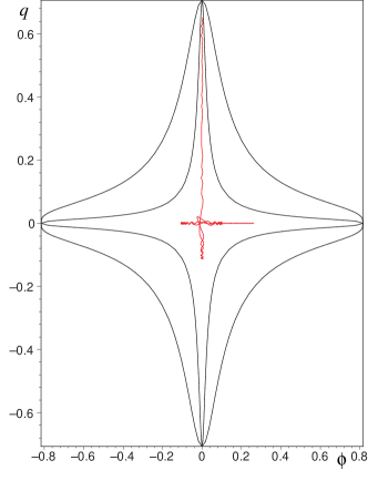
Figure 2: The cosmological solution (3.2) projected to the $q$-$\phi$-plane. The black lines are equipotential lines of the scalar potential. The four corners of the cross correspond to the boundaries of the scalar manifolds which are at infinite geodesic distance from the origin. The conifold transition reflects itself in the solution bending around the corner, switching from the Higgs to the Coulomb branch.

In our model generic solutions will ultimately be driven back to the stadium, an exception being those which are perfectly aligned to one of the flat directions as these run along their respective branch for infinite cosmological time. This is a limitation of our effective supergravity approach to topological phase transitions, which can only be overcome by lifting the discussion to the full string theory. Then the relevant scalar manifold does not just have two branches, but is the huge web (or ‘stratification’) composed of all the moduli spaces of Calabi-Yau spaces which can be connected by topological transitions. In fact, it is widely believed that the moduli space of all Calabi-Yau spaces form just one single connected web [23]. This web has many nodes, each of which corresponds to a (higher-dimensional version of a) stadium of the type considered in this paper. From this perspective, a plausible criterion for a completed transition between two branches is to require that a solution moves away from the stadium it has crossed by a distance which is larger than the distance to the next stadium. Clearly, the quantitative formulation and test of such a criterion would require to know the true metric on the web of moduli spaces. Since this is a formidable problem, we leave this challenge for future investigation and use the criterion introduced above.

Our numerical studies also yield some evidence that the motion of scalars in the conifold potential is chaotic since evolving two solutions with almost identical initial conditions may result in the two solutions evolving at two different vacuum branches at some later point in time. This is similar to observations made for the potential (2.6) which is also believed to exhibit chaotic behavior. Note that the valley structure of our potential provides one of the ingredients for chaos, namely a sequence of bifurcations. We, however, lack another typical ingredient, namely a hyperbolic fixed point of the equations of motion with both attractive and repulsive directions, so that the bifurcations lead to a stretching and folding of phase space volumes. As in flop transitions [12], the equations of motion have a family of non-hyperbolic fixed points, given by the vacuum manifolds $q=0$ or $\phi=0$, respectively. Therefore the standard methods of the theory of dynamical systems do not apply, and we fall short of a complete proof of chaotic behavior.

4 Moduli stabilization via Hubble friction

In the last section we noted that the dynamics of scalar fields showed a preference for the central region around the conifold point, or stadium. We now investigate this effect in detail. By comparing solutions with different, randomly chosen initial conditions we realize that for generic solutions the scalar fields get trapped in the stadium. Below we will give a representative example. In order to check to which extent the effect depends on the details of the potential, we present solutions for both the full conifold model (2.3), (2.4) and its leading order approximation (2.6) which (up to a constant factor) has been studied in [22, 8]. In order to compare the two cases we will transform the conifold model into the $(x,y)$-basis using eq. (2.5). We will also explore the role of Hubble friction by contrasting the numerical solutions of the full scalar equations of motion (2.11), (2.12) to solutions where the Hubble friction term proportional to $3\dot{\alpha}+\dot{\beta}$ has been switched off. All together we have the following four cases:
    i) leading order approximation without Hubble friction,
    ii) leading order approximation with Hubble friction,
    iii) conifold model without Hubble friction,
    iv) conifold model with Hubble friction.
In all cases we display solutions for the following initial conditions:

$$\begin{split}\phi(0)=&\,0.05\,,\quad\dot{\phi}(0)=0\,,\quad q(0)=0.6\,,\quad\dot{q}(0)=0\\ \Longrightarrow&\;\;x(0)=-0.061\,,\quad\dot{x}(0)=0\,,\quad y(0)=1.251\,,\quad\dot{y}(0)=0\,,\\ \quad\alpha(0)=&\,0\,,\quad\dot{\alpha}(0)=0.1\,,\quad\beta(0)=0\,.\end{split}$$ (4.1)

The initial value of $\dot{\beta}$ is again obtained from the condition that the initial values need to satisfy Friedmann’s equation.

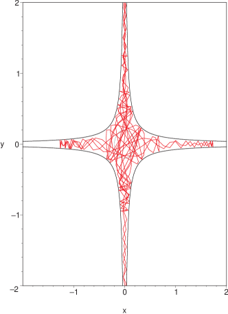
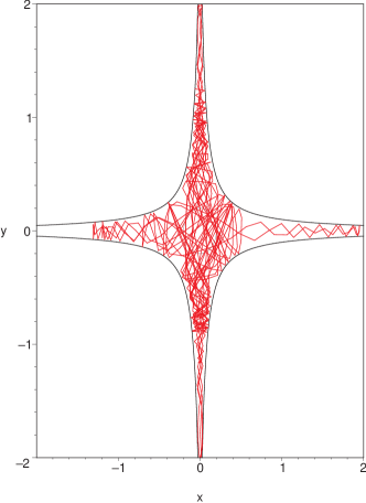
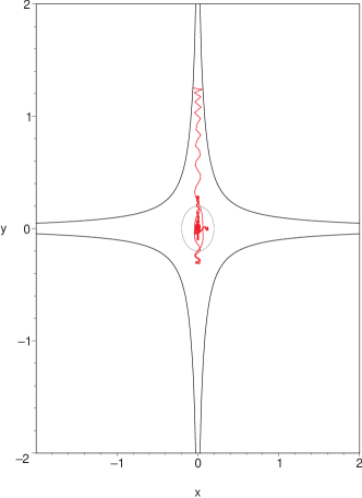
Figure 3: The solutions (4.1) arising from the setups i) (upper left), ii) (upper right), iii) (lower left), and iv) (lower right). The black hyperbolic lines are equipotential lines indicating the initial energy in the matter sector while the gray circle around the origin defines the stadium. Neglecting gravitational effects (left column) the solutions sample the allowed field space while including gravitational effects (right column) induces a trapping of the solution in the central region.

The resulting trajectories in the $(x,y)$-plane are shown in figure 3. Here the upper left, upper right, lower left and lower right diagram display the numerical solutions corresponding to case i), ii), iii), and iv), respectively. The hyperbolic black lines in these diagrams are the equipotential lines on which the solutions start with zero initial velocity. We have also added (in gray) a geodesic circle, which indicates the region we take to be the stadium.

Figure 3 immediately tells us two important messages. The first is that there is no difference in the qualitative behavior between the full conifold model and its leading order truncation. In both cases the potential (away from the bottom of the valley) has a gradient pointing in the direction of the central region. This gradient prevents the solutions from running off to infinity and turns them back to the stadium. The qualitative behavior of the solutions then depends on the presence of this property and is independent of the detailed shape of the potential.

The second message is that Hubble friction drastically changes the dynamics of the solution. If it is neglected, the scalar fields sample the region below the equipotential line on which they start. Although solutions never go very deeply into the valleys, and always return to the stadium after a while, they spend a considerable amount of time out in the valley. Thus there is a trapping of the moduli, but it is not very efficient. However, the picture changes drastically once Hubble friction is taken into account. Now we observe that the solutions just travel down the valley to the stadium and stabilize close to the conifold point.

This different behavior is easily understood in terms of the energy carried by the solutions. If Hubble friction is switched off in (2.11), (2.12) we have a geodesic motion modified by a force term, and the total energy $T+\mathbbm{V}$ is conserved. This is clearly visible in figure 3 where the solutions in the left column essentially sample the whole region which is energetically accessible. We say ‘essentially’ because the solutions never move very deeply into the valley although this is not forbidden by energy conservation. Once Hubble friction is included in (2.11), (2.12), the total energy $T+\mathbbm{V}$ of the scalar fields is no longer conserved. In an (overall) expanding universe, where $3\dot{\alpha}+\dot{\beta}>0$, $T+\mathbbm{V}$ decreases, and this damping leads to the immediate trapping of the solutions close to the conifold point. The fact that Hubble friction is very efficient in damping the motion of scalar fields in an expanding universe is of course well known. In principle, it can also happen that Hubble friction stops the motion of the moduli before such an ESP is reached [8]. The interesting point concerning our solutions is that (provided the initial values of $\dot{\alpha}$ and $\dot{\beta}$ are not chosen too large) they generically reach the stadium and get trapped at the conifold point. This effect is due to an interplay of two ingredients: the gradient of the scalar potential and Hubble friction. Without Hubble friction the trapping is inefficient, while Hubble friction alone only traps the solution at the bottom of the valley and not necessarily at the (physically interesting) ESP.

5 Discussion and Conclusions

In this paper we studied cosmological solutions of M-theory compactified on a Calabi-Yau threefold in the vicinity of a conifold singularity. The dynamics is described by a recently constructed low energy effective action [13, 14] which explicitly includes the M2-brane winding modes that become massless at the conifold point. Within this framework we found cosmological solutions which dynamically pass through the conifold transition. These solutions interpolate between Calabi-Yau compactifications with different massless field content and gauge group. Describing such dynamical transitions thereby requires that the dynamics of the winding modes is explicitly taken into account. While solutions which undergo topological transitions exist, they are suppressed while solutions which get trapped in the region of the conifold ESP are generic. Thus we see that the transition locus is dynamically preferred, even though the potential still has flat directions. In our case the moduli trapping occurs while supersymmetry is unbroken and the flat directions of the potential are not lifted.

The underlying effect is an interplay between the shape of the scalar potential and Hubble friction. The details of the potential are not relevant, in particular the full fledged supergravity model for a conifold transition and its non-supersymmetric first order approximation display the same type of behavior. This is similar to flop transitions where the scalar potential does not have a Higgs branch. Here, the non-supersymmetric truncations [17] and the full supergravity model [18] have the same qualitative dynamics. In both cases one observes perfect trapping, in the sense that the (numerical) solutions never left the transition region, despite that the potential had many flat directions. It remains, however, an open question to what extend the trapping depends on the number of flat directions. In this paper we have truncated the dynamics down to two scalars, corresponding to two one-dimensional branches, while in full string compactifications these branches are higher dimensional. Each additional flat direction opens a new opportunity for the scalar fields to escape the stadium and might weaken the trapping effect.

In [8] a different effect called quantum moduli trapping was discussed, which also works towards the stabilization of the moduli at ESPs. Here the trapping mechanism results from the quantum production of light particles in the vicinity of an ESP. This process extracts energy from the coherent motion of the scalar fields and converts it into particles. The feedback of the particle production on the scalar field induces an effective potential which drives the scalar field towards the ESP. The analysis of [8] focused on fast trapping, meaning trapping at time scales small compared to the Hubble time, $t\ll H^{-1}$. But it was also argued that quantum trapping also happens in an expanding universe. In this case Hubble friction plays an ambiguous role: it is potentially dangerous, because it can stop the scalar motion before an ESP is reached, but it is also needed to damp the oscillatory behavior of scalar fields induced by the quantum potential, so that the scalars really stabilize. Thus the mechanism is an interplay between a quantum effective potential (induced by particle production) with Hubble friction. A particularly interesting feature of quantum trapping is that inflation can arise as ‘trapped inflation’ [8].

In contrast, the potential featuring in our mechanism is ‘classical,’ in the sense that particle production is not taken into account. Since we include Hubble friction, we find that classical trapping is much more efficient than argued in the Appendix D of [8]. However, the classical trapping mechanism cannot produce inflation. In this respect the dynamics of the conifold potential is similar to the one of the flop model [18]: one can find short periods of accelerated expansion at collective turning points of the scalars, but the potential is either flat, but vanishing or non-vanishing, but too steep to sustain the accelerated expansion for an extended period of time. This situation might be ameliorated by switching on background fluxes to gently lift some of the flat directions.

Our conclusion is that both mechanisms, classical and quantum moduli trapping, are relevant and important for string cosmology. It would therefore be very interesting to include quantum trapping in the model studied in this paper. Other obvious extensions are the inclusion of flux, four-dimensional models or five-dimensional brane-world type models, and ESPs with non-Abelian gauge groups. This should give the answer to two important questions: (i) is the dynamics of string cosmologies such that they are generically attracted to interesting ESPs, and (ii) can one naturally have inflation ‘on the way’ to the ESP? Concerning point (i) it would be interesting to have an explicit realization of the ‘enhancement cascades’ mentioned in [8]. String moduli spaces have a hierarchy of special submanifolds with increasing numbers of symmetries and light particles for decreasing dimension of the ESP locus. One therefore expects that the moduli first move to an ESP hypersurface, and subsequently to subspaces of higher and higher Co-dimension. It would be interesting to see whether the resulting enhancement cascades have a high probability to end with a realistic particle spectrum, meaning a small standard model or GUT-like gauge group times a hidden sector.

References

- [1] P. S. Aspinwall, B. R. Greene, D. R. Morrison, Nucl. Phys. B 416 (1994) 543 [arXiv:hep-th/9309097].
- [2] B. R. Greene, D. R. Morrison, A. Strominger, Nucl. Phys. B 451 (1995) 109 [arXiv:hep-th/9504145].
- [3] E. Witten, Nucl. Phys. B 403 (1993) 159 [arXiv:hep-th/9301042].
- [4] E. Witten, Nucl. Phys. B 471 (1996) 195 [arXiv:hep-th/9603150].
- [5] B.R. Greene, String theory on Calabi-Yau manifolds, in Fields, strings and duality, Boulder (1996) 543, [arXiv:hep-th/9702155].
- [6] B. S. Acharya, S. Gukov, Phys. Rept. 392 (2004) 121 [arXiv:hep-th/0409191].
- [7] A. Strominger, Nucl. Phys. B 451 (1995) 96 [arXiv:hep-th/9504090].
- [8] L. Kofman, A. Linde, X. Liu, A. Maloney, L. McAllister, E. Silverstein, JHEP 05 (2004) 030 [arXiv:hep-th/0403001].
- [9] T. Mohaupt, Fortsch. Phys. 51 (2003) 787 [arXiv:hep-th/0212200].
- [10] T. Mohaupt, M. Zagermann, JHEP 12 (2001) 026 [arXiv:hep-th/0109055].
- [11] J. Louis, T. Mohaupt, M. Zagermann, JHEP 02 (2003) 053 [arXiv:hep-th/0301125].
- [12] L. Järv, T. Mohaupt, F. Saueressig, JHEP 12 (2003) 047 [arXiv:hep-th/0310173].
- [13] T. Mohaupt, F. Saueressig, Effective supergravity actions for conifold transitions, [arXiv:hep-th/0410272].
- [14] F. Saueressig, Topological phase transitions in Calabi-Yau compactifications of M-theory, Ph.D. Thesis, to appear in Fortschr. Phys.
- [15] I. Gaida, S. Mahapatra, T. Mohaupt, W. A. Sabra, Class. Quant. Grav. 16 (1999) 419 [arXiv:hep-th/9807014]
- [16] B.R. Greene, K. Schalm, G. Shiu, J. Math. Phys. 42 (2001) 3171 [arXiv:hep-th/0010207].
- [17] M. Brändle, A. Lukas, Phys. Rev. D 68 (2003) 024030 [arXiv:hep-th/0212263].
- [18] L. Järv, T. Mohaupt, F. Saueressig, JCAP 02 (2004) 012 [arXiv:hep-th/0310174]; ibid, in “Symmetries beyond the standard model”, Portoroz (2003) 254 [arXiv:hep-th/0311016].
- [19] G. Curio, A. Klemm, D. Lüst, S. Theisen, Nucl. Phys. B 609 (2001) 3 [arXiv:hep-th/0012213].
- [20] A. Giryavets, S. Kachru, P. K. Tripathy, JHEP 08 (2004) 002 [arXiv:hep-th/0404243].
- [21] T. R. Taylor, C. Vafa, Phys. Lett. B 474 (2000) 130 [arXiv:hep-th/9912152].
- [22] R. Helling, Beyond eikonal scattering in M(atrix)-theory, hep-th/0009134.
- [23] M. Reid, Math. Ann. 278 (1978) 329.