D-branes and BCFT in Hpp-wave backgrounds
Abstract:
In this paper we study two classes of symmetric D-branes in the Nappi-Witten gravitational wave, namely D2 and branes. We solve the sewing constraints and determine the bulk-boundary couplings and the boundary three-point couplings. For the D2 brane our solution gives the first explicit results for the structure constants of the twisted symmetric branes in a WZW model. We also compute the boundary four-point functions, providing examples of open string four-point amplitudes in a curved background. We finally discuss the annulus amplitudes, the relation with branes in and in and the analogy between the open string couplings in the model and the couplings for magnetized and intersecting branes.
CPHT RR 012.0304
KCL-MTH-04-15
LPTHE-04-28
1 Introduction
The study of gravitational waves as string theory backgrounds began more than fifteen years ago [1]-[7]. They were proposed as the most convenient starting point for extending the analysis of the properties of string theory from the familiar vacua given by the product of flat space and a compact manifold to the less explored curved, non-compact space-times. The main reason was that already from the point of view of general relativity the gravitational waves are some of the simplest time-dependent backgrounds. They admit a covariantly constant null Killing vector, most of their curvature invariants vanish and there is no particle creation. Another distinctive feature, which is particularly relevant for string theory, is that it is always possible to fix the light-cone gauge for the quantization of the world-sheet action. Recently it was also realized that the gravitational waves play an important role in the study of gauge/string duality.
Motivated by the notion of Penrose limits [8]-[9], it was argued [11] that such backgrounds are dual to modified large-N limits of gauge theories. This observation has opened new avenues in understanding stringy aspects of the gauge theory/string theory duality. Indeed, the Green-Schwarz action for the pp-wave that is obtained by the Penrose limit of , can be quantized in the light-cone gauge, even though there is a non trivial R-R flux [12, 13]. A lot of progress has been made since, and this is reviewed in [14]-[17]. It should be noted however that at the moment there is no generally accepted theory of the full holographic correspondence, although several proposals have been put forward [18]-[22].
Given the relevance for both the study of string theory in non-compact curved space-times and the gauge theory/string theory duality, we believe that it is important to obtain a clear and detailed understanding of the string dynamics at least in some particular gravitational wave backgrounds. With this aim in mind, it is natural that our choice falls upon a class of gravitational waves that are supported by a NS-NS flux and have an exact CFT description as WZW models. This is the class of the WZW models based on the Heisenberg groups , . The first example in this family was discovered by Nappi and Witten [7] and the others were introduced in [23],[24]. These models, unlike those with the same metric but supported by a R-R flux, can be quantized in a covariant way using standard perturbative string theory techniques. The presence of the affine symmetry algebra then imposes additional constraints that can lead to the complete solution of the model111See [25, 26] for a study of other interesting pp-waves without affine symmetry algebras.. Since the study of string and brane dynamics in non-compact curved backgrounds is a difficult arena, all models that can be solved exactly are a source of useful information. Unfortunately, only very few examples are available and they essentially amount to the Liouville model [27, 28, 29], to [30, 31] and its cosets [32]-[34].
In [35] we added another entry to this list, solving the model, which describes the propagation of a string in a four-dimensional gravitational wave. The structure of the closed string spectrum turned out to be very similar to the one established for [31]. It can be organized in highest-weight and spectral-flowed representations of the affine algebra and there are two distinct classes of states. For generic values of the light-cone momentum , the states belong to the discrete representations of the algebra. They correspond to short strings that are confined by the background fields in closed orbits in the plane transverse to the two light-cone coordinates. Whenever , with a parameter of the pp-wave metric, the states belong to the continuous representations of the algebra and correspond to long strings that move freely in the transverse plane.
In [35], we computed all the three and four-point correlation functions of primary vertex operators, thus providing all the structure constants for this non-compact WZW model. We also showed explicitly that the spectral-flowed representations are necessary for the consistency of the model since they appear in the intermediate channel of four-point amplitudes with external highest-weight states. In [36] we performed a similar analysis for the model. This model already displays all the new features of the higher-dimensional cases, namely the existence of enhanced symmetry points and the necessity of introducing representations that satisfy a modified highest-weight condition, which generalize the concept of spectral-flowed representations. The model is also relevant for the correspondence, being the Penrose limit of .
As conformal field theories, the model and its higher dimensional versions deserve attention not only because of the rich and interesting structure we have just outlined but also because there are several relations between them and other important models. Most of these relations follow directly from the original idea of Penrose of considering the gravitational waves as limits of other space-times. From the point of view of the world-sheet -model, the Penrose limit that connects two backgrounds both having an exact description as WZW models can be interpreted as a contraction of the underlying current algebra [37]. As such, the model captures the limiting behavior of backgrounds of the form and . In [35] we analyzed the contraction of to and in [36] the contraction of to .
The structure of the algebra changes drastically in the contraction process. The structure of the space-time is also drastically changing during the Penrose limit. Despite this, we have shown that it is possible to take the limit of the CFT operators and of the dynamical quantities such as the correlation functions in a controlled way. Another interesting relation stems from the free-field realization of the model introduced in [38, 39]. The primary vertex operators can be represented using the twist fields of the orbifold obtained as the quotient of the plane by a rotation and a dictionary can be established connecting the amplitudes computed in the model and the amplitudes computed in the orbifold CFT [35].
In this paper we complete our analysis of the model by studying D-branes in the Nappi-Witten gravitational wave and the dynamics of their open string excitations. The dynamics of open strings in curved space-time is even less understood than its closed counterpart and again we have at our disposal a very limited number of exactly solved examples. What is typically accessible, are the boundary states that have been studied for the Liouville branes [40, 41], for branes in [42, 43, 44] and for the 2d black hole [45, 46]. For all the other quantities such as the bulk-boundary and the three-point boundary couplings only partial results exist [44] and their computation proved to be an extremely difficult task. The only exception is the Liouville model for which the complete solution is available [40, 41, 47, 48, 49]. In this paper we will provide the complete solution for the BCFT pertaining to the two classes of symmetric branes of the model.
D-branes in pp-wave backgrounds have already been the object of several studies and we summarize here only the main results. D-branes in R-R supported pp-waves have been discussed in the light-cone gauge and various aspects of their physics have been analyzed [50]-[56]. Interesting world-volume theories have been argued to exist on such branes [57]. D-branes in NS-NS supported pp-wave have also been studied, since they are relevant for the Penrose limits of little string theory and, unlike the RR supported pp-waves, they are amenable to study using boundary CFT methods [58, 59],[60]-[63]. Our aim in this paper is not to describe the most general brane configuration in the Nappi-Witten gravitational wave. We focus instead on two particular classes of branes which preserve half of the background isometries and we clarify the closed and open string dynamics in full detail.
The model has two families of symmetric D-branes [58, 59], namely and branes. We solve in both cases the consistency BCFT conditions [75, 76] and obtain the BCFT data, that is, the bulk-boundary and the three-point boundary couplings. The bulk-boundary couplings for the branes can be found in Eq. and while the three-point boundary couplings are in Eq. , , and . The bulk-boundary couplings for the branes are in Eq. while the boundary three-point couplings can be found in Eq. and . To our knowledge, with the notable exception of the Liouville model [40, 41, 47, 48, 49], this is the first complete tree-level solution of D-brane dynamics in a curved non-compact background.
The D2 branes are the twisted symmetric branes of the model. Their world-volume covers the two light-cone directions and one direction in the transverse plane. The induced metric is that of a pp-wave in one dimension less and they also carry a null electromagnetic flux. As such, they provide an interesting example of curved branes in a curved space-time. The spectrum of open strings starting and ending on the same brane or stretched between different branes contains all the representations of the algebra.
There are many similarities between the D2 branes in and the branes in . This is not surprising since they can be considered as Penrose limits of specific branes in or in . More precisely, if we start from they arise from branes with Neumann boundary condition in time while if we start from they arise from the branes. The relation between the vertex operators and the orbifold twist fields leads in this case to an analogy between the D2 branes in the Nappi-Witten wave and configurations of intersecting branes in flat space [64].
The branes are the untwisted symmetric branes of the model. They have Dirichlet boundary conditions on the two light-cone coordinates and their world volume covers the transverse plane with an induced flat Euclidean metric. They are also supported by a world-volume electric field whose magnitude determines their localization in one of the light-cone coordinates. Having a non-trivial boundary condition along the real time direction they are examples of S-branes [65]. In fact, the Penrose limit relates the branes to either branes with a Dirichlet boundary condition in time in or to the branes in .
The world-volume of the branes shrinks to a point whenever their light-cone position is given by . For these values of the coordinate , there is another class of symmetric branes with a cylindrical world-volume. These branes extend along the light-cone direction and have a fixed radius in the transverse plane. We will not discuss them in detail in this paper. We also mention that the branes are a special case of a more general class of non-symmetric branes that we discuss from the DBI point of view. Finally, the behavior of the open strings attached to the branes is very similar to the behavior of open strings ending on magnetized branes in flat space [66].
Our solution of the model with boundary should be useful not only to improve our understanding of the closed and open string dynamics in curved space-times but also to clarify some properties of both compact and non-compact WZW models. Indeed, as it is widely appreciated by now, only when studied in the presence of a boundary a conformal field theory reveals its full richness. Among other results we provide the first example of structure constants for twisted symmetric branes in a WZW model (the D2 branes) and of open four-point functions in a curved background.
While the physical interpretation of the amplitudes in the presence of the branes is straightforward, the interpretation of the amplitudes for the branes is less evident, in particular when they involve open string states stretched between different S-branes which can be put on shell. They might play the role of boundary conditions at spatial infinity but at fixed time (specified by the S-brane in question). In fact thinking of an S-brane as a standard soliton supported by a scalar [65], we can imagine that they appear because of the special initial state of the scalars. In this context, the open string insertions can be interpreted as small variations on the initial data that “creates” the branes. It still remains to be seen whether such a setup may be realized in a problem with physical interest and whether the -branes can be relevant for cosmology.
In this paper, we also discuss the annulus amplitudes. Our results, even though suggestive, are not conclusive and the relation between the open and the closed string channel of the annulus certainly deserves further study.
The structure of this paper is the following: In section 2 we review the geometry of the symmetric branes of the WZW model, first considered in [58, 59]. We also discuss the relationship between branes in the Nappi-Witten gravitational wave and branes in and . In section 3 we evaluate the bulk-boundary couplings using the semi-classical wave functions. In section 4 we discuss the spectrum of the boundary operators. In section 5 we solve the Cardy-Lewellen constraints [75, 76] and display the structure constants of the boundary theory. In section 6 we discuss the four-point amplitudes. In section 7 we analyze the annulus amplitudes and discuss the contraction of the WZW model with boundary. In section 8 we analyze the physics of the branes in the Nappi-Witten gravitational wave using the Dirac-Born-Infeld action. Finally in section 9 we suggest some interesting lines of further research. Several technical details are collected in the appendices.
2 Branes in
The Nappi-Witten gravitational wave [7] is a curved homogeneous lorentzian space. The metric
| (2.1) |
solves the Einstein equations with a constant null stress-energy tensor, provided in our case by the 2-form field-strength
| (2.2) |
The light-cone and the radial coordinates are related to the cartesian ones by , and . As given before, the metric is in the so-called Brinkman form. The change of coordinates
| (2.3) |
gives the metric in Rosen form
| (2.4) |
In the following, both Brinkman and Rosen coordinates will be useful. The two-dimensional -model that describes the propagation of a string in this background is a WZW model based on the Heisenberg group [7]. The commutation relations are
| (2.5) |
where the generators and are anti-hermitian and . Even though the group is not semi-simple, there is a non-degenerate invariant symmetric form given by
| (2.6) |
which can be used to express the stress-energy tensor as a bilinear in the currents. For a detailed discussion of this model we refer the reader to [35].
Since this gravitational wave is a WZW model, we can study in considerable detail the symmetric branes, that is the branes that preserve a linear combination of the left and right affine algebras. The symmetric branes fall in families which are in one-to-one correspondence with the automorphisms of the current algebra. Given such an automorphism , the relevant boundary CFT is defined by the following boundary conditions on the affine currents
| (2.7) |
Equivalently we can introduce for each symmetric brane a boundary state that satisfies
| (2.8) |
The geometry of the symmetric branes in a group manifold has a simple and elegant description. Their world-volume coincides with the (twisted) conjugacy classes [67, 68]
| (2.9) |
where is the group automorphism induced by . A generic automorphism can be written as the composition of the adjoint action of a group element and of an outer automorphism
| (2.10) |
Since two families of branes that differ only in the choice of the inner automorphism are related by the left action of the group, we can set without loss of generality and restrict our attention to families of branes associated with distinct outer automorphisms . The algebra admits a non-trivial outer automorphism which acts on the currents as charge conjugation
| (2.11) |
As such, we have two families of symmetric branes, wrapped on the conjugacy classes and on the twisted conjugacy classes respectively. In the following, we will briefly review their geometry which was first discussed in [58, 59].
The conjugacy classes are characterized by two parameters, the constant value of the coordinate and the constant value of the invariant
| (2.12) |
Their geometric description is particularly simple in Rosen coordinates where the brane world-volume coincides with the wave-fronts since . These branes are thus Euclidean two-planes with an -dependent scale factor and a two-form field-strength
| (2.13) |
As usual, is the gauge invariant combination that appears in the Dirac-Born-Infeld action. These branes have a non-trivial boundary condition on the real time coordinate and can be called, following the modern terminology, -branes [65]. As we will show at the end of this section, they are related by the Penrose limit to the branes in or to the branes in with a Dirichlet boundary condition along the time direction.
The brane world-volume degenerates to a point whenever , . Indeed if we start from and change the value of until we reach , we interpolate between a point-like world-volume and a flat, infinite two-dimensional world-volume. This is very similar to what happens in flat space when we turn on a magnetic field on a brane and send its field-strength to infinity. As we will show in more detail later, there are several analogies between the untwisted symmetric branes of the model and branes in flat space with a magnetic field on the world-volume. In particular, the open strings stretched between two branes behave very similarly to the open strings in a magnetic field [66].
In Brinkman coordinates, the metric induced on the two-dimensional world-volume is trivial and the flux is
| (2.14) |
When we can parameterize the world-volume with and consider the brane as a point-like object which appears at the point and then moves away along the axis at the velocity of the light while simultaneously expanding in a circle in the transverse plane according to Eq. . When we have the time-reversed process, where an infinite circle coming from spatial infinity in the transverse plane shrinks to a point. Finally when the brane is a two-plane with a fixed light-cone position also in Brinkman coordinates.
When , the geometry of the conjugacy classes changes. In Rosen coordinates we notice that the two-dimensional planes degenerate to points. However, the transformation is singular when . Indeed, the analysis of the conjugacy classes shows that there are other possibilities for the symmetric branes at : when we have points with a fixed value of and when we have a cylinder of radius extended along the null direction . The geometry of the conjugacy classes is summarized in the following table
| branes | ||
|---|---|---|
| v, r = 0 | S(-1) branes | |
| r 0 | null branes |
In this paper we will often denote the two parameters that identify an branes with a single letter . It would be interesting to identify all these branes as bound states of some set of elementary branes. For instance, the branes in were shown to arise as bound states of branes [69]. In a similar spirit and with similar techniques we could choose as fundamental branes the point-like branes, that is the degenerate conjugacy classes for and try to identify the branes and the cylindrical branes as bound states of them.
The second class of symmetric branes we are interested in, wrap the twisted conjugacy classes which are parameterized by a single invariant
| (2.15) |
In Brinkman coordinates, they have a simple description as branes whose world-volume extends along the directions and is localized in the direction. They have a non-trivial induced metric, which describes a gravitational wave, and a null world-volume flux . The branes of the model thus provide an interesting example of curved branes in a curved space-time.
The Nappi-Witten gravitational wave is the Penrose limit of two simple and interesting space-times, and . For both space-times there is an exact CFT description in terms of WZW models based respectively on and , where the level is related to the radius of curvature. From the CFT point of view, the existence of the Penrose limit relating the Nappi-Witten wave and or corresponds to the fact that the current algebra is a contraction of the current algebras underlying the two original space-times [37].
We close this section by discussing the relation implied by the Penrose limit between the symmetric branes of the WZW model and the symmetric branes in and in . The latter branes have been studied in [67, 68, 70, 71]. In the first case, we will see that the branes arise from the branes in with a Dirichlet boundary condition in the time direction and that the branes arise from rotated branes in with a Neumann boundary condition in the time direction. In the second case, we will identify the branes as the limit of the branes in with a Neumann boundary condition in and the branes as the limit of the branes in with a Dirichlet boundary condition in . A similar discussion of the Penrose limit applied simultaneously to the space-time and to a brane contained in it can be found in [72].
We start with . Using the following standard parametrization for the group manifold
| (2.16) |
the metric and the two-form field-strength read
| (2.17) |
Along the time direction we can impose either Neumann or Dirichlet boundary conditions. As for the symmetric branes in , they wrap the conjugacy classes which are two-spheres characterized by a constant value of . Since does not have any external automorphism, the other possible symmetric branes are two-spheres shifted by the action of a group element and characterized by a constant value of . In order to take the Penrose limit we first perform the change of variables
| (2.18) |
and then send . In the limit
| (2.19) |
We observe that an brane with a Dirichlet boundary condition along the time direction becomes an brane labeled by the parameters and . Note that we have obtained the untwisted branes starting from branes whose world-volume does not contain the null geodesic used to define the Penrose limit. It is then natural to consider the limit of branes whose world-volume contains the null geodesic. For this purpose, we consider a family of branes rotated by and with a Neumann boundary condition along the time direction. In the limit, the parameter that characterizes the new family of branes behaves as follows
| (2.20) |
and they become the branes of the model. We can proceed in a similar way for the Penrose limit of and of its symmetric branes. We write the background in global coordinates
| (2.21) |
and define the Penrose limit introducing
| (2.22) |
and then sending to infinity. The conjugacy classes are characterized by a constant value of . In the limit
| (2.23) |
We observe that an untwisted symmetric brane of with a Dirichlet boundary condition in the factor gives rise to an brane in . Note that for large , the classes we are considering are precisely those with . This is precisely the branes and the degenerate branes in [71]. The null geodesic used in the limit is not contained in the brane world-volume. On the other hand, the twisted conjugacy class with a Neumann boundary condition in the factor, are characterized by a constant value of and contains the null geodesic. Since in the limit
| (2.24) |
we observe that the branes of the model are the Penrose limit of the branes.
A more detailed description of the Penrose limit for the different types of branes, using coordinate systems adapted to their world-volumes, can be found in Appendix E. In section 7 we will extend the analysis performed in [35] and discuss the contraction of the boundary WZW model which is the world-sheet analogue of the Penrose limit applied simultaneously to the space-time and to the brane contained in it.
3 Review of the bulk spectrum and semiclassical analysis
The structure of the Hilbert space of the WZW model [35] is very similar to the structure of the Hilbert space of the WZW model, clarified by Maldacena and Ooguri [31]. Together with the standard highest-weight representations of the affine algebra, restricted by a unitarity constraint, there are other representations that satisfy a modified highest-weight condition. These new representations are related to the standard ones by the operation of spectral flow, which is an automorphism of the current algebra. In our case there are three classes of highest-weight affine representations, reviewed in appendix A. To each affine representations we associate a primary chiral vertex operator
| (3.25) |
For the vertex operators, is the eigenvalue of and the highest (lowest) eigenvalue of . For the vertex operators, is related to the Casimir of the representation and is the fractional part of the eigenvalues of . Here is a coordinate on the world-sheet and a charge variable we introduced to keep track of the infinite number of components of the representations. On the charge variables the algebra is realized in terms of the operators
| (3.26) |
when considering its action on and by the operators
| (3.27) |
when considering its action on . States with with and fall into spectral-flowed discrete representations while states with with fall into spectral-flowed continuous representations . We also recall the relation
| (3.28) |
We will denote the image under spectral flow of a representation and the corresponding vertex operators either by , as we did before, or by the introduction of a further index . Finally the operator content of the bulk theory is given by the charge conjugation modular invariant. We then have the operators
| (3.29) |
as well as their images under an equal amount of spectral flow in the left and right sectors. The currents that generate the affine algebra preserved by the boundary conditions are given by the combination . A more detailed description of the representation theory of the affine algebra can be found for instance in [35].
Before performing the exact CFT analysis we will try to clarify the physics of the model in a semiclassical approximation. In doing so we will gain some intuition about the spectrum of the boundary operators and on the form of the bulk-boundary and the three-point boundary couplings. We use the following parametrization for the group elements
| (3.30) |
where . The isometry generators are and
To each vertex operator we can associate a semiclassical wave function. For the discrete representations they are
| (3.31) |
where , and , are two independent charge variables. The states that belong to these representations are confined in periodic orbits in the transverse plane, familiar from the quantum mechanical problem of a charged particle in a magnetic field. For the continuous representations we have
| (3.32) |
where , and , are two independent phases. The states that belong to the continuous representations can move freely in the transverse plane: the parameter is the modulus of the momentum and we can identify with its phase. These wave functions can be expanded in modes which represent the different components of the representations. It is also easy to compute semiclassical expressions for the bulk two and three-point functions.
We can proceed in a similar way for the states confined on the brane world-volume. In the case of the D2 branes, according to the boundary conditions (2.7), the generators of the unbroken background isometries are
| (3.33) |
They satisfy the commutation relation of the Heisenberg algebra and the brane spectrum, exactly as the bulk spectrum, can be organized in terms of representations. We then introduce three types of vertex operators for the open strings that live on a brane localized in the direction
| (3.34) | |||||
The operators that act on the charge variable are given by . The wave functions for the discrete representations are easily recognized as the generating functions for the Hermite polynomials. The open string states, as it was already the case for the closed string states, are trapped in periodic orbits in the direction of the brane world-volume unless their light-cone momentum is an integer. Note that for the boundary operators in the continuous representations can be an arbitrary real number.
Semiclassical expressions for the couplings between the bulk and the boundary operators can now be computed as overlap integrals of the corresponding wave functions on the brane world-volume. As a first example consider the bulk-boundary coupling . It is easily evaluated as
| (3.35) |
where
| (3.36) |
denotes a space-time integral restricted to the brane world-volume. The integral is non-zero only when and where . The other possible bulk-boundary coupling is given by
| (3.37) |
where . Since the D2 branes are invariant under translations along the two light-cone directions, only operators with and couple to their world-volume. Their one-point functions can be derived from the previous bulk-boundary coupling upon setting and integrating over
| (3.38) |
The discussion for the branes is very similar. The relevant isometry generators are and
| (3.39) |
They realize the algebra of the rigid motions of the plane and as a consequence the open string states that live on an brane labeled by can only belong to the continuous representations of the Heisenberg algebra. The semiclassical wave functions are
| (3.40) |
The action of the zero-modes of the currents on the charge variable is always given by . As we did for the branes we can now extract the bulk-boundary couplings from the overlap of the wave functions
| (3.41) | |||||
We see that all the discrete representations as well as the identity field have a non-vanishing one-point function, as expected since the branes brake the translational invariance in the light-cone directions. When the geometry of the conjugacy classes changes. The vertex operators have a non-vanishing one-point function only in the presence of the branes, localized at the origin of the transverse plane and at arbitrary positions in the light-cone directions
| (3.42) |
Translational invariance in the transverse plane being now broken, also all the continuous representations have a non-vanishing coupling
| (3.43) |
If we consider instead the cylindrical branes, extended along the direction and with a fixed radius in the transverse plane, only the vertex operators have a non-vanishing coupling
| (3.44) |
In the following we will not discuss in detail the cylindrical branes even though it would be interesting to extend our exact CFT analysis to them as well.
4 Spectrum of the boundary operators
In the previous section we discussed the semiclassical open string spectrum for the two families of symmetric branes we are studying in this paper. According to the semiclassical analysis, the states of open strings that live on a D2 brane, form all possible representations of the algebra. The states of open strings that live on an brane, can only belong to the continuous representations. In this section, we provide a detailed description of the spectrum of the open strings and extend the analysis also to the open strings that end on different branes. In close analogy with the bulk primary vertex operators, we introduce for each representation of the affine algebra, a boundary primary vertex operator , which depends on the insertion point on the real axis and on a charge variable . The two upper indices label the two branes on which the open string ends. This is the same as the two boundary conditions, the vertex operator interpolates between.
Let us start with a D2 brane localized at . The space of states contains in this case all possible representations of the algebra
| (4.45) |
This is very similar to what happens for the brane localized at in , where the spectrum is also given by the holomorphic square root of the bulk spectrum [73]. Similarly to that case, an observation about the spectral flow is in order [73]. Given a solution of the classical equation of motion, a new solution can be generated by the action of the spectral flow
| (4.46) |
where . Therefore
| (4.47) |
As we can see from , when only the spectral flow by an even integer is a symmetry of the D2 brane spectrum. Spectral flow by an odd integer maps a string living on a brane sitting at to a string stretched between a brane at and a brane at . As a consequence, we cannot use in the general case the spectral flow by an odd integer, to generate the complete brane spectrum, as we did in (4.45) for a brane sitting at the origin. However, using the relation , it is easy to verify that for the discrete representations, it is enough to consider the spectral flow by an even integer in order to obtain all possible values of the light-cone momentum. For instance, a state carrying a light-cone momentum , belongs to the representation .
For the continuous representations, the spectral flow by an even integer is not enough. We have to proceed in a different way [73]. We start with the vertex operator and take its image under the spectral flow by an odd integer . In this way, as explained before, we obtain the vertex operator pertaining to a string ending on the brane at and carrying an odd light-cone momentum. This asymmetry between the even and the odd spectral-flowed continuous representations will be also manifest in the annulus amplitude, as we will see in section 7. Summarizing, the spectrum of a brane localized at , is given by
| (4.48) |
The same structure of the spectrum holds for the strings ending on two different branes localized at and respectively. The only difference is that the possible values of the parameter that label the continuous representations are now constrained by . The minimal value of simply reflects the tension of the string stretched between the two branes. The fact that the bound depends on whether the amount of spectral flow is even or odd nicely reflects the different behavior of the continuous representations under the action of the spectral flow.
We now turn to the branes. As in the previous section, we use the short-hand notation for the boundary labels. The branes are Cardy branes. Therefore, a relation can be established between the parameters labeling the conjugacy classes and the quantum numbers of the representations
| (4.49) |
As usual, and . We will derive this relation in section 7, both by studying the annulus amplitudes of the model and by taking the Penrose limit of the WZW model. In close analogy with the D-branes in flat space, the quantum numbers and together with the spectral flow parameter , are related to the distance along the and the direction respectively. Using the relation (4.49), we can associate to a brane with labels the parameters , and . This is useful because as it is the case for the Cardy branes in a RCFT, the spectrum of open strings stretched from the brane to the brane is encoded in the fusion product of the two corresponding chiral vertex operators.
As mentioned earlier, the open strings ending on the same brane belong to the continuous representations of the algebra. The Hilbert space decomposes as
| (4.50) |
and the corresponding vertex operators are . The open strings that end on two different branes with labels and can belong to any of the highest-weight representations of the algebra as well as to their images under spectral flow. The precise representation depends on the distance between the two branes along the direction. We introduce the following notation: when we set , with and . We also define . The brane spectrum is then given by
| (4.51) |
and the vertex operators are . Similarly when we set with , . The brane spectrum is then given by
| (4.52) |
and the vertex operators are , . Finally when is an integer we set and we have
| (4.53) |
The vertex operators read . We assume that for our non-compact WZW model, the space decomposes as expected from the fusion rules. This assumption will be confirmed by the complete solution of the model that is presented in the next section.
For the branes, the spectral-flowed representations appear whenever the distance along the direction between two branes exceeds . In fact, the action of the spectral flow amounts to
| (4.54) |
that is
| (4.55) |
Note that in this case, the spectral flow is a symmetry for every integer and maps a string stretched between two branes localized at and to a string stretched from to . In the following, we will derive most of our results assuming that all the representations are highest-weight representations of the current algebra. It is however not difficult to extend our results to amplitudes involving spectral-flowed states, using the free-field realization [38, 39], as we did for the closed string amplitudes in [35].
5 Structure constants
A boundary conformal field theory is completely specified by three sets of structure constants: the couplings between three bulk or three boundary fields and the couplings between one bulk and one boundary field. These structure constants satisfy a set of factorization constraints first derived by Cardy and Lewellen [75, 76] (see also [77, 78, 79]). For the sake of clarity, we will briefly review the sewing constraints for a generic CFT and in the next section we will write them explicitly for the Nappi-Witten model.
For a CFT defined on the upper-half plane, there are two sets of fields. The first set contains the bulk fields , inserted in the interior of the upper-half plane and characterized by the quantum numbers . These quantum numbers specify the representations of the left and right chiral algebras. The second set contains the boundary fields , inserted on the boundary, (here the real axis). They are characterized by two boundary conditions and . They are also characterized by the quantum number , which labels the representations of the linear combination of the left and right affine algebras left unbroken by the boundary conditions. There are three sets of OPEs (we adopt with minor modifications the notation used in [78])
| (5.56) |
| (5.57) |
| (5.58) |
where . Here and in the following, the symbol will always denote the identity field and the one-point function of the identity with boundary condition on the real axis. Indexes are raised and lowered using
| (5.59) |
and for consistency we require that . Any correlation function on a Riemann surface with boundaries and with arbitrary insertions of bulk and boundary operators can be constructed by sewing together the basic amplitudes that correspond to the structure constants displayed in . The sewing constraints follow from the requirement that all possible ways of decomposing a given amplitude into the basic amplitudes lead to the same answer. The resulting constraints involve, besides the structure constants, the fusing matrices and the modular matrix. The fusing matrices , by definition, implement the duality transformations of the conformal blocks pertaining to the four-point amplitudes. Our conventions for the fusing matrices can be found in appendix B.
Sonoda [80] has analyzed the sewing constraints for Riemann surfaces without boundaries, and proved that the CFT correlation functions are unambiguously defined provided that the four-point functions on the sphere are crossing symmetric and that the one-point functions on the torus are modular covariant. Cardy and Lewellen extended these results to Riemann surfaces with boundaries [75, 76]. They proved that all the amplitudes are unambiguously defined provided that the structure constants satisfy four additional constraints. The first constraint is a quadratic constraint that follows from two different factorization limits of the bulk two-point function and reads
| (5.60) |
Here is the representation conjugate to , and represents the action of an external automorphism on the representations of the chiral algebra. A non-trivial has to be taken into account when considering for instance the symmetric branes of a WZW model. This constraint is a particular case of a more general one that follows from the factorization of a three-point function with two bulk and one boundary field.
The second constraint follows from two distinct factorization limits ( and respectively) of the four-point boundary correlator
| (5.61) |
and it reads
| (5.62) |
The third constraint, relates the bulk-boundary couplings and the boundary three-point couplings . It follows from the requirement of locality for a bulk field in a three-point function with two boundary fields
| (5.63) |
It can be written as follows
| (5.64) |
The fourth and last constraint involves the boundary one-point functions on the cylinder. When the boundary field is the identity, this constraint reduces to the Cardy constraint which relates the open and the closed string channel of the vacuum annulus amplitude. We postpone the analysis of this constraint to section 7.
In the following, we will determine the bulk-boundary couplings and the boundary three-point couplings for the two classes of symmetric branes of the WZW model. We will use as an input the structure constants and the fusing matrices of the model, as computed in [35]. Here, we only recall the two and the three-point couplings, while the fusing matrices are collected for convenience of the reader in appendix B. In order to write our formulae in a simple way, we shall leave in the following the dependence on the world-sheet variables and understood. We will write each bulk amplitude as the product of three terms, two kinematical parts and , which contain the dependence on the charge variables of the left and right chiral algebras, and a dynamical part . The form of and for the two and the three-point functions is completely fixed by the current algebra Ward identities222The factor for the three-point function, is the group-theoretic Clebsch-Gordan coefficient of the classical algebra .. Another convention we will commonly use is
| (5.65) |
for an -point amplitude with primary vertex operators carrying the labels . The non-trivial two-point functions are
| (5.66) | |||||
The bulk three-point couplings between three discrete representations are
| (5.67) | |||||
| (5.68) |
where . The corresponding kinematical factors are
| (5.69) |
with similar expressions for . The coupling between one continuous and two discrete representations is
| (5.70) |
where and we defined
| (5.71) |
We also have
| (5.72) |
Finally, the coupling between three vertex operators simply reflects the conservation of the momentum in the transverse plane. Therefore it is non-zero only when
| (5.73) |
It can be written as
| (5.74) |
where and .
We have now at our disposal all the information required to solve the WZW model with boundary. We will consider first the branes and use the sewing constraints to fix their structure constants. We will then study the branes that, as we already explained, are the Cardy branes of the model. In this case we compute the bulk-boundary couplings and verify that, for our non-compact WZW model, the boundary three-point couplings are also proportional to the fusing matrices. More details concerning the steps leading to the solution, can be found in appendix D.
5.1 The D2 branes
In this section we compute the structure constants for the maximally symmetric D2 branes of the Nappi-Witten model. From the physical point of view, the couplings we derive are important since they provide examples of open and closed string interactions in a non-compact, curved space-time. They are also interesting from a more formal point of view, since they represent the first example of the structure constants for the twisted symmetric branes of a WZW model. They could be a useful guide, leading to a general answer, extending the one that already exists for the Cardy branes. We will first derive the bulk-boundary couplings and then the boundary three-point couplings for strings ending on the same D2 brane at . Once these couplings are obtained, it is easy to generalize the solution to strings ending on different branes at arbitrary position in the direction.
The boundary two-point functions are
| (5.1.1) |
The second two-point function is non-zero only when . The bulk-boundary couplings have the following form
| (5.1.2) |
Here and the coupling is non-zero only when , . In order to write the couplings for the vertex operators, it is convenient to introduce two new angles defined by
| (5.1.3) |
We obtain
| (5.1.4) |
where and . The coupling with the identity can be obtained by setting and integrating over
| (5.1.5) |
There are two non-trivial bulk two-point functions that may be used to derive the constraint for the bulk-boundary couplings, namely and . The first one is very similar to the corresponding amplitude in flat space. Indeed, the form of turns out to be very simple
| (5.1.6) |
with and . The second correlator leads to the following constraint
| (5.1.7) | |||||
which is solved by
| (5.1.8) |
This exact result and the semiclassical computation (3.35) agree in the limit . Actually the two results differ only in that has to be replaced by in the argument of both the exponential and the Hermite polynomials and that the overall powers of have to become powers of . Note also the similarity of this coupling with the square-root of a bulk coupling of the form , as expected on general grounds. Finally, it is interesting to remark that the coupling vanishes when and it has to be replaced by the coupling with a spectral-flowed boundary operator. These couplings can be computed either using the free-field realization of [38, 39, 35] or by studying the factorization of a four-point amplitude with suitable external momenta.
We now proceed to the computation of the boundary three-point couplings. The D2 branes of the WZW model are not Cardy branes and in the absence of an one-to-one correspondence between the brane parameters and the representations of the chiral algebra, there is no natural relation between the boundary three-point couplings and the fusing matrices. In the absence of any ansatz, we have to solve directly the constraints. Fortunately, at least the couplings between open strings living on the brane at are simple. They are given by
| (5.1.9) | |||||
and we see that they are very similar to the square root of the bulk couplings. The kinematical parts can be easily obtained from and . The fact that the last coupling vanishes whenever is easy to understand if we perform a semiclassical computation using the wave functions (3).
In order to find the solution for branes sitting at arbitrary positions, we rely once more on the fact that the boundary vertex operators in the continuous representations are very similar to the standard tachyonic vertex operators in flat space. If we also take into account the finite length of the open string stretched between two branes at and , we conclude that the quantity that is conserved in the interactions of the vertex operators is not but
| (5.1.10) |
As a consequence, we expect that the general form of the coupling between three vertex operators in the continuous representations is
| (5.1.11) |
Consider now the correlator
| (5.1.12) |
where for clarity the numbers in the round brackets stand for both the charge variables and the worldsheet coordinates of the corresponding vertex operators. This correlator factorizes on a single block in the -channel and leads to the sewing constraint
| (5.1.13) |
where
| (5.1.14) |
Note that according to (5.1.11), when raising a continuous index we must multiply the coupling by . From the previous constraint, we may read the coupling between one continuous and two discrete representations
| (5.1.15) |
where . Actually, the phase proportional to is not fixed by equation but by the constraint associated with the correlator
| (5.1.16) |
which reads
| (5.1.17) |
In order to verify that the couplings in solve the previous constraint, one needs the integral . At this point the correlator
| (5.1.18) |
gives a constraint whose unknowns are the couplings between three discrete representations. The constraint is
| (5.1.19) |
and it involves the following fusing matrix
| (5.1.20) |
The integral on the right hand side can be evaluated using . We obtain
| (5.1.21) |
where
| (5.1.22) |
Similarly
| (5.1.23) |
where
| (5.1.24) |
The kinematical part is similar to the one given in . We did not check the constraint for this family of branes.
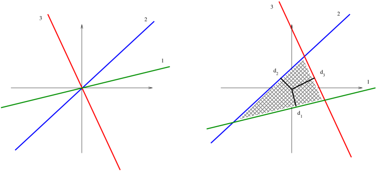
There are many similarities between the WZW model and the orbifold CFT of a plane with points identified by a rotation, stemming from the free field realization found in [38, 39]. It is therefore worth to compare the couplings derived in this section with the couplings for intersecting branes in toroidal compactifications, discussed in [87, 88, 89]. Actually, we can start directly from branes at angles in flat space. The boundary three-point couplings contains a quantum part that can be computed using orbifold twist fields [88, 89] and that coincides with and with . They also receive contributions from disc world-sheet instantons that behave as
| (5.1.25) |
where is the area of the triangle formed by the three intersecting branes (see fig. 1). Consider first three branes intersecting at the origin. In this case . The couplings in the model in this case contain no exponential contribution depending on the position of the branes. We now move each brane parallel to itself a distance from the origin. If we call the angle between the brane and the brane , the area of the triangle is
| (5.1.26) |
We recognize that the instanton contribution coincides with the exponential term in and upon setting and identifying the angles with the light-cone momentum carried by the vertex operators .
Finally there is an interesting limit to consider. The limit in the model is the analogue of the limit in which an brane is moved towards the boundary of . In this limit, as discussed in [73], one obtains a so called NCOS theory [82, 83], which is a theory of open strings decoupled from the closed string sector. In our case however there is an important difference: after the Penrose limit, the world-volume flux is null and therefore there is no notion of a critical electric field. In this respect, the world-volume theories of the branes provide examples of theories with light-like non-commutativity [84]. We may also observe that in the limit , only the bulk continuous representations remain coupled to the brane. The couplings in and between open strings in discrete representations are exponentially suppressed. Thus the strings interact in this limit only through the exchange of states in the continuous representations.
5.2 The branes
In this section we provide a detailed solution for the structure constants of the branes. We start with the boundary two-point functions for open strings ending on two different branes and , sitting at different positions in the direction. As explained in section 4, the vertex operators for the open strings stretched between the two branes belong to the representations, , when and to the representations, , when . We will use the shorthand notation where the sign in is fixed accordingly to the sign of . The two-point functions are
| (5.2.1) |
When the two branes are at the same position in the direction, the open strings ending on them belong to the continuous representations. In particular, when we have
| (5.2.2) |
The Ward identities completely fix the dependence of the bulk-boundary couplings on the charge variables
| (5.2.3) | |||||
The last coupling is non-zero only when and we set
| (5.2.4) |
The bulk one-point functions with the identity, are particular cases of the previous expressions
| (5.2.5) |
We can fix all the bulk-boundary structure constants by studying the factorization of the three kinds of bulk two-point functions, namely , (where we have to distinguish between and ) and . Using the bulk three-point couplings in and the fusing matrices in appendix B, the sewing constraints can be written as follows
| (5.2.6) | |||||
where and as before . The solution is
| (5.2.7) |
Note the similarity between the first coupling and a bulk three-point coupling of the form , as expected on general grounds. The second coupling can also be written as
| (5.2.8) |
Finally the one-point functions with the identity, relevant for the construction of the boundary states, are a particular case of the previous couplings and read
| (5.2.9) |
Whenever the couplings in simplify, since the brane is trivially embedded in the space-time. On the other hand, whenever , the behavior of the couplings in reflects the change in the geometry of the branes. We have first to multiply the structure constants by the one-point function of the identity . We then observe that the first coupling in becomes non-trivial only for , as expected since only these representations live on the brane world-volume. As for the couplings of the continuous representations, they are now non-zero for every value of while has to vanish. One can think of this process as an interpolation between Neumann and Dirichlet boundary conditions induced by the flux on the brane world-volume. In the limit these couplings reproduce the semi-classical expressions derived in section 3.
We determine now the boundary three-point couplings. Even though the explicit form of these couplings is slightly more involved than the couplings we computed in the previous section for the D2 branes, our task is in this case simplified since the branes are the Cardy branes of the WZW model. The three-point boundary couplings for Cardy boundary conditions in a RCFT, due to the one-to-one correspondence between the boundary labels and the representations of the chiral algebra, can be expressed using the fusing matrices. This was first realized in the case of the Virasoro minimal models [78]. Indeed, one can verify that setting
| (5.2.10) |
the constraint is satisfied as a consequence of the pentagon relation between the fusing matrices [85]. The previous relation proved very useful in order to study the effective field theory on the brane world-volume. Indeed, the fusing matrices of a WZW model based on the group coincide with the Racah coefficients of the quantum group algebra , where with the level and the dual Coxeter number. In the limit , the quantum Racah coefficients reduce to the classical ones, a fact that has been exploited in [69, 81] to study the non-commutative geometry on the brane world-volume. Similar observations were made also for some non-compact CFTs, most notably for the Euclidean version of [44] and the Liouville model [49]. We now verify that the relation between the fusing matrices and the three-point boundary couplings (5.2.10) remains valid also for the non-compact WZW model.
In the following, we will repeatedly use the relation between the brane parameters and the quantum numbers. As it was the case for the bulk theory, we can distinguish between various types of boundary three-point couplings. Consider three branes with labels , and . When , we have a boundary coupling similar to a bulk coupling
| (5.2.11) |
where . When , we have a boundary coupling similar to a bulk coupling
| (5.2.12) |
where . Finally, when we have a boundary coupling similar to a bulk coupling
| (5.2.13) |
with
| (5.2.14) |
The other configurations can be obtained by permuting the fields in the previous expressions. It is also useful to remember that for the continuous representations, raising an index is equivalent to while for the discrete representation it corresponds to .
We adopt now the following strategy. We assume that the three-point boundary couplings are given by the fusing matrices, up to a choice of normalization for the boundary fields. We then use the constraints pertaining to the correlators and to fix a convenient normalization for both the discrete and the continuous vertex operators. Finally we verify that the couplings determined in this way solve the other constraints as well.
Let us start with the three-point coupling between two open strings stretched between a pair of branes with labels and and an open string that lives on the world-volume of one of the two branes. This coupling involves two discrete and one continuous representation and is related to the following fusing matrix
| (5.2.15) |
with , and . Similarly,
| (5.2.16) |
with and . Here and are proportionality factors that can depend on all the quantum numbers involved even though we only emphasized their dependence on the labels and . The factorization constraint for reads
| (5.2.17) |
where and . Using the integral one can verify that the constraint is satisfied if the following relation holds between the proportionality factors
| (5.2.18) |
Combining the previous equation with the continuity of the two-point function on the disc
| (5.2.19) |
we obtain . A convenient choice for the normalization is
| (5.2.20) |
Once we make this choice, implies the following relation for the one-point function of the identity
| (5.2.21) |
which is satisfied if . This is indeed the case as we will se in section 7. We may now write
| (5.2.22) | |||||
with and a generalized Laguerre polynomial. Note the different behavior of the first of these couplings for and . In the first case it is non-zero only for and while it remains essentially unchanged in the second case. This is as expected since only the identity exists on the brane at while the open string spectrum for the brane at contains all the representations , .
Consider now the coupling between three open strings that live on the same brane. This is a coupling between three continuous representations. In terms of the fusing matrices we have
| (5.2.23) |
In this case we set which is equivalent to . The constraint for is
| (5.2.24) |
where , , and . In order to verify that this constraint is satisfied, one can use the series . The result is
| (5.2.25) |
with . For , the three-point function reproduces the two-point function in .
At this point, we have completely fixed the normalization of the boundary vertex operators. Thus, the factorization constraints for the other four-point amplitudes represent a consistency check on the solution.
The constraint for is slightly more complicated and reads
| (5.2.26) | |||
where , and . In order to verify that this constraint is satisfied one can use the integral . Consider now the couplings between states in discrete representations. Using the relation we can write
where , , and . Similar expressions hold for the other couplings between discrete representations and can be found in appendix D.
For completeness we display here the explicit form of one of these couplings
| (5.2.27) | |||||
where , , and
| (5.2.28) |
Note that . There are other constraints we should verify. We also checked the constraints following from amplitudes with one bulk and two boundary operators while we did not check the constraint related to the amplitude .
It is interesting to compare the coupling in (5.2.25) with the coupling between open tachyon vertex operators on a two-torus with a magnetic field [66, 86]. Consider two free bosonic fields and with the boundary conditions
| (5.2.29) |
where . In this case the momenta are measured using the open string metric
| (5.2.30) |
and the conformal dimension of a boundary tachyon vertex operator is
| (5.2.31) |
Moreover in the OPE there is a momentum dependent phase
| (5.2.32) |
where the deformation parameter is
| (5.2.33) |
Comparing the conformal dimension of with (5.2.31) we see that . Thus comparing the phase in (5.2.32) with the one in (5.2.25) we can identify
| (5.2.34) |
which is the expected result. Note that the magnetic field vanishes for , which corresponds to the flat brane or equivalently to Neumann boundary conditions on and . Changing the value of we get the mixed Neumann-Dirichlet boundary conditions in until we reach , where the field-strength diverges and therefore the boundary conditions become pure Dirichlet. In fact, precisely for these values of the coordinate , the two-dimensional conjugacy classes degenerate to points. According to the analogy with open strings in a magnetic field, the strings that live on the brane world-volume belong to the continuous representations since their ends are both subject to the same magnetic field and then they behave as free strings. On the other hand, the strings stretched between two different branes feel generically different magnetic fields and the corresponding vertex operators are therefore twist fields or, in terminology, they belong to the discrete representations. The twist for a string stretched from brane to brane is given by [66]
| (5.2.35) |
as expected. The effective field theory on the world-volume of an brane is the limit of the non-commutative field theory on the fuzzy sphere pertaining to the branes in : the volume and the magnetic flux are both scaled to infinity in order to obtain the non-commutative plane in the limit.
6 Four-point amplitudes
In the previous section we derived all the structure constants for the two families of boundary CFTs that describe the D2 and the branes of the WZW model. These are the essential ingredients for the solution of the models. We may now compute arbitrary correlation functions by sewing together the basic one, two and three-point amplitudes. Here, we are going to discuss in this section only those disc amplitudes that can be expressed in terms of the four-point conformal blocks, namely amplitudes containing either two bulk fields or one bulk and two boundary fields or four boundary fields .
In the following, we will provide some examples for each type of amplitude, both for the D2 and the branes. There are of course many other amplitudes one could consider, besides the few we are going to discuss here. In general, one can write for them a decomposition in terms of our conformal blocks and structure constants but we expect that using series and integrals more general than the ones we use in this paper one should be able to find a closed form for many of them. It will be interesting to analyze their properties in detail, both from the CFT and the string theory point of view.
As in the previous section, in order to avoid writing unnecessarily large formulae, we denote with a single number in round brackets all the variables a vertex operator depends on. This includes its insertion point and the charge variables. The four-point conformal blocks we will need in the following computations are displayed in appendix C. We choose the gauge
| (6.36) |
where , and the can represent the insertion points of either a bulk or a boundary vertex operator. Finally we set .
6.1 The D2 branes
For the branes we only display a very simple amplitude
| (6.1.1) |
In this case the integral over the conformal blocks can be performed explicitly and we obtain
where , and is a modified Bessel function. Moreover
| (6.1.3) |
Even though this amplitude does not depend on the brane parameters , it is interesting since we can expand it in powers of the charge variables and compare the correlator of the ground states of the representations with the correlator of open strings living at the intersection of two branes at an angle [88, 89], which can be described by boundary twist fields. The two expressions indeed coincide upon identifying the light-cone momentum with the angle formed by the two branes, as expected given the relationship between the primary vertex operators in the Nappi-Witten background and the orbifold twist fields [38, 39, 35]. Our open string amplitudes in the gravitational wave can be thought of as generating functions for the correlators of arbitrarily excited boundary twist fields in orbifold models or equivalently of open strings living at the intersection of a configuration of branes at angles.
6.2 The branes
For the branes we provide several explicit examples of four-point amplitudes. As we mentioned in the introduction, the space-time interpretation of these correlation functions deserves further investigation, in particular those involving on-shell open string states stretched between branes localized at different positions in the direction.
We start from the bulk two-point functions on the disc. This gives the first correction to the propagation of the closed strings due to the presence of the S-brane. Using the results of section 5 and the conformal blocks in appendix C we obtain
| (6.2.1) |
where are the brane parameters,
| (6.2.2) |
and
| (6.2.3) |
Here
| (6.2.4) |
When only the identity couples to the brane in the closed channel and the correlator simplifies
| (6.2.5) |
where
| (6.2.6) |
We also display the closely related amplitude
| (6.2.7) |
where
| (6.2.8) |
and
| (6.2.9) |
In this case
| (6.2.10) |
We consider finally
where and
| (6.2.12) |
We now turn to the four-point open string amplitudes. The cross ratio in this case is . The first amplitude we consider is
| (6.2.13) |
It describes the correlation between two open strings stretched between the branes and and two open strings ending on the brane . We obtain
| (6.2.14) |
where and
| (6.2.15) |
Moreover and
| (6.2.16) |
Another interesting amplitude is
| (6.2.17) |
which computes the correlation between four open strings stretched between the and the branes. When , we can use the integral and the result is
| (6.2.18) | |||
where
| (6.2.19) |
Moreover and
| (6.2.20) |
For the branes we showed that the boundary amplitudes can be considered as generating functions for the open string amplitudes in models with intersecting branes. In the case of the branes one can show in exactly the same way that the boundary amplitudes are generating functions for the open string amplitudes in models with magnetized branes. For instance, the amplitude between the ground states of the representations, which can be easily extracted from , coincides when with the amplitude computed in [90]. This result is not surprising since the magnetized and the intersecting branes in toroidal compactifications are related by the operation of charge conjugation, as it is also the case for the and the branes in the Nappi-Witten gravitational wave.
For the sake of completeness, we also present a correlator with one bulk and two boundary vertex operators. There are four types of such correlators
| (6.2.21) |
and the example we chose is
| (6.2.22) |
The cross-ratio in this case is and we have also defined
| (6.2.23) |
and
| (6.2.24) |
7 Annulus amplitudes
All the amplitudes we discussed so far, were defined on the disc. The consistency conditions of a boundary CFT impose a constraint also on the one-point functions of the boundary fields on the annulus. When the boundary field is the identity, this additional constraint reduces to the Cardy constraint, which interchanges the two equivalent interpretations of the annulus diagram. The first is the partition function of the boundary CFT, when time is running along the boundary. The other is as a tree-level amplitude for the propagation of the bulk states when time is running perpendicular to the boundary. In this second case the boundary conditions are specified by the introduction of two boundary states. Passing from one description to the other requires an S modular transformation , where is the modulus of the annulus.
The Cardy constraint has been at the origin of many important insights concerning the operator content of a rational boundary CFT [74, 77, 79]. It has also been exploited for the investigation of some non-compact models [42, 43, 44, 45, 46]. The best way to analyze the annulus constraint is to introduce characters for the representations of the chiral algebra and study their modular transformations. This is a non trivial problem for conformal -models describing non-compact curved space-times or time-dependent branes [45, 46, 91, 92, 93].
The characters of a generic representation of the affine algebra are defined as follows
| (7.25) |
For the representations we have
| (7.26) |
Note that , as required by (3.28). It is therefore convenient to express everything in terms of the characters, letting . It is useful to define
| (7.27) |
and rewrite the character as
| (7.28) |
We can derive the following S modular transformation
| (7.29) |
where
| (7.30) | |||||
The characters of the representations are
| (7.31) |
and they have the following modular transformation properties
| (7.32) |
where
| (7.33) |
Note that when = , all the representations with are inequivalent and their base is one-dimensional. The corresponding characters are
| (7.34) |
The torus vacuum amplitude of the Nappi-Witten gravitational wave [39, 94] can be expressed in terms of the characters. The discrete series contribution to the closed string partition function is given by
| (7.35) | |||||
Changing variable in each term of the sum and setting we obtain
| (7.36) |
where we performed the rotation in order to evaluate the gaussian integral. Similarly the contribution of the type-0 characters is
| (7.37) |
where is the volume of the transverse plane. This additional volume factor is a consequence of the fact that the states that belong to the continuous representations can move freely in the transverse plane and their wave functions are only delta function normalizable. On the other hand the discrete states are confined around the origin of the transverse plane and have normalizable wave functions.
We turn now to the annulus amplitudes. In the closed channel they can be constructed using suitable boundary states. In the open channel they encode the spectrum of the open strings ending on the two given branes. We will display the amplitudes in both channels and investigate how they are related by the modular transformation. In the following we will make several assumptions and formal manipulations and the results we obtain even though apparently consistent are not rigorous and we think that the modular properties of these amplitudes deserve further study. We will use the short-hand notation and . Boundary states for the WZW model 333Boundary states for the WZW model were also considered in the recent paper [95]. can be easily constructed using the bulk-boundary couplings derived in section 5. The boundary state for a D2 brane localized at is
| (7.38) | |||||
Here we have a factor of , since the boundary continuous representations correspond to one-dimensional waves. The annulus amplitude in the closed string channel for two branes localized at and then reads
| (7.39) | |||||
On the other hand, since the spectrum of the BCFT contains all the representations, the annulus amplitude in the open channel reads
| (7.41) |
where . We introduced the quantity in order to specify the domain of the integral in . The contribution of the continuous representation can also be written as
| (7.42) |
Note that the even and odd spectral-flowed continuous representations appear with different ranges of integration in the partition function, a remnant after the Penrose limit of the different density of the corresponding states for the branes in [73].
If we compute the modular transformation of the transverse annulus using the matrix in , we correctly reproduce the spectrum of the continuous representations in the direct annulus. It is less clear how the discrete contribution should appear. By comparing the normalization of the annulus amplitude in the direct and in transverse channel we can fix the one-point function of the identity. We have
| (7.43) |
The discussion for the branes is similar. The boundary state for an brane labeled by is
| (7.44) |
The bulk-boundary couplings with the identity are
| (7.45) |
and we recall the relations and . The annulus amplitude in the closed channel reads
| (7.46) | |||||
where we used the fact that also for the continuous representations when . In the previous expression we separated the contribution of the discrete and the continuous representations, which are weighted by different volume factors. In fact the first term has to be considered as a regularized term without the divergences due to the almost delocalized states in the transverse plane with , and the second term as the term containing all these divergences, since the continuous representations capture the behavior of the discrete representations when approaches an integer value. What this means is that when manipulating the term containing the discrete representations, whenever a constraint arises forcing to evaluate it at the boundary of the interval , the corresponding contribution should be discarded and only the contribution coming from the continuous representations in the second term of (7.46) retained. Equivalently, we could keep only the first term in and take into account the divergent behavior of the integrand when becomes an integer. We will show in the following that both points of view lead to the same result.
Let us transform the amplitude to the open string channel using the matrix in , writing for instance
| (7.47) |
We perform first the integration over which gives the constraint
| (7.48) |
Let us suppose for the moment that so that only the discrete representations contribute. We can recombine the integral over and the sum over in a single integral over
| (7.49) |
We now need a prescription to perform the integral over . The prescription that reproduces in the open channel the spectrum of the boundary operators is the following
| (7.50) |
Consider for instance the case even. We can expand
| (7.51) |
and then perform the integral over that gives the constraint
| (7.52) |
Therefore
| (7.53) |
This is precisely the expected result for the annulus amplitude in the open string channel. The reason is that when with and , the open string spectrum only contains discrete spectral-flowed representations
| (7.54) |
From the comparison of the amplitudes in the open and closed string channel, we can fix the last structure constants required for the complete solution of the boundary model, namely the one-point functions of the identity. We obtain
| (7.55) |
When with , the constraint has two solutions, , and , . We have two options. The first is to think as proposed before, that the term that contains the discrete representations is a regularized term. In this case, it does not contribute while the term containing the continuous representations after the modular transformation gives
| (7.56) |
This is the expected result, since whenever and the open string states belong to the continuous spectral-flowed representations
| (7.57) |
The second option is to think of the continuous representations as already included in the divergent behavior of the discrete representations for close to an integer. It is instructive to derive once more, adopting this point of view, and to show explicitly its equivalence with the previous one. In this case, we have to extract from the integral over the discrete representations when the integrand is evaluated at the extrema of the interval. Performing the same steps as before and keeping both contributions , and , , we obtain
| (7.58) |
Using the explicit form of the characters and sending , the previous expression can be rewritten as follows for
| (7.59) |
We should now interpret the divergence as due to the infinite volume of the transverse plane (consistently with the power we have of the modular parameter which is the one commonly associated with two non-compact directions)
| (7.60) |
which is the volume measured using the open string metric [86]
| (7.61) |
In this way, we obtain again the amplitude displayed in .
As we mentioned earlier, our aim in this section is not to provide a rigorous discussion of the modular transformation properties of the annulus amplitudes, but rather to give a plausible suggestion about how the standard open-closed duality should work for the branes of the model.
7.1 Contraction of the BCFT
The Penrose limit that connects the Nappi-Witten gravitational wave and or can also be extended to the branes contained in these space-times, as described in section 2. In [35] we gave a detailed description of the world-sheet equivalent of the Penrose limit in space-time. This is the contraction of the WZW model to the WZW model. It is interesting to perform the same contraction for the boundary CFT. Here we shall comment on how the BCFT describing the branes arises as the limit of the BCFT describing the branes in . We first recall how to derive the affine characters from the contraction of the characters [35]. It is convenient to write the latter as follows
| (7.1.1) |
where is the spin of the representations and
| (7.1.2) |
The characters are
| (7.1.3) |
The characters of the original CFT become the characters if we send the level to infinity and scale simultaneously the spin and the charge in a correlated way
| (7.1.4) |
More precisely for the discrete representations we obtain
| (7.1.5) |
with . The characters for the continuous representations require a different scaling, namely
| (7.1.6) | |||||
In the following, we will only discuss the contraction involving the WZW model. Similar relations however, can be written for the characters. The boundary state for an brane in reads
| (7.1.7) |
Here, we are considering the general case where the gluing condition (2.7) also involves the adjoint action of a group element . The are the matrix elements of in the spin representation and can be expressed in terms of the Jacobi polynomials
| (7.1.8) |
Finally is the modular S matrix of the affine algebra
| (7.1.9) |
Using the fact that for the label of the branes is related to the coordinate by
| (7.1.10) |
we can derive the relation between the brane parameters and the quantum numbers of the representations that is inherited from the original relations between the brane parameters and the spin of . The results are summarized in the following table. In the first column we listed the discrete representations. In the second and in the third column we show the labels of the corresponding branes. Finally, in the fourth column, we list the representations they originate from in the Penrose limit
In a similar fashion, one may show that the label of the branes is related to the label of the original brane by
| (7.1.11) |
We may now write down the annulus amplitudes for the brane configurations in whose Penrose limit is one of the branes in , as explained in section 2. We will show that in the limit, the direct and the transverse annulus amplitudes become the corresponding amplitudes for the model we discussed in the previous section. In order to do this, we have to first understand for each amplitude, how we can scale the quantum numbers of the original representations and then restrict our attention to states that have finite charges and conformal dimension in the limit.
For the D2 branes, we start with a brane with Neumann boundary conditions along the time direction. The original annulus amplitude in the open string channel is
| (7.1.12) |
The brane labels have to be scaled in the limit as , and therefore the range of the possible representations is
| (7.1.13) |
Since there is a lower bound in the range of , we have to slightly change the way we scale the spin in the Penrose limit. For the representations we simply set
| (7.1.14) |
and similarly for all the other discrete representations. For the continuous representations, the lower bound in shifts the lower bound for the integral in . It is easy to se that
| (7.1.15) |
We observe that the different behavior of the even and odd spectral-flowed continuous representations, arises also in a very transparent way from the contraction of . Note that the minimal conformal dimension for the vertex operators is , which can be ascribed to the tension of the string stretched between the two branes, as expected. Since the original amplitude contains arbitrary charges, in the limit we obtain an amplitude that contains all possible representations
| (7.1.16) |
In the transverse channel we can reason in the same way. The original amplitude is
| (7.1.17) |
Since now all the states have zero charge, according to (7.1.5-7.1.6) we can only obtain in the limit the highest-weight continuous representations.
The discussion for the branes is similar. We label the branes with their position in time and with the spin . In the open string channel, the original amplitude is
| (7.1.18) |
We scale , . As before we have to distinguish two cases. When is not an integer multiple of , we may write
| (7.1.19) |
with . We then have to scale as and the possible values of follow from the original range of
| (7.1.20) |
in integer steps and therefore , , as expected. On the other hand, when , we may use the relations . In the limit, we obtain an annulus amplitude that only involves the continuous representations.
In the closed string channel, the original amplitude is
| (7.1.21) |
As in the amplitude (7.1.12), we have again arbitrary charges. We thus obtain in the limit all possible representations. Therefore, the annulus amplitudes, both in the closed and in the open string channel, reproduce in the limit the results we expect for the and the branes. It would be very interesting to pursue this line of thinking, in order to gain a more detailed understanding of the contraction of the boundary CFT.
8 The DBI approach
We will study here the DBI approach for the branes described in this paper. This approach although in most cases approximate, has the advantage of an obvious geometric interpretation. We will also be able to provide an independent confirmation of the spectrum of fluctuations for the branes and justify some of the assumptions made during the solution of the BCFT. In the bosonic case the lowest state is the tachyon. In anticipation of the supersymmetric case we will use the bosonic part of the supersymmetric DBI action that describes the dynamics of the “massless” modes. To simplify the formulae, we use here the background (2.1,2.2) with so that the metric and antisymmetric tensor read
| (8.22) |
We can put back by rescaling , .
8.1 The branes and the spectrum of their fluctuations
We will find a class of solutions to the DBI equations that will contain as special cases the branes discussed in this paper. The will have Dirichlet boundary conditions on the coordinates. We choose a static gauge where the brane world-volume is parameterized by . The induced metric and antisymmetric tensor is
| (8.1.1) |
| (8.1.2) |
In the formulae above, a dot stands for a derivative and a prime for an derivative.
We can directly evaluate the Nambu-Goto-Dirac-Born-Infeld Lagrangian as
| (8.1.3) |
where is the world-volume gauge field strength. The equations of motion for the gauge field can be integrated to
| (8.1.4) |
where E is a constant (the “electric field”). The equations are
| (8.1.5) |
| (8.1.6) |
We will from now on consider a rotationally invariant ansatz. Dropping -derivatives the equations simplify to
| (8.1.7) |
with integration constants and from (8.1.3) given by
| (8.1.8) |
Massaging (8.1.7,8.1.8) we obtain
| (8.1.9) |
| (8.1.10) |
We will look here for solutions where is a constant corresponding to the symmetric branes discussed in this paper. constant implies that and
| (8.1.11) |
Since the class variable is , we learn that the symmetric branes have also . Comparison with (2.12) and (2.14) gives
| (8.1.12) |
The fluctuations around the classical embedding are in one-to-one correspondence with on-shell open marginal deformations. Although for a single brane this is not very rich, it is still useful to verify it explicitly. The richer case of two branes at a non-zero distance in light-cone is much harder to analyse and we will not do it here.
In appendix (F) we analyse the action for the fluctuations around the S1 solution that turns out to be
| (8.1.13) |
The equations of motion that ensue are
| (8.1.14) |
| (8.1.15) |
with the gauge field satisfying
| (8.1.16) |
with a constant.
The regular solution of (8.1.14) is constant. On the other hand, the solution of (8.1.15) is
| (8.1.17) |
In order to be regular at , the electric field fluctuation and the fluctuation must be related by
| (8.1.18) |
This is indeed implied by (8.1.12). In the non-symmetric case where (8.1.12) is no longer valid, (8.1.18) must still be in effect for the fluctuations to be continuum normalizable and thus physical states of the theory.
The two physical states obtained correspond to and in the bosonic case and and in the supersymmetric case [96] in accordance with the BCFT discussion. Note that here, unlike the D-brane case, including the contribution of the additional coordinates of the ten-dimensional string theory does not change our results. The reason is that the world-sheet is Euclidean and the physical states conditions are very restrictive, implying the vanishing of all momenta.
8.2 The D2 branes and the spectrum of their fluctuations
The cartesian coordinates on the plane are more convenient here. The metric and antisymmetric tensor read
| (8.2.1) |
Putting Dirichlet boundary conditions on we obtain the following induced metric
| (8.2.2) |
while
| (8.2.3) |
The action is
| (8.2.4) |
with
| (8.2.5) |
We will now search for solutions where the D2 brane is sitting at constant that contain the symmetric D2 solutions studied in this paper.
Setting we obtain the following equations to be solved
| (8.2.6) |
| (8.2.7) |
| (8.2.8) |
with
| (8.2.9) |
while the y equation gives444There is another possibility here, namely , but this does not correspond to a symmetric solution.
| (8.2.10) |
Equations (8.2.6-8.2.8) are then solved by
| (8.2.11) |
The symmetric solution corresponds to . The gauge field can be dualized to a scalar here as follows
| (8.2.12) |
Solving for the gauge field strength we obtain
| (8.2.13) |
Such expressions solve equations (8.2.6)-(8.2.7) but now the Bianchi identity gives
| (8.2.14) |
where
| (8.2.15) |
Using (8.2.10), (8.2.14) becomes
| (8.2.16) |
Thus the corresponding to our previous solution is
| (8.2.17) |
We will now study the spectrum of fluctuations around the simplest solution , , . Setting , , , and expanding the action to quadratic order we obtain
| (8.2.18) |
The ensuing equations of motion are
| (8.2.19) |
| (8.2.20) |
| (8.2.21) |
| (8.2.22) |
Introducing a dual scalar field A by
| (8.2.23) |
the equations read
| (8.2.24) |
where
| (8.2.25) |
In terms of the dual variable, the quadratic action can be written as
| (8.2.26) |
Defining a new complex scalar field as we find
| (8.2.27) |
Thus, is a massless scalar. Its solutions are in one-to-one correspondence with the discrete and the continuous representations in accordance with the BCFT discussion.
Since here the world-volume has Minkowski signature it is the eigenvalues of the Laplacians that are relevant when we include 6 extra flat coordinates in order to study strung theory in the background. Thus we need to solve
| (8.2.28) |
We parameterize,
| (8.2.29) |
and satisfies the harmonic oscillator equation
| (8.2.30) |
with quantized values of . For the equation becomes
| (8.2.31) |
and the solutions for are plane waves in one dimension.
Thus, the spectrum is in agreement with the BCFT findings in section 4.
9 Conclusions and generalizations
In this paper we provided the complete solution for the BCFT pertaining to the two classes of symmetric branes of the model, the and the branes. In both cases we solved the consistency BCFT conditions [75, 76] and obtained the BCFT data, namely the bulk-boundary and the three-point boundary couplings.
The bulk-boundary couplings for the branes can be found in Eq. and while the three-point boundary couplings are in Eq. , , and . The bulk-boundary couplings for the branes are in Eq. while the boundary three-point couplings can be found in Eq. and . To our knowledge, with the notable exception of the Liouville model [40, 41, 47, 48, 49], this is the first complete tree-level solution of D-brane dynamics in a curved non-compact background.
Our solution of the model with and without a boundary should help to clarify the properties of the non-compact WZW models and the closed and open string dynamics in curved space-times. Among other results we provided the first example of structure constants for twisted symmetric branes in a WZW model (the D2 branes) and of open four-point functions in a curved background.
There are two aspects of our work we think deserve further study. The first is to perform a more detailed analysis of the four-point amplitudes and the second to clarify the relation between the open and closed string channel of the annulus amplitudes. There are also several other issues it would be worth pursuing and we mention here a few. One is the study of the symmetric branes of the other WZW models based on the Heisenberg groups , . Their generators satisfy the following commutation relations
| (9.32) |
with . It will be interesting to generalize our results to the higher dimensional analogues of the and the branes as well as to extend them to encompass other classes of symmetric branes. In fact whenever two or more of the parameters in (9.32) coincide, the higher dimensional Heisenberg algebras have additional outer automorphisms which permute the corresponding pairs of generators. The existence of additional outer automorphisms parallels the enhancement of the isometry group of these pp-wave backgrounds when some of the parameters coincide [36]. As a consequence these models display a richer set of symmetric branes, some of them similar to the oblique branes discussed in [54, 52, 72].
It should also be possible to study less symmetric branes which can be obtained by performing a -duality along the Cartan torus, following [97]. Also the supersymmetric WZW models should be analyzed and brane configurations preserving some or none of the bulk supersymmetries. An interesting brane is the brane in the gravitational wave [58, 59], the Penrose limit of the brane in . The dynamics of the open strings ending on this brane should be described by a direct generalization of our results for the branes.
10 Acknowledgments
The authors are grateful to Costas Bachas and Volker Schomerus for several discussions. G.D. would like to thank the Erwin Schrödinger International Institute in Vienna for the warm hospitality provided to him during the program String theory in curved backgrounds and BCFT and the workshop String theory on non-compact and time-dependent backgrounds, June - . He is particularly grateful to the organizers of the program for the brilliant atmosphere they created and for giving him the opportunity to present this work. Most of the present work was done while G. D. was supported by an European Commission Marie Curie Individual Postdoctoral Fellowship at the LPTHE, Paris, contract HMPF CT 2002-01908. G.D. also acknowledge support by the PPARC grant PPA/G/O/2002/00475 and by the EU network HPRN-CT-2000-00122. The work of E. K. was partially supported by INTAS grant, 03-51-6346, RTN contracts MRTN-CT-2004-005104 and MRTN-CT-2004-503369 and by a European Union Excellence Grant, MEXT-CT-2003-509661.
Appendices
Appendix A representations
The Heisenberg group has three types of unitary representations.
1) Lowest-weight representations , where . They are constructed starting from a state which satisfies , and . The spectrum of is given by , and the value of the Casimir is .
2) Highest-weight representations , where . They are constructed starting from a state which satisfies , and . The spectrum of is given by , and the value of the Casimir is . The representation is the representation conjugate to .
3) Continuous representations with . These representations are characterized by , and . The spectrum of is then given by , with and . The value of the Casimir is . The one dimensional representation can be considered as a particular continuous representation, where the charges and are zero.
For the study of the WZW model, three types of highest-weight representations of the affine algebra will be relevant. Affine representations based on representations of the horizontal algebra, with conformal dimension
| (A.33) |
and affine representations based on representations, with conformal dimension
| (A.34) |
Highest-weight representations of the current algebra lead to a string spectrum free from negative norm states only if they satisfy the constraint
| (A.35) |
States with larger values of belong to new representations resulting from spectral flow of the original highest-weight representations [31, 38]. In fact the spectral-flowed representations are highest-weight representations of an isomorphic algebra whose modes are related to the original ones by
| (A.36) |
An important piece of information for understanding the structure of the three-point couplings is provided by the decomposition of the tensor products of the representations
| (A.37) |
The fusion rules for the primary vertex operators of the model can be obtained from the previous tensor products. When the representations involved are spectral-flowed representations, one has to use the relation [98]
| (A.38) |
Appendix B Fusing matrices
Consider the correlator and let denote the conformal blocks in the -channel and the conformal blocks in the -channel , where . We use the following convention for the fusing matrices
| (B.39) |
defines a linear transformation
| (B.40) |
where is the space of the three-point couplings. Moreover,
| (B.41) |
Since in our non-compact CFT the conformal blocks are labeled either by discrete or continuous indexes, in the previous expressions we will have a sum or an integral, according to the case. The following are the fusing matrices we used in section 5 to compute the structure constants. We set . For correlators of the form we have
| (B.42) |
where
| (B.43) |
For correlators of the form we have
| (B.44) |
where
| (B.45) |
| (B.46) |
| (B.47) |
| (B.48) |
Similar expressions hold for correlators of the form .
| (B.49) |
where
| (B.50) |
| (B.51) | |||
| (B.52) | |||
For correlators of the form we have
| (B.53) |
| (B.54) |
where , and .
Appendix C Bases of conformal blocks
In this appendix we collect various bases of conformal blocks for correlators of the form , and . Using the global conformal and symmetries, the four-point amplitudes can be written as follows
| (C.55) |
The kinematical functions and are completely fixed by the Ward identities of the left and right algebras and we chose the standard gauge for the global conformal transformations. The conformal blocks thus depend only on the cross-ratio and a suitable combination of the four charge variables. In the following . Consider first the correlator
| (C.56) |
The Ward identities require
| (C.57) |
and give the function
| (C.58) |
as well as the invariant combination
| (C.59) |
We set where
| (C.60) |
We then arrive at the following form for the KZ equation
| (C.61) | |||||
The correlator vanishes when . In the -channel we have the representations with . The conformal blocks are
| (C.62) |
where
| (C.63) |
and
| (C.64) |
In the -channel we have the representations , and their conformal blocks read
| (C.65) |
where
| (C.66) |
and
| (C.67) |
Consider now the correlator
| (C.68) |
The Ward identities require
| (C.69) |
and give the function
| (C.70) |
In this case the invariant combination is
| (C.71) |
We set where
| (C.72) |
We then arrive at the following form for the KZ equation
| (C.73) | |||||
When in the -channel we have with for and with for . The conformal blocks are
| (C.74) |
where is the n-th generalized Laguerre polynomial,
| (C.75) |
and
| (C.76) |
When , the intermediate states belong to the representation with with for and for . The conformal blocks are very similar. Finally when and the intermediate representation is and the conformal blocks read
| (C.77) |
where
| (C.78) |
and
| (C.79) | |||||
where
| (C.80) |
Moreover
| (C.81) |
In the -channel when we have the representations with for and , for . The conformal blocks are
| (C.82) |
where
| (C.83) |
and
| (C.84) |
When , the intermediate states belong to the representation with with for and for . The conformal blocks are very similar. Finally, when and the intermediate representation is and the conformal blocks read
| (C.85) |
where
| (C.86) |
and
| (C.87) | |||||
Moreover
| (C.88) |
We will also need correlators of the form
| (C.89) |
In this case the symmetry requires
| (C.90) |
and gives
| (C.91) |
as well as . Proceeding as before we pass to the conformal blocks and we set where
| (C.92) |
We then arrive at the following form for the KZ equation
| (C.93) | |||||
In the -channel, the representations with when and when . In the first case with the conformal blocks are
| (C.94) |
where
| (C.95) |
and
| (C.96) |
When the conformal blocks are given by the same expression except that now . Using
| (C.97) |
and the wronskian
| (C.98) |
they can be rewritten as
| (C.99) |
In the -channel, when , we have the representations . The conformal blocks are
| (C.100) |
where
| (C.101) |
and
| (C.102) |
Here when and with when . When we have the representations with when and with when . The conformal blocks are similar to the ones already displayed. Finally when and the intermediate states belong to the continuous representations . Let us now turn to correlators of the form
| (C.103) |
In this case
| (C.104) |
and . The conformal blocks corresponding to the propagation of in the -channel are where
| (C.105) |
They solve the following KZ equation
| (C.106) |
Their explicit form is
| (C.107) |
where
| (C.108) |
Similarly the blocks pertaining to are given by . In the -channel the blocks for the representation with
| (C.109) |
are
| (C.110) |
Appendix D Sewing constraints
In this appendix we outline with an example the main steps that are necessary in order to verify that the structure constants given in section 5 solve the sewing constraints. We consider the bulk-boundary couplings for the branes and study the factorization of the following bulk two-point functions: , and . The first correlator gives
| (D.111) |
The second correlator gives
| (D.112) |
when and
| (D.113) |
when . Finally the third correlator gives
| (D.114) |
Using the bulk three-point couplings in and the fusing matrices in appendix B the previous equations become
| (D.115) | |||||
where and .
We make the following ansatz
| (D.116) |
with . The constraints then simplify
| (D.117) |
and are solved by .
Therefore
| (D.118) |
Here we show some explicit examples of the relation for the branes of the model. We have
where , , and . Similarly
where , , and . We also have
where , , and .
Appendix E Penrose limit of the and branes
In this appendix we discuss the Penrose limit of the symmetric branes in and in using coordinate systems adapted to their world-volume. For we use spherical coordinates
| (E.119) |
The symmetric branes sit at . The integer , , parameterizes a uniform world-volume flux , which stabilizes the brane [70]. When or , the brane world-volume degenerates to a point. In order to describe the branes we make the following change of variables
| (E.120) |
This leads in the limit to the Nappi-Witten wave in Rosen coordinates. We can easily see that the flux on the brane world-volume becomes
| (E.121) |
as expected. Moreover we can exploit the relation between the brane location and the spin of the representations
| (E.122) |
to derive an analogous relation between the labels of the conjugacy classes and the quantum numbers of the representations. If we scale the spin of in such a way as to obtain a discrete representation [35]
| (E.123) |
we obtain
| (E.124) |
For the we set
| (E.125) |
and take the limit , which leads to the Nappi-Witten wave in Brinkman coordinates. In this case we focus on branes very close to the equator of and scale the spin as
| (E.126) |
As expected, the twisted-branes are in one-to-one correspondence with the representations invariant under the action of the external automorphism , and . Note that in the first case, the null geodesic used to take the limit intersects the brane world-volume while in the second case it is contained within the brane world-volume.
The limit of the branes is better described using the following coordinate system for
| (E.127) |
The branes are surfaces with constant and a world-volume flux . The Penrose limit is
| (E.128) |
with . In the process, the brane at constant (with Neumann boundary condition along ) becomes the brane at constant , with a null world-volume flux , as expected. Similarly, the limit of the branes is more easily described if we use hyperbolic coordinates for writing
| (E.129) |
with , . The branes are surfaces with constant and a world-volume flux . In the limit the change of coordinates
| (E.130) |
leads to the Nappi-Witten wave in Rosen coordinates (here ). The branes with Dirichlet boundary conditions along become the branes with the flux given in .
Appendix F The DBI approach
In this appendix we will study the more general class of rotationally invariant solutions found in section 8. We consider . It is convenient to distinguish the following cases:
(I) . In this case the brane embedding can be written as
| (F.131) |
| (F.132) |
(II) . Here the embedding simplifies to
| (F.133) |
| (F.134) |
(III) . In this cases we obtain a trigonometric embedding
| (F.135) |
| (F.136) |
Solving for r and substituting we obtain that the points on the brane are on the curve
| (F.137) |
Using the embedding equations (8.1.9,8.1.10) we can calculate the induced metric as
| (F.138) |
while the antisymmetric tensor is . The induced two-dimensional curvature is
| (F.139) |
The induced metric is flat when , when the solution is
| (F.140) |
Our symmetric branes are a special case of the flat branes with .
The open string metric is the induced metric rescaled by . We find
| (F.141) |
For the symmetric branes this is again flat.
The critical electric field case is a bit special and we will discuss it here, separately. The gauge field equation implies in this case
| (F.142) |
while the others
| (F.143) |
The previous equations can be massaged into
| (F.144) |
| (F.145) |
This class of solutions describes an embedding with a compact support with . The induced metric here is degenerate
| (F.146) |
These are the null branes mentioned (but not analyzed in detail) in the main body of this paper.
F.1 fluctuations
Expanding around the classical solution ,, satisfying (8.1.8)-(8.1.10)
| (F.147) |
we obtain to quadratic order
| (F.148) |
| (F.149) |
| (F.151) |
Specializing to the symmetric solutions
| (F.152) |
we obtain.
| (F.153) |
We redefine
| (F.154) |
and rewrite the action (after performing an integration by parts) as
| (F.155) |
It is obvious from the Lagrangian above that satisfies the flat two-dimensional Laplace equation.
| (F.156) |
The solution to the equation for the gauge fluctuation is
| (F.157) |
with a constant.
Finally the equation reads
| (F.158) |
Thus the V field is a free field subject to a source linear in u and C.
The regular solution of (F.156) is constant. On the other hand in order that (F.158) has a regular solution we must have and then constant.
In the critical case , we take and rescale , to obtain
| (F.159) |
This system is degenerate. The solution to its equation of motion is
| (F.160) |
Appendix G Bulk one-point couplings from the DBI action
We can compute the coupling to the bulk metric from
| (G.161) |
| (G.162) |
For the D2-branes at we obtain the following coupling
| (G.163) |
all others being zero. In summary,
| (G.164) |
At the symmetric point
| (G.165) |
For the D1 branes
| (G.166) |
For the symmetric configurations we obtain
| (G.167) |
The coupling to the antisymmetric tensor is given by
| (G.168) |
| (G.169) |
By direct calculation for the D1 case we obtain that the only non-zero components are
| (G.170) |
For the particular case of symmetric D1 branes we have
| (G.171) |
For the D2 branes we obtain
| (G.172) |
The one-point coupling to the dilaton is given by
| (G.173) |
We obtain
| (G.174) |
| (G.175) |
Appendix H Some useful series and integrals
| (H.176) |
| (H.177) |
| (H.178) |
| (H.179) |
| (H.180) |
| (H.181) |
where
| (H.182) |
| (H.183) | |||||
| (H.184) |
| (H.185) |
| (H.186) |
| (H.188) | |||||
| (H.189) |
| (H.190) |
| (H.191) |
| (H.192) |
References
- [1] R. Güven, Plane Waves In Effective Field Theories Of Superstrings, Phys. Lett. B 191 (1987) 275.
- [2] D. Amati and C. Klimcik, Strings In A Shock Wave Background And Generation Of Curved Geometry From Flat Space String Theory, Phys. Lett. B 210 (1988) 92; Nonperturbative Computation Of The Weyl Anomaly For A Class Of Nontrivial Backgrounds, Phys. Lett. B 219 (1989) 443.
- [3] H. J. de Vega and N. Sanchez, Particle Scattering At The Planck Scale And The Aichelburg-Sexl Geometry, Nucl. Phys. B 317 (1989) 731.
- [4] G. T. Horowitz and A. R. Steif, Space-Time Singularities In String Theory, Phys. Rev. Lett. 64 (1990) 260; Strings In Strong Gravitational Fields, Phys. Rev. D 42 (1990) 1950.
- [5] A. R. Steif, Nonperturbative Time Dependent Classical String Solutions For The Closed Bosonic String, Phys. Rev. D 42 (1990) 2150.
- [6] A. A. Tseytlin, A Class of finite two-dimensional sigma models and string vacua, Phys. Lett. B 288 (1992) 279 [hep-th/9205058]; String vacuum backgrounds with covariantly constant null Killing vector and 2-d quantum gravity, Nucl. Phys. B 390 (1993) 153 [hep-th/9209023]; Finite sigma models and exact string solutions with Minkowski signature metric, Phys. Rev. D 47 (1993) 3421 [hep-th/9211061].
- [7] C. R. Nappi and E. Witten, A WZW model based on a nonsemisimple group, Phys. Rev. Lett. 71 (1993) 3751.
- [8] R. Gueven, Plane wave limits and T-duality, Phys. Lett. B 482 (2000) 255 [hep-th/0005061].
- [9] M. Blau, J. Figueroa-O’Farrill, C. Hull and G. Papadopoulos, Penrose limits and maximal supersymmetry, Class. Quant. Grav. 19 (2002) L87 [hep-th/0201081]; A new maximally supersymmetric background of IIB superstring theory, JHEP 0201, 047 (2002) [hep-th/0110242].
- [10] M. Blau, J. Figueroa-O’Farrill and G. Papadopoulos, Penrose limits, supergravity and brane dynamics, Class. Quant. Grav. 19 (2002) 4753 [hep-th/0202111].
- [11] D. Berenstein, J. M. Maldacena and H. Nastase, Strings in flat space and pp waves from N = 4 super Yang Mills, JHEP 0204 (2002) 013 [hep-th/0202021].
- [12] R. R. Metsaev, Type IIB Green-Schwarz superstring in plane wave Ramond-Ramond background, Nucl. Phys. B 625, 70 (2002) [hep-th/0112044].
- [13] R. R. Metsaev and A. A. Tseytlin, Exactly solvable model of superstring in plane wave Ramond-Ramond background, [hep-th/0202109].
- [14] A. Pankiewicz, Strings in plane wave backgrounds, Fortsch. Phys. 51 (2003) 1139 [hep-th/0307027].
- [15] J. C. Plefka, Lectures on the plane-wave string / gauge theory duality, Fortsch. Phys. 52 (2004) 264 [hep-th/0307101].
- [16] D. Sadri and M. M. Sheikh-Jabbari, The plane-wave / super Yang-Mills duality, hep-th/0310119.
- [17] A. A. Tseytlin, Spinning strings and AdS/CFT duality, hep-th/0311139.
- [18] S. R. Das, C. Gomez and S. J. Rey, Penrose limit, spontaneous symmetry breaking and holography in pp-wave background, Phys. Rev. D 66 (2002) 046002 [hep-th/0203164].
- [19] E. Kiritsis and B. Pioline, Strings in homogeneous gravitational waves and null holography, JHEP 0208 (2002) 048 [hep-th/0204004].
- [20] R. G. Leigh, K. Okuyama and M. Rozali, PP-waves and holography, Phys. Rev. D 66 (2002) 046004 [hep-th/0204026].
- [21] D. Berenstein and H. Nastase, On lightcone string field theory from super Yang-Mills and holography, [hep-th/0205048].
- [22] M. Asano, Y. Sekino and T. Yoneya, PP-wave holography for Dp-brane backgrounds, Nucl. Phys. B 678 (2004) 197 [hep-th/0308024].
- [23] K. Sfetsos, Gauged WZW models and nonAbelian duality, Phys. Rev. D 50 (1994) 2784 [hep-th/9402031];
- [24] A. A. Kehagias and P. A. A. Meessen, Exact string background from a WZW model based on the Heisenberg group, Phys. Lett. B 331 (1994) 77.
- [25] G. Papadopoulos, J. G. Russo and A. A. Tseytlin, Solvable model of strings in a time-dependent plane-wave background, Class. Quant. Grav. 20 (2003) 969 hep-th/0211289].
- [26] M. Blau, M. O’Loughlin, G. Papadopoulos and A. A. Tseytlin, Solvable models of strings in homogeneous plane wave backgrounds, Nucl. Phys. B 673 (2003) 57 [hep-th/0304198].
- [27] H. Dorn and H. J. Otto, Two and three point functions in Liouville theory, Nucl. Phys. B 429 (1994) 375 [hep-th/9403141].
- [28] A. B. Zamolodchikov and A. B. Zamolodchikov, Structure constants and conformal bootstrap in Liouville field theory, Nucl. Phys. B 477 (1996) 577 [hep-th/9506136].
- [29] J. Teschner, On the Liouville three point function, Phys. Lett. B 363 (1995) 65 [hep-th/9507109].
- [30] J. Teschner, On structure constants and fusion rules in the SL(2,C)/SU(2) WZNW model, Nucl. Phys. B 546 (1999) 390 [hep-th/9712256]; Operator product expansion and factorization in the WZNW model, Nucl. Phys. B 571 (2000) 555 [hep-th/9906215].
- [31] J. M. Maldacena and H. Ooguri, Strings in AdS3 and SL(2,R) WZW model. I, J. Math. Phys. 42 (2001) 2929.
- [32] E. Witten, On string theory and black holes, Phys. Rev. D 44 (1991) 314.
- [33] R. Dijkgraaf, H. Verlinde and E. Verlinde, String propagation in a black hole geometry, Nucl. Phys. B 371 (1992) 269.
- [34] K. Becker and M. Becker, Interactions in the SL(2,R) / U(1) black hole background, Nucl. Phys. B 418 (1994) 206 [hep-th/9310046].
- [35] G. D’Appollonio and E. Kiritsis, String interactions in gravitational wave backgrounds, Nucl. Phys. B 674 (2003) 80 [hep-th/0305081].
- [36] M. Bianchi, G. D’Appollonio, E. Kiritsis and O. Zapata, String amplitudes in the Hpp-wave limit of AdS, JHEP 0404, 074 (2004) [hep-th/0402004].
- [37] D. I. Olive, E. Rabinovici and A. Schwimmer, A Class of string backgrounds as a semiclassical limit of WZW models, Phys. Lett. B 321 (1994) 361 [hep-th/9311081].
- [38] E. Kiritsis and C. Kounnas, String Propagation In Gravitational Wave Backgrounds, Phys. Lett. B 320 (1994) 264 [Addendum-ibid. B 325 (1994) 536].
- [39] E. Kiritsis, C. Kounnas and D. Lüst, Superstring gravitational wave backgrounds with space-time supersymmetry, Phys. Lett. B 331 (1994) 321.
- [40] V. Fateev, A. B. Zamolodchikov and A. B. Zamolodchikov, Boundary Liouville field theory. I: Boundary state and boundary two-point function, hep-th/0001012.
- [41] A. B. Zamolodchikov and A. B. Zamolodchikov, Liouville field theory on a pseudosphere, hep-th/0101152.
- [42] A. Giveon, D. Kutasov and A. Schwimmer, Comments on D-branes in AdS3, Nucl. Phys. B 615, 133 (2001) [hep-th/0106005].
- [43] P. Lee, H. Ooguri and J. w. Park, Boundary states for AdS2 branes in AdS3, Nucl. Phys. B 632 (2002) 283.
- [44] B. Ponsot, V. Schomerus and J. Teschner, Branes in the Euclidean AdS3, JHEP 0202 (2002) 016 [hep-th/0112198].
- [45] S. Ribault and V. Schomerus, Branes in the 2-D black hole, JHEP 0402 (2004) 019 [hep-th/0310024];
- [46] A. Fotopoulos, V. Niarchos and N. Prezas, D-branes and extended characters in SL(2,R)/U(1), hep-th/0406017.
- [47] K. Hosomichi, Bulk-boundary propagator in Liouville theory on a disc, JHEP 0111 (2001) 044 [hep-th/0108093].
- [48] B. Ponsot, Liouville theory on the pseudosphere: Bulk-boundary structure constant, Phys. Lett. B 588 (2004) 105 [hep-th/0309211].
- [49] B. Ponsot and J. Teschner, Boundary Liouville field theory: Boundary three point function, Nucl. Phys. B 622 (2002) 309 [hep-th/0110244].
- [50] O. Bergman, M. R. Gaberdiel and M. B. Green, D-brane interactions in type IIB plane-wave background, JHEP 0303 (2003) 002 [hep-th/0205183].
- [51] M. R. Gaberdiel and M. B. Green, The D-instanton and other supersymmetric D-branes in IIB plane-wave string theory, Annals Phys. 307 (2003) 147 [hep-th/0211122]; Fortsch. Phys. 51 (2003) 713.
- [52] M. R. Gaberdiel, M. B. Green, S. Schafer-Nameki and A. Sinha, Oblique and curved D-branes in IIB plane-wave string theory, JHEP 0310 (2003) 052 [hep-th/0306056].
- [53] K. S. Cha, B. H. Lee and H. S. Yang, A complete classification of D-branes in type IIB plane wave background, JHEP 0403 (2004) 058 [hep-th/0310177].
- [54] Y. Hikida and S. Yamaguchi, D-branes in pp-waves and massive theories on worldsheet with boundary, JHEP 0301 (2003) 072 [hep-th/0210262].
- [55] K. Skenderis and M. Taylor, Branes in AdS and pp-wave spacetimes, JHEP 0206 (2002) 025 [hep-th/0204054]; Open strings in the plane wave background. I: Quantization and symmetries, Nucl. Phys. B 665 (2003) 3 [hep-th/0211011]; Open strings in the plane wave background. II: Superalgebras and spectra, JHEP 0307 (2003) 006 [hep-th/0212184]; An overview of branes in the plane wave background, Class. Quant. Grav. 20 (2003) S567 [hep-th/0301221].
- [56] D. Z. Freedman, K. Skenderis and M. Taylor, Worldvolume supersymmetries for branes in plane waves, Phys. Rev. D 68 (2003) 106001 [hep-th/0306046]; Properties of branes in curved spacetimes, JHEP 0402 (2004) 030 [hep-th/0311079].
- [57] O. J. Ganor and U. Varadarajan, Nonlocal effects on D-branes in plane-wave backgrounds, JHEP 0211 (2002) 051 [hep-th/0210035].
- [58] S. Stanciu and A. A. Tseytlin, D-branes in curved spacetime: Nappi-Witten background, JHEP 9806 (1998) 010.
- [59] J. M. Figueroa-O’Farrill and S. Stanciu, More D-branes in the Nappi-Witten background, JHEP 0001 (2000) 024; Penrose limits of Lie branes and a Nappi-Witten braneworld, JHEP 0306 (2003) 025.
- [60] H. Takayanagi and T. Takayanagi, “Open strings in exactly solvable model of curved space-time and pp-wave limit,” JHEP 0205 (2002) 012 [hep-th/0204234].
- [61] Y. Hikida, H. Takayanagi and T. Takayanagi, Boundary states for D-branes with traveling waves, JHEP 0304, 032 (2003) [hep-th/0303214].
- [62] C. P. Bachas and M. R. Gaberdiel, World-sheet duality for D-branes with travelling waves, JHEP 0403, 015 (2004) [hep-th/0310017].
- [63] S. F. Hassan, R. R. Nayak and K. L. Panigrahi, D-branes in the NS5 near-horizon pp-wave background, [hep-th/0312224].
- [64] M. Berkooz, M. R. Douglas and R. G. Leigh, Branes intersecting at angles Nucl. Phys. B 480 (1996) 265 [hep-th/9606139].
- [65] M. Gutperle and A. Strominger, Spacelike branes, JHEP 0204 (2002) 018
- [66] A. Abouelsaood, C. G. . Callan, C. R. Nappi and S. A. Yost, Open Strings In Background Gauge Fields, Nucl. Phys. B 280 (1987) 599.
- [67] A. Y. Alekseev and V. Schomerus, D-branes in the WZW model, Phys. Rev. D 60 (1999) 061901.
- [68] G. Felder, J. Frohlich, J. Fuchs and C. Schweigert, The geometry of WZW branes, J. Geom. Phys. 34 (2000) 162.
- [69] A. Y. Alekseev, A. Recknagel and V. Schomerus, Non-commutative world-volume geometries: Branes on SU(2) and fuzzy spheres, JHEP 9909 (1999) 023.
- [70] C. Bachas, M. R. Douglas and C. Schweigert, Flux stabilization of D-branes, JHEP 0005 (2000) 048.
- [71] C. Bachas and M. Petropoulos, “Anti-de-Sitter D-branes,” JHEP 0102, 025 (2001) [hep-th/0012234].
- [72] G. Sarkissian and M. Zamaklar, “Diagonal D-branes in product spaces and their Penrose limits,” JHEP 0403, 005 (2004) [hep-th/0308174].
- [73] P. Lee, H. Ooguri, J. w. Park and J. Tannenhauser, Open strings on AdS2 branes, Nucl. Phys. B 610 (2001) 3.
- [74] J. L. Cardy, Boundary Conditions, Fusion Rules And The Verlinde Formula, Nucl. Phys. B 324 (1989) 581.
- [75] J. L. Cardy and D. C. Lewellen, Bulk and boundary operators in conformal field theory, Phys. Lett. B 259, 274 (1991).
- [76] D. C. Lewellen, Sewing constraints for conformal field theories on surfaces with boundaries, Nucl. Phys. B 372 (1992) 654.
- [77] G. Pradisi, A. Sagnotti and Y. S. Stanev, Completeness Conditions for Boundary Operators in 2D Conformal Field Theory, Phys. Lett. B 381 (1996) 97.
- [78] I. Runkel, Boundary structure constants for the A-series Virasoro minimal models, Nucl. Phys. B 549 (1999) 563.
- [79] R. E. Behrend, P. A. Pearce, V. B. Petkova and J. B. Zuber, Boundary conditions in rational conformal field theories, Nucl. Phys. B 570 (2000) 525, [Nucl. Phys. B 579 (2000) 707].
- [80] H. Sonoda, Sewing conformal field theories I and II, Nucl. Phys. B 311, 401 (1988).
- [81] A. Y. Alekseev, S. Fredenhagen, T. Quella and V. Schomerus, Non-commutative gauge theory of twisted D-branes, Nucl. Phys. B 646 (2002) 127.
- [82] N. Seiberg, L. Susskind and N. Toumbas, Strings in background electric field, space/time noncommutativity and a new noncritical string theory, JHEP 0006, 021 (2000) [hep-th/0005040].
- [83] R. Gopakumar, S. Minwalla, N. Seiberg and A. Strominger, OM theory in diverse dimensions, JHEP 0008, 008 (2000) [hep-th/0006062].
- [84] O. Aharony, J. Gomis and T. Mehen, On theories with light-like noncommutativity, JHEP 0009, 023 (2000) [hep-th/0006236].
- [85] G. W. Moore and N. Seiberg, Classical And Quantum Conformal Field Theory, Commun. Math. Phys. 123 (1989) 177; Lectures On Rcft, RU-89-32 Presented at Trieste Spring School 1989.
- [86] N. Seiberg and E. Witten, String theory and noncommutative geometry, JHEP 9909 (1999) 032.
- [87] D. Cremades, L. E. Ibanez and F. Marchesano, Yukawa couplings in intersecting D-brane models, JHEP 0307 (2003) 038; Computing Yukawa couplings from magnetized extra dimensions, hep-th/0404229.
- [88] M. Cvetic and I. Papadimitriou, Conformal field theory couplings for intersecting D-branes on orientifolds, Phys. Rev. D 68 (2003) 046001.
- [89] D. Lust, P. Mayr, R. Richter and S. Stieberger, Scattering of gauge, matter, and moduli fields from intersecting branes, hep-th/0404134.
- [90] E. Gava, K. S. Narain and M. H. Sarmadi, On the bound states of p- and (p+2)-branes, Nucl. Phys. B 504 (1997) 214 [hep-th/9704006].
- [91] J. L. Karczmarek, H. Liu, J. Maldacena and A. Strominger, UV finite brane decay, JHEP 0311 (2003) 042 [hep-th/0306132].
- [92] T. Eguchi and Y. Sugawara, Modular bootstrap for boundary N = 2 Liouville theory, JHEP 0401 (2004) 025 [hep-th/0311141].
- [93] D. Israel, A. Pakman and J. Troost, Extended SL(2,R)/U(1) characters, or modular properties of a simple non-rational conformal field theory, JHEP 0404 (2004) 045 [hep-th/0402085].
- [94] J. G. Russo and A. A. Tseytlin, Constant magnetic field in closed string theory: An Exactly solvable model, Nucl. Phys. B 448 (1995) 293 [hep-th/9411099].
- [95] Y. Hikida, “Boundary states in the Nappi-Witten model,” [hep-th/0409185].
- [96] E. Kiritsis, “Introduction to superstring theory,”, Leuven University Press (1998); [arXiv:hep-th/9709062].
- [97] J. M. Maldacena, G. W. Moore and N. Seiberg, Geometrical interpretation of D-branes in gauged WZW models, JHEP 0107, 046 (2001) [hep-th/0105038].
- [98] M. R. Gaberdiel, Fusion rules and logarithmic representations of a WZW model at fractional level, Nucl. Phys. B 618 (2001) 407; [hep-th/0105046].