Consistent Interactions of the 2+1 Dimensional Noncommutative Chern-Simons Field

Abstract

We consider 2+1 dimensional noncommutative models of scalar and fermionic fields coupled to the Chern-Simons field. We show that, at least up to one loop, the model containing only a fermionic field in the fundamental representation minimally coupled to the Chern-Simons field is consistent in the sense that there are no nonintegrable infrared divergences. By contrast, dangerous infrared divergences occur if the fermion field belongs to the adjoint representation or if the coupling of scalar matter is considered instead. The superfield formulation of the supersymmetric Chern-Simons model is also analyzed and shown to be free of nonintegrable infrared singularities and actually finite if the matter field belongs to the fundamental representation of the supergauge group. In the case of the adjoint representation this only happens in a particular gauge.

I Introduction

Models containing Chern-Simons (CS) fields interacting with the matter are very important both for the clarification of conceptual aspects as well as for the applications of field theory. Partially due to the recent interest in noncommutative theories, some properties of noncommutative CS models have been studied Kaminsky ; Martin ; Dayi ; Chandra ; Anacleto ; Saha ; Polychronakos ; Jabbari ; Wu ; Park ; Chu ; Silva ; Das ; Schweda ; Pani . As it happens with its commutative nonabelian counterpart, gauge invariance of the noncommutative CS model demands the quantization of CS coefficient Polychronakos ; Jabbari ; Wu ; Park . Up to one loop, this was proven to hold for the U(1) pure gauge model and also when minimally coupled fermions are included Chu ; Silva . Some results indicated that the pure CS theory is actually a free field model Das .

One problem that still deserves studies is the possible occurrence of nonintegrable infrared singularities associated with the ultraviolet/infrared (UV/IR) mixing. As known, such singularities jeopardize the perturbative series and may lead to its breakdown. For the pure CS model the absence of linear UV/IR mixing has been verified up to one-loop order Schweda . In the present work, we will examine various couplings of the CS field to matter determining in what circumstances they may be consistent field theories. We begin by considering separately the models of fermionic and scalar fields minimally coupled to the CS field. For the case of fermionic fields transforming in accord with the fundamental representation of the gauge group there are no dangerous (nonintegrable) infrared singularities. However, for the same model but with the fermionic field belonging to the adjoint representation, there are linear nonintegrable singularities in the radiative corrections to the gauge field two point vertex function. The situation is still more complicated in the case of a scalar field minimally coupled to the CS field. Here there are infrared singularities both for the fundamental and the adjoint representation. In the case of the fundamental representation linearly divergent infrared singularities come from the contributions to the scalar field four point vertex function whereas in the case of the adjoint representation there are additional infrared singularities in the two point vertex function of the gauge field. We then show that the inclusion of an adequate Yukawa coupling may remove the divergence if both the fermionic and the scalar fields belong to the fundamental representation. For the scalar fields in the adjoint representation there are infrared singularities which persist even after the inclusion of fermions. More general interactions are needed and thus we consider the noncommutative supersymmetric CS model (see Lee ; Gates ; Avdeev for some discussion on the quantum dynamics of the commutative supersymmetric CS model) and prove for the matter superfield both in the fundamental and in the adjoint representations that, up to one loop the model is free from dangerous infrared singularities and renormalizable. However, for the matter superfield in the adjoint representation the absence of divergences only happens in a particular gauge.

Our work is organized as follows. In Section II the noncommutative models of scalar and fermionic fields minimally coupled to the CS field are introduced and our graphical notation is presented. The possible occurrence of dangerous (quadratic or linear) infrared divergences is investigated first in Section III, when the matter fields belong to the fundamental representation, and then in Section IV, when the fields are in the adjoint representation of the gauge group. The superfield formulation of the noncommutative CS field coupled to a supersymmetric matter is considered in Section V. A general overview and comments of our results are presented in Section VI.

II Scalar and fermionic matter minimally coupled to the Chern-Simons Field

In this section we shall present some results concerning the coupling of matter to the CS field. For both cases of scalar and fermionic matter fields, the pure gauge part of the noncommutative action is given by

$$S_{gauge} = \frac{1}{2}\int d^{3}x\left\{\epsilon^{\mu\nu\lambda}\left(A_{\mu}\ast\partial_{\nu}A_{\lambda}+\frac{2ie}{3}A_{\mu}\ast A_{\nu}\ast A_{\lambda}\right)-\frac{1}{2\xi}(\partial_{\mu}A^{\mu})(\partial_{\nu}A^{\nu})\right.$$ (1)

$$+\partial_{\mu}\bar{c}\ast\left[\partial^{\mu}c+i\left(c\ast A^{\mu}-A^{\mu}\ast c\right)\right]\Bigr{\}},$$

where a generic gauge fixing ($\xi$) and the corresponding Faddeev-Popov ghost actions have been included. The matter field actions are

$$S_{scalar}=-\int d^{3}x[(D^{\mu}\varphi)^{{\dagger}}\ast(D_{\mu}\varphi)+m^{2}\varphi^{{\dagger}}\varphi],$$ (2)

for the scalar field and

$$S_{fermion}=-\int d^{3}x\bar{\psi}\ast(\gamma^{\mu}D_{\mu}+M)\psi,$$ (3)

for the fermionic field. In this action $\psi$ denotes a two-component Dirac field and the representation for the gamma matrices is such that $\gamma^{\mu}\gamma^{\nu}=g^{\mu\nu}-\epsilon^{\mu\nu\alpha}\gamma_{\alpha}$, where $\epsilon^{\mu\nu\alpha}$ is the completely anti-symmetric Levi-Cività symbol. Throughout this work we shall use the metric $g_{11}=g_{22}=-g_{00}=1$. Furthermore, to avoid possible unitarity problems Gomis we shall keep the noncommutativity parameter $\Theta_{0i}=0$.

In the above expressions $D_{\mu}{\cal O}$ is the covariant derivative of the field ${\cal O}$ and it is given by

$$D_{\mu}{\cal O} = \partial_{\mu}{\cal O}-ie{\cal O}\ast A_{\mu},$$ (4)

$$D_{\mu}{\cal O} = \partial_{\mu}{\cal O}+ie[A_{\mu},{\cal O}]_{\ast},$$ (5)

if the field ${\cal O}$ belongs to the fundamental and to the adjoint representation, respectively (the Moyal commutator is defined as $[A_{\mu},\,{\cal O}]_{\ast}\equiv A_{\mu}\ast{\cal O}-{\cal O}\ast A_{\mu}$). Unless for the Section V in this work we will employ the Landau gauge by taking the limit $\xi\rightarrow 0$.

A Feynman graph representation for the models described above consists of wavy, continuous, dashed and dotted lines associated to the gauge field, fermionic, scalar and ghost propagators,

$$\Delta_{\mu\nu}(k) = \frac{\epsilon_{\mu\nu\rho}k^{\rho}}{k^{2}},$$ (6)

$$\Delta_{\psi}(k) = \frac{-i}{-i\not k+M},$$ (7)

$$\Delta_{\varphi}(k) = \frac{-i}{k^{2}+m^{2}},$$ (8)

$$\Delta_{c}(k) = \frac{i}{k^{2}},$$ (9)

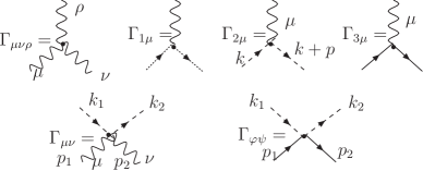
Figure 1: Vertices for the CS field coupled to matter. Charges flow in opposite direction to the indicated.

respectively, and of the vertices (see Fig. 1):

$$\Gamma_{\mu\nu\rho} = 2ie\,\epsilon_{\mu\nu\rho}\,\sin(k\wedge p),$$ (10)

$$\Gamma_{1\mu} = -2ek_{\mu}\sin(k\wedge p).$$ (11)

The graphical correspondence for the other vertices depends on the representation. To distinguish the same vertex in the fundamental and adjoint representations we include an additional index $F$ and $A$, respectively. Thus to the trilinear scalar-gauge field vertex, indicated by $\Gamma_{2\mu}$ in Fig. 1 corresponds

$$\Gamma^{F}_{2\mu}=-ie(2k+p)_{\mu}\,{\rm e}^{-ik\wedge p},$$ (12)

for the fundamental representation and

$$\Gamma^{A}_{2\mu}=2e(2k+p)_{\mu}\,\sin(k\wedge p),$$ (13)

for the adjoint representation. Using this convention the other vertices are

$$\Gamma^{F}_{\mu\nu} = -2ie^{2}g_{\mu\nu}{\rm e}^{-ik_{1}\wedge k_{2}}\cos(p_{1}\wedge p_{2}),$$ (14)

$$\Gamma^{A}_{\mu\nu} = 4ie^{2}g_{\mu\nu}\sin(k_{1}\wedge p_{1})\sin(k_{2}\wedge p_{2})+(p_{1}\leftrightarrow p_{2}),$$ (15)

$$\Gamma^{F}_{3\mu} = -e\gamma_{\mu}{\rm e}^{ik\wedge p},$$ (16)

$$\Gamma^{A}_{3\mu} = 2ie\gamma_{\mu}\sin(k\wedge p).$$ (17)

From these rules, the ultraviolet degree of superficial divergence of a generic diagram $\gamma$ turns out to be

$$d(\gamma)=3-N_{A}-N_{\psi}-\frac{1}{2}N_{\varphi}-\frac{1}{2}N_{c},$$ (18)

where $N_{A},N_{\varphi}$, $N_{\psi}$ and $N_{c}$ indicate the numbers of gauge, scalar, fermionic and ghost external lines of $\gamma$ (up to one loop $N_{c}=0$).

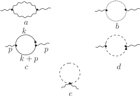
Figure 2: One-loop corrections to the gauge field two point vertex function.

A simplifying property shared by these models is the cancellation of the pure gauge contributions. Thus, when computing the corrections to the gauge field two point vertex function, one finds that the diagrams in Figs. 2$a$ and 2$b$ mutually cancel Schweda .

Concerning the possibility of the appearance of nonintegrable infrared singularities special care should be given to graphs with $d(\gamma)>0$. They can occur in the two point vertex functions of the basic fields, in the three point vertex function $<TA_{\mu}\varphi^{\dagger}\varphi>$ and in the four point vertex function $<T\varphi^{\dagger}\varphi^{\dagger}\varphi\varphi>$. In what follows we will restrict our attention to the investigation on the possibility of occurrence of nonintegrable infrared singularities.

III Fundamental representation

Let us begin our analysis by considering first the case of the fundamental representation. In this situation the one-loop contributions to the two point functions come from planar graphs and so do not induce infrared nonintegrable singularities. Thus, up to one loop the model whose action is $S_{gauge}+S_{fermion}$ is renormalizable and free from dangerous UV/IR mixing.

For the scalar model described by the action $S_{gauge}+S_{scalar}$ we need to examine the contributions to the three and four point vertex functions. We have:

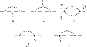
Figure 3: One-loop corrections to the gauge-scalar field three point functions.

1. Three point vertex function. The relevant diagrams are depicted in Fig. 3. Because of properties of the Levi-Cività symbol, the divergent parts of the integrals associated with the graphs in the Figs. 3$a$, 3$b$ and 3$c$ actually vanish.

Furthermore, due to our gauge choice the graphs 3$d$ and 3$e$ turn out to be only logarithmically divergent and generate a mild (integrable) infrared divergence.

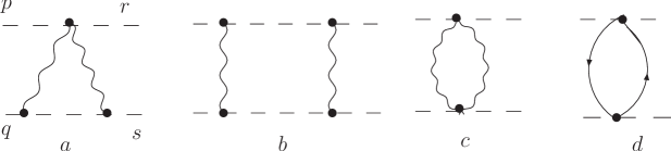
Figure 4: One-loop contributions to the four point function.

2. Four point vertex function $<T\varphi^{\dagger}\varphi\varphi^{\dagger}\varphi>$. There are three types of diagrams as drawn in Figs. 4$a-c$. In the Landau gauge, the diagrams in Figs. 4$a$ and 4$b$ are finite but graph 4$c$ presents a linear infrared divergence as can be seen from its analytical expression

$${\rm Fig4c}=-2e^{4}{\rm e}^{i(q\wedge s+p\wedge r)}\int\frac{d^{3}k}{(2\pi)^{3}}\frac{\epsilon_{\mu\rho\nu}k^{\rho}}{k^{2}}\frac{\epsilon^{\nu\alpha\mu}(k+p-r)_{\alpha}}{(k+p-r)^{2}}\cos^{2}[k\wedge(p-r)].$$ (19)

Using $\cos^{2}\phi=\frac{1}{2}[1+\cos(2\phi)]$, we obtain the following nonplanar part

$$({\rm Fig4c})_{nplanar} = -2e^{4}{\rm e}^{i(q\wedge s+p\wedge r)}\int\frac{d^{3}k}{(2\pi)^{3}}\frac{k\cdot(k+p-r)}{k^{2}(k+p-r)^{2}}\cos[2k\wedge(p-r)]$$ (20)

$$= \frac{ie^{4}}{2\pi|\tilde{p}-\tilde{r}|}+\mbox{finite term}$$

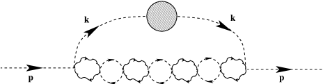
Figure 5: Nonintegrable singularity generated by iteration of the graph in Fig. 4$c$.

where in the last line $p\simeq r$. Of course, “finite term” designates the contributions that stay finite when $p\rightarrow r$. Although innocuous at this point the above infrared linear divergence ruins the perturbative expansion as it is illustrated by the graph in Fig. 5, which presents a strong nonintegrable singularity at $k=p$. To cancel such singularity we enlarge the model by coupling a fermionic field to the scalar field through the following Yukawa like self-interaction

$$S_{Yukawa}=g\int d^{3}x[\overline{\psi}\ast\psi\ast\varphi^{\dagger}\ast\varphi-\varphi^{\dagger}\ast\psi\ast\overline{\psi}\ast\varphi].$$ (21)

The relative minus sign between the terms in this expression was chosen so that it provides a mechanism for the cancellation of the infrared singularity and does not vanish in the commutative limit. To see how this happens notice that this interaction generates the vertex $\Gamma_{\varphi\psi}$ indicated in Fig. 1,

$$\Gamma_{\varphi\psi}=2ig\cos(k_{1}\wedge k_{2}+p_{1}\wedge p_{2}).$$ (22)

Among the new diagrams produced by this new interaction we have the graph in Fig. 4$d$ which gives the nonplanar contribution

$$({\rm Fig4d})_{nplanar}=-2g^{2}\!\int\frac{d^{3}k}{(2\pi)^{3}}\frac{-k\cdot(k+p-r)+m^{2}}{[(k+p-r)^{2}+M^{2}](k^{2}+M^{2})}\cos[2k\wedge(p-r)+p\wedge r-q\wedge s],$$ (23)

from which we obtain the following divergent part as $p\to r$:

$$\mbox{Divergent part of $({\rm Fig4d})_{nplanar}$}=-\frac{ig^{2}}{2\pi|\tilde{p}-\tilde{r}|}$$ (24)

so that, to cancel the divergence in ${(\rm Fig4c)}_{nplanar}$, we must set $g=e^{2}$.

We can check that all one-loop additional diagrams containing the vertex (21) do not generate nonintegrable singularities. Therefore, we may conclude that the model whose action is

$$S_{gauge}+S_{scalar}+S_{fermion}+S_{Yukawa}$$ (25)

is free from dangerous infrared divergences if $g=e^{2}$.

IV Adjoint representation

Let us now examine the models introduced in the previous section but with the matter fields in the adjoint representation. We begin the analysis by considering the model with action $S_{gauge}+S_{fermion}$. In this case the graphs contributing to the two point proper vertex functions are no longer purely planar. Actually we have:

1. Gauge field two point proper vertex function. The relevant diagram is the graph in Fig. 2$c$ which yields

$$\pi^{\mu\nu}_{f}(p) = -4e^{2}\int\frac{d^{3}k}{(2\pi)^{3}}{\textrm{Tr}}[\gamma^{\nu}\frac{i}{-i\not\!k+M}\gamma^{\mu}\frac{i}{-i(\not\!k+\not\!p)+M}]\sin^{2}{(k\wedge p)}$$ (26)

$$= \pi^{\mu\nu}_{f,\,planar}(p)+\pi^{\mu\nu}_{f,\,nplanar}(p),$$

where the subscript $f$ designates the fermionic contribution and the planar and nonplanar parts are ($a=\sqrt{M^{2}+x(1-x)p^{2}}$)

$$\pi^{\mu\nu}_{f,planar}=-\frac{ie^{2}}{\pi}(g^{\mu\nu}p^{2}-p^{\mu}p^{\nu})\int_{0}^{1}dx\frac{x(1-x)}{a}+\frac{Me^{2}}{2\pi}\epsilon^{\mu\nu\rho}p_{\rho}\int_{0}^{1}dx\frac{1}{a}$$ (27)

and

$$\!\!\!\!\!\!\!\!\!\!\!\!\!\!\!\!\!\!\!\!\!\!\!\!\!\!\!\!\!\!\pi^{\mu\nu}_{f,\,nplanar}(p)=\frac{ie^{2}}{\pi}(g^{\mu\nu}p^{2}-p^{\mu}p^{\nu})\int_{0}^{1}dx\frac{x(1-x)}{a}{\rm e}^{-a\sqrt{\tilde{p}^{2}}}$$

$$+\frac{ie^{2}}{\pi}\frac{\tilde{p}^{\mu}\tilde{p}^{\nu}}{\tilde{p}^{2}}\int_{0}^{1}dx(a+\frac{1}{\sqrt{\tilde{p}^{2}}}){\rm e}^{-a\sqrt{\tilde{p}^{2}}}-\frac{Me^{2}}{2\pi}\epsilon^{\mu\nu\rho}p_{\rho}\int_{0}^{1}dx\frac{1}{a}{\rm e}^{-a\sqrt{\tilde{p}^{2}}},$$ (28)

which diverges linearly as $p\rightarrow 0$. To cancel this divergence we add scalar fields described by the action in Eq. (2) but with mass $m=M$. We then have the contributions from the graphs in Figs. 2$d$ and 2$e$ which give

$$\pi_{b}^{\mu\nu}(p)=-\frac{ie^{2}}{4\pi} \left\{(g^{\mu\nu}p^{2}-p^{\mu}p^{\nu})\int_{0}^{1}dx\frac{(1-2x)^{2}}{a}(1-{\textrm{e}}^{-a\sqrt{\tilde{p}^{2}}})\right.$$ (29)

$$\left.+4\frac{\tilde{p}^{\mu}\tilde{p}^{\nu}}{\tilde{p}^{2}}\int_{0}^{1}dx(\frac{1}{\sqrt{\tilde{p}^{2}}}+a){\textrm{e}}^{-a\sqrt{\tilde{p}^{2}}}\right\}.$$

As we see, this last expression presents the same infrared divergence as in the fermion case. Thus, as the masses are equal the two divergences cancel.

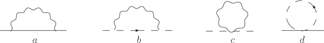
Figure 6: One-loop corrections to the matter fields two point functions

Let us now consider the one-loop corrections to the two point vertex functions of the matter fields. Up to this point, the relevant diagrams are depicted in Fig. 6($a-c$). In the Landau gauge the integrands for the diagrams 6$b$ and 6$c$ vanish, so that the two point vertex function of the scalar field does not introduce nonintegrable infrared singularities. Concerning the two point vertex function of the fermion field, after a straightforward simplification, the graph in 6$a$ furnishes

$$\Sigma_{\psi}=4ie^{2}\int\frac{d^{3}k}{(2\pi)^{3}}\frac{\not k\left[i(k-p)_{\beta}\gamma^{\beta}+m\right]}{k^{2}[(k-p)^{2}+m^{2})]}[1-\cos(2k\wedge p)],$$ (30)

whose nonplanar part yields

$$\Sigma_{\psi\,\,nplanar}=4e^{2}\int\frac{d^{3}k}{(2\pi)^{3}}\frac{\cos(2k\wedge p)}{(k^{2}+m^{2})}+\mbox{finite term}=-\frac{ie^{2}}{\pi\sqrt{\tilde{p}^{2}}}{\rm e}^{-m\sqrt{\tilde{p}^{2}}}+\mbox{finite term}.$$ (31)

To keep things in perspective, we should recall that, besides this divergence we need also to cancel the one associated with the four point function $<T\varphi^{\dagger}\varphi\varphi^{\dagger}\varphi>$. Before adding fermions this function receives contribution from the diagram in the Fig. 4$c$. In the adjoint representation this graph gives

$${\rm Fig4c}=-8e^{4}\int\frac{d^{3}k}{(2\pi)^{3}}\frac{\epsilon_{\mu\rho\nu}k^{\rho}}{k^{2}}\frac{\epsilon^{\nu\alpha\mu}(k+p-r)_{\alpha}}{(k+p-r)^{2}}{\cal C}=-16e^{4}\int\frac{d^{3}k}{(2\pi)^{3}}\frac{(k+p-r)\cdot k}{(k+p-r)^{2}k^{2}}{\cal C}$$ (32)

where ${\cal C}$ is the trigonometric factor

$${\cal C} = [\sin(k\wedge q+s\wedge q)\sin(k\wedge s)+\sin(k\wedge q)\sin(k\wedge s+s\wedge q)]$$ (33)

$$\times[\sin(k\wedge r+p\wedge r)\sin(k\wedge p)+\sin(k\wedge r)\sin(k\wedge p+p\wedge r)].$$

As done in our study of the fundamental representation, we investigate the possibility to cancel these divergences by adding a Yukawa like interaction. The structure of the trigonometric factor in Eq. (33) suggests that one should include the interaction

$$S_{Yukawa,\,adjoint}=g_{1}\int d^{3}x\{[\varphi^{\dagger},\,\psi\,]_{*}\ast[\varphi,\,\overline{\psi}]_{*}-[\varphi^{\dagger},\,\overline{\psi}\,]_{*}\ast[\varphi,\,\psi]_{*}\}.$$ (34)

In fact, this interaction introduces a new vertex which will be still represented by the last vertex in Fig. 1 but which corresponds to

$$\Gamma_{1\varphi\psi}=4ig_{1}[\sin(k_{1}\wedge p_{1})\sin(k_{2}\wedge p_{2})+\sin(k_{1}\wedge p_{2})\sin(k_{2}\wedge p_{1})].$$ (35)

Because of this new vertex, there is one additional diagram, Fig. 6$d$, which provides the following contribution to the two point vertex function of the fermion field

$${\rm Fig6d}=8g_{1}\int\frac{d^{3}k}{(2\pi)^{3}}\frac{\sin^{2}(k\wedge p)}{k^{2}+m^{2}}.$$ (36)

As the nonplanar part of this graph is equal to

$$({\rm Fig6d})_{nplanar}=-4g_{1}\int\frac{d^{3}k}{(2\pi)^{3}}\frac{\cos(2k\wedge p)}{(k^{2}+m^{2})}=\frac{ig_{1}}{\pi\sqrt{\tilde{p}^{2}}}{\rm e}^{-m\sqrt{\tilde{p}^{2}}},$$ (37)

we see that the infrared singularity will cancel if $g_{1}=e^{2}$.

Concerning the four point proper function of the scalar field, notice that there is also a new diagram which topologically is the same as the graph in Fig. 4$d$ but whose analytical expression is

$${\rm Fig4d} = 16g_{1}^{2}\int\frac{d^{3}k}{(2\pi)^{3}}{\rm Tr}[\Delta_{\psi}(k)\Delta_{\psi}(k+p-r)]{\cal C}$$ (38)

$$= -32g_{1}^{2}\int\frac{d^{3}k}{(2\pi)^{3}}\frac{-k\cdot(k+p-r)+m^{2}}{[(k+p-r)^{2}+m^{2}][k^{2}+m^{2}]}{\cal C}.$$

As $g_{1}=e^{2}$ the two contributions, Eqs. (32) and (38), do not cancel and a linear IR divergence persists. To remove such divergence a further extension of the model is needed. Taking into account these observations, in the next section we will consider a superfield CS model.

V the superfield CS model

We begin our analysis by considering the 2+1 dimensional superfield CS model which is defined by the action SGRS

$$S=m\int d^{5}z(A^{\alpha}*W_{\alpha}+\frac{i}{6}\{A^{\alpha},A^{\beta}\}_{\ast}\ast D_{\beta}A_{\alpha}+\frac{1}{12}\{A^{\alpha},A^{\beta}\}_{\ast}*\{A_{\alpha},A_{\beta}\}_{\ast})\,,$$ (39)

where

$$W_{\beta}=\frac{1}{2}D^{\alpha}D_{\beta}A_{\alpha}-\frac{i}{2}[A^{\alpha},D_{\alpha}A_{\beta}]_{\ast}-\frac{1}{6}[A^{\alpha},\{A_{\alpha},A_{\beta}\}_{\ast}]_{\ast}$$ (40)

is a superfield strength constructed from the spinor superpotential $A_{\alpha}$. This action is invariant under the infinitesimal gauge transformations

$$\delta A_{\alpha}=D_{\alpha}K-i[A_{\alpha},K]_{\ast}\,,$$ (41)

where $K$ is a scalar superfield parameter. As a first step for quantization, we eliminate this gauge freedom by choosing the gauge fixing and associate Faddeev-Popov terms as specified by the action

$$S_{GF+FP}=-\frac{m}{2\xi}\int d^{5}z(D^{\alpha}A_{\alpha})(D^{\beta}A_{\beta})+\frac{1}{2g^{2}}\int d^{5}z(c^{\prime}D^{\alpha}D_{\alpha}c+ic^{\prime}*D^{\alpha}[A_{\alpha},c]_{\ast})\,,$$ (42)

so that the quadratic part of the action reads

$$S_{2}=-\frac{1}{2}m\int d^{5}zA_{\beta}\Big{[}D^{\alpha}D^{\beta}+\frac{1}{\xi}D^{\beta}D^{\alpha}\Big{]}A_{\alpha}+\frac{1}{2g^{2}}\int d^{5}zc^{\prime}D^{\alpha}D_{\alpha}c\,.$$ (43)

From this action we get the free gauge and ghost propagators as being

$$<A^{\alpha}(z_{1})A^{\beta}(z_{2})>=\frac{i}{4m\Box}\left[D^{\beta}D^{\alpha}+\xi D^{\alpha}D^{\beta}\right]\delta^{5}(z_{1}-z_{2})\,,$$ (44)

and

$$<c^{\prime}(z_{1})c(z_{2})>=-ig^{2}\frac{D^{2}}{\Box}\delta^{5}(z_{1}-z_{2})\,.$$ (45)

The interaction part of the action determines three types of vertices:

$$\Gamma_{3} = a_{3}mA^{\beta}(k_{1})A^{\alpha}(k_{2})D_{\alpha}A_{\beta}(k_{3})\sin(k_{2}\wedge k_{3}),$$

$$\Gamma_{4} = a_{4}mA^{\beta}(k_{1})A^{\alpha}(k_{2})A_{\alpha}(k_{3})A_{\beta}(k_{4})\sin(k_{1}\wedge k_{2})\sin(k_{3}\wedge k_{4}),$$

$$\Gamma_{c} = -\frac{1}{g^{2}}c^{\prime}(k_{1})D^{\alpha}(A_{\alpha}(k_{2})c(k_{3}))\sin(k_{2}\wedge k_{3}),$$ (46)

where $a_{3}=\frac{2}{3}$ and $a_{4}=\frac{1}{3}$. Instead of writing their explicit values, we will retain the notations $a_{3}$ and $a_{4}$ to keep track of the contributions of each vertex.

To study the divergence structure of the model we shall start by determining the superficial degree of divergence $d(\gamma)$ associated to a generic supergraph $\gamma$. Explicitly, $d(\gamma)$ receives contributions from the propagators and, implicitly, from the supercovariant derivatives. This last dependence can be unveiled by the use of the conversion rule

$$D_{\alpha}(-k,\theta)D_{\beta}(-k,\theta)=k_{\alpha\beta}-C_{\alpha\beta}D^{2}(-k,\theta)$$ (47)

and the identity $(D^{2})^{2}=-k^{2}$. Let $V_{1}$ be the number of pure gauge vertices containing one super-derivative and $V_{c}$ the number of ghost vertices; let $P_{A}$ and $P_{c}$ be the numbers of gauge and ghost superpropagators and let $N_{D}$ be the number of supercovariant derivatives that act on the external lines after the usual D-algebra transformations. The superficial degree of divergence is then

$$d(\gamma)=2L+\frac{1}{2}(V_{1}+V_{c})-P_{A}-P_{c}-\frac{1}{2}N_{D}\,,$$ (48)

where $L$ is the number of loops. As we are going to consider Green functions of the gauge superfield only, then $V_{c}=P_{c}$. Using this and the topological identity relating the number of lines, the number of vertices and the number of loops, the above formula can be rewritten as

$$d(\gamma)=2-\frac{1}{2}E_{A}-\frac{1}{2}N_{D},$$ (49)

where $E_{A}$ denotes the number of external $A$ lines.

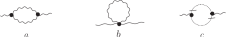
Figure 7: Superficially linearly divergent diagrams contributing to the two-point function of the gauge superfield.

At one loop, due to symmetric integration, the superficially logarithmically divergent contributions are actually finite. We have therefore to examine only graphs that are potentially linearly divergent. They contribute to the two point gauge superfield vertex function and are depicted in Fig. 7. First notice that the ghost contribution in Fig. 7$c$ is the same as in noncommutative super-QED₃ so that we just quote the result from ours

$$\Gamma_{2c}=-\frac{1}{2}\int\frac{d^{3}p}{(2\pi)^{3}}d^{2}\theta_{1}\int\frac{d^{3}k}{(2\pi)^{3}}\frac{\sin^{2}(k\wedge p)}{k^{2}}A^{\beta}(-p,\theta_{1})A_{\beta}(p,\theta_{1})\,+\,\cdots\,,$$ (50)

where the ellipsis stands for finite terms. The second contribution, which comes from the tadpole graph in Fig. 7$b$, is also easily evaluated giving

$$\Gamma_{2b}=\frac{3}{2}a_{4}(1-\xi)\int\frac{d^{3}p}{(2\pi)^{3}}d^{2}\theta_{1}\int\frac{d^{3}k}{(2\pi)^{3}}\frac{\sin^{2}(k\wedge p)}{k^{2}}A^{\beta}(-p,\theta_{1})A_{\beta}(p,\theta_{1}).$$ (51)

The evaluation of the graph in Fig. 7$a$ is more complicated as it involves two types of contractions distinguished by the fact that the two derivatives at the vertices act on the same line (denoted by $(a)$, $(b)$ and $(c)$) or on different lines (indicated by $(a^{\prime})$, $(b^{\prime})$ and $(c^{\prime})$):

$$\Gamma_{2a}=(a)+(b)+(c)+(a^{\prime})+(b^{\prime})+(c^{\prime})$$ (52)

where

$$(a) = {m^{2}}a^{2}_{3}\int\frac{d^{3}p}{(2\pi)^{3}}d^{2}\theta_{1}d^{2}\theta_{2}\int\frac{d^{3}k}{(2\pi)^{3}}\sin^{2}(k\wedge p)<D_{\alpha}A_{\beta}(k,\theta_{1})D_{\alpha^{\prime}}A_{\beta^{\prime}}(-k,\theta_{2})>$$

$$\times <A^{\beta}(p-k,\theta_{1})A^{\alpha^{\prime}}(-(p-k),\theta_{2})>A^{\alpha}(-p,\theta_{1})A^{\beta^{\prime}}(p,\theta_{2}),$$

$$(b) = \frac{m^{2}}{2}a^{2}_{3}\int\frac{d^{3}p}{(2\pi)^{3}}d^{2}\theta_{1}d^{2}\theta_{2}\int\frac{d^{3}k}{(2\pi)^{3}}\sin^{2}(k\wedge p)<D_{\alpha}A_{\beta}(k,\theta_{1})D_{\alpha^{\prime}}A_{\beta^{\prime}}(-k,\theta_{2})>$$

$$\times <A^{\beta}(p-k,\theta_{1})A^{\beta^{\prime}}(-(p-k),\theta_{2})>A^{\alpha}(-p,\theta_{1})A^{\alpha^{\prime}}(p,\theta_{2}),$$

$$(c) = \frac{m^{2}}{2}a^{2}_{3}\int\frac{d^{3}p}{(2\pi)^{3}}d^{2}\theta_{1}d^{2}\theta_{2}\int\frac{d^{3}k}{(2\pi)^{3}}\sin^{2}(k\wedge p)<D_{\alpha}A_{\beta}(k,\theta_{1})D_{\alpha^{\prime}}A_{\beta^{\prime}}(-k,\theta_{2})>$$ (53)

$$\times <A^{\alpha}(p-k,\theta_{1})A^{\alpha^{\prime}}(-(p-k),\theta_{2})>A^{\beta}(-p,\theta_{1})A^{\beta^{\prime}}(p,\theta_{2}),$$

$$(a^{\prime}) = m^{2}a^{2}_{3}\int\frac{d^{3}p}{(2\pi)^{3}}d^{2}\theta_{1}d^{2}\theta_{2}\int\frac{d^{3}k}{(2\pi)^{3}}\sin^{2}(k\wedge p)<D_{\alpha}A_{\beta}(k,\theta_{1})A^{\alpha^{\prime}}(-k,\theta_{2})>$$

$$\times <A^{\beta}(p-k,\theta_{1})D_{\alpha^{\prime}}A_{\beta^{\prime}}(-(p-k),\theta_{2})>A^{\alpha}(-p,\theta_{1})A^{\beta^{\prime}}(p,\theta_{2}),$$

$$(b^{\prime}) = \frac{m^{2}}{2}a^{2}_{3}\int\frac{d^{3}p}{(2\pi)^{3}}d^{2}\theta_{1}d^{2}\theta_{2}\int\frac{d^{3}k}{(2\pi)^{3}}\sin^{2}(k\wedge p)<D_{\alpha}A_{\beta}(k,\theta_{1})A^{\beta^{\prime}}(-k,\theta_{2})>$$

$$\times <A^{\beta}(p-k,\theta_{1})D_{\alpha^{\prime}}A_{\beta^{\prime}}(-(p-k),\theta_{2})>A^{\alpha}(-p,\theta_{1})A^{\alpha^{\prime}}(p,\theta_{2}),$$

$$(c^{\prime}) = \frac{m^{2}}{2}a^{2}_{3}\int\frac{d^{3}p}{(2\pi)^{3}}d^{2}\theta_{1}d^{2}\theta_{2}\int\frac{d^{3}k}{(2\pi)^{3}}\sin^{2}(k\wedge p)<D_{\alpha}A_{\beta}(k,\theta_{1})A^{\alpha^{\prime}}(-k,\theta_{2})>$$ (54)

$$\times <A^{\alpha}(p-k,\theta_{1})D_{\alpha^{\prime}}A_{\beta^{\prime}}(-(p-k),\theta_{2})>A^{\beta}(-p,\theta_{1})A^{\beta^{\prime}}(p,\theta_{2}).$$

After straightforward D-algebra transformations we obtain

$$(a) = 8a^{2}_{3}\xi\int d^{2}\theta\int\frac{d^{3}pd^{3}k}{(2\pi)^{6}}Jk^{2}A^{\beta}(-p,\theta)A_{\beta}(p,\theta),$$

$$(b) = 8a^{2}_{3}\xi\int d^{2}\theta\int\frac{d^{3}pd^{3}k}{(2\pi)^{6}}Jk^{2}A^{\beta}(-p,\theta)A_{\beta}(p,\theta),$$

$$(c) = 4a^{2}_{3}(\xi-\xi^{2})\int d^{2}\theta\int\frac{d^{3}pd^{3}k}{(2\pi)^{6}}Jk^{2}A^{\beta}(-p,\theta)A_{\beta}(p,\theta),$$

$$(a^{\prime}) = 8a^{2}_{3}\xi\int d^{2}\theta\int\frac{d^{3}pd^{3}k}{(2\pi)^{6}}Jk^{2}A^{\beta}(-p,\theta)A_{\beta}(p,\theta),$$

$$(b^{\prime}) = 8a^{2}_{3}\xi\int d^{2}\theta\int\frac{d^{3}pd^{3}k}{(2\pi)^{6}}Jk^{2}A^{\beta}(-p,\theta)A_{\beta}(p,\theta),$$

$$(c^{\prime}) = 4a^{2}_{3}\xi^{2}\int d^{2}\theta\int\frac{d^{3}pd^{3}k}{(2\pi)^{6}}Jk^{2}A^{\beta}(-p,\theta)A_{\beta}(p,\theta),$$ (55)

where

$$J=\frac{1}{32}\frac{\sin^{2}(k\wedge p)}{k^{2}(p-k)^{2}}.$$ (56)

The final contribution of this graph is therefore

$$\Gamma_{2a}=\frac{9}{8}a^{2}_{3}\xi\int\frac{d^{3}p}{(2\pi)^{3}}d^{2}\theta\int\frac{d^{3}k}{(2\pi)^{3}}\frac{\sin^{2}(k\wedge p)}{k^{2}}A^{\beta}(-p,\theta)A_{\beta}(p,\theta).$$ (57)

Thus, collecting the results in (50), (51) and (57) we get that the would be divergent part of $\Gamma_{2}$,

$$\Gamma_{2}^{Div}=(\frac{9}{8}a^{2}_{3}\xi+\frac{3}{2}a_{4}(1-\xi)-\frac{1}{2})\int\frac{d^{3}p}{(2\pi)^{3}}d^{2}\theta\int\frac{d^{3}k}{(2\pi)^{3}}\frac{\sin^{2}(k\wedge p)}{k^{2}}A^{\beta}(-p,\theta)A_{\beta}(p,\theta),$$ (58)

vanishes irrespectively of the gauge parameter $\xi$. This means that the one-loop two point vertex function of the gauge superfield is free from both UV and UV/IR infrared singularities in any covariant gauge. As a matter of fact, using arguments similar to those presented in ours one can demonstrate that all superficially logarithmically divergent graphs are finite. We therefore conclude that in any gauge the model is one-loop finite.

Let us now consider the effect of the inclusion of matter fields. We first examine the case in which a scalar superfield in the adjoint representation couples to the CS superfield through the action

$$S^{A} = \int d^{5}z\Big{\{}\bar{\phi}(D^{2}-M)\phi-\frac{i}{2}(g[\bar{\phi},A^{\alpha}]_{*}*D_{\alpha}\phi-gD^{\alpha}\bar{\phi}*[A_{\alpha},\phi]_{*})$$ (59)

$$-\frac{g^{2}}{2}[\bar{\phi},A^{\alpha}]_{*}*[A_{\alpha},\phi]_{*}\Big{\}}.$$

With this modification the superficial degree of divergence in Eq. (49) must be replaced by

$$d(\gamma)=2-\frac{1}{2}(E_{A}+E_{\phi})-\frac{N_{D}}{2},$$ (60)

where $E_{A}$ and $E_{\phi}$ are the numbers of the external $A$ and $\phi$ lines, respectively. The more dangerous situations correspond to linearly divergent contributions which are possible only if $E_{\phi}=2$ or $E_{A}=2$. The addition of the action (59) generates new contributions to the two point proper vertex function of the gauge superfield. The corresponding supergraphs are listed in Fig. 8 and the details of their computation are the same as in the three-dimensional noncommutative $CP^{N-1}$ model cpn . They give the following contributions to the effective action

$$iS^{A}_{8a}(p) = -2g^{2}\int d^{2}\theta\int\frac{d^{3}k}{(2\pi)^{3}}I(k,p)$$ (61)

$$\times \Big{[}(k^{2}+M^{2})C_{\alpha\beta}A^{\alpha}(-p,\theta)A^{\beta}(p,\theta)+(k_{\alpha\beta}+MC_{\alpha\beta})(D^{2}A^{\alpha}(-p,\theta))A^{\beta}(p,\theta)$$

$$+ \frac{1}{2}D^{\gamma}D^{\alpha}A_{\alpha}(-p,\theta)(k_{\gamma\beta}+MC_{\gamma\beta})A^{\beta}(p,\theta)\Big{]}$$

and

$$iS^{A}_{8b}(p) = 2g^{2}\int\frac{d^{3}k}{(2\pi)^{3}}\frac{\sin^{2}(k\wedge p)}{(k+p)^{2}+M^{2}}C_{\alpha\beta}A^{\alpha}(-p,\theta)A^{\beta}(p,\theta),$$ (62)

where

$$I(k,p)=\frac{\sin^{2}(k\wedge p)}{(k^{2}+M^{2})[(k+p)^{2}+M^{2}]}.$$ (63)

Although individually divergent the sum of $iS^{A}_{8a}(p)$ and $iS^{A}_{8b}(p)$ is finite being equal to

$$iS^{A}_{8}(p) = -2g^{2}\int d^{2}\theta\int\frac{d^{3}k}{(2\pi)^{3}}I(k,p)$$ (64)

$$\times (k_{\gamma\beta}+MC_{\gamma\beta})\Big{[}(D^{2}A^{\gamma}(-p,\theta))A^{\beta}(p,\theta)+\frac{1}{2}D^{\gamma}D^{\alpha}A_{\alpha}(-p,\theta)A^{\beta}(p,\theta)\Big{]},$$

or equivalently,

$$S^{A}_{8}(p) = \frac{g^{2}}{16\pi}\int d^{2}\theta f(p)A^{\beta}(p,\theta)[D^{2}+2M]W_{0\beta}(-p,\theta)$$ (65)

$$= \frac{g^{2}}{16\pi}\int d^{2}\theta f(p)[W_{0}^{\alpha}W_{0\alpha}+2MW^{\alpha}_{0}A_{\alpha}],$$

where

$$f(p)=-16\pi i\int\frac{d^{3}k}{(2\pi)^{3}}I(k,p)$$ (66)

and $W^{\alpha}_{0}=\frac{1}{2}D^{\beta}D^{\alpha}A_{\beta}$ is a linearized superfield strength. As we see, these graphs originate nonlocal Maxwell and CS terms in the effective action.

Let us now consider the two point function of the scalar superfield. The one-loop contributing graphs are depicted in Fig. 9; they are superficially linearly divergent. Notice that, as before by reasons of symmetry, the would be logarithmic divergences vanish and therefore all terms which do not contain linear divergences are finite.

The UV leading part of the graph in Fig. 9$a$, which involves two vertices with three fields is

$$iS^{(1)A}_{\phi\bar{\phi}} = -\frac{1}{2}g^{2}\int\frac{d^{3}k}{(2\pi)^{3}}\int d^{2}\theta_{1}d^{2}\theta_{2}\frac{\sin^{2}(k\wedge p)}{4mk^{2}[(p+k)^{2}+M^{2}]}(D^{\beta}D^{\alpha}+\xi D^{\alpha}D^{\beta})\delta_{12}$$ (67)

$$\times D_{\alpha 1}(D^{2}+M)D_{\beta 2}\delta_{12}[\phi(-p,\theta_{1})\bar{\phi}(p,\theta_{2})+\bar{\phi}(-p,\theta_{1})\phi(p,\theta_{2})]$$

and, after D-algebra transformations turns out to be

$$iS^{(1)A}_{\phi\bar{\phi}}=\xi g^{2}\int d^{2}\theta\frac{\phi(-p,\theta)\bar{\phi}(p,\theta)}{m}\int\frac{d^{3}k}{(2\pi)^{3}}\frac{\sin^{2}(k\wedge p)}{k^{2}}+\mbox{finite term}.$$ (68)

Notice that this gauge dependent contribution only vanishes in the Landau, $\xi=0$ gauge, as could be anticipated from a rapid inspection of Eq. (67). Now, after trivial D-algebra transformations the contribution from the graph in Fig. 9$b$ becomes

$$iS^{(2)A}_{\phi\bar{\phi}}=-(1-\xi)g^{2}\int d^{2}\theta\frac{\phi(-p,\theta)\bar{\phi}(p,\theta)}{m}\int\frac{d^{3}k}{(2\pi)^{3}}\frac{\sin^{2}(k\wedge p)}{k^{2}}+\mbox{finite term}.$$ (69)

Differently from Eq. (68) the above result only vanishes in the Feynman, $\xi=1$, gauge where the propagator of the $A^{\alpha}$ superfield does not contain spinor derivatives. The sum of Eqs. (68) and (69) only vanishes in the $\xi=1/2$ gauge and thus only in this gauge the model with the matter superfields in the adjoint representation is free from dangerous UV/IR infrared divergences.

A more favorable situation occurs if the matter superfield belongs to the fundamental representation of the gauge group. In this case the matter action is

$$S^{F} = \int d^{5}z\Big{[}\bar{\phi}(D^{2}-M)\phi-\frac{ig}{2}(\bar{\phi}*A^{\alpha}*D_{\alpha}\phi-D^{\alpha}\bar{\phi}*A_{\alpha}*\phi)$$ (70)

$$-\frac{g^{2}}{2}\bar{\phi}*A^{\alpha}*A_{\alpha}*\phi\Big{]},$$

which implies in the following form of the vertices after the Fourier transform:

$$\Gamma^{F}_{3} = -\frac{ig}{2}A^{\alpha}(k_{1})(D_{\alpha}\phi(k_{2})\bar{\phi}(k_{3})-\phi(k_{2})D_{\alpha}\bar{\phi}(k_{3}))e^{ik_{2}\wedge k_{3}},$$

$$\Gamma^{F}_{4} = -\frac{g^{2}}{2}\bar{\phi}(k_{1})A^{\alpha}(k_{2})A_{\alpha}(k_{3})\phi(k_{4})e^{ik_{1}\wedge k_{2}+ik_{3}\wedge k_{4}}.$$ (71)

We can easily calculate the contributions of graphs containing these vertices to the two point function of the gauge superfield. In fact, the D-algebra transformations are exactly the same as in the adjoint representation, the only differences in the analytical expressions being due to the replacement of trigonometric factors by phases in the way specified in the Eqs. (71). However, these phase factors do not interfere with the calculations since both graphs turn out to be planar. Their corresponding analytical expressions are

$$iS^{F}_{8a}(p) = -\frac{g^{2}}{2}\int d^{2}\theta\int\frac{d^{3}k}{(2\pi)^{3}}\frac{1}{(k^{2}+M^{2})[(k+p)^{2}+M^{2}]}$$ (72)

$$\times \Big{[}(k^{2}+M^{2})C_{\alpha\beta}A^{\alpha}(-p,\theta)A^{\beta}(p,\theta)+(k_{\alpha\beta}+MC_{\alpha\beta})(D^{2}A^{\alpha}(-p,\theta))A^{\beta}(p,\theta)$$

$$+ \frac{1}{2}D^{\gamma}D^{\alpha}A_{\alpha}(-p,\theta)(k_{\gamma\beta}+MC_{\gamma\beta})A^{\beta}(p,\theta)\Big{]}$$

and

$$iS^{F}_{8b}(p) = \frac{g^{2}}{2}\int\frac{d^{3}k}{(2\pi)^{3}}\frac{1}{(k+p)^{2}+M^{2}}C_{\alpha\beta}A^{\alpha}(-p,\theta)A^{\beta}(p,\theta).$$ (73)

Their sum is also finite and equal to

$$iS^{F}_{8}(p) = -\frac{g^{2}}{2}\int d^{2}\theta\int\frac{d^{3}k}{(2\pi)^{3}}\frac{1}{(k^{2}+M^{2})[(k+p)^{2}+M^{2}]}$$ (74)

$$\times (k_{\gamma\beta}+MC_{\gamma\beta})\Big{[}(D^{2}A^{\gamma}(-p,\theta))A^{\beta}(p,\theta)+\frac{1}{2}D^{\gamma}D^{\alpha}A_{\alpha}(-p,\theta)A^{\beta}(p,\theta)\Big{]},$$

the only difference with respect to Eq. (64) being the absence of the trigonometric factor.

We still have to examine the contributions to the two point vertex function of the scalar superfield. The relevant graphs are again those drawn in Fig. 9 and in this case are totally planar. We get

$$iS^{(1)F}_{\phi\bar{\phi}} = -\frac{1}{8}g^{2}\int\frac{d^{3}k}{(2\pi)^{3}}\int d^{2}\theta_{1}d^{2}\theta_{2}\frac{1}{4mk^{2}[(p+k)^{2}+M^{2}]}(D^{\beta}D^{\alpha}+\xi D^{\alpha}D^{\beta})\delta_{12}$$ (75)

$$\times D_{\alpha 1}(D^{2}+M)D_{\beta 2}\delta_{12}[\phi(-p,\theta_{1})\bar{\phi}(p,\theta_{2})+\bar{\phi}(-p,\theta_{1})\phi(p,\theta_{2})],$$

which after D-algebra transformations becomes

$$iS^{(1)F}_{\phi\bar{\phi}}=\frac{1}{4}g^{2}\xi\int d^{2}\theta\frac{\phi(-p,\theta)\bar{\phi}(p,\theta)}{m}\int\frac{d^{3}k}{(2\pi)^{3}}\frac{1}{k^{2}}+\mbox{finite term}.$$ (76)

The D-algebra transformations for the second graph are simpler and yield

$$iS^{(2)F}_{\phi\bar{\phi}}=-\frac{1}{4}(1-\xi)g^{2}\int d^{2}\theta\frac{\phi(-p,\theta)\bar{\phi}(p,\theta)}{m}\int\frac{d^{3}k}{(2\pi)^{3}}\frac{1}{k^{2}}.$$ (77)

In the context of dimensional regularization, which we are implicitly assuming, these divergent parts vanish. Thus in any gauge the one-loop contributions to the two point vertex function of the scalar superfield are finite. This result singles out the fundamental representation as the preferable one for the construction of the model.

It should be noticed that although absent in the one-loop corrections a quartic self-interaction of the scalar superfield may be induced at higher orders. In that situation for renormalizability one should a fortiori introduce the coupling

$$-\frac{\lambda}{2}\int d^{5}z\bar{\phi}*\phi*\bar{\phi}*\phi,$$ (78)

which in its turn generates new one-loop graphs. In particular, for the two point function of the scalar superfield we have the graph depicted in Fig. 10 which corresponds to

$$-2\lambda\int d^{2}\theta\int\frac{d^{3}p}{(2\pi)^{3}}\int\frac{d^{3}k}{(2\pi)^{3}}\frac{1}{k^{2}+M^{2}}(D^{2}+M)\delta_{11}\phi(-p,\theta)\bar{\phi}(p,\theta),$$ (79)

which after a trivial D-algebra transformation is equal to

$$-2\lambda\int d^{2}\theta\int\frac{d^{3}p}{(2\pi)^{3}}\int\frac{d^{3}k}{(2\pi)^{3}}\frac{1}{k^{2}+M^{2}}\phi(-p,\theta)\bar{\phi}(p,\theta),$$ (80)

providing a finite mass renormalization for the scalar superfield.

VI Conclusions

In this work we have studied various models of matter fields coupled to the CS field both in the fundamental and in the adjoint representation of the $U(1)$ noncommutative gauge group. Special attention was given to the occurrence of UV/IR mixing as it may generate nonintegrable infrared singularities. We began by proving that the model describing a fermionic field minimally coupled to the CS field is free from dangerous UV/IR mixing. On the other hand, the model with only a scalar field also in the fundamental representation and minimally coupled to the CS field presents a linear infrared divergence in the one-loop contribution to the four point vertex function of the matter field. We proved that it is possible to cancel such divergence by incorporating fermions interacting with the scalar field via a noncommutative Yukawa like Lagrangian. The situations are more complicated if the matter fields belong to the adjoint representation: to eliminate the UV/IR mixing in the one-loop contributions to the gauge field propagator it is necessary to consider a more general model containing both scalar and fermionic fields minimally coupled to the CS field. However, even with the addition of a Yukawa interaction it was not possible to eliminate all one-loop infrared divergences which are present in the two point vertex function of the fermionic field and also in the four point function of the scalar field. More general interactions seemed to be necessary and also motivated by results in supersymmetric gauge theories ours ; cpn we were led to study a noncommutative CS superfield coupled to matter. We first demonstrate that the pure gauge sector is finite in an arbitrary gauge. The inclusion of matter brought new features depending on the representation to which the corresponding superfield belongs. For the matter superfield in the fundamental representation of the gauge group all one-loop graphs with positive superficial degree of divergence are planar and are therefore finite in the context of dimensional regularization. However, for the matter in the adjoint representation we found that the absence of dangerous UV/IR singularities in the two point vertex function of the matter field only happens in a particular gauge, namely $\xi=1/2$.

VII Acknowledgments

This work was partially supported by Fundação de Amparo à Pesquisa do Estado de São Paulo (FAPESP) and Conselho Nacional de Desenvolvimento Científico e Tecnológico (CNPq). A. Yu. P. has been supported by FAPESP, project No. 00/12671-7.

Figure 8: Coupling to matter: contributions to the two-point function of gauge superfield.

Figure 9: Coupling to matter: contributions to the two-point function of matter field.

Figure 10: The contribution to the two-point function of matter field generated by the matter self-interaction.