Evolution of gravitational waves in the high-energy regime of brane-world cosmology

Abstract

We discuss the cosmological evolution of gravitational waves (GWs) after inflation in a brane-world cosmology embedded in five-dimensional anti-de Sitter (AdS₅) bulk spacetime. In a brane-world scenario, the evolution of GWs is affected by the non-standard cosmological expansion and the excitation of the Kaluza-Klein modes (KK-modes), which are significant in the high-energy regime of the universe. We numerically solve the wave equation of GWs in the Poincaré coordinates of the AdS₅ spacetime. Using a plausible initial condition from inflation, we find that, while the behavior of GWs in the bulk is sensitive to the transition time from inflation to the radiation dominated epoch, the amplitude of GWs on the brane is insensitive to this time if the transition occurs early enough before horizon re-entry. As a result, the amplitude of GWs is suppressed by the excitation of KK-modes which escape from the brane into the bulk, and the effect may compensate the enhancement of the GWs by the non-standard cosmological expansion. Based on this, the influence of the high-energy effects on the stochastic background of GWs is discussed.

, ,

1 Introduction

The stochastic background of gravitational waves (SBGW) generated during the accelerating phase of the early universe is one of the most fundamental predictions of the inflationary scenario and this can provide a direct way to probe the very early universe. In particular, information about extra-dimensions is expected to be imprinted on the SBGW. Motivated by recent developments in particle physics, the possibility that our universe is described by brane with three spatial dimensions embedded in a higher-dimensional space has been extensively discussed. According to this scenario, gravity propagates in the extra spatial dimensions, while the standard model particles are confined to the three dimensional brane. At low-energy scales, four-dimensional general relativity is successfully recovered and the extra-dimensional effects should be fairly small. On the other hand, at high-energy scales, the localization of gravity is not always guaranteed and a significant deviation from the standard four-dimensional theory is expected. If this is true, the SBGW can provide a direct probe of the extra-dimensional effects.

In this letter, we focus on the brane-world model proposed by Randall and Sundrum [1]. In this model, a three dimensional brane is embedded in the five dimensional anti-de Sitter (AdS₅) bulk spacetime (see Ref.[2] for a comprehensive review of this brane-world scenario). The important model parameter is the AdS₅ curvature radius $\ell$ that determines the scale on which Newton’s force law is modified. Table-top experiments on Newton’s force law impose the constraint on $\ell$ that $\ell<0.1$mm [3]. In the context of cosmology, the evolution of the universe is significantly modified by extra-dimensional effects when the Hubble horizon becomes shorter than the AdS₅ curvature scale, $H\ell>1$. Thus there is a critical frequency corresponding to the wavelength of the gravitational waves (GWs) that cross the horizon when $H\ell=1$. This frequency is given by $f_{\rm crit}=0.2$mHz$\,(0.1$mm$/\ell)^{1/2}$ [4]. Since the GWs with short wavelengths re-enter the horizon at high energies, it is expected that the SBGW above the critical frequency is crucially affected by the extra-dimensional effects. Theoretically, there are two main effects in the high-energy regime: (i) the cosmological expansion becomes slow compared with that in four-dimensional general relativity, which enhances the amplitude of the SBGW and (ii) the excitation of Kaluza-Klein modes (KK-modes) suppresses the amplitude of the GWs on the brane. An interesting point is that these two effects affect the amplitude of the SBGW in an opposite way. Thus, quantitative calculations of the effects of the KK-modes excitation are essential in predicting the spectrum of SBGW.

There have been many attempts to understand the effect of the KK-mode excitation. One way is to work with Gaussian normal coordinates [5, 6]. Using these coordinates, we have performed a numerical study of the high-energy effects and showed that the excitation of KK-modes dominates over the effect of the non-standard cosmic expansion [7]. However, the Gaussian normal coordinates have a coordinate singularity and the analysis is limited to the relatively low-energy universe $(H\ell<1)$. Recently, Ichiki and Nakamura have performed a numerical calculation in the high-energy regime $(H\ell>1)$ using a null coordinate system [8, 9]. While they reached the same conclusion as our previous study, they took the initial condition so that the perturbation is constant along a null hypersurface. At present, however, it remains unclear whether the initial condition imposed by them is appropriate for the one determined from inflation.

In this letter, we use the Poincaré coordinate system to perform numerical calculations. The main advantage of this coordinate system is that it covers the whole bulk spacetime. Using these coordinates, several analytic and semi-analytic methods ahve been proposed [10, 11, 12], which work well in the low-energy regime. Also, the quantum fluctuations in the inflationary epoch have been discussed in the Poincaré coordinate system [13, 14]. Thus, we can set more plausible initial conditions from the inflationary universe than those in the Gaussian normal coordinates.

We set up the basic equations and prepare the numerical calculation in Section 2. The numerical results are presented in Section 3. We first discuss the validity of the initial conditions. Then we attempt to construct the spectrum of SBGW in the high energy regime of the universe. Finally, Section 4 is devoted to summary and discussion.

2 Basic equations and Numerical method

2.1 Background metric and evolution equation

In the Randall-Sundrum single-brane model [1], a three-dimensional brane is embedded in five dimensional anti-de Sitter spacetime (AdS₅ bulk). In this Letter, we specifically consider the AdS₅ bulk without a black hole mass and assume that the matter content on the brane is simply described by a homogeneous and isotropic perfect fluid whose equation of state satisfies $p=w\rho$.

In our previous study [7], the Gaussian normal (GN) coordinate system

$$ds^{2}=-n^{2}(t,y)dt^{2}+a^{2}(t,y)d\mathbf{x}^{2}+dy^{2},$$ (1)

was used to solve the wave equation of GWs. In this coordinate system, the brane is located at a fixed position $y=0$. The lapse function $n(t,y)$ is related to the warp factor $a(t,y)$ through the relation, $n(t,y)=\dot{a}(t,y)/\dot{a}(t,y=0)$:

$$a(t,y) = a_{0}(t)\left\{\cosh\left(\frac{y}{\ell}\right)-\left(1+\frac{\rho(t)}{\lambda}\right)\sinh\left(\frac{y}{\ell}\right)\right\},$$ (2)

$$n(t,y) = e^{-y/\ell}+(2+3w)\,\frac{\rho}{\lambda}\,\sinh\left(\frac{y}{\ell}\right),$$ (3)

where $\ell$ is curvature scale of the AdS₅ bulk and $\lambda>0$ is the tension of the brane. The quantity $a_{0}(t)\equiv a(t,y=0)$ denotes the scale factor on brane.

Although the GN coordinates (1) are well-behaved near the brane and so it is convenient to impose the boundary condition on the brane, difficulties arise when investigating the behavior of GWs in the bulk due to the coordinate singularity at $y=y_{\rm h}(t)$, where $a(t,y_{\rm h})=0$ (Eq.(2)). This corresponds to the past null infinity of the AdS₅ spacetime. Furthermore, a space-like $t=$const. hypersurface approaches null near the coordinate singularity. Hence, a sophisticated treatment of boundary conditions near the singularity is required. As a result, the previous numerical investigation was restricted to the analysis at relatively low-energy scales.

In this paper, in order to extend our previous study to the analysis in the high-energy regime, we use the Poincaré coordinate system $(\tau,\mathbf{x},z)$. In the Poincaré coordinate system, the brane is moving in the static AdS₅ bulk [15]. The metric is given by

$$ds^{2}=\left(\frac{\ell}{z}\right)^{2}\{-d\tau^{2}+(\delta_{ij}+h_{ij})dx^{i}dx^{j}+dz^{2}\},$$ (4)

where $h_{ij}$ is the tensor perturbation satisfying the transverse and the traceless conditions. In this metric, the trajectory of the brane is described as $(\tau_{\rm b},\,z_{\rm b})$:

$$\tau_{\rm b}=T(t),\qquad z_{\rm b}=\frac{\ell}{a_{0}(t)},$$ (5)

where the variable $t$ is the cosmic time on brane, which has the same meaning of time $t$ as used in the GN metric (1). From the junction conditions, the Friedmann equation and the conservation law become [16]:

$$H^{2}(t)=\left(\frac{\dot{a_{0}}}{a_{0}}\right)^{2}=\frac{\kappa_{4}^{2}}{3}\rho\left(1+\frac{\rho}{2\lambda}\right),\qquad\dot{\rho}=-3(1+w)H\rho,\quad(\kappa_{4}^{2}=8\pi G),$$ (6)

where the dot denotes a derivative with respect to $t$ and $H$ is the Hubble parameter defined by $H\equiv\dot{a_{0}}/a_{0}$. The function $T(t)$ is given by

$$\dot{T}(t)=\frac{1}{a_{0}}\sqrt{1+(H\ell)^{2}}.$$ (7)

Hereafter, unless otherwise mentioned, we focus on the evolution of GWs during the radiation dominated epoch after inflation, i.e., $w=1/3$. In this case, the solutions for the scale factor $a_{0}(t)$ and the normalized energy density defined by $\epsilon(t)\equiv\rho(t)/\lambda$ are expressed as (e.g., [17]):

$$a_{0}(t)=a_{*}\left(\frac{2t^{2}+t\ell}{2t_{*}^{2}+t_{*}\ell}\right)^{1/4},\quad\epsilon(t)\equiv\frac{\rho(t)}{\lambda}=\frac{\ell^{2}}{8t^{2}+4t\ell}.$$ (8)

The variables $a_{*}$ and $t_{*}$ are numerical constants, whose meanings will be given in next section.

Next consider the tensor perturbation $h_{ij}$ in the metric (4). For convenience, we decompose the quantity $h_{ij}$ in spatial Fourier modes as $h_{ij}=h_{k}(\tau,z)e^{i\mathbf{k}\cdot\mathbf{x}}\hat{e}_{ij}$, where $\hat{e}_{ij}$ represents a transverse-traceless polarization tensor. Then the evolution equation for the perturbation $h_{k}(\tau,z)$ becomes

$$\frac{\partial^{2}h}{\partial\tau^{2}}-\frac{\partial^{2}h}{\partial z^{2}}+\frac{3}{z}\frac{\partial h}{\partial z}+k^{2}h=0.$$ (9)

Here we simply omit the subscript $k$. It is known that the above equation has the following general solution (e.g., [11, 13]):

$$h(\tau,z)=\int_{0}^{\infty}dm\,\,\left\{\tilde{h}_{1}(m)\,z^{2}\,H_{2}^{(1)}(mz)\,e^{i\,\omega\,\tau}+\tilde{h}_{2}(m)\,z^{2}\,H_{2}^{(2)}(mz)\,e^{-i\,\omega\,\tau}\right\},$$ (10)

where $\omega^{2}=m^{2}+k^{2}$. The functions $H_{2}^{(1)}$ and $H_{2}^{(2)}$ denote the Hankel functions of first and second kind respectively and the coefficients $\tilde{h}_{1,2}(m)$ are arbitrary functions of $m$. The above expression implies that the GWs propagating in the bulk are generally described as a superposition of the zero mode ($m=0$) and the KK-modes ($m>0$). In the brane-world where the AdS₅ bulk is bounded by the brane, the evolution equation of GWs must be solved by imposing the boundary condition at the brane. The boundary condition at the brane is determined from the junction condition [2]. Imposing $Z_{2}$ symmetry on the brane, it is given by

$$\left.\left(\frac{\partial}{\partial\tau}-\frac{\sqrt{1+\left(H\ell\right)^{2}}}{H\ell}\frac{\partial}{\partial z}\right)h\right|_{z=z_{\rm b}(t)}=0.$$ (11)

2.2 Initial condition

The initial condition for the perturbed quantity $h$ just after inflation is determined by the quantum fluctuations in the inflationary epoch. According to Ref. [16], the GN coordinates (1) are a useful spatial slicing in the inflationary epoch and the KK-modes defined in this slicing are shown to be highly suppressed during the inflation. Thus, the zero-mode solution in the GN coordinates gives a dominant contribution to the metric fluctuation which is given by

$$h(t,y)=C(-k\eta)^{3/2}H_{3/2}^{(1)}(-k\eta),$$ (12)

where $C$ is a normalization constant and $\eta$ is the conformal time. On the other hand, the mode function given in Poincaré coordinates (10) can be rewritten in terms of the GN coordinate defined with respect to the inflationary brane as [13]:

$$h(\tau,z) = \int_{0}^{\infty}dm\,\left\{\eta\sinh(y/\ell)\right\}^{2}\left\{\tilde{h}_{1}(m)\,H_{2}^{(1)}\left(m\eta\sinh(y/\ell)\right)\,\,e^{-i\,\omega\,\eta\cosh(y/\ell)}\right.$$ (13)

$$\left.~{}~{}~{}~{}~{}~{}~{}~{}~{}~{}+\tilde{h}_{2}(m)\,H_{2}^{(2)}\left(m\eta\sinh(y/\ell)\right)\,\,e^{i\,\omega\,\eta\cosh(y/\ell)}\right\}.$$

Comparing (12) with (13), we see that the zero-mode solution given in the inflationary epoch cannot be simply expressed in terms of the zero-mode solution in the Poincaré coordinates, indicating that there should be mixtures of KK-modes to express the zero-mode solution in the inflationary epoch. Nevertheless, in the long-wavelength limit $k\to 0$, both the zero-mode solutions become constant over the time and the bulk space and they coincide with each other. Since we are specifically concerned with the evolution of long-wavelength GWs after inflation, the constant mode, i.e., $h=\text{const.}$ and $dh/d\tau=0$, seems a natural and a physically plausible initial condition for our numerical calculation in the Poincaré coordinate.

However, a subtle point arises when we consider the evolution of GWs in the radiation dominated epoch. In this case, the mode decomposition becomes generally impossible in GN coordinates due to the non-separable form of the background metric (1)–(3), and the constant mode is not necessarily a solution. From the viewpoint of the Poincaré coordinate in the AdS₅ bulk, the mixture of KK-modes could be significant in the high-energy regime of the universe and this is even true in the long-wavelength GWs. Indeed, even in the low-energy regime ($\rho/\lambda\ll 1$), the mixture of KK-modes has been shown to be essential for the recovery of the standard four-dimensional result [11].

Hence, the constancy of the GW amplitudes after inflation cannot be always guaranteed even on super-horizon scales. Depending on the choice of the bulk coordinate, the mode $h(t_{0},z)=\text{const.}$ may not be a good approximation to the initial condition for numerical calculation if one tries to impose the initial condition in the radiation dominated epoch. In order to clarify these subtleties, the validity of the initial condition $h=\text{const.}$, must be checked. This point will be carefully discussed in section 3.1.

2.3 Numerical simulation

To solve the wave equation (9) numerically, one problem is that the computational domain should be finite. We must introduce an artificial cutoff (regulator) boundary in the bulk at $z=z_{\rm reg}$ and impose the boundary condition. Here, we impose the Neumann condition at the regulator boundary, i.e., $(\partial h/\partial z)_{z=z_{\rm reg}}=0$. The location of the boundary is set to $z_{\rm reg}=30$–$100\ell$, which is far enough away from the physical brane to avoid artificial suppression of light KK-modes. We checked that the amplitude of GWs on the brane is fairly insensitive to the location of regulator boundaries. Further, we stop the numerical calculations before the influence of the boundary condition at $z=z_{\rm reg}$ can reach the physical brane $z_{\rm b}$. With these treatments, all the results presented in Section 3 are free from the effect of regulator boundary.

The numerical calculations of wave equation (9) were carried out by employing the Pseudo spectral method [18]. To be precise, we adopt a Tchebychev collocation method with Gauss-Lobatto collocation points. To implement this, instead of using the Poincaré coordinates $(\tau,z)$ directly, we use the following new coordinates $(t,\xi)$:

$$\tau=T(t),\qquad z=\frac{1}{2}\left[\,\left\{z_{\rm reg}-z_{\rm b}(t)\right\}\xi+\left\{z_{\rm reg}+z_{\rm b}(t)\right\}\,\,\right]$$ (14)

so that the locations of both the physical and the regulator branes are kept fixed. Adopting this coordinate system, the perturbed quantity $h(t,\xi)$ is first transformed into the Tchebychev space through the relation, $h(t,\xi)=\sum^{N}_{n=0}h_{n}(t)T_{n}(\xi)$ in a finite and a compact domain, $-1\leq\xi\leq 1$. Here, the functions $T_{n}(\xi)$ denote the Tchebychev polynomials, defined by $T_{n}(\xi)\equiv\cos(n\cos^{-1}(\xi))$. We then discretize the $\xi$-axis to the $N+1$ points (collocation points) using the inhomogeneous grid $\xi_{n}=\cos(n\pi/N)$. With this grid, fast Fourier transformation can be applied to perform the transformation between the amplitude $h(t,\xi)$ and the coefficients $h_{n}(t)$. In this letter, we specifically set the collocation point as $N=512$ or $1024$. The partial differential equation (9) is now reduced to a set of ordinary differential equations for the coefficients $h_{n}(t)$. Hence, one can obtain the time evolution of $h_{n}(t)$ by simply adopting the Predictor-Corrector method based on the Adams-Bashforth-Moulton scheme.

3 Results

Given the initial condition $h(t_{0},\xi)=\text{const.}$, the remaining free parameters in our numerical simulation are the wave number $k$ and the initial time $t_{0}$. For convenience, we set the wave number $k$ to $k=a_{*}H_{*}$, that is, the GW just crosses the Hubble horizon at the time $t=t_{*}$ (see Eq.(8)). Also, we introduce the quantity $s_{0}$ given by $s_{0}\equiv a(t_{0})H(t_{0})/k$, which represents the physical scale of the long-wavelength GW normalized by the Hubble horizon at an initial time $t_{0}$. Thus, the free parameters may be represented by the dimensionless energy at the horizon-crossing time, $\epsilon_{*}\equiv\epsilon(t_{*})$ and the normalized wavelength at initial time, $s_{0}$. In the following, the numerical results are presented for various choices of the parameters $(s_{0},\epsilon_{*})$.

3.1 Sensitivity to the initial condition

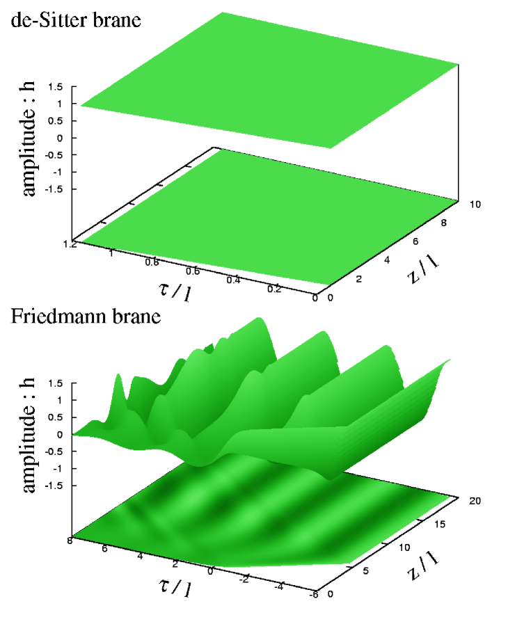
Figure 1: The evolution of a GW in the bulk. The upper panel shows the case of a de Sitter brane, while the lower panel is the case of a Friedmann brane. In both panels, we set the comoving wave number to $k=\sqrt{3}/\ell$ or $\epsilon_{*}=1.0$ with $s_{0}=100$.

Let us first consider the initial condition after inflation and check the validity of the assumption $h(t_{0},\xi)=\text{const.}$ for long-wavelength GWs. For this purpose, we plot the time evolution of GWs in the Poincaré coordinate system in Figure 1. The upper panel shows the case of the de Sitter brane by setting the equation of state on the brane to $w=-1$. The lower panel shows the case of the radiation-dominated Friedmann brane $(w=1/3)$. In both panels, we set the comoving wave number to $k=\sqrt{3}/\ell$ or $\epsilon_{*}=1.0$ with $s_{0}=100$.

In the upper panel of Figure 1, the universe on the brane experiences accelerated cosmic expansion and the wavelength of GWs becomes longer than the Hubble horizon. The resultant GW amplitude remains constant not only on the brane but also in the bulk. On the other hand, in the case of the Friedmann brane (lower), the wavelength of GW becomes shorter than the Hubble horizon at $\tau\approx-1$. In the bulk, a complicated oscillatory behavior of perturbations was found in the region that is causally connected to the physical brane. This indicates that the excitation of KK-modes occurs even if the wavelength of GWs is still outside the Hubble horizon.

These results are somewhat surprising from the viewpoint of the AdS₅ bulk, because the different behaviors simply arise from the difference in the motion of the brane. While the trajectory of the brane is described by a straight line ($d^{2}z_{\rm b}/d\tau^{2}=0$) in the case of the de Sitter brane, the trajectory of the Friedmann brane describes an arc with a non-zero curvature $d^{2}z_{\rm b}/d\tau^{2}<0$. The situation might be very similar to the moving mirror problem in an electromagnetic field (e.g., Chap. 4.4 of Ref. [19]), where the acceleration or deceleration of the mirror yields the creation of photons due to vacuum polarization. In our present case, the excitation of the KK-modes arises due to the deceleration of the moving brane.

The results in Figure 1 suggest that the initial condition $h(t_{0},\xi)=\text{const.}$ may be validated if we set the initial condition just after the end of inflation. However, the constancy of the long-wavelength mode would not be guaranteed in the case of the radiation dominated epoch, as discussed in section 2.2. This implies that the choice of the initial time $t_{0}$ is crucial when setting the initial condition at the radiation dominant epoch. Thus, for quantitative investigation of the GWs generated during inflation, the sensitivity to the choice of the initial time should be examined.

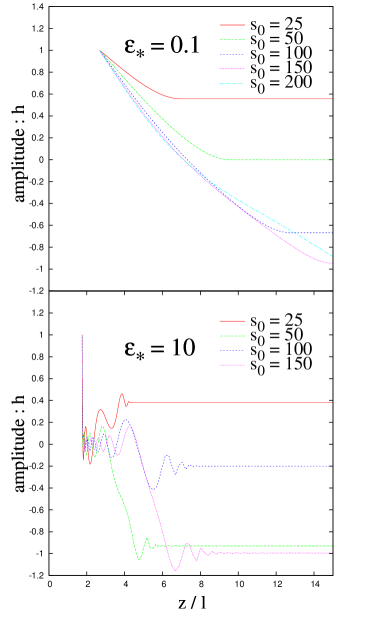
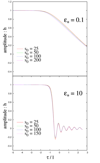
Figure 2: Left: Snapshots of the GW amplitudes in the bulk for various choices of initial time. The snapshots were taken when the wavelength of GWs becomes five times longer than the Hubble horizon, i.e., $a_{0}H/k=5$. Right: Evolved results of GWs projected on the brane starting with the various initial times.

In Figure 2, the dependence of the evolution of GWs on the initial time is plotted by varying the parameter $s_{0}$. Left panels show the snapshots of the amplitude $h(\tau,z)$ in the bulk when the wavelength of GWs just becomes five times larger than the Hubble horizon, i.e., $a_{0}H/k=5$. On the other hand, right panels show the time evolution of GWs projected on the brane. Clearly, in the bulk, the amplitude of GWs is very sensitive to the choice of the parameter $s_{0}$, or equivalently, the initial time $t_{0}$. The resultant wave form away from the physical brane does not show any convergence even in the low-energy case $(\epsilon_{*}=0.1)$. By contrast, on the brane, the GW amplitudes tend to converge if we set the initial time $t_{0}$ early enough (or set $s_{0}$ large enough).

Although we do not fully understand the reason for this convergence, as far as the GWs on the brane are concerned, the evolution of GW amplitudes becomes insensitive to the choice of the initial time when setting the parameter $s_{0}$ large enough, $s_{0}\gtrsim 50$, for instance.

3.2 Influence of high-energy effects on spectrum of gravitational wave background

Having validated the setup of the initial conditions, we now attempt to clarify the high-energy effects of the GWs and evaluate the spectrum of the SBGW on the brane. To quantify these, we wish to discriminate the influence of KK-mode excitation in the bulk from the non-standard cosmological expansion caused by the $\rho^{2}$-term in the Friedmann equation (6). For this purpose, we introduce the reference wave $h_{\rm ref}$, which is a solution of the four-dimensional wave equation just replacing the scale factor and the Hubble parameter defined in the standard Friedmann equation with those defined in the modified Friedmann equation (Eqs. (6) and (8)):

$$\ddot{h}_{\rm ref}+3H\dot{h}_{\rm ref}+\left(\frac{k}{a_{0}}\right)^{2}h_{\rm ref}=0.$$ (15)

Comparing the numerical simulations with the solution of the wave equation (15), the effect of the excitation of KK-modes can be quantified.

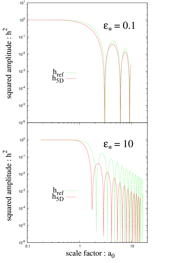
Figure 3: Squared amplitude of GWs on the brane in low-energy (upper) and the high-enery (lower) regimes. In both panels, solid lines represent the numerical solutions of wave equation (9). The dashed lines are the amplitudes of reference wave $h_{\rm ref}$ obtained from equation (15).

Figure 3 shows the squared amplitude of the GWs, $h_{\rm 5D}^{2}$ and $h_{\rm ref}^{2}$ as functions of the scale factor $a_{0}$. The upper panel shows the low-energy case ($\epsilon_{*}=0.1$), while the lower panel depicts the result in the high-energy regime ($\epsilon_{*}=10$). In both panels, the horizon re-entry time is set to $a_{0}=1$. As we increase the energy scale at horizon crossing time, the GW amplitude $h_{\rm 5D}$ becomes significantly reduced compared to the reference wave, $h_{\rm ref}$. Since the late-time evolution of GWs simply scales as $h\propto 1/a_{0}$ in both $h_{\rm 5D}$ and $h_{\rm ref}$, the results may be interpreted as the excitation of KK-modes during horizon re-entry, which are caused by an escape of five-dimensional graviton from the brane to the bulk. Note that the normalized energy density at horizon re-entry time, $\epsilon_{*}$ is related to the observed proper frequency $2\pi\,f=k/a_{0}(t_{\rm today})$ as

$$\frac{f}{f_{\text{crit}}}=\left(\frac{\sqrt{2}-1}{\epsilon_{*}}\right)^{1/4}(\ell H_{*})^{1/2}=\left(\frac{\sqrt{2}-1}{\epsilon_{*}}\right)^{1/4}(\epsilon_{*}^{2}+2\epsilon_{*})^{1/4},$$ (16)

where the critical frequency $f_{\text{crit}}$ is defined by $\ell H_{*}=1$ or $\epsilon_{*}=\sqrt{2}-1$, which typically yields $f_{\rm crit}=0.2$mHz$\,(0.1{\rm mm}/\ell)^{1/2}$ [4]. Thus, one expects from Figure 3 that the deviation from the standard four-dimensional prediction for the spectrum of SBGW becomes more prominent above the critical frequency, $f>f_{\rm crit}$.

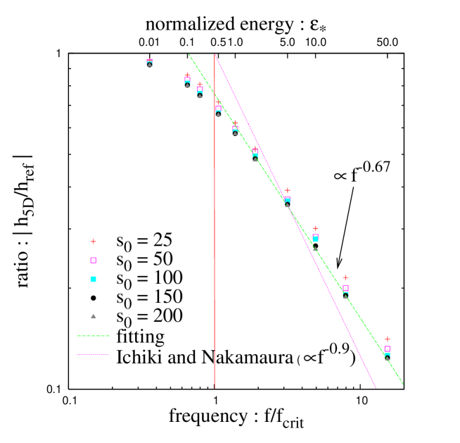
Figure 4: Frequency dependence of the ratio of amplitudes $|h_{\rm 5D}/h_{\rm ref}|$ between the numerical simulation of wave equation (9) and the reference wave (15). The vertical solid line represents the critical frequency. The dashed line indicates the fitting result (17), where fitting was examined using the data with $s_{0}=200$ at the asymptotic region $\epsilon_{*}\geq 5$. The dotted line shows the result by Ichiki and Nakamura [9].

In order to estimate the influence of KK-mode excitation on the spectrum of SBGW, the frequency dependence of the GW amplitudes is examined based on the results in Figure 3. Figure 4 shows the ratio of the amplitudes $|h_{\rm 5D}/h_{\rm ref}|$ as a result of the KK-mode excitation. The ratio is evaluated at the low-energy regime long after the horizon crossing time and is plotted as a function of the frequency $f/f_{\rm crit}$. As a reference, we also show the convergence properties of the ratio $|h_{\rm 5D}/h_{\rm ref}|$ by varying the initial time; $s_{0}=25,\,50,\,100,\,150$ and $200$. Clearly, the ratio $|h_{\rm 5D}/h_{\rm ref}|$ monotonically decreases with the frequency and the suppression of amplitude $h_{\rm 5D}$ becomes significant above the critical frequency $f_{\rm crit}$ (vertical solid line). Using the data points in the asymptotic region $\epsilon_{*}\geq 5$ (or $H_{*}\ell\geq\sqrt{35}$), we try to fit the ratio of amplitudes with $s_{0}=200$ to a power-law function. The result based on the least-square method becomes

$$\left|\frac{h_{\rm 5D}}{h_{\rm ref}}\right|=\alpha\left(\frac{f}{f_{\text{crit}}}\right)^{-\beta}$$ (17)

with $\alpha=0.76\pm 0.01$ and $\beta=0.67\pm 0.01$, which is shown as a dashed line in Figure 4.

The power-law fit (17) can be immediately translated to the spectrum of SBGW as follows. To evaluate the spectrum, we conventionally use the density parameter of SBGW $\Omega_{\rm\scriptscriptstyle GW}(f)$ defined by [20] :

$$\Omega_{\rm\scriptscriptstyle GW}(f)\equiv\frac{1}{\rho_{c}}\frac{d\rho_{\rm\scriptscriptstyle GW}}{d\log f}\propto f^{2}h^{2},$$ (18)

where $\rho_{\rm\scriptscriptstyle GW}$ is the energy density of SBGW and $\rho_{c}$ is the critical density. Above the critical frequency $f>f_{\rm crit}$, the cosmological expansion at horizon re-entry time is dominated by the $\rho^{2}$-term in the Friedmann equation (6) and we have $H_{*}\propto a_{*}^{-4}$. For the reference wave $h_{\rm ref}$, this gives $h_{\rm ref}\propto a_{*}/a_{0}\propto f^{-1/3}$, because of the relation $2\pi f\propto k\,\propto\,a_{*}H_{*}$. Thus, substituting this into the expression (18), the blue spectrum $\Omega_{\rm\scriptscriptstyle GW}\,\propto\,f^{4/3}$ is obtained if we neglect the excitation of KK-modes. Consequently, from (17), if we combine the effects of the KK-mode excitation, the SBGW spectrum becomes nearly flat, i.e.,

$$\Omega_{\rm\scriptscriptstyle GW}\,\propto\,f^{0},$$ (19)

above the critical frequency. This result seems almost indistinguishable from the standard four-dimensional prediction and slightly contradicts with the result by Ichiki and Nakamura [9], who predict a relatively steeper spetrum, $\Omega_{\rm\scriptscriptstyle GW}\,\propto\,f^{-0.46}$ from the numerical simulation based on a null coordinate system. At present, the reason for this discrepancy is unclear, however, it might be ascribed to the differences of initial conditions arising from the different choices of the bulk coordinates. Although it is premature to discuss the detectability of the SBGW, the significance of KK-mode excitations should play an important clue to probe the signature of extra-dimensions.

4 Summary and Discussion

We numerically studied the behavior of GWs in the high-energy regime of the universe in the Randall-Sundrum brane-world model. In contrast to the previous study in the GN coordinates, we used the Poincaré coordinate system in which the brane is moving in the AdS₅ background. We numerically investigated the evolution of GWs in the radiation dominated universe.

We have confirmed that the constant mode, $h(z,\tau)=$const., in the Poincaré coordinates just after inflation is a plausible initial condition from inflation. In the radiation dominated epoch, however, the constant mode does not hold in the bulk. Thus, in principle, we have to start our numerical calculations just after inflation. Fortunately, however, the resultant amplitude of the GWs on the brane becomes insensitive to the initial time $t_{0}$ of our numerical simulation if we set $t_{0}$ sufficiently early. In other words, our numerical result is insensitive to the transition time from inflation to the radiation dominated epoch if the perturbation re-enters the horizon long enough after the transition.

Based on these discussions, we turn to focus on the frequency dependence of the high-energy effects in order to predict the spectrum of SBGW. We found that the excitation of KK-modes compensates the effect of non-standard cosmological expansion. As a result, the density parameter of SBGW scales as $\Omega_{\rm\scriptscriptstyle GW}\,\propto\,f^{0}$ above the critical frequency $f_{\text{crit}}=0.2\text{mHz}\,(0.1\text{mm}/\ell)^{1/2}$. The result seems indistinguishable from the prediction in the standard four-dimensional theory and slightly contradicts with the result by Ichiki and Nakamura [9]. The most striking result of our work is that the behavior of the GWs in the bulk sensitively depends on the transition time. This feature implies that the constant initial condition in the Poincaré coordinate does not agree with the constant initial condition on the null hypersurface even on super-horizon scales. In this sense, the result obtained by Ichiki and Nakamura [9] may not necessarily agree with our results. In addition, the present numerical analysis is restricted to the frequency range $0.3\lesssim f/f_{\rm crit}\lesssim 15$. It is thus premature to discuss the detectability of the SBGW by extrapolating our numerical results to the high-frequency bands observed via future GW detectors. Nevertheless, the significance of KK-mode excitations above the critical frequency holds the clue to probe the signature of extra-dimensions and/or to constrain on brane-world models. In this respect, a more quantitative and precise prediction for the spectrum of SBGW should deserve a further investigation.

Recently, Kobayashi and Tanaka [21] analytically estimated the effect of KK-mode excitation at low-energy scales. According to their result, the amplitude of the GWs on the brane depends on the transition time as well as the energy scale $\epsilon_{*}$. This would not be a contradiction with the present numerical result because we set the initial condition in the high-energy regime $H\ell>1$, where the low-energy approximation used by the authors does not work. Thus, in order to understand our result, we need an analytical study of the KK-mode excitation in the high-energy regime. This is a challenging future work.

References

- [1] L.Randall and R.Sundrum, An alternative to compactification, Phys. Rev. Lett. 83 (1999) 4690–4693 [hep-th/9906064].
- [2] R.Maartens, Brane world gravity, Living Rev. Rel. 7 (2004) 1–99 [gr-qc/0312059].
- [3] J.Chiaverini, S.J.Smullin, A.A.Geraci, D.M.Weld and A.Kapitulnik, New experimental constraints on Non-Newtonian Forces below m, Phys. Rev. Lett. 90 (2003) 151101 [hep-ph/0209325].
- [4] C.J.Hogan, Scales of the extra dimensions and their gravitational wave backgrounds, Phys. Rev. D62 (2000) 121302(R) [astro-ph/0009136]
- [5] R.Easther, D.Langlois, R.Maartens and D.Wands, Evolution of gravitational waves in Randall-Sundrum cosmology, JCAP 10 (2003) 014 [hep-th/0308078].
- [6] R.A.Battye, C. van de Bruck, A.Mennim, Cosmological tensor perturbations in the Randall-Sundrum model: evolution in the near brane limit, Phys. Rev. D69 (2004) 064040 [hep-th/0308134].
- [7] T.Hiramatsu, K.Koyama and A.Taruya, Evolution of gravitational waves from inflationary brane-world: numerical study of high-energy effects, Phys. Lett. B 578 (2004) 269–275 [hep-th/0308072].
- [8] K.Ichiki and K.Nakamura, Causal Structure and Gravitational Waves in Brane World Cosmology, Phys. Rev. D 70 (2004) 064017 [hep-th/0310282].
- [9] K.Ichiki and K.Nakamura, Stochastic Gravitational Wave Background in Brane World Cosmology, [astro-ph/0406606].
- [10] T.Tanaka, AdS / CFT correspondence in a Friedmann-Lemaitre-Robertson-Walker brane, [gr-qc/0402068].
- [11] K.Koyama, Late time behavior of cosmological perturbations in a single brane model, JCAP 08 (2004) 012 [astro-ph/0407263].
- [12] R.A.Battye, A.Mennim, Multiple-scales analysis of cosmological perturbations in brane-worlds, [hep-th/0408101].
- [13] D.S.Gorbunov, V.A.Rubakov and S.M.Sibiryakov, Gravity waves from inflating brane or mirrors moving in AdS5, J. High. Energy Phys. 10 (2001) 015 [hep-th/0108017].
- [14] T.Kobayashi, H.Kudoh and T.Tanaka, Primordial gravitational waves in inflationary braneworld, Phys. Rev.D68 (2003) 044025 [gr-qc/0305006].
- [15] P.Kraus, Dynamics of anti-de Sitter domain walls, J. High. Energy Phys. 12 (1999) 011 [hep-th/9910149].
- [16] D.Langlois, R.Maatens and D.Wands, Gravitational waves from inflation on the brane, Phys. Lett. B489 (2000) 259–267 [hep-th/0006007].
- [17] P.Binétruy, C.Deffayet, U.Ellwanger and D.Langlois, Brane cosmological evolution in a bulk with cosmological constant, Phys. Lett. B477 (2000) 285–291 [hep-th/9910219].
- [18] C.Canuto, M.Y.Hussaini, A.Quarteroni and T.A.Zang, Spectral Methods in Fluid Dynamics, Springer Verlag (Berlin and New York), 1988.
- [19] N.D.Birrele and P.C.W.Davies, Quantum fields in curved space, Cambridge, 1982.
- [20] M.Maggiore, Gravitational wave experiments and early universe cosmology, Phys. Rep. 331 (2000) 283–367 [gr-qc/9909001].
- [21] T.Kobayashi and T.Tanaka, Leading order corrections to the cosmological evolution of tensor perturbations in braneworld, [gr-qc/0408021].