Giant Graviton Correlators from Dual $SU(N)$ super Yang-Mills Theory

Abstract:

Certain correlation functions are computed exactly in the zero coupling limit of ${\cal N}=4$ super Yang-Mills theory with gauge group $SU(N)$. A set of linearly independent operators that are in one-to-one correspondence with the half-BPS representations of the $SU(N)$ gauge theory is given. These results are used to study giant gravitons in the dual $AdS_{5}\times S^{5}$ string theory. In addition, for the $U(N)$ gauge theory, we explain how to systematically identify contributions coming from the boundary degrees of freedom.

1 Introduction

Non-perturbative string theory can now be studied, thanks to the AdS/CFT correspondence, using techniques in the dual conformal field theory[1]. It was in this spirit that giant graviton correlators were studied in [2],[3]. By studying the zero coupling limit of ${\cal N}=4$ super Yang-Mills theory with gauge group $U(N)$, candidate operators dual to giant gravitons were proposed. Further, a powerful machinery allowing the exact computation of a class of correlators at finite $N$ was developed.

In this article we take the first steps towards providing a dictionary between half-BPS representations in the ${\cal N}=4$ super Yang-Mills theory with gauge group $SU(N)$ and states in the dual supergravity. For this purpose, it is enough to study the zero coupling limit of the Yang-Mills theory. Our goal was to provide a one-to-one correspondence between the half-BPS representations and a set of operators that have diagonal two point functions. These operators (or ones related to them by a unitary transformation acting on the space of normalized operators and hence preserving the two point functions) would then be natural candidates for particle states in the supergravity. We have been partially successful.

We will now explain our interest in the extension to gauge group $SU(N)$. A $U(N)$ gauge theory is equivalent to a free $U(1)$ vector multiplet times an $SU(N)$ gauge theory up to some $Z_{N}$ identifications. The $U(1)$ vector multiplet is related to the centre of mass motion of all the branes[4]. These modes live at the boundary and are called singletons or doubletons[5]. Therefore, the bulk $AdS$ theory (in which we are interested) is describing the $SU(N)$ part of the gauge theory[6]. One of the things which interests us is the extent to which the bulk and boundary degrees of freedom can be separated in the dual super Yang-Mills theory.

One may have expected that the generalization from gauge group $U(N)$ to $SU(N)$ would imply relatively minor modification of the results of [2]. This is not the case as we now explain. In the $U(N)$ case, the space of Schur polynomials can be mapped to the space of half-BPS representations. Further, the Schur polynomials diagonalise the two point function. In the $SU(N)$ case, the number of Schur polynomials is not even equal to the number of half-BPS representations. The Schur polynomials are no longer orthogonal - in fact, they are not even linearly independent. Despite this, using the results of [2], we show that they are still a useful set of operators to consider. Indeed, by studying Schur polynomials, we are able to generalize many of the results of [2] to the $SU(N)$ case. We are also able to select a set of linearly independent operators that are in one-to-one correspondence with the half-BPS representations of the $SU(N)$ gauge theory.

Our article is organized as follows: In section 2 we give a brief review of the relevant results from [2]. In section 3 we develop the technology needed to study correlation functions in the $SU(N)$ gauge theory. In section 4 we use these results to study giant gravitons in the $AdS_{5}\times S^{5}$ string theory.

2 Review of $U(N)$ Technology

Corley, Jevicki and Ramgoolam have developed a powerful machinery for the exact computation of a class of correlators in the zero coupling limit of ${\cal N}=4$ super Yang-Mills theory with gauge group $U(N)$[2]. The operators considered in [2] are half-BPS chiral primary operators built from a single complex combination (denoted $\Phi$ in what follows) of any two of the six Higgs fields appearing in the theory. Using a total of $n$ $\Phi$s, there is a distinct operator for each partition of $n$. Further, there is a one-to-one correspondence between these operators and half-BPS representations of ${\cal R}$ charge $n$. The Schur Polynomials of degree $n$ provide a useful basis in this space of operators[2]. Indeed, in the next section we will summarize exact results obtained in [2] for the correlation functions of Schur Polynomials. We then recall the application of these results to the physics of giant gravitons. Finally, we review Berenstein’s argument [7] which essentially explains why Schur polynomials behave as D-branes.

2.1 Exact Correlators

All correlators are computed using the free field contraction

$$\langle\Phi_{ij}(x)\Phi^{*}_{kl}(y)\rangle={\delta_{ik}\delta_{jl}\over(x-y)^{2}}.$$ (1)

Consider a representation $R$ labelled by a specific Young diagram containing $n_{R}$ boxes. This Young diagram labels both a representation of $U(N)$ and a representation of $S_{n_{R}}$. Schur polynomials

$$\chi_{R}(\Phi)={1\over n!}\sum_{\sigma\in S_{n}}\chi_{R}(\sigma)\mbox{Tr\,}(\sigma\Phi),$$

where

$$\mbox{Tr\,}(\sigma\Phi)\equiv\sum_{i_{1},i_{2},\cdots i_{n}}\Phi^{i_{1}}_{i_{\sigma(1)}}\Phi^{i_{2}}_{i_{\sigma(2)}}\cdots\Phi^{i_{n}}_{i_{\sigma(n)}},$$

have a particularly simple two point correlation function

$${\langle\chi_{R}(\Phi(x))\chi_{S}(\Phi^{*}(y))\rangle=\delta_{RS}{D_{R}n_{R}!\over d_{R}}{1\over(x-y)^{n_{R}}}.}$$ (2)

In this last formula, $D_{R}$ is the dimension of the representation $R$ of the unitary group and $d_{R}$ is the dimension of representation $R$ of the permutation group. The fact that the two point function is diagonal is significant as explained below. The spacetime dependence in (2) is trivial. The non-trivial part of the result is contained in the factor obtained from the sum over $U(N)$ indices. For this reason, from now on, we suppress the spacetime dependence in all formulas. There is an equally elegant result for three point correlators: they are directly related to fusion coefficients. For a derivation of these results and further results for higher point functions, the interested reader is referred to [2].

A comment is in order: the Schur polynomials are the characters of the unitary group in their irreducible representations. The complex matrix $\Phi=\phi_{1}+i\phi_{2}$ with $\phi_{1}$ and $\phi_{2}$ $u(N)$ valued. Thus, we are considering an extension of the Schur polynomials from unitary matrices to complex matrices. These polynomials form a basis for the $U(N)$ invariant functions of $\Phi$, with $\Phi$ transforming in the adjoint representation.

2.2 Giant Gravitons

Traces involving $n<\!\!<N$ $\Phi$ fields do not mix in the large $N$ limit. Indeed, normalizing our operators so that the leading contribution to the two point function is independent of $N$ we have

$$\langle{\mbox{Tr\,}(\Phi^{n})\over N^{n\over 2}}{\mbox{Tr\,}(\Phi^{*n})\over N^{n\over 2}}\rangle=n(1+O(N^{-2})).$$

With this normalization

$$\langle{\mbox{Tr\,}(\Phi^{n_{1}})\over N^{n_{1}\over 2}}{\mbox{Tr\,}(\Phi^{n_{2}-n_{1}})\over N^{n_{2}-n_{1}\over 2}}{\mbox{Tr\,}(\Phi^{*n_{2}})\over N^{n_{2}\over 2}}\rangle=0+O({1\over N}).$$

These operators correspond to Kaluza-Klein states via the AdS/CFT correspondence. Multi-trace operators would correspond to multi-particle states, with the number of traces in the gauge theory operator matching the number of particles in the supergravity state. As $n$ increases, mixing between operators is no longer suppressed and the dictionary between single traces and single particle states is modified. To correct the dictionary, one needs to find linear combinations of operators that again do not mix. These are the operators that will have a particle interpretation in the supergravity. Since the two point function of the Schur polynomials is diagonal, they provide a natural candidate.

To provide a more detailed interpretation for the Schur polynomials, recall that in background fields, branes can get polarized into higher branes[8]. Using this insight, giant gravitons were discovered in [9] as solutions to the equations of motion following from brane actions. The giant graviton solutions describe branes extended in the sphere of the $AdS\times S$ background. These are the so-called sphere giants. The larger the angular momentum of the graviton, the larger the sphere giant. The size of these branes is limited by the radius of the sphere, thereby providing a natural cut-off on the angular momentum of gravitons in this background. In addition to these sphere giants, giant gravitons extended in the AdS space, AdS giants, were also discovered[10]. In contrast to the sphere giants, the angular momentum of the AdS giants is not cut off.

Using techniques in the dual conformal field theory, finite $N$ truncations in BPS spectra were studied as evidence of a stringy exclusion principle[11]. This stringy exclusion principle can be interpreted as evidence for non-commutative gravity [12]. The above cut-off on the angular momentum of sphere giants seems to provide a simple explanation of the stringy exclusion principle. However, the fact that the angular momentum of AdS giants is not cut off obscures this connection. Giant gravitons probably do explain the stringy exclusion principle, since there is some evidence that AdS giants with angular momentum exceeding the stringy exclusion principle bound are not BPS[13].

The number of boxes in the totally antisymmetric representation of $U(N)$ is cut off at $N$, whilst the number of boxes in the totally symmetric representation is not cut off. This has a natural physical interpretation as we now explain. The number of boxes in the Young diagram is equal to the degree of the corresponding Schur polynomial, and hence to the ${\cal R}$ charge of the operator. According to the AdS/CFT correspondence, the ${\cal R}$ charge of the super Yang-Mills operator maps into the angular momentum of the dual supergravity state. This naturally suggests[2] that the Schur polynomial for the totally antisymmetric representation is dual to a sphere giant, whilst the Schur polynomial for the totally symmetric representation is dual to an AdS giant. Convincing support for this conjecture is that these states have a well defined $1/N$ expansion and can accommodate a spectrum of open strings[14]. A Schur polynomial corresponding to a more general representation would correspond to a composite state involving giants and Kaluza-Klein gravitons.

2.3 The Schur Polynomial/D-brane Correspondence

In [7] the large $N$ gauged quantum mechanics for a single Hermitian matrix with quadratic potential was connected with a decoupling limit of ${\cal N}=4$ super Yang-Mills theory. This correspondence is very similar to the one exhibited in [15]. Three (a priori) distinct descriptions of the spectrum of the model were given. The first description employing single trace operators is naturally related to closed string states in the dual gravitational theory. The second description involves integrating the angular degrees of freedom out, so that a description in terms of eigenvalues is obtained. The integration introduces the square of the Van der Monde determinant, which is conveniently accounted for by a similarity transform after which the eigenvalues become $N$ free fermions in the harmonic oscillator potential[16]. Recently the proposal of [7] was used to provide a beautiful map between states of the Fermi theory and IIB supergravity geometries[18]. The third description of the spectrum, using the results of [2], employs a Schur polynomial basis. A surprising result of [7] is that the eigenvalue and Schur polynomial descriptions coincide!

This correspondence between the Schur polynomial description of the spectrum and the eigenvalue description essentially explains the correspondence between sphere giants and Schur polynomials corresponding to the totally antisymmetric representation and AdS giants and Schur polynomials corresponding to the totally symmetric representation. Using the map between Schur polynomials and the free fermion (i.e. eigenvalue) descriptions[7],[21] we know that the totally symmetric representation corresponds to taking the top most eigenvalue of the Fermi sea and giving it a large energy $n$ and that the totally symmetric representation corresponds to creating a hole deep in the Fermi sea. In the $c=1$ matrix model[22], these single eigenvalue excitations correspond to D-brane states. The above correspondence makes it clear that the giant graviton operators proposed in [2] are also describing the dynamics of a single eigenvalue, thereby explaining why these particular Schur polynomials are dual to D-branes.

3 Technology for $SU(N)$

In this section we use the results of [2] to develop techniques which allow an efficient computation of correlation functions of Schur polynomials $\chi_{R}(\Psi)$ with $\Psi=\phi_{1}+i\phi_{2}$ for any two ($\phi_{1},\phi_{2}\in su(N)$) of the six Higgs fields appearing in the theory. We will also give an algorithm which allows the construction of a complete basis in the space of gauge invariant operators constructed by taking traces of the $\Psi$s. This represents the required generalization of the results obtained in [2]. For complementary results relevant for the $SU(N)$ case, the reader is referred to section 10 of [3]. The method used in our work is a completely different approach. Where our results overlap, we have checked that they agree. To simplify the notation in what follows we use $\Phi=\phi_{1}+i\phi_{2}$ if $\phi_{1},\phi_{2}$ are $u(N)$ valued and $\Psi=\phi_{1}+i\phi_{2}$ if $\phi_{1},\phi_{2}$ are $su(N)$ valued.

3.1 A First Look

The essential difference between the situation considered in [2] and the situation considered in this work, is that our $\Psi$ field is traceless. This has far reaching consequences. To illustrate this point, consider the Schur polynomials built using two $\Psi$s. There are two possible representations:               and            . The Schur polynomials corresponding to these two representations are given by

$$\chi_{\hbox{}{\vbox{\offinterlineskip\vbox{\hrule height=0.3pt\hbox{\vrule height=1.435pt,width=0.3pt,depth=0.95665pt\hbox to4.78333pt{\hfil}\vrule height=1.435pt,width=0.3pt,depth=0.95665pt} \hrule height=0.3pt}\vspace{-\y@linethick} \vbox{\hrule height=0.3pt\hbox{\vrule height=1.435pt,width=0.3pt,depth=0.95665pt\hbox to4.78333pt{\hfil}\vrule height=1.435pt,width=0.3pt,depth=0.95665pt} \hrule height=0.3pt}\vspace{-\y@linethick} }}}={1\over 2}\left((\mbox{Tr\,}\Psi)^{2}-\mbox{Tr\,}(\Psi^{2})\right),\qquad\chi_{\hbox{}{\vbox{\offinterlineskip\vbox{\hrule height=0.3pt\hbox{\vrule height=1.435pt,width=0.3pt,depth=0.95665pt\hbox to4.78333pt{\hfil}\vrule height=1.435pt,width=0.3pt,depth=0.95665pt\hbox to4.78333pt{\hfil}\vrule height=1.435pt,width=0.3pt,depth=0.95665pt} \hrule height=0.3pt}\vspace{-\y@linethick} }}}={1\over 2}\left((\mbox{Tr\,}\Psi)^{2}+\mbox{Tr\,}(\Psi^{2})\right).$$

Evaluating these Schur polynomials on the (traceless) $\Psi$ field gives

$$\chi_{\hbox{}{\vbox{\offinterlineskip\vbox{\hrule height=0.3pt\hbox{\vrule height=1.435pt,width=0.3pt,depth=0.95665pt\hbox to4.78333pt{\hfil}\vrule height=1.435pt,width=0.3pt,depth=0.95665pt} \hrule height=0.3pt}\vspace{-\y@linethick} \vbox{\hrule height=0.3pt\hbox{\vrule height=1.435pt,width=0.3pt,depth=0.95665pt\hbox to4.78333pt{\hfil}\vrule height=1.435pt,width=0.3pt,depth=0.95665pt} \hrule height=0.3pt}\vspace{-\y@linethick} }}}=-\chi_{\hbox{}{\vbox{\offinterlineskip\vbox{\hrule height=0.3pt\hbox{\vrule height=1.435pt,width=0.3pt,depth=0.95665pt\hbox to4.78333pt{\hfil}\vrule height=1.435pt,width=0.3pt,depth=0.95665pt\hbox to4.78333pt{\hfil}\vrule height=1.435pt,width=0.3pt,depth=0.95665pt} \hrule height=0.3pt}\vspace{-\y@linethick} }}}\,\,.$$

This example clearly demonstrates that Schur polynomials corresponding to different representations are no longer orthogonal (or even linearly independent). The Schur polynomials are not in a one-to-one correspondence with the space of half-BPS representations and the two point function is no longer diagonal. In the remainder of this section we will argue that it is still useful to consider correlation functions of the $\chi_{R}(\Psi)$.

3.2 Recycling $U(N)$ Results

The contraction (1) for two $\Phi$ fields is to be replaced by (spacetime dependence suppressed)

$$\langle\Psi_{ij}(x)\Psi^{*}_{kl}(y)\rangle=\delta_{ik}\delta_{jl}-{1\over N}\delta_{ij}\delta_{kl}.$$ (3)

One way to interpret the above formula, is that the second term implements the tracelessness of $\Psi$ by subtracting the contribution coming from the mode associated with the trace. We could also perform this subtraction with the help of a ghost field $c$ with contractions

$$\langle cc\rangle=0=\langle c^{*}c^{*}\rangle,\qquad\langle cc^{*}\rangle=-{1\over N}=\langle c^{*}c\rangle.$$

Concretely, we have the identity

$$\langle F(\Psi_{ij},\Psi^{*}_{kl})\rangle=\langle F(\Phi_{ij}+c\delta_{ij},\Phi^{*}_{kl}+c^{*}\delta_{kl})\rangle,$$

where $F(\cdot,\cdot)$ is an arbitrary function. The advantage of trading $\Psi$ for $\Phi+c$ follows as a consequence of a particularly simple expansion of the Schur polynomial $\chi_{R}(\Phi+c)$ as a series in $c$. The coefficients in this expansion are themselves Schur polynomials in $\Phi$ so that the results of [2] can again be used, providing an efficient computational tool.

Consider a representation $R$ with $n_{R}$ boxes. The expansion we wish to develop takes the form

$$\chi_{R}(\Psi_{ij})\to\chi_{R}(\Phi_{ij}+\delta_{ij}c)=\sum_{m=0}^{n_{R}}{c^{m}\over m!}D^{m}\chi_{R}(\Phi_{ij}),\qquad D\equiv\sum_{i=1}^{N}{\partial\over\partial\Phi_{ii}}.$$

Recall that to each box in a Young diagram we can associate a weight [23]. In terms of these weights there is a particularly simple expression for the action of $D$ on the Schur polynomial

$$D\chi_{R}(\Phi)=\sum_{S}f_{S}\chi_{S}(\Phi),$$

where the sum runs over all Young diagrams $S$ that can be obtained by removing a single box from $R$ to leave a valid Young diagram and the coefficient $f_{S}$ is the weight of the removed box. It is straightforward to verify this rule using the explicit expressions for the Schur polynomials. As an illustration of the rule, consider the example

$$D\chi_{\hbox{}{\vbox{\offinterlineskip\vbox{\hrule height=0.3pt\hbox{\vrule height=1.435pt,width=0.3pt,depth=0.95665pt\hbox to4.78333pt{\hfil}\vrule height=1.435pt,width=0.3pt,depth=0.95665pt\hbox to4.78333pt{\hfil}\vrule height=1.435pt,width=0.3pt,depth=0.95665pt\hbox to4.78333pt{\hfil}\vrule height=1.435pt,width=0.3pt,depth=0.95665pt} \hrule height=0.3pt}\vspace{-\y@linethick} \vbox{\hrule height=0.3pt\hbox{\vrule height=1.435pt,width=0.3pt,depth=0.95665pt\hbox to4.78333pt{\hfil}\vrule height=1.435pt,width=0.3pt,depth=0.95665pt\hbox to4.78333pt{\hfil}\vrule height=1.435pt,width=0.3pt,depth=0.95665pt} \hrule height=0.3pt}\vspace{-\y@linethick} \vbox{\hrule height=0.3pt\hbox{\vrule height=1.435pt,width=0.3pt,depth=0.95665pt\hbox to4.78333pt{\hfil}\vrule height=1.435pt,width=0.3pt,depth=0.95665pt} \hrule height=0.3pt}\vspace{-\y@linethick} }}}(\Phi)=(N+2)\chi_{\hbox{}{\vbox{\offinterlineskip\vbox{\hrule height=0.3pt\hbox{\vrule height=1.435pt,width=0.3pt,depth=0.95665pt\hbox to4.78333pt{\hfil}\vrule height=1.435pt,width=0.3pt,depth=0.95665pt\hbox to4.78333pt{\hfil}\vrule height=1.435pt,width=0.3pt,depth=0.95665pt} \hrule height=0.3pt}\vspace{-\y@linethick} \vbox{\hrule height=0.3pt\hbox{\vrule height=1.435pt,width=0.3pt,depth=0.95665pt\hbox to4.78333pt{\hfil}\vrule height=1.435pt,width=0.3pt,depth=0.95665pt\hbox to4.78333pt{\hfil}\vrule height=1.435pt,width=0.3pt,depth=0.95665pt} \hrule height=0.3pt}\vspace{-\y@linethick} \vbox{\hrule height=0.3pt\hbox{\vrule height=1.435pt,width=0.3pt,depth=0.95665pt\hbox to4.78333pt{\hfil}\vrule height=1.435pt,width=0.3pt,depth=0.95665pt} \hrule height=0.3pt}\vspace{-\y@linethick} }}}(\Phi)+N\chi_{\hbox{}{\vbox{\offinterlineskip\vbox{\hrule height=0.3pt\hbox{\vrule height=1.435pt,width=0.3pt,depth=0.95665pt\hbox to4.78333pt{\hfil}\vrule height=1.435pt,width=0.3pt,depth=0.95665pt\hbox to4.78333pt{\hfil}\vrule height=1.435pt,width=0.3pt,depth=0.95665pt\hbox to4.78333pt{\hfil}\vrule height=1.435pt,width=0.3pt,depth=0.95665pt} \hrule height=0.3pt}\vspace{-\y@linethick} \vbox{\hrule height=0.3pt\hbox{\vrule height=1.435pt,width=0.3pt,depth=0.95665pt\hbox to4.78333pt{\hfil}\vrule height=1.435pt,width=0.3pt,depth=0.95665pt} \hrule height=0.3pt}\vspace{-\y@linethick} \vbox{\hrule height=0.3pt\hbox{\vrule height=1.435pt,width=0.3pt,depth=0.95665pt\hbox to4.78333pt{\hfil}\vrule height=1.435pt,width=0.3pt,depth=0.95665pt} \hrule height=0.3pt}\vspace{-\y@linethick} }}}(\Phi)+(N-2)\chi_{\hbox{}{\vbox{\offinterlineskip\vbox{\hrule height=0.3pt\hbox{\vrule height=1.435pt,width=0.3pt,depth=0.95665pt\hbox to4.78333pt{\hfil}\vrule height=1.435pt,width=0.3pt,depth=0.95665pt\hbox to4.78333pt{\hfil}\vrule height=1.435pt,width=0.3pt,depth=0.95665pt\hbox to4.78333pt{\hfil}\vrule height=1.435pt,width=0.3pt,depth=0.95665pt} \hrule height=0.3pt}\vspace{-\y@linethick} \vbox{\hrule height=0.3pt\hbox{\vrule height=1.435pt,width=0.3pt,depth=0.95665pt\hbox to4.78333pt{\hfil}\vrule height=1.435pt,width=0.3pt,depth=0.95665pt\hbox to4.78333pt{\hfil}\vrule height=1.435pt,width=0.3pt,depth=0.95665pt} \hrule height=0.3pt}\vspace{-\y@linethick} }}}(\Phi).$$

The action of higher powers of $D$ is obtained by iterating this action, which provides us with all the tools we need for the expansion of $\chi_{R}(\Phi_{ij}+c\delta_{ij})$.

These results allow us to efficiently compute the correlation functions of an arbitrary $n$ point function of the Schur polynomials $\chi_{S}(\Psi)$. To illustrate this point consider the computation of

$$\langle\chi_{\hbox{}{\vbox{\offinterlineskip\vbox{\hrule height=0.3pt\hbox{\vrule height=1.435pt,width=0.3pt,depth=0.95665pt\hbox to4.78333pt{\hfil}\vrule height=1.435pt,width=0.3pt,depth=0.95665pt} \hrule height=0.3pt}\vspace{-\y@linethick} \vbox{\hrule height=0.3pt\hbox{\vrule height=1.435pt,width=0.3pt,depth=0.95665pt\hbox to4.78333pt{\hfil}\vrule height=1.435pt,width=0.3pt,depth=0.95665pt} \hrule height=0.3pt}\vspace{-\y@linethick} \vbox{\hrule height=0.3pt\hbox{\vrule height=1.435pt,width=0.3pt,depth=0.95665pt\hbox to4.78333pt{\hfil}\vrule height=1.435pt,width=0.3pt,depth=0.95665pt} \hrule height=0.3pt}\vspace{-\y@linethick} }}}(\Psi)\chi_{\hbox{}{\vbox{\offinterlineskip\vbox{\hrule height=0.3pt\hbox{\vrule height=1.435pt,width=0.3pt,depth=0.95665pt\hbox to4.78333pt{\hfil}\vrule height=1.435pt,width=0.3pt,depth=0.95665pt\hbox to4.78333pt{\hfil}\vrule height=1.435pt,width=0.3pt,depth=0.95665pt} \hrule height=0.3pt}\vspace{-\y@linethick} \vbox{\hrule height=0.3pt\hbox{\vrule height=1.435pt,width=0.3pt,depth=0.95665pt\hbox to4.78333pt{\hfil}\vrule height=1.435pt,width=0.3pt,depth=0.95665pt} \hrule height=0.3pt}\vspace{-\y@linethick} }}}(\Psi^{*})\rangle=\langle\chi_{\hbox{}{\vbox{\offinterlineskip\vbox{\hrule height=0.3pt\hbox{\vrule height=1.435pt,width=0.3pt,depth=0.95665pt\hbox to4.78333pt{\hfil}\vrule height=1.435pt,width=0.3pt,depth=0.95665pt} \hrule height=0.3pt}\vspace{-\y@linethick} \vbox{\hrule height=0.3pt\hbox{\vrule height=1.435pt,width=0.3pt,depth=0.95665pt\hbox to4.78333pt{\hfil}\vrule height=1.435pt,width=0.3pt,depth=0.95665pt} \hrule height=0.3pt}\vspace{-\y@linethick} \vbox{\hrule height=0.3pt\hbox{\vrule height=1.435pt,width=0.3pt,depth=0.95665pt\hbox to4.78333pt{\hfil}\vrule height=1.435pt,width=0.3pt,depth=0.95665pt} \hrule height=0.3pt}\vspace{-\y@linethick} }}}(\Phi+{\bf 1}c)\chi_{\hbox{}{\vbox{\offinterlineskip\vbox{\hrule height=0.3pt\hbox{\vrule height=1.435pt,width=0.3pt,depth=0.95665pt\hbox to4.78333pt{\hfil}\vrule height=1.435pt,width=0.3pt,depth=0.95665pt\hbox to4.78333pt{\hfil}\vrule height=1.435pt,width=0.3pt,depth=0.95665pt} \hrule height=0.3pt}\vspace{-\y@linethick} \vbox{\hrule height=0.3pt\hbox{\vrule height=1.435pt,width=0.3pt,depth=0.95665pt\hbox to4.78333pt{\hfil}\vrule height=1.435pt,width=0.3pt,depth=0.95665pt} \hrule height=0.3pt}\vspace{-\y@linethick} }}}(\Phi^{*}+{\bf 1}c^{*})\rangle.$$

Using the expansions

$$\chi_{\hbox{}{\vbox{\offinterlineskip\vbox{\hrule height=0.3pt\hbox{\vrule height=1.435pt,width=0.3pt,depth=0.95665pt\hbox to4.78333pt{\hfil}\vrule height=1.435pt,width=0.3pt,depth=0.95665pt} \hrule height=0.3pt}\vspace{-\y@linethick} \vbox{\hrule height=0.3pt\hbox{\vrule height=1.435pt,width=0.3pt,depth=0.95665pt\hbox to4.78333pt{\hfil}\vrule height=1.435pt,width=0.3pt,depth=0.95665pt} \hrule height=0.3pt}\vspace{-\y@linethick} \vbox{\hrule height=0.3pt\hbox{\vrule height=1.435pt,width=0.3pt,depth=0.95665pt\hbox to4.78333pt{\hfil}\vrule height=1.435pt,width=0.3pt,depth=0.95665pt} \hrule height=0.3pt}\vspace{-\y@linethick} }}}(\Phi+{\bf 1}c)=\chi_{\hbox{}{\vbox{\offinterlineskip\vbox{\hrule height=0.3pt\hbox{\vrule height=1.435pt,width=0.3pt,depth=0.95665pt\hbox to4.78333pt{\hfil}\vrule height=1.435pt,width=0.3pt,depth=0.95665pt} \hrule height=0.3pt}\vspace{-\y@linethick} \vbox{\hrule height=0.3pt\hbox{\vrule height=1.435pt,width=0.3pt,depth=0.95665pt\hbox to4.78333pt{\hfil}\vrule height=1.435pt,width=0.3pt,depth=0.95665pt} \hrule height=0.3pt}\vspace{-\y@linethick} \vbox{\hrule height=0.3pt\hbox{\vrule height=1.435pt,width=0.3pt,depth=0.95665pt\hbox to4.78333pt{\hfil}\vrule height=1.435pt,width=0.3pt,depth=0.95665pt} \hrule height=0.3pt}\vspace{-\y@linethick} }}}(\Phi)+(N-2)c\chi_{\hbox{}{\vbox{\offinterlineskip\vbox{\hrule height=0.3pt\hbox{\vrule height=1.435pt,width=0.3pt,depth=0.95665pt\hbox to4.78333pt{\hfil}\vrule height=1.435pt,width=0.3pt,depth=0.95665pt} \hrule height=0.3pt}\vspace{-\y@linethick} \vbox{\hrule height=0.3pt\hbox{\vrule height=1.435pt,width=0.3pt,depth=0.95665pt\hbox to4.78333pt{\hfil}\vrule height=1.435pt,width=0.3pt,depth=0.95665pt} \hrule height=0.3pt}\vspace{-\y@linethick} }}}(\Phi)+(N-2)(N-1){c^{2}\over 2!}\chi_{\hbox{}{\vbox{\offinterlineskip\vbox{\hrule height=0.3pt\hbox{\vrule height=1.435pt,width=0.3pt,depth=0.95665pt\hbox to4.78333pt{\hfil}\vrule height=1.435pt,width=0.3pt,depth=0.95665pt} \hrule height=0.3pt}\vspace{-\y@linethick} }}}(\Phi)+(N-2)(N-1)N{c^{3}\over 3!},$$

$$\chi_{\hbox{}{\vbox{\offinterlineskip\vbox{\hrule height=0.3pt\hbox{\vrule height=1.435pt,width=0.3pt,depth=0.95665pt\hbox to4.78333pt{\hfil}\vrule height=1.435pt,width=0.3pt,depth=0.95665pt\hbox to4.78333pt{\hfil}\vrule height=1.435pt,width=0.3pt,depth=0.95665pt} \hrule height=0.3pt}\vspace{-\y@linethick} \vbox{\hrule height=0.3pt\hbox{\vrule height=1.435pt,width=0.3pt,depth=0.95665pt\hbox to4.78333pt{\hfil}\vrule height=1.435pt,width=0.3pt,depth=0.95665pt} \hrule height=0.3pt}\vspace{-\y@linethick} }}}(\Phi^{*}+{\bf 1}c^{*})= \chi_{\hbox{}{\vbox{\offinterlineskip\vbox{\hrule height=0.3pt\hbox{\vrule height=1.435pt,width=0.3pt,depth=0.95665pt\hbox to4.78333pt{\hfil}\vrule height=1.435pt,width=0.3pt,depth=0.95665pt\hbox to4.78333pt{\hfil}\vrule height=1.435pt,width=0.3pt,depth=0.95665pt} \hrule height=0.3pt}\vspace{-\y@linethick} \vbox{\hrule height=0.3pt\hbox{\vrule height=1.435pt,width=0.3pt,depth=0.95665pt\hbox to4.78333pt{\hfil}\vrule height=1.435pt,width=0.3pt,depth=0.95665pt} \hrule height=0.3pt}\vspace{-\y@linethick} }}}(\Phi^{*})+(N+1)c^{*}\chi_{\hbox{}{\vbox{\offinterlineskip\vbox{\hrule height=0.3pt\hbox{\vrule height=1.435pt,width=0.3pt,depth=0.95665pt\hbox to4.78333pt{\hfil}\vrule height=1.435pt,width=0.3pt,depth=0.95665pt} \hrule height=0.3pt}\vspace{-\y@linethick} \vbox{\hrule height=0.3pt\hbox{\vrule height=1.435pt,width=0.3pt,depth=0.95665pt\hbox to4.78333pt{\hfil}\vrule height=1.435pt,width=0.3pt,depth=0.95665pt} \hrule height=0.3pt}\vspace{-\y@linethick} }}}(\Phi^{*})+(N-1)c^{*}\chi_{\hbox{}{\vbox{\offinterlineskip\vbox{\hrule height=0.3pt\hbox{\vrule height=1.435pt,width=0.3pt,depth=0.95665pt\hbox to4.78333pt{\hfil}\vrule height=1.435pt,width=0.3pt,depth=0.95665pt\hbox to4.78333pt{\hfil}\vrule height=1.435pt,width=0.3pt,depth=0.95665pt} \hrule height=0.3pt}\vspace{-\y@linethick} }}}(\Phi^{*})$$

$$+ 2(N^{2}-1){c^{*2}\over 2!}\chi_{\hbox{}{\vbox{\offinterlineskip\vbox{\hrule height=0.3pt\hbox{\vrule height=1.435pt,width=0.3pt,depth=0.95665pt\hbox to4.78333pt{\hfil}\vrule height=1.435pt,width=0.3pt,depth=0.95665pt} \hrule height=0.3pt}\vspace{-\y@linethick} }}}(\Phi^{*})+2N(N^{2}-1){c^{*3}\over 3!},$$

and the formula

$$\langle c^{n}c^{*m}\rangle={\delta^{mn}(-1)^{n}n!\over N^{n}},$$

we easily obtain

$$\langle\chi_{\hbox{}{\vbox{\offinterlineskip\vbox{\hrule height=0.3pt\hbox{\vrule height=1.435pt,width=0.3pt,depth=0.95665pt\hbox to4.78333pt{\hfil}\vrule height=1.435pt,width=0.3pt,depth=0.95665pt} \hrule height=0.3pt}\vspace{-\y@linethick} \vbox{\hrule height=0.3pt\hbox{\vrule height=1.435pt,width=0.3pt,depth=0.95665pt\hbox to4.78333pt{\hfil}\vrule height=1.435pt,width=0.3pt,depth=0.95665pt} \hrule height=0.3pt}\vspace{-\y@linethick} \vbox{\hrule height=0.3pt\hbox{\vrule height=1.435pt,width=0.3pt,depth=0.95665pt\hbox to4.78333pt{\hfil}\vrule height=1.435pt,width=0.3pt,depth=0.95665pt} \hrule height=0.3pt}\vspace{-\y@linethick} }}}(\Psi)\chi_{\hbox{}{\vbox{\offinterlineskip\vbox{\hrule height=0.3pt\hbox{\vrule height=1.435pt,width=0.3pt,depth=0.95665pt\hbox to4.78333pt{\hfil}\vrule height=1.435pt,width=0.3pt,depth=0.95665pt\hbox to4.78333pt{\hfil}\vrule height=1.435pt,width=0.3pt,depth=0.95665pt} \hrule height=0.3pt}\vspace{-\y@linethick} \vbox{\hrule height=0.3pt\hbox{\vrule height=1.435pt,width=0.3pt,depth=0.95665pt\hbox to4.78333pt{\hfil}\vrule height=1.435pt,width=0.3pt,depth=0.95665pt} \hrule height=0.3pt}\vspace{-\y@linethick} }}}(\Psi^{*})\rangle= \langle\chi_{\hbox{}{\vbox{\offinterlineskip\vbox{\hrule height=0.3pt\hbox{\vrule height=1.435pt,width=0.3pt,depth=0.95665pt\hbox to4.78333pt{\hfil}\vrule height=1.435pt,width=0.3pt,depth=0.95665pt} \hrule height=0.3pt}\vspace{-\y@linethick} \vbox{\hrule height=0.3pt\hbox{\vrule height=1.435pt,width=0.3pt,depth=0.95665pt\hbox to4.78333pt{\hfil}\vrule height=1.435pt,width=0.3pt,depth=0.95665pt} \hrule height=0.3pt}\vspace{-\y@linethick} \vbox{\hrule height=0.3pt\hbox{\vrule height=1.435pt,width=0.3pt,depth=0.95665pt\hbox to4.78333pt{\hfil}\vrule height=1.435pt,width=0.3pt,depth=0.95665pt} \hrule height=0.3pt}\vspace{-\y@linethick} }}}(\Phi)\chi_{\hbox{}{\vbox{\offinterlineskip\vbox{\hrule height=0.3pt\hbox{\vrule height=1.435pt,width=0.3pt,depth=0.95665pt\hbox to4.78333pt{\hfil}\vrule height=1.435pt,width=0.3pt,depth=0.95665pt\hbox to4.78333pt{\hfil}\vrule height=1.435pt,width=0.3pt,depth=0.95665pt} \hrule height=0.3pt}\vspace{-\y@linethick} \vbox{\hrule height=0.3pt\hbox{\vrule height=1.435pt,width=0.3pt,depth=0.95665pt\hbox to4.78333pt{\hfil}\vrule height=1.435pt,width=0.3pt,depth=0.95665pt} \hrule height=0.3pt}\vspace{-\y@linethick} }}}(\Phi^{*})\rangle$$

$$- {1\over N}\langle(N-2)\chi_{\hbox{}{\vbox{\offinterlineskip\vbox{\hrule height=0.3pt\hbox{\vrule height=1.435pt,width=0.3pt,depth=0.95665pt\hbox to4.78333pt{\hfil}\vrule height=1.435pt,width=0.3pt,depth=0.95665pt} \hrule height=0.3pt}\vspace{-\y@linethick} \vbox{\hrule height=0.3pt\hbox{\vrule height=1.435pt,width=0.3pt,depth=0.95665pt\hbox to4.78333pt{\hfil}\vrule height=1.435pt,width=0.3pt,depth=0.95665pt} \hrule height=0.3pt}\vspace{-\y@linethick} }}}(\Phi)\left[(N+1)\chi_{\hbox{}{\vbox{\offinterlineskip\vbox{\hrule height=0.3pt\hbox{\vrule height=1.435pt,width=0.3pt,depth=0.95665pt\hbox to4.78333pt{\hfil}\vrule height=1.435pt,width=0.3pt,depth=0.95665pt} \hrule height=0.3pt}\vspace{-\y@linethick} \vbox{\hrule height=0.3pt\hbox{\vrule height=1.435pt,width=0.3pt,depth=0.95665pt\hbox to4.78333pt{\hfil}\vrule height=1.435pt,width=0.3pt,depth=0.95665pt} \hrule height=0.3pt}\vspace{-\y@linethick} }}}(\Phi^{*})+(N-1)\chi_{\hbox{}{\vbox{\offinterlineskip\vbox{\hrule height=0.3pt\hbox{\vrule height=1.435pt,width=0.3pt,depth=0.95665pt\hbox to4.78333pt{\hfil}\vrule height=1.435pt,width=0.3pt,depth=0.95665pt\hbox to4.78333pt{\hfil}\vrule height=1.435pt,width=0.3pt,depth=0.95665pt} \hrule height=0.3pt}\vspace{-\y@linethick} }}}(\Phi^{*})\right]\rangle$$

$$+ {1\over N^{2}}\langle(N-2)(N-1)\chi_{\hbox{}{\vbox{\offinterlineskip\vbox{\hrule height=0.3pt\hbox{\vrule height=1.435pt,width=0.3pt,depth=0.95665pt\hbox to4.78333pt{\hfil}\vrule height=1.435pt,width=0.3pt,depth=0.95665pt} \hrule height=0.3pt}\vspace{-\y@linethick} }}}(\Phi)\left[(N^{2}-1)\chi_{\hbox{}{\vbox{\offinterlineskip\vbox{\hrule height=0.3pt\hbox{\vrule height=1.435pt,width=0.3pt,depth=0.95665pt\hbox to4.78333pt{\hfil}\vrule height=1.435pt,width=0.3pt,depth=0.95665pt} \hrule height=0.3pt}\vspace{-\y@linethick} }}}(\Phi^{*})\right]\rangle$$

$$- {2N^{2}(N^{2}-1)(N-2)(N-1)\over 3!N^{3}}$$

The remaining correlators can now all be evaluated using (2). The results of this section could also have been obtained without introducing the ghost $c$ and simply using the contraction (3). This is the approach taken in [3]. We have checked that our results are in complete agreement. The generalization to $n$ point functions is obvious.

3.3 Constraints

We have already seen that because $\mbox{Tr\,}(\Psi)=0$, not all Schur polynomials $\chi_{R}(\Psi)$ are linearly independent. In this section we obtain a complete set of linear relations between the $\chi_{R}(\Psi)$s. For a different use of the $\mbox{Tr\,}(\Psi)=0$ condition, consult[3].

Recall that the character for a group element $T$ in a direct product representation $\chi_{R\times S}(T)$ is equal to the product of the characters $\chi_{R}(T)\chi_{S}(T)$. The characters of the unitary group are given by the Schur polynomials. Thus, the Schur polynomials themselves obey these relations. The fact that we evaluate the Schur polynomials on the complex matrix $\Psi$ and not on a unitary matrix is of no consequence. Using this insight, we can write down expressions obtained by multiplying        with an arbitrary representation $R$. Upon noting that

$$\chi_{\hbox{}{\vbox{\offinterlineskip\vbox{\hrule height=0.3pt\hbox{\vrule height=1.435pt,width=0.3pt,depth=0.95665pt\hbox to4.78333pt{\hfil}\vrule height=1.435pt,width=0.3pt,depth=0.95665pt} \hrule height=0.3pt}\vspace{-\y@linethick} }}}(\Psi)=\mbox{Tr\,}(\Psi)=0,$$

we see that this leads to a set of constraints obeyed by the $\chi_{R}(\Psi)$. As an example

$$\chi_{\hbox{}{\vbox{\offinterlineskip\vbox{\hrule height=0.3pt\hbox{\vrule height=1.435pt,width=0.3pt,depth=0.95665pt\hbox to4.78333pt{\hfil}\vrule height=1.435pt,width=0.3pt,depth=0.95665pt} \hrule height=0.3pt}\vspace{-\y@linethick} }}}(\Psi)\chi_{\hbox{}{\vbox{\offinterlineskip\vbox{\hrule height=0.3pt\hbox{\vrule height=1.435pt,width=0.3pt,depth=0.95665pt\hbox to4.78333pt{\hfil}\vrule height=1.435pt,width=0.3pt,depth=0.95665pt} \hrule height=0.3pt}\vspace{-\y@linethick} \vbox{\hrule height=0.3pt\hbox{\vrule height=1.435pt,width=0.3pt,depth=0.95665pt\hbox to4.78333pt{\hfil}\vrule height=1.435pt,width=0.3pt,depth=0.95665pt} \hrule height=0.3pt}\vspace{-\y@linethick} }}}(\Psi)=\chi_{\hbox{}{\vbox{\offinterlineskip\vbox{\hrule height=0.3pt\hbox{\vrule height=1.435pt,width=0.3pt,depth=0.95665pt\hbox to4.78333pt{\hfil}\vrule height=1.435pt,width=0.3pt,depth=0.95665pt} \hrule height=0.3pt}\vspace{-\y@linethick} \vbox{\hrule height=0.3pt\hbox{\vrule height=1.435pt,width=0.3pt,depth=0.95665pt\hbox to4.78333pt{\hfil}\vrule height=1.435pt,width=0.3pt,depth=0.95665pt} \hrule height=0.3pt}\vspace{-\y@linethick} \vbox{\hrule height=0.3pt\hbox{\vrule height=1.435pt,width=0.3pt,depth=0.95665pt\hbox to4.78333pt{\hfil}\vrule height=1.435pt,width=0.3pt,depth=0.95665pt} \hrule height=0.3pt}\vspace{-\y@linethick} }}}(\Psi)+\chi_{\hbox{}{\vbox{\offinterlineskip\vbox{\hrule height=0.3pt\hbox{\vrule height=1.435pt,width=0.3pt,depth=0.95665pt\hbox to4.78333pt{\hfil}\vrule height=1.435pt,width=0.3pt,depth=0.95665pt\hbox to4.78333pt{\hfil}\vrule height=1.435pt,width=0.3pt,depth=0.95665pt} \hrule height=0.3pt}\vspace{-\y@linethick} \vbox{\hrule height=0.3pt\hbox{\vrule height=1.435pt,width=0.3pt,depth=0.95665pt\hbox to4.78333pt{\hfil}\vrule height=1.435pt,width=0.3pt,depth=0.95665pt} \hrule height=0.3pt}\vspace{-\y@linethick} }}}(\Psi)=0$$

which is easily verified explicitly. The number of relations between the Schur polynomials corresponding to Young diagrams with $n$ boxes obtained using the above procedure is equal to the number of Schur polynomials corresponding to Young diagrams with $n-1$ boxes.

We will now argue that the set of relations obtained in this way is a complete set. To do this, we will be using the classification of half BPS operators given in [3]. The total number of linearly independent Schur polynomials is equal to the total number of Schur polynomials minus the number of relations between them. The number of Schur polynomials for a given number $n$ boxes is equal to the number of irreducible inequivalent representations of the permutation group $S_{n}$. This is in turn equal to the number of partitions of $n$. This can be computed by reading off the power of $x^{n}$ in the expansion of the product

$$f_{1}(x)=\prod_{m=1}^{\infty}{1\over 1-x^{m}}\equiv\sum_{n=0}^{\infty}c_{n}x^{n}.$$

The number of linearly independent polynomials built from $n$ $\Psi$s is equal to the number of partitions of $n$ which do not include any 1s in the partitions. Excluding 1s accounts for the fact that products including any factors of $\mbox{Tr\,}(\Psi)$ vanish. This can be computed by reading off the power of $x^{n}$ in the expansion of the product

$$f_{2}(x)=\prod_{m=2}^{\infty}{1\over 1-x^{m}}\equiv\sum_{n=0}^{\infty}d_{n}x^{n}.$$

Noting that $(1-x)f_{1}(x)=f_{2}(x)$, we see that

$$d_{n}=c_{n}-c_{n-1}.$$

Thus, the total number of relations between Schur polynomials corresponding to Young diagrams with $n$ boxes is equal to the number of Schur polynomials with $n-1$ boxes, which is precisely equal to the number of constraints we found above.

The local operators in ${\cal N}=4$ super Yang-Mills theory can be organized into irreducible representations of the $D=4$ ${\cal N}=4$ superconformal algebra. Each irreducible representation contains special operators of lowest scaling dimension related to their ${\cal R}$ charge, the so-called chiral primary operators. They transform in the $(0,l,0)$ representation of the $SU(4)$ ${\cal R}$ symmetry. From each of these $(0,l,0)$ representations we can select a unique state built from a product of $l$ $\Psi$s. Since the ${\cal R}$ symmetry transformation of our operator is independent of how we choose to contract the gauge indices, we can count the number of irreducible representations by counting the number of ways we have of contracting the gauge indices on $l$ $\Psi$s. This is of course equal to $d_{l}$.

3.4 A Linearly Independent Basis of $SU(N)$ BPS Operators

In this section we will use polynomials with a different normalization

$$\tilde{\chi}_{R}(\Psi)={d_{R}\over D_{R}n_{R}!}\chi_{R}(\Psi).$$

The advantage of this normalization is that the action of $D$ is now

$$D\tilde{\chi}_{R}(\Phi)=\sum_{S}\tilde{\chi}_{S}(\Phi),$$

where the sum again runs over all valid Young diagrams that can be obtained from $R$ by removing a single box. Notice that $D$ maps the space of Schur polynomials associated with Young diagrams with $n$ boxes (of dimension $c_{n}$) to the space of Schur polynomials associated with Young diagrams with $n-1$ boxes (of dimension $c_{n-1}$). Clearly, $D$ has $c_{n}-c_{n-1}=d_{n}$ zero eigenvectors. This is equal to the number of linearly independent Schur polynomials built from the $\Psi$s. Thus, the basis of the null space of $D$ is in a one-to-one correspondence with the half-BPS representations of the super Yang-Mills theory with gauge group $SU(N)$. For any null vector of $D$, $Df(\Phi)=0$ we have the identity

$$f(\Psi)\to f(\Phi+c{\bf 1})=f(\Phi).$$

This implies a significant simplification: for this class of operators all computations can be performed without making use of the ghost $c$.

In the remainder of this section we give an algorithm which provides an explicit construction of a basis for the null space of $D$. Towards this end we introduce the notion of a fixed top block Young diagram. We call the block in the first row in the right most position, the top block in the Young diagram. If the top block cannot be removed to leave a legal Young diagram, we say we have a fixed top block Young diagram. The importance of the fixed top block Young diagrams is that they can be put into a one-to-one correspondence with the null vectors of $D$. If a Young diagram is not a fixed top block diagram, it is a moveable top block diagram.

To illustrate our argument we will construct a basis for the null vectors of $D$ of ${\cal R}$ charge $n$. The full set of relations between the Schur polynomials $\chi_{R}(\Psi)$ associated with Young diagrams of $n$ boxes can be used to eliminate all of the moveable top block Young diagrams of $n$ boxes. Each relation is obtained by taking the product of the fundamental representation (        ) with a representation corresponding to a Young diagram with $n-1$ boxes. Use each such relation to eliminate the moveable top block Young diagram obtained by adding        to the Young diagram with $n-1$ boxes, so that the added box is in the top block position. Note that every moveable top block Young diagram can be obtained by adding        to a Young diagram with $n-1$ boxes, so that the added box is in the top block position. Thus, this eliminates all of the moveable top block Young diagrams.

Our algorithm constructs a null vector of $D$ from each fixed top block diagram by using an operation we call the reduction of the Schur polynomial. The reduction of a Schur polynomial is obtained by taking minus one times the sum of Schur Polynomials corresponding to diagrams that can be obtained by all moves which move a box into the first row, such that after the move we obtain a valid Young diagram. As an example, the reduction of $\chi_{\hbox{}{\vbox{\offinterlineskip\vbox{\hrule height=0.3pt\hbox{\vrule height=1.435pt,width=0.3pt,depth=0.95665pt\hbox to4.78333pt{\hfil}\vrule height=1.435pt,width=0.3pt,depth=0.95665pt\hbox to4.78333pt{\hfil}\vrule height=1.435pt,width=0.3pt,depth=0.95665pt\hbox to4.78333pt{\hfil}\vrule height=1.435pt,width=0.3pt,depth=0.95665pt} \hrule height=0.3pt}\vspace{-\y@linethick} \vbox{\hrule height=0.3pt\hbox{\vrule height=1.435pt,width=0.3pt,depth=0.95665pt\hbox to4.78333pt{\hfil}\vrule height=1.435pt,width=0.3pt,depth=0.95665pt\hbox to4.78333pt{\hfil}\vrule height=1.435pt,width=0.3pt,depth=0.95665pt} \hrule height=0.3pt}\vspace{-\y@linethick} \vbox{\hrule height=0.3pt\hbox{\vrule height=1.435pt,width=0.3pt,depth=0.95665pt\hbox to4.78333pt{\hfil}\vrule height=1.435pt,width=0.3pt,depth=0.95665pt} \hrule height=0.3pt}\vspace{-\y@linethick} }}}(\Psi)$ is given by

$$-\chi_{\hbox{}{\vbox{\offinterlineskip\vbox{\hrule height=0.3pt\hbox{\vrule height=1.435pt,width=0.3pt,depth=0.95665pt\hbox to4.78333pt{\hfil}\vrule height=1.435pt,width=0.3pt,depth=0.95665pt\hbox to4.78333pt{\hfil}\vrule height=1.435pt,width=0.3pt,depth=0.95665pt\hbox to4.78333pt{\hfil}\vrule height=1.435pt,width=0.3pt,depth=0.95665pt\hbox to4.78333pt{\hfil}\vrule height=1.435pt,width=0.3pt,depth=0.95665pt} \hrule height=0.3pt}\vspace{-\y@linethick} \vbox{\hrule height=0.3pt\hbox{\vrule height=1.435pt,width=0.3pt,depth=0.95665pt\hbox to4.78333pt{\hfil}\vrule height=1.435pt,width=0.3pt,depth=0.95665pt} \hrule height=0.3pt}\vspace{-\y@linethick} \vbox{\hrule height=0.3pt\hbox{\vrule height=1.435pt,width=0.3pt,depth=0.95665pt\hbox to4.78333pt{\hfil}\vrule height=1.435pt,width=0.3pt,depth=0.95665pt} \hrule height=0.3pt}\vspace{-\y@linethick} }}}(\Psi)-\chi_{\hbox{}{\vbox{\offinterlineskip\vbox{\hrule height=0.3pt\hbox{\vrule height=1.435pt,width=0.3pt,depth=0.95665pt\hbox to4.78333pt{\hfil}\vrule height=1.435pt,width=0.3pt,depth=0.95665pt\hbox to4.78333pt{\hfil}\vrule height=1.435pt,width=0.3pt,depth=0.95665pt\hbox to4.78333pt{\hfil}\vrule height=1.435pt,width=0.3pt,depth=0.95665pt\hbox to4.78333pt{\hfil}\vrule height=1.435pt,width=0.3pt,depth=0.95665pt} \hrule height=0.3pt}\vspace{-\y@linethick} \vbox{\hrule height=0.3pt\hbox{\vrule height=1.435pt,width=0.3pt,depth=0.95665pt\hbox to4.78333pt{\hfil}\vrule height=1.435pt,width=0.3pt,depth=0.95665pt\hbox to4.78333pt{\hfil}\vrule height=1.435pt,width=0.3pt,depth=0.95665pt} \hrule height=0.3pt}\vspace{-\y@linethick} }}}(\Psi).$$

As another example, the reduction of $\chi_{\hbox{}{\vbox{\offinterlineskip\vbox{\hrule height=0.3pt\hbox{\vrule height=1.435pt,width=0.3pt,depth=0.95665pt\hbox to4.78333pt{\hfil}\vrule height=1.435pt,width=0.3pt,depth=0.95665pt\hbox to4.78333pt{\hfil}\vrule height=1.435pt,width=0.3pt,depth=0.95665pt\hbox to4.78333pt{\hfil}\vrule height=1.435pt,width=0.3pt,depth=0.95665pt\hbox to4.78333pt{\hfil}\vrule height=1.435pt,width=0.3pt,depth=0.95665pt} \hrule height=0.3pt}\vspace{-\y@linethick} }}}(\Psi)$ is zero. We can obtain a higher order reduction by reducing a reduction of the Schur polynomial. For a Schur polynomial with $n$ boxes, we reduce at most $n$ times. We can now state our algorithm: by starting with a Schur polynomial corresponding to a fixed top block Young diagram and adding all possible reductions, we obtain a null vector of $D$.

We end this section with a construction of the null vectors of $D$ of ${\cal R}$ charge 4. There are two fixed top block Young diagrams (                             and                   ). Applying our algorithm we obtain two null vectors

$$\chi_{1}(\Psi)=\chi_{\hbox{}{\vbox{\offinterlineskip\vbox{\hrule height=0.3pt\hbox{\vrule height=1.435pt,width=0.3pt,depth=0.95665pt\hbox to4.78333pt{\hfil}\vrule height=1.435pt,width=0.3pt,depth=0.95665pt} \hrule height=0.3pt}\vspace{-\y@linethick} \vbox{\hrule height=0.3pt\hbox{\vrule height=1.435pt,width=0.3pt,depth=0.95665pt\hbox to4.78333pt{\hfil}\vrule height=1.435pt,width=0.3pt,depth=0.95665pt} \hrule height=0.3pt}\vspace{-\y@linethick} \vbox{\hrule height=0.3pt\hbox{\vrule height=1.435pt,width=0.3pt,depth=0.95665pt\hbox to4.78333pt{\hfil}\vrule height=1.435pt,width=0.3pt,depth=0.95665pt} \hrule height=0.3pt}\vspace{-\y@linethick} \vbox{\hrule height=0.3pt\hbox{\vrule height=1.435pt,width=0.3pt,depth=0.95665pt\hbox to4.78333pt{\hfil}\vrule height=1.435pt,width=0.3pt,depth=0.95665pt} \hrule height=0.3pt}\vspace{-\y@linethick} }}}(\Psi)-\chi_{\hbox{}{\vbox{\offinterlineskip\vbox{\hrule height=0.3pt\hbox{\vrule height=1.435pt,width=0.3pt,depth=0.95665pt\hbox to4.78333pt{\hfil}\vrule height=1.435pt,width=0.3pt,depth=0.95665pt\hbox to4.78333pt{\hfil}\vrule height=1.435pt,width=0.3pt,depth=0.95665pt} \hrule height=0.3pt}\vspace{-\y@linethick} \vbox{\hrule height=0.3pt\hbox{\vrule height=1.435pt,width=0.3pt,depth=0.95665pt\hbox to4.78333pt{\hfil}\vrule height=1.435pt,width=0.3pt,depth=0.95665pt} \hrule height=0.3pt}\vspace{-\y@linethick} \vbox{\hrule height=0.3pt\hbox{\vrule height=1.435pt,width=0.3pt,depth=0.95665pt\hbox to4.78333pt{\hfil}\vrule height=1.435pt,width=0.3pt,depth=0.95665pt} \hrule height=0.3pt}\vspace{-\y@linethick} }}}(\Psi)+\chi_{\hbox{}{\vbox{\offinterlineskip\vbox{\hrule height=0.3pt\hbox{\vrule height=1.435pt,width=0.3pt,depth=0.95665pt\hbox to4.78333pt{\hfil}\vrule height=1.435pt,width=0.3pt,depth=0.95665pt\hbox to4.78333pt{\hfil}\vrule height=1.435pt,width=0.3pt,depth=0.95665pt\hbox to4.78333pt{\hfil}\vrule height=1.435pt,width=0.3pt,depth=0.95665pt} \hrule height=0.3pt}\vspace{-\y@linethick} \vbox{\hrule height=0.3pt\hbox{\vrule height=1.435pt,width=0.3pt,depth=0.95665pt\hbox to4.78333pt{\hfil}\vrule height=1.435pt,width=0.3pt,depth=0.95665pt} \hrule height=0.3pt}\vspace{-\y@linethick} }}}(\Psi)-\chi_{\hbox{}{\vbox{\offinterlineskip\vbox{\hrule height=0.3pt\hbox{\vrule height=1.435pt,width=0.3pt,depth=0.95665pt\hbox to4.78333pt{\hfil}\vrule height=1.435pt,width=0.3pt,depth=0.95665pt\hbox to4.78333pt{\hfil}\vrule height=1.435pt,width=0.3pt,depth=0.95665pt\hbox to4.78333pt{\hfil}\vrule height=1.435pt,width=0.3pt,depth=0.95665pt\hbox to4.78333pt{\hfil}\vrule height=1.435pt,width=0.3pt,depth=0.95665pt} \hrule height=0.3pt}\vspace{-\y@linethick} }}}(\Psi)$$

and

$$\chi_{2}(\Psi)=\chi_{\hbox{}{\vbox{\offinterlineskip\vbox{\hrule height=0.3pt\hbox{\vrule height=1.435pt,width=0.3pt,depth=0.95665pt\hbox to4.78333pt{\hfil}\vrule height=1.435pt,width=0.3pt,depth=0.95665pt\hbox to4.78333pt{\hfil}\vrule height=1.435pt,width=0.3pt,depth=0.95665pt} \hrule height=0.3pt}\vspace{-\y@linethick} \vbox{\hrule height=0.3pt\hbox{\vrule height=1.435pt,width=0.3pt,depth=0.95665pt\hbox to4.78333pt{\hfil}\vrule height=1.435pt,width=0.3pt,depth=0.95665pt\hbox to4.78333pt{\hfil}\vrule height=1.435pt,width=0.3pt,depth=0.95665pt} \hrule height=0.3pt}\vspace{-\y@linethick} }}}(\Psi)-\chi_{\hbox{}{\vbox{\offinterlineskip\vbox{\hrule height=0.3pt\hbox{\vrule height=1.435pt,width=0.3pt,depth=0.95665pt\hbox to4.78333pt{\hfil}\vrule height=1.435pt,width=0.3pt,depth=0.95665pt\hbox to4.78333pt{\hfil}\vrule height=1.435pt,width=0.3pt,depth=0.95665pt\hbox to4.78333pt{\hfil}\vrule height=1.435pt,width=0.3pt,depth=0.95665pt} \hrule height=0.3pt}\vspace{-\y@linethick} \vbox{\hrule height=0.3pt\hbox{\vrule height=1.435pt,width=0.3pt,depth=0.95665pt\hbox to4.78333pt{\hfil}\vrule height=1.435pt,width=0.3pt,depth=0.95665pt} \hrule height=0.3pt}\vspace{-\y@linethick} }}}(\Psi)+\chi_{\hbox{}{\vbox{\offinterlineskip\vbox{\hrule height=0.3pt\hbox{\vrule height=1.435pt,width=0.3pt,depth=0.95665pt\hbox to4.78333pt{\hfil}\vrule height=1.435pt,width=0.3pt,depth=0.95665pt\hbox to4.78333pt{\hfil}\vrule height=1.435pt,width=0.3pt,depth=0.95665pt\hbox to4.78333pt{\hfil}\vrule height=1.435pt,width=0.3pt,depth=0.95665pt\hbox to4.78333pt{\hfil}\vrule height=1.435pt,width=0.3pt,depth=0.95665pt} \hrule height=0.3pt}\vspace{-\y@linethick} }}}(\Psi).$$

It is easy to check that

$$\langle\chi_{1}(\Psi)\chi_{2}(\Psi^{*})\rangle=\langle\chi_{1}(\Phi)\chi_{2}(\Phi^{*})\rangle\neq 0.$$

Thus, the basis constructed using our algorithm is not an orthogonal basis. To see that it is indeed linearly independent is easy: the question of linear dependence of these operators can be settled by computing two point functions. To compute these, we can replace all $\Psi$s by $\Phi$s, thanks to the fact that all of our operators are null vectors of $D$. Upon replacing all $\Psi$s by $\Phi$s the linear independence of the basis follows because Schur polynomials of the $\Phi$s corresponding to distinct Young diagrams are linearly independent and each fixed top block Young diagram appears in a unique operator belonging to our basis.

If the mixing between these operators was suppressed as $N\to\infty$, they would still have formed natural candidates for particle states in the classical limit of the dual quantum gravity. It is however easy to check that this mixing is not suppressed as $N\to\infty$.

3.5 Correlators of traces in the $SU(N)$ theory

Given the correlators of Schur polynomials, following [3] we can compute correlators of the form

$$\langle\mbox{Tr\,}(\sigma_{1}\Psi)\mbox{Tr\,}(\sigma_{2}\Psi)\rangle,$$

with $\sigma_{1},\sigma_{2}\in S_{n}$ for any $n$. For $n$ of order $\sim 1$ these correspond to Kaluza-Klein modes. Upon using the orthogonality of the characters of $S_{n}$

$$\sum_{R}\chi_{R}(\tau)\chi_{R}(\sigma)=\sum_{\gamma}\delta(\sigma^{-1}\gamma\tau\gamma^{-1}),$$

we have

$$\langle\mbox{Tr\,}(\sigma_{1}\Psi)\mbox{Tr\,}(\sigma_{2}\Psi)\rangle=\sum_{R,S}\chi_{R}(\sigma_{1})\chi_{S}(\sigma_{2})\langle\chi_{R}(\Psi)\chi_{S}(\Psi^{*})\rangle.$$

All sums in this subsection run over the representations of $S_{n}$.

4 Giant Gravitons

In this section, we use the technology developed above to study giant gravitons. We are interested in studying operators in the $SU(N)$ super Yang-Mills which are dual to giant graviton states in the $AdS_{5}\times S^{5}$ string theory. By studying the contribution of bulk and boundary degrees of freedom, we also discuss how effectively giant gravitons probe the geometry of the dual gravitational theory.

Recent work has suggested that a matrix theory description for DLCQ string theory in the $AdS_{5}\times S^{5}$ background can be constructed using gravitons with unit angular momentum (”tiny gravitons”)[24]. For a study of further properties of giant gravitons using the dual field theory see[25]. Finally, for a study of giant gravitons in the pp-wave background and in background $B$ fields, see[26].

4.1 Large $N$

When the Higgs fields can be simultaneously diagonalized, their eigenvalues can be interpreted as transverse coordinates for the branes. The fact that $\mbox{Tr\,}(\Psi)=0$ implies that the center of mass of all of the branes is fixed. In view of this, the linearly independent basis constructed above is natural - it consists of operators that are annihilated by $D$, which is essentially the center of mass momentum. Strictly speaking, this constraint on the center of mass motion implies that we cannot have single eigenvalue dynamics. What then is a natural candidate for the field theory dual to a giant graviton (D-brane) state? In the large $N$ limit, there is a natural answer to this question. We could imagine changing a single eigenvalue by an amount, say $\Delta$, and then compensating by changing each of the remaining $N-1$ eigenvalues by an amount $-{\Delta\over N-1}$. This preserves $\mbox{Tr\,}(\Psi)=0$. In a systematic large $N$ expansion, at leading order, we can ignore the $-{\Delta\over N-1}$ effect and hence in this limit, we recover single eigenvalue dynamics. Thus, we again expect the Schur polynomials to be the correct operators dual to the giant graviton (D-brane) states.

As a test of this idea, we should recover orthogonality between Schur polynomials corresponding to totally symmetric representations (dual to AdS giants) and Schur polynomials corresponding to totally antisymmetric representations (dual to sphere giants) in this limit. Using the techniques developed in section 3, we explicitly check this. It is important to stress that it is not obvious that these two Schur polynomials becomes approximately orthogonal in the large $N$ limit. Indeed, it is easy to show that ratios like

$${\langle\chi_{\hbox{}{\vbox{\offinterlineskip\vbox{\hrule height=0.3pt\hbox{\vrule height=1.435pt,width=0.3pt,depth=0.95665pt\hbox to4.78333pt{\hfil}\vrule height=1.435pt,width=0.3pt,depth=0.95665pt\hbox to4.78333pt{\hfil}\vrule height=1.435pt,width=0.3pt,depth=0.95665pt\hbox to4.78333pt{\hfil}\vrule height=1.435pt,width=0.3pt,depth=0.95665pt\hbox to4.78333pt{\hfil}\vrule height=1.435pt,width=0.3pt,depth=0.95665pt\hbox to4.78333pt{\hfil}\vrule height=1.435pt,width=0.3pt,depth=0.95665pt} \hrule height=0.3pt}\vspace{-\y@linethick} \vbox{\hrule height=0.3pt\hbox{\vrule height=1.435pt,width=0.3pt,depth=0.95665pt\hbox to4.78333pt{\hfil}\vrule height=1.435pt,width=0.3pt,depth=0.95665pt} \hrule height=0.3pt}\vspace{-\y@linethick} }}}(\Psi)\chi_{\hbox{}{\vbox{\offinterlineskip\vbox{\hrule height=0.3pt\hbox{\vrule height=1.435pt,width=0.3pt,depth=0.95665pt\hbox to4.78333pt{\hfil}\vrule height=1.435pt,width=0.3pt,depth=0.95665pt\hbox to4.78333pt{\hfil}\vrule height=1.435pt,width=0.3pt,depth=0.95665pt\hbox to4.78333pt{\hfil}\vrule height=1.435pt,width=0.3pt,depth=0.95665pt\hbox to4.78333pt{\hfil}\vrule height=1.435pt,width=0.3pt,depth=0.95665pt\hbox to4.78333pt{\hfil}\vrule height=1.435pt,width=0.3pt,depth=0.95665pt\hbox to4.78333pt{\hfil}\vrule height=1.435pt,width=0.3pt,depth=0.95665pt} \hrule height=0.3pt}\vspace{-\y@linethick} }}}(\Psi^{*})\rangle\over\langle\chi_{\hbox{}{\vbox{\offinterlineskip\vbox{\hrule height=0.3pt\hbox{\vrule height=1.435pt,width=0.3pt,depth=0.95665pt\hbox to4.78333pt{\hfil}\vrule height=1.435pt,width=0.3pt,depth=0.95665pt\hbox to4.78333pt{\hfil}\vrule height=1.435pt,width=0.3pt,depth=0.95665pt\hbox to4.78333pt{\hfil}\vrule height=1.435pt,width=0.3pt,depth=0.95665pt\hbox to4.78333pt{\hfil}\vrule height=1.435pt,width=0.3pt,depth=0.95665pt\hbox to4.78333pt{\hfil}\vrule height=1.435pt,width=0.3pt,depth=0.95665pt\hbox to4.78333pt{\hfil}\vrule height=1.435pt,width=0.3pt,depth=0.95665pt} \hrule height=0.3pt}\vspace{-\y@linethick} }}}(\Psi)\chi_{\hbox{}{\vbox{\offinterlineskip\vbox{\hrule height=0.3pt\hbox{\vrule height=1.435pt,width=0.3pt,depth=0.95665pt\hbox to4.78333pt{\hfil}\vrule height=1.435pt,width=0.3pt,depth=0.95665pt\hbox to4.78333pt{\hfil}\vrule height=1.435pt,width=0.3pt,depth=0.95665pt\hbox to4.78333pt{\hfil}\vrule height=1.435pt,width=0.3pt,depth=0.95665pt\hbox to4.78333pt{\hfil}\vrule height=1.435pt,width=0.3pt,depth=0.95665pt\hbox to4.78333pt{\hfil}\vrule height=1.435pt,width=0.3pt,depth=0.95665pt\hbox to4.78333pt{\hfil}\vrule height=1.435pt,width=0.3pt,depth=0.95665pt} \hrule height=0.3pt}\vspace{-\y@linethick} }}}(\Psi^{*})\rangle},$$

and

$${\langle\left(\chi_{\hbox{}{\vbox{\offinterlineskip\vbox{\hrule height=0.3pt\hbox{\vrule height=1.435pt,width=0.3pt,depth=0.95665pt\hbox to4.78333pt{\hfil}\vrule height=1.435pt,width=0.3pt,depth=0.95665pt\hbox to4.78333pt{\hfil}\vrule height=1.435pt,width=0.3pt,depth=0.95665pt\hbox to4.78333pt{\hfil}\vrule height=1.435pt,width=0.3pt,depth=0.95665pt\hbox to4.78333pt{\hfil}\vrule height=1.435pt,width=0.3pt,depth=0.95665pt} \hrule height=0.3pt}\vspace{-\y@linethick} \vbox{\hrule height=0.3pt\hbox{\vrule height=1.435pt,width=0.3pt,depth=0.95665pt\hbox to4.78333pt{\hfil}\vrule height=1.435pt,width=0.3pt,depth=0.95665pt} \hrule height=0.3pt}\vspace{-\y@linethick} \vbox{\hrule height=0.3pt\hbox{\vrule height=1.435pt,width=0.3pt,depth=0.95665pt\hbox to4.78333pt{\hfil}\vrule height=1.435pt,width=0.3pt,depth=0.95665pt} \hrule height=0.3pt}\vspace{-\y@linethick} }}}(\Psi)+\chi_{\hbox{}{\vbox{\offinterlineskip\vbox{\hrule height=0.3pt\hbox{\vrule height=1.435pt,width=0.3pt,depth=0.95665pt\hbox to4.78333pt{\hfil}\vrule height=1.435pt,width=0.3pt,depth=0.95665pt\hbox to4.78333pt{\hfil}\vrule height=1.435pt,width=0.3pt,depth=0.95665pt\hbox to4.78333pt{\hfil}\vrule height=1.435pt,width=0.3pt,depth=0.95665pt\hbox to4.78333pt{\hfil}\vrule height=1.435pt,width=0.3pt,depth=0.95665pt} \hrule height=0.3pt}\vspace{-\y@linethick} \vbox{\hrule height=0.3pt\hbox{\vrule height=1.435pt,width=0.3pt,depth=0.95665pt\hbox to4.78333pt{\hfil}\vrule height=1.435pt,width=0.3pt,depth=0.95665pt\hbox to4.78333pt{\hfil}\vrule height=1.435pt,width=0.3pt,depth=0.95665pt} \hrule height=0.3pt}\vspace{-\y@linethick} }}}(\Psi)\right)\chi_{\hbox{}{\vbox{\offinterlineskip\vbox{\hrule height=0.3pt\hbox{\vrule height=1.435pt,width=0.3pt,depth=0.95665pt\hbox to4.78333pt{\hfil}\vrule height=1.435pt,width=0.3pt,depth=0.95665pt\hbox to4.78333pt{\hfil}\vrule height=1.435pt,width=0.3pt,depth=0.95665pt\hbox to4.78333pt{\hfil}\vrule height=1.435pt,width=0.3pt,depth=0.95665pt\hbox to4.78333pt{\hfil}\vrule height=1.435pt,width=0.3pt,depth=0.95665pt\hbox to4.78333pt{\hfil}\vrule height=1.435pt,width=0.3pt,depth=0.95665pt\hbox to4.78333pt{\hfil}\vrule height=1.435pt,width=0.3pt,depth=0.95665pt} \hrule height=0.3pt}\vspace{-\y@linethick} }}}(\Psi^{*})\rangle\over\langle\chi_{\hbox{}{\vbox{\offinterlineskip\vbox{\hrule height=0.3pt\hbox{\vrule height=1.435pt,width=0.3pt,depth=0.95665pt\hbox to4.78333pt{\hfil}\vrule height=1.435pt,width=0.3pt,depth=0.95665pt\hbox to4.78333pt{\hfil}\vrule height=1.435pt,width=0.3pt,depth=0.95665pt\hbox to4.78333pt{\hfil}\vrule height=1.435pt,width=0.3pt,depth=0.95665pt\hbox to4.78333pt{\hfil}\vrule height=1.435pt,width=0.3pt,depth=0.95665pt\hbox to4.78333pt{\hfil}\vrule height=1.435pt,width=0.3pt,depth=0.95665pt\hbox to4.78333pt{\hfil}\vrule height=1.435pt,width=0.3pt,depth=0.95665pt} \hrule height=0.3pt}\vspace{-\y@linethick} }}}(\Psi)\chi_{\hbox{}{\vbox{\offinterlineskip\vbox{\hrule height=0.3pt\hbox{\vrule height=1.435pt,width=0.3pt,depth=0.95665pt\hbox to4.78333pt{\hfil}\vrule height=1.435pt,width=0.3pt,depth=0.95665pt\hbox to4.78333pt{\hfil}\vrule height=1.435pt,width=0.3pt,depth=0.95665pt\hbox to4.78333pt{\hfil}\vrule height=1.435pt,width=0.3pt,depth=0.95665pt\hbox to4.78333pt{\hfil}\vrule height=1.435pt,width=0.3pt,depth=0.95665pt\hbox to4.78333pt{\hfil}\vrule height=1.435pt,width=0.3pt,depth=0.95665pt\hbox to4.78333pt{\hfil}\vrule height=1.435pt,width=0.3pt,depth=0.95665pt} \hrule height=0.3pt}\vspace{-\y@linethick} }}}(\Psi^{*})\rangle}.$$

are of order $\sim 1$ independent of $N$. Similar ratios can be written involving Schur polynomials with an arbitrarily large number of boxes in the Young diagram, and these inner products remain of order $\sim 1$ independent of the number of boxes. We now turn to checking the expected orthogonality.

Concretely, we would like to compute

$${{\cal O}\over{\cal N}_{S}{\cal N}_{A}},$$

where, for the case where our states correspond to representations with 5 boxes we would have

$${\cal O}=\langle\chi_{\hbox{}{\vbox{\offinterlineskip\vbox{\hrule height=0.3pt\hbox{\vrule height=1.435pt,width=0.3pt,depth=0.95665pt\hbox to4.78333pt{\hfil}\vrule height=1.435pt,width=0.3pt,depth=0.95665pt\hbox to4.78333pt{\hfil}\vrule height=1.435pt,width=0.3pt,depth=0.95665pt\hbox to4.78333pt{\hfil}\vrule height=1.435pt,width=0.3pt,depth=0.95665pt\hbox to4.78333pt{\hfil}\vrule height=1.435pt,width=0.3pt,depth=0.95665pt\hbox to4.78333pt{\hfil}\vrule height=1.435pt,width=0.3pt,depth=0.95665pt} \hrule height=0.3pt}\vspace{-\y@linethick} }}}(\Psi)\chi_{\hbox{}{\vbox{\offinterlineskip\vbox{\hrule height=0.3pt\hbox{\vrule height=1.435pt,width=0.3pt,depth=0.95665pt\hbox to4.78333pt{\hfil}\vrule height=1.435pt,width=0.3pt,depth=0.95665pt} \hrule height=0.3pt}\vspace{-\y@linethick} \vbox{\hrule height=0.3pt\hbox{\vrule height=1.435pt,width=0.3pt,depth=0.95665pt\hbox to4.78333pt{\hfil}\vrule height=1.435pt,width=0.3pt,depth=0.95665pt} \hrule height=0.3pt}\vspace{-\y@linethick} \vbox{\hrule height=0.3pt\hbox{\vrule height=1.435pt,width=0.3pt,depth=0.95665pt\hbox to4.78333pt{\hfil}\vrule height=1.435pt,width=0.3pt,depth=0.95665pt} \hrule height=0.3pt}\vspace{-\y@linethick} \vbox{\hrule height=0.3pt\hbox{\vrule height=1.435pt,width=0.3pt,depth=0.95665pt\hbox to4.78333pt{\hfil}\vrule height=1.435pt,width=0.3pt,depth=0.95665pt} \hrule height=0.3pt}\vspace{-\y@linethick} \vbox{\hrule height=0.3pt\hbox{\vrule height=1.435pt,width=0.3pt,depth=0.95665pt\hbox to4.78333pt{\hfil}\vrule height=1.435pt,width=0.3pt,depth=0.95665pt} \hrule height=0.3pt}\vspace{-\y@linethick} }}}(\Psi^{*})\rangle,$$

$${\cal N}_{A}=\sqrt{\langle\chi_{\hbox{}{\vbox{\offinterlineskip\vbox{\hrule height=0.3pt\hbox{\vrule height=1.435pt,width=0.3pt,depth=0.95665pt\hbox to4.78333pt{\hfil}\vrule height=1.435pt,width=0.3pt,depth=0.95665pt} \hrule height=0.3pt}\vspace{-\y@linethick} \vbox{\hrule height=0.3pt\hbox{\vrule height=1.435pt,width=0.3pt,depth=0.95665pt\hbox to4.78333pt{\hfil}\vrule height=1.435pt,width=0.3pt,depth=0.95665pt} \hrule height=0.3pt}\vspace{-\y@linethick} \vbox{\hrule height=0.3pt\hbox{\vrule height=1.435pt,width=0.3pt,depth=0.95665pt\hbox to4.78333pt{\hfil}\vrule height=1.435pt,width=0.3pt,depth=0.95665pt} \hrule height=0.3pt}\vspace{-\y@linethick} \vbox{\hrule height=0.3pt\hbox{\vrule height=1.435pt,width=0.3pt,depth=0.95665pt\hbox to4.78333pt{\hfil}\vrule height=1.435pt,width=0.3pt,depth=0.95665pt} \hrule height=0.3pt}\vspace{-\y@linethick} \vbox{\hrule height=0.3pt\hbox{\vrule height=1.435pt,width=0.3pt,depth=0.95665pt\hbox to4.78333pt{\hfil}\vrule height=1.435pt,width=0.3pt,depth=0.95665pt} \hrule height=0.3pt}\vspace{-\y@linethick} }}}(\Psi)\chi_{\hbox{}{\vbox{\offinterlineskip\vbox{\hrule height=0.3pt\hbox{\vrule height=1.435pt,width=0.3pt,depth=0.95665pt\hbox to4.78333pt{\hfil}\vrule height=1.435pt,width=0.3pt,depth=0.95665pt} \hrule height=0.3pt}\vspace{-\y@linethick} \vbox{\hrule height=0.3pt\hbox{\vrule height=1.435pt,width=0.3pt,depth=0.95665pt\hbox to4.78333pt{\hfil}\vrule height=1.435pt,width=0.3pt,depth=0.95665pt} \hrule height=0.3pt}\vspace{-\y@linethick} \vbox{\hrule height=0.3pt\hbox{\vrule height=1.435pt,width=0.3pt,depth=0.95665pt\hbox to4.78333pt{\hfil}\vrule height=1.435pt,width=0.3pt,depth=0.95665pt} \hrule height=0.3pt}\vspace{-\y@linethick} \vbox{\hrule height=0.3pt\hbox{\vrule height=1.435pt,width=0.3pt,depth=0.95665pt\hbox to4.78333pt{\hfil}\vrule height=1.435pt,width=0.3pt,depth=0.95665pt} \hrule height=0.3pt}\vspace{-\y@linethick} \vbox{\hrule height=0.3pt\hbox{\vrule height=1.435pt,width=0.3pt,depth=0.95665pt\hbox to4.78333pt{\hfil}\vrule height=1.435pt,width=0.3pt,depth=0.95665pt} \hrule height=0.3pt}\vspace{-\y@linethick} }}}(\Psi^{*})\rangle},$$

$${\cal N}_{S}=\sqrt{\langle\chi_{\hbox{}{\vbox{\offinterlineskip\vbox{\hrule height=0.3pt\hbox{\vrule height=1.435pt,width=0.3pt,depth=0.95665pt\hbox to4.78333pt{\hfil}\vrule height=1.435pt,width=0.3pt,depth=0.95665pt\hbox to4.78333pt{\hfil}\vrule height=1.435pt,width=0.3pt,depth=0.95665pt\hbox to4.78333pt{\hfil}\vrule height=1.435pt,width=0.3pt,depth=0.95665pt\hbox to4.78333pt{\hfil}\vrule height=1.435pt,width=0.3pt,depth=0.95665pt\hbox to4.78333pt{\hfil}\vrule height=1.435pt,width=0.3pt,depth=0.95665pt} \hrule height=0.3pt}\vspace{-\y@linethick} }}}(\Psi)\chi_{\hbox{}{\vbox{\offinterlineskip\vbox{\hrule height=0.3pt\hbox{\vrule height=1.435pt,width=0.3pt,depth=0.95665pt\hbox to4.78333pt{\hfil}\vrule height=1.435pt,width=0.3pt,depth=0.95665pt\hbox to4.78333pt{\hfil}\vrule height=1.435pt,width=0.3pt,depth=0.95665pt\hbox to4.78333pt{\hfil}\vrule height=1.435pt,width=0.3pt,depth=0.95665pt\hbox to4.78333pt{\hfil}\vrule height=1.435pt,width=0.3pt,depth=0.95665pt\hbox to4.78333pt{\hfil}\vrule height=1.435pt,width=0.3pt,depth=0.95665pt} \hrule height=0.3pt}\vspace{-\y@linethick} }}}(\Psi^{*})\rangle}.$$

We are interested in computing these quantities as a function of the number of boxes, which we denote by $n$. The computation of ${\cal O}$ is much simpler than the computation of ${\cal N}_{S}$ or ${\cal N}_{A}$, because for ${\cal O}$, only the $(n-1)$th and $n$th terms in the Taylor expansion contribute. For both ${\cal N}_{S}$ and ${\cal N}_{A}$ contributions need to be summed from all $n+1$ terms in the Taylor expansion. For ${\cal O}$ we obtain

$${\cal O} = \prod_{i=1}^{n-1}(N^{2}-i^{2})\left[{(-1)^{n-1}\over(n-1)!N^{n-1}}\langle\chi_{\hbox{}{\vbox{\offinterlineskip\vbox{\hrule height=0.3pt\hbox{\vrule height=1.435pt,width=0.3pt,depth=0.95665pt\hbox to4.78333pt{\hfil}\vrule height=1.435pt,width=0.3pt,depth=0.95665pt} \hrule height=0.3pt}\vspace{-\y@linethick} }}}(\Psi)\chi_{\hbox{}{\vbox{\offinterlineskip\vbox{\hrule height=0.3pt\hbox{\vrule height=1.435pt,width=0.3pt,depth=0.95665pt\hbox to4.78333pt{\hfil}\vrule height=1.435pt,width=0.3pt,depth=0.95665pt} \hrule height=0.3pt}\vspace{-\y@linethick} }}}(\Psi^{*})\rangle+{(-1)^{n}N^{2}\over N^{n}n!}\right]$$

$$= {(-1)^{n-1}(n-1)\over n!N^{n-2}}\prod_{i=1}^{n-1}(N^{2}-i^{2})$$

$$= {(-1)^{n-1}(n-1)\over n!N^{n-1}}{(N+n-1)!\over(N-n)!}.$$

In a similar way

$${\cal N}_{S}^{2}={(N+n-1)!\over(N-1)!}\sum_{i=0}^{n}{(-1)^{i}\over N^{i}}{(N+n-1)!\over i!(N+n-i-1)!},$$

$${\cal N}_{A}^{2}={N!\over(N-n)!}\sum_{i=0}^{n}{(-1)^{i}\over N^{i}}{(N+i-n)!\over i!(N-n)!}.$$

Putting these results together, the quantity we are interested in is

$${{\cal O}\over{\cal N}_{S}{\cal N}_{A}}={(-1)^{n-1}(n-1)\over n!N^{n-1}}\left[\sum_{i,j=0}^{n}{(-1)^{i+j}(N-n+j)!\over N^{i+j-1}i!j!(N+n-i-1)!}\right]^{-{1\over 2}}.$$

We do not have a closed form answer for this quantity. It is however easy to compute this number numerically. The result is shown in the figure below. Thus, the mixing between these states is not suppressed for small $n$, but rapidly goes to zero as $n$ is increased. Note that for any value of $N$, $\left|{{\cal O}\over{\cal N}_{S}{\cal N}_{A}}\right|=1$ for $n=2,3$. This is the maximum value that the overlap can attain, indicating that these two states are identical up to a sign.

The results have a clear physical interpretation. For small values of $n$ the operators that we are studying are dual to states in the supergravity with a small mass. The wave functions of these states will not be well localized - light objects are described by wave functions with large position fluctuations. For these states we thus expect significant mixing of the bulk and boundary degrees of freedom. Consequently the difference between operators in the $SU(N)$ theory (which does not have the boundary degrees of freedom) and the $U(N)$ theory (which does) is large and we have no right to expect that we will inherit the orthogonality between the corresponding operators of the $U(N)$ theory, even in the large $N$ limit.

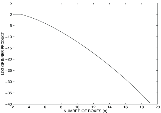
Figure 1: A plot showing $\log\left|{{\cal O}\over{\cal N}_{S}{\cal N}_{A}}\right|$ as a function of the number of boxes $n$, for $N=20$.

In the case when $n$ is of order $\sim N$, our operators are dual to heavy objects whose wave functions will be well localized in the bulk of the AdS space. For these states we expect much less mixing of the boundary and bulk degrees of freedom. Consequently, we don’t expect that the boundary degrees of freedom make a large contribution to the state, and the difference between the operators in the $SU(N)$ gauge theory and the $U(N)$ gauge theory is not great. In this case we do expect to inherit the orthogonality of the $U(N)$ operators.

4.2 Finite $N$

At finite $N$, there is not even an approximate notion of single eigenvalue dynamics. In this case, perhaps the simplest way forward is to apply the Gram-Schmidt algorithm to the linearly independent operators selected in section 3.4 to obtain a new set of operators which do diagonalize the inner product. This process can be used to produce many different sets of operators diagonalizing the two point function. Which set is the most useful for the gauge theory/gravity dictionary? We do not have a satisfactory answer to this question.

Although the Gram-Schmidt algorithm can be used to diagonalize the two point function, this does not give a practical solution when the number of boxes in the Young diagrams becomes large. Is there a more elegant way to perform the orthogonalization?

The orthogonality of Schur polynomials in the $\Phi$ field was proved using the Frobenius-Schur duality between the symmetric and unitary groups[2]. It is natural to ask if there is a generalization of these results for the Schur polynomials in the $\Psi$ field. There is a simple possibility that can be considered. Irreducible representations of the unitary groups are obtained by taking contractions of objects transforming in the fundamental representation with tensors that have a definite symmetry under interchange of indices. Irreducible representations of the orthogonal groups are obtained by taking contractions with traceless tensors that have a specific symmetry under interchange of indices. One might guess that this tracelessness constraint is exactly what is needed to solve the problem studied here.

The relevance of the permutation group for Frobenius-Schur duality comes from the fact that the permutation group and unitary groups are centralizers of each other. The centralizers of the orthogonal group are the Brauer algebras. Thus, one may have suspected that the polynomials (in $\Psi$) built by replacing the characters of the permutation group in the Schur polynomials by the characters of the Brauer algebra would have diagonal two point functions. We have explicitly checked that this guess is not correct.

4.3 Giant Gravitons as probes of the Dual Geometry

Natural probes of the dual geometry are heavy objects which can be treated semiclassically. The mass of the object is set by the scale on which the geometry is to be probed. If a scale $\gamma$ is to be resolved, the fluctuations in the position of the probe must be less than $\gamma$, forcing the mass of the probe to be larger than $\gamma^{-1}$. Of course, there is a smallest scale which can be probed. At this smallest scale the probe starts to noticeably deform the background metric, that is, its gravitational radius is no longer smaller than $\gamma$. This smallest scale is the Planck scale.

When the gauge theory is at strong coupling, the radius of AdS is much larger than the string scale. In this limit and at geometric distances which are larger than the string scale, we’d expect that giant gravitons are good probes of the geometry.

For the gravity dual to the $U(N)$ gauge theory, since there are both bulk and boundary degrees of freedom, it is not good enough to simply require a heavy probe. Indeed, we could imagine a composite object composed of a heavy excitation of boundary modes and a light excitation of the bulk gravity. Even if the mass of the composite is larger that $\gamma^{-1}$, this probe might not resolve features in the bulk of order $\gamma$. In this context, it is appropriate to ask if we can separate the bulk and boundary contributions to operators in the dual gauge theory.

4.4 Disentangling bulk and boundary degrees of freedom

Up to this point, we have used a ghost field $c$ to subtract the mode corresponding to the trace of $\Phi$. It is also possible to express $\Phi$ in terms of $\Psi$ by adding the mode corresponding to the trace. In terms of the $b$ field

$$\langle bb\rangle=\langle b^{*}b^{*}\rangle,\qquad\langle bb^{*}\rangle={1\over N},$$

we have the identity

$$\langle F(\Phi_{ij},\Phi_{kl}^{*})\rangle=\langle F(\Psi_{ij}+b\delta_{ij},\Phi_{kl}^{*}+b^{*}\delta_{kl})\rangle,$$

for an arbitrary function $F(\cdot,\cdot)$. In contrast to our previous computations, where the ghost had no physical meaning, $b$ and $\Psi$ do have clear physical interpretations. $b$ describes the overall center of mass motion of all of the branes; in the gravity dual it is localized on the boundary of $AdS_{5}\times S^{5}$. $\Psi$ is describing the bulk string theory. The technology we have developed above can now be used to disentangle bulk and boundary degrees of freedom in the dual super Yang-Mills theory. For concreteness, consider the operator dual to a sphere giant, that is, a Schur polynomial corresponding to an antisymmetric representation with $n$ boxes and $n\sim N$. This operator is dual to a heavy state and so should provide a good (well localized) probe of the geometry of the gravitational theory.

Let ${\cal R}_{n}$ denote the Young diagram with a single column and $n$ rows. If $n=0$, ${\cal R}_{n}=1$. Then, we have

$$\chi_{{\cal R}_{n}}(\Phi)\to\chi_{{\cal R}_{n}}(\Psi+b{\bf 1})=\sum_{i=0}^{n}{b^{i}\over i!}\prod_{k=1}^{i}(N-n+k)\chi_{{\cal R}_{n-i}}(\Psi).$$

Terms in the above sum corresponding to low values of $i$ are the product of a Schur polynomial corresponding to a representation with a large number of boxes and a boundary state with a small ${\cal R}$ charge. Thus, these terms correspond to objects in the bulk gravity which are heavy and hence well localized times light boundary excitations which will not be well localized. Terms corresponding to large values of $i$ are the product of a Schur polynomial corresponding to a representation with a small number of boxes and a boundary state with a large ${\cal R}$ charge. Thus, these terms correspond to objects in the bulk gravity which are light and hence not well localized times heavy boundary excitations which will be well localized. To understand why, in spite of this, the Schur polynomials still provide localized probes, recall that the two point functions of the Schur polynomials are not normalized. To estimate how large the different contributions to $\chi_{R}(\Phi)$ are, we should work with properly normalized operators. In terms of ${b^{\prime n}\over\sqrt{n!}}$ and $\bar{\chi}_{{\cal R}_{n}}(\Psi)$, with

$$\langle{{b}^{\prime i}\over\sqrt{i!}}\bar{\chi}_{{\cal R}_{n-i}}(\Psi){b^{\prime*j}\over\sqrt{j!}}\bar{\chi}_{{\cal R}_{n-j}}(\Psi^{*})\rangle=\delta_{ij},$$

we have

$$\chi_{{\cal R}_{n}}(\Phi)\to\chi_{{\cal R}_{n}}(\Psi+b{\bf 1})=\sum_{i=0}^{n}\alpha_{i}{b^{\prime i}\over\sqrt{i!}}\bar{\chi}_{{\cal R}_{n-i}}(\Psi),$$

with

$$\alpha_{i}={(N-n+i)!\over(N-n)!}{{\cal N}_{A}(n-i)\over\sqrt{N^{i}i!}},\qquad{\cal N}_{A}^{2}(n)={N!\over(N-n)!}\sum_{i=0}^{n}{(-1)^{i}\over N^{i}}{(N+i-n)!\over i!(N-n)!}.$$

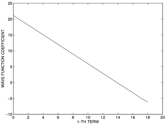
Figure 2: This plot shows the components in the operator dual to a sphere giant. $\log\left|\alpha_{i}\right|$ is plotted as a function of $i$, for $N=20$ and $n=20$.

Clearly, the above expansion for the operator $\chi_{{\cal R}_{n}}(\Phi)$ is dominated by terms corresponding to low values of $i$. Consequently, the contribution from the boundary degrees of freedom to these operators is exponentially suppressed. Thus, the $\chi_{{\cal R}_{n}}(\Phi)$ do provide localized probes of the dual geometry.

What we have found is that, in the large $N$ limit and for $n\sim N$ boxes, the dependence on the $b$ modes is suppressed. Consequently Schur polynomials for the totally antisymmetric representations in $\Phi$ essentially coincide with Schur polynomials for the totally antisymmetric representations in $\Psi$. Evidently Schur polynomials in the $SU(N)$ theory corresponding to the totally antisymmetric representations with $n\sim N$ boxes again provide the duals to sphere giants.

Finally, the corresponding discussion for AdS giants is equally straightforward. In this case we have (in what follows ${\cal S}_{n}$ denotes a Young diagram with a single row of $n$ boxes)

$$\chi_{{\cal S}_{n}}(\Phi)\to\chi_{{\cal S}_{n}}(\Psi+b{\bf 1})=\sum_{i=0}^{n}\alpha_{i}{b^{\prime i}\over\sqrt{i!}}\bar{\chi}_{{\cal S}_{n-i}}(\Psi),$$

with

$$\alpha_{i}={(N+n-1)!\over(N+n-i-1)!}{{\cal N}_{S}(n-i)\over\sqrt{N^{i}i!}},\qquad{\cal N}_{S}^{2}(n)={(N+n-1)!\over(N-1)!}\sum_{i=0}^{n}{(-1)^{i}\over N^{i}}{(N+n-1)!\over i!(N+n-i-1)!}.$$

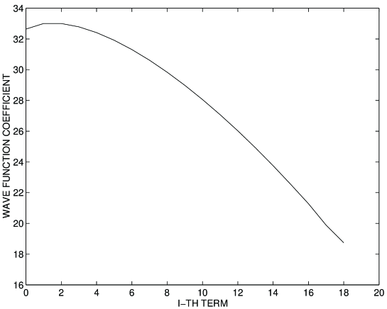
Figure 3: This plot shows the components in the operator dual to an AdS giant. $\log\left|\alpha_{i}\right|$ is plotted as a function of $i$, for $N=20$ and $n=20$.

It is interesting to note that the coefficients $\alpha_{i}$ reach a maximum at $i=1,2$. For these terms there is a very small contribution coming from the boundary degrees of freedom. Clearly however, the boundary contribution is still significantly suppressed.

5 Summary

The results of [2] provide a set of operators, the Schur polynomials, which have diagonal two point functions and are in one-to-one correspondence with the half-BPS representations of the $U(N)$ gauge theory at zero coupling and finite $N$. Obtaining the corresponding result for the $SU(N)$ gauge theory was one of the goals of this article.

We have developed the necessary technology to study Schur polynomials in the $SU(N)$ gauge theory. In addition, we have obtained a complete set of relations between the Schur polynomials and have provided an algorithm which selects a unique linearly independent basis for the half-BPS representations. Using the Gram-Schmidt algorithm we can obtain a new set of operators with diagonal two point functions. Although this answer is not very explicit, it does provide the generalization we were after.

We have argued that at large $N$ Schur polynomials corresponding to either totally symmetric or totally antiymmetric representations with a large number of boxes, are approximately dual to giant graviton states. Using the techniques developed in section 3, we were able to study the two point function of these two operators and verify that it goes to zero exponentially fast as the number of boxes is increased.

Further, our technology when applied to the $U(N)$ gauge theory allows for a separation of the bulk and boundary degrees of freedom. We have verified that for both sphere giants and AdS giants, the boundary contribution is small enough for the Schur polynomials of the $SU(N)$ gauge theory to remain good candidate duals to giant gravitons.

Acknowledgements: We would like to thank Eric Gimon, Antal Jevicki, João Rodrigues and especially Sanjaye Ramgoolam for pleasant discussions and David Berenstein for helpful correspondence. We would also like to thank Sanjaye for helpful comments on the manuscript. This work is supported by NRF grant number Gun 2047219.

References

-
[1]
J. Maldacena, The large N limit of superconformal field theories and supergravity,
hep-th/9711200, Adv. Theor. Math. Phys. 2 231 (1998);
S. Gubser, I.R. Klebanov and A.M. Polyakov, Gauge Theory Correlators from Non-critical String Theory, hep-th/9802109, Phys. Lett. B428 (1998) 105;
E. Witten, Anti-de Sitter Space and Holography, hep-th/9802150, Adv. Theor. Math. Phys. 2 (1998) 253. -
[2]
S. Corley, A. Jevicki and S. Ramgoolam, Exact Correlators of
Giant Gravitons from Dual SYM Theory, hep-th/0111222, Adv. Theor. Math.
Phys. 5, 809-839, 2002;
- [3] S. Corley and S. Ramgoolam, Finite Factorization equations and sum rules for BPS Correlators in N=4 SYM Theory, hep-th/0205221, Nucl. Phys. B641, 131-187, 2002.
- [4] G.W. Gibbons and P.K. Townsend, Vacuum Interpolation in Supergravity via Super p-Branes, hep-th/9307049, Phys. Rev. Lett. 71 (1993) 3754.
-
[5]
C. Frondsal, The Dirac Supermultiplet, Phys. Rev. D26 (1982) 1988;
K. Pilch, P. van Nieuwenhuizen and P.K. Townsend, Compactification of D=11 Supergravity on (Or 11= 7+4 too), Nucl. Phys. B242 (1984) 377;
Eric Bergshoeff, Abdus Salam, Ergin Sezgin and Yoshiaki Tanii, Singletons, Higher Spin Massless States and the supermembrane, Phys.Lett.B205 (1988) 237;
Eric Bergshoeff, Abdus Salam, Ergin Sezgin and Yoshiaki Tanii, N=8 Supersingleton Quantum Field Theory, Nucl.Phys.B305 (1988) 497;
E. Bergshoeff, M.J. Duff, C.N. Pope and E. Sezgin, Compactifications of the Eleven dimensional Super membrane, Phys.Lett.B224 (1989) 71. - [6] Ofer Aharony, Steven S. Gubser, Juan M. Maldacena, Hirosi Ooguri and Yaron Oz, Large N Field Theories, String Theory and Gravity, hep-th/9905111 Phys.Rept.323 (2000) 183.
- [7] D. Berenstein, A Toy Model for the AdS/CFT Correspondence, hep-th/0403110
- [8] R. Myers, Dielectric-Branes, hep-th/9910053, JHEP 9912 022 (1999).
- [9] J. McGreevy, L. Susskind and N. Toumbas, Invasion of the Giant Gravitons from Anti-de Sitter Space, hep-th/0003075, JHEP 0006 008 (2000).
-
[10]
S. Das, A. Jevicki and S. Mathur, Vibration Modes of Giant Gravitons,
hep-th/0009019, Phys. Rev. D63 024013 2001;
S. Das, A. Jevicki and S. Mathur, Giant Gravitons, BPS Bounds and Noncommutativity, hep-th/0008088, Phys. Rev. D63 044001 2001;
M.T. Grisaru, R.C. Myers and O. Tajford, SUSY and Goliath, hep-th/0008015, JHEP 0008 040 (2000);
A. Hashimoto, S. Hirano and N. Itzakhi, Large Branes in AdS and their Field Theory Dual, hep-th/0008016, JHEP 0008 051 (2000). -
[11]
J. Maldacena and A. Strominger, AdS3 Black Holes and a Stringy Exclusion
Principle, JHEP 9812 005 (1998);
S. Gubser, Can the effective string see higher partial waves? hep-th/9704195, Phys. Rev. D56 (1998) 4984. -
[12]
A.Jevicki and S.Ramgoolam, Non-commutative gravity from the AdS/CFT correspondence,
hep-th/9902059, JHEP 9904 (1999) 032;
P.M. Ho, S.Ramgoolam and R. Tatar, Quantum Spacetimes and Finite Effects in 4-D SYM Theories, hep-th/9907145, Nucl.Phys. B573 (2000) 364;
P.M. Ho and M. Li, Fuzzy Spheres in AdS/CFT Correspondence and Holography from Noncommutativity, hep-th/0004072, Nucl.Phys. B596 (2001) 259. - [13] J. Lee, Tunneling between the Giant Gravitons in , hep-th/0010191, Phys. Rev. D64 (2001) 046012.
-
[14]
O. Aharony, Y.E. Antebi, M. Berkooz and R. Fishman, Holey sheets: Pfaffians and
subdeterminants as D-brane operators in large gauge theories, hep-th/0211152,
JHEP 0212 (2002) 069;
D. Berenstein, Shape and Holography: Studies of dual operators to giant gravitons, hep-th/0306090, Nucl. Phys. B675 (2003) 179;
V. Balasubramanian, M.X. Huang, T.S. Levi and A. Naqvi, Open Strings from super Yang-Mills, hep-th/0204196, JHEP 0208 (2002) 037. - [15] D. Berenstein, J. Maldacena and H. Nastase, Strings in Flat Space and pp-Waves from N=4 Super Yang-Mills, hep-th/0202021, JHEP 0204 (2002) 013.
- [16] E. Brezin, C. Itzykson, G. Parisi and J.B. Zuber, Planar Diagrams, Commun. Math. Phys. 59 (1978) 35.
- [17] V. Balasubramanian, M. Berkooz, A. Naqvi and M. Strassler, Giant Gravitons in Conformal Field Theory, hep-th/0107119, JHEP 0204 (2002) 034.
- [18] H. Lin, O. Lunin and J. Maldacena, Bubbling AdS space and 1/2 BPS geometries, hep-th/0409174.
-
[19]
A. Jevicki and A. van Tonder, Finite q-oscillator Description of 2D String Theory,
hep-th/9601058, Mod. Phys. Lett. A11 (1996) 1397;
A.P. Polychronakos, Quasihole wavefunctions for the Calogero Model, cond-mat/9603132, Mod. Phys. Lett. A11, (1996) 1273. - [20] A. Jevicki, Non-perturbative Collective Field Theory, Nucl. Phys. B376 (1992) 75.
-
[21]
The relation between free fermions and Young diagrams is an old one. See for example:
M.R. Douglas, Conformal Field Theory Techniques for Large N Group Theory, hep-th/9303159;
M.R. Douglas, Conformal Field Theory Techniques in Large N Yang-Mills Theory, hep-th/9311130;
J. Minahan and A. Polychronakos, Equivalence of Two Dimensional QCD and the c=1 Matrix Model, hep-th/9303153Nucl. Phys. B422 (1993) 155.
For a review, see
S. Cordes, G. Moore and S. Ramgoolam, Lectures on 2D Yang-Mills Theory, Equivariant Cohomology and Topological Field Theories, hep-th/9411210. -
[22]
J. McGreevy and H. Verlinde, String from Tachyons: The c=1 Matrix Model Reloaded,
hep-th/0304224, JHEP 0312 (2003) 054;
J. McGreevy, J. Teschner and H. Verlinde, Classical and quantum D-branes in 2D string theory, hep-th/0305194, JHEP 0401 (2004) 039;
M.R. Douglas, I.R. Klebanov, D. Kutasov, J. Maldacena, E. Martinec and N. Seiberg, A new hat for the c=1 matrix model, hep-th/0307195;
D. Gaiotto, N. Itzhaki and L. Rastelli, On the BCFT description of holes in the c=1 matrix model, hep-th/0307221, Phys. Lett. B575 (2003) 111. - [23] See for example, H. Georgi, Lie Algebras in Particle Physics, First Edition, chapter XIII SU(N).
- [24] M.M. Sheikh-Jabbari, Tiny Graviton Theory: DLCQ of IIB Plane-Wave String Theory, A Conjecture, hep-th/0406214, JHEP 0409 (2004) 017.
-
[25]
M.M. Caldarelli and P.J. Silva, Giant Gravitons in AdS/CFT (I):Matrix Model and
Back Reaction, hep-th/0406096, JHEP 0408 (2004) 029
M.M. Caldarelli and P.J. Silva, Multi Graviton Systems, SUSY Breaking and CFT, hep-th/0401213, JHEP 0402 (2004) 052. -
[26]
S. Prokushkin and M.M. Sheikh-Jabbari, Squashed Giants: Bound States of Giant
Gravitons, hep-th/0406053, JHEP 0407 (2004) 077;
D. Sadri and M.M. Sheikh-Jabbari, Giant Hedgehogs: Spikes on Giant Gravitons, hep-th/0312155, Nucl. Phys. B687 (2004) 161. - [27] A. Ram, Characters of Brauer’s Centralizer Algebras, Pac. Jour. Math. 169, (1995) 173.