Abstract

We consider tunneling transitions between states separated by an energy barrier in a simple field theoretical model. We analyse the case of soliton creation induced by collisions of a few highly energetic particles. We present semiclassical, but otherwise first principle, study of this process at all energies of colliding particles. We find that direct tunneling to the final state occurs at energies below the critical value $E_{c}$, which is slightly higher than the barrier height. Tunneling probability grows with energy in this regime. Above the critical energy, the tunneling mechanism is different. The transition proceeds through creation of a state close to the top of the potential barrier (sphaleron) and its subsequent decay. At certain limiting energy $E_{l}$ tunneling probability ceases to grow. At higher energies the dominant mechanism of transition becomes the release of energy excess $E-E_{l}$ by the emission of a few particles and then tunneling at effectively lower energy $E=E_{l}$ via the limiting semiclassical configuration. The latter belongs to a class of “real–time instantons”, semiclassical solutions saturating the inclusive probability of tunneling from initial states with given number of particles. We conclude that the process of collision–induced tunneling is exponentially suppressed at all energies.

1 Introduction

Tunneling processes are inherent in many field theoretical models, well–known examples being false vacuum decay in scalar theories [1] and topology–changing transitions in gauge theories [2]. To some extent tunneling in field theory is similar to that in quantum mechanics. A relevant energy scale for tunneling is set by the minimum height of the energy barrier separating initial and final states. It is equal to the energy of a critical bubble [1] and sphaleron [3] in the two examples above. Classical transition is energetically forbidden at energies below the barrier height. In the weak coupling regime semiclassical technique is applicable for the description of tunneling, and the rate of transition is exponentially suppressed. On the other hand, one might expect the suppression to vanish once large enough amount of energy, lifting the system above the potential barrier, is injected. This expectation turns out to be correct in some situations, such as transitions at finite temperature (see Ref. [4] and references therein), at non-zero fermion density [5], or in the presence of heavy particles in the initial state [6, 7]. There is, however, a situation which seems to provide a notable exception from this rule. This is the case of tunneling induced by collision of two highly energetic particles.

A prospect of observation of non–perturbative transitions in particle collisions [8, 9] provoked extensive discussion in literature (see [10, 11, 4] for reviews). Semiclassical results [12, 13, 14] show, however, that this process of induced tunneling remains exponentially suppressed even when the energy of colliding particles exceeds considerably the height of the potential barrier. Furthermore, investigations of toy models [15, 16] and unitarity arguments [17, 18, 19] indicate that the process of induced tunneling should remain exponentially suppressed even as the energy of collision tends to infinity. Nevertheless, no direct calculation of the suppression exponent at very large energies of colliding particles has been carried out so far in any model, not to speak about the limit of infinite energy.

In this paper we consider a simple field theoretical model allowing for the semiclassical calculation of the suppression exponent of induced tunneling at all energies of colliding particles. The model describes free scalar field $\phi(t,{\rm x})$ living in (1+1) dimensions on a half–line ${\rm x}>0$, with interactions localized at the boundary point ${\rm x}=0$. The action of the model is

$$S=\frac{1}{2}\int dt\int\limits_{0}^{\infty}d{\rm x}\left[(\partial_{\mu}\phi)^{2}-m^{2}\phi^{2}\right]-\frac{\mu}{g^{2}}\int dt\left[1-\cos(g\phi(t,0))\right].$$ (1)

The second term represents boundary interaction with the characteristic energy scale $\mu$. The bulk mass $m$ is introduced as an infrared regulator, and it is assumed to be small compared to the scale $\mu$. In the main body of the paper we take the limit $m\to 0$, as the small mass turns out to be irrelevant for the semiclassical evaluation of the suppression exponent. The only role it plays is to fix the free particle basis for the asymptotic states.

The massless version of the model (1) with different infrared regularizations has been considered in several contexts. In condensed matter physics it has been used to describe transport in quantum wires [20] and Josephson chains with defects [21], the role of the regulator in those cases being played by the length of wire or chain. In [22], a special value of the coupling constant $g=\sqrt{2\pi}$ was considered and the model was shown to be exactly solvable in that case. Finally, in [23] the model (1) with $m=0$, obtained as a limit of a model with sine-Gordon interaction in the bulk, was argued to be integrable at any value of $g$.

The model (1) possesses a number of static solutions determined by the value of the field at ${\rm x}=0$. Up to corrections of order $m/\mu$, these solutions have the following form: the value of the field at the boundary is “pinned down” to one of the minima of the boundary potential, $\phi_{0}^{(n)}=2\pi n/g$, $n=1,2,\dots$, while in the bulk the field slowly falls off due to the presence of the small mass,

$$\phi_{\mathrm{sol}}^{(n)}({\rm x})=\phi_{0}^{(n)}\mathrm{e}^{-m\mathrm{x}}\;.$$

These solutions are localized near the boundary, ${\rm x}=0$, so it is natural to call them “boundary solitons”. The masses of the solitons,

$$M^{(n)}=\frac{2\pi^{2}n^{2}}{g^{2}}m\;,$$ (2)

are relatively small, as they are proportional to the bulk mass $m$.

In this paper we study the process of creation of the first soliton ($\phi_{0}^{(1)}=2\pi/g$) in a collision of a particle (or a bunch of particles) with the boundary; the energy of the particle(s) is assumed to be much larger than the soliton mass. To start with, let us consider the classical analog of this process, which is the creation of the soliton in the collision of a classical wave packet with the boundary. It is easy to see that the classical process is possible only if the energy of the wave packet exceeds some threshold energy $E_{S}$, which is much higher than the soliton mass (2). Indeed, the boundary value $\phi(t,0)$ of the relevant classical solution changes from $0$ to $2\pi/g$ during the process. The classical solution passes the maximum of the boundary potential $\phi_{0}^{(S)}=\pi/g$ at some moment of time, and thus the total energy of this solution is larger than the boundary energy at the maximum,

$$E_{S}=\frac{2\mu}{g^{2}}\;.$$ (3)

One concludes that any state containing boundary soliton is separated from the vacuum by a potential barrier. It is straightforward to find static configuration “sitting” on top of the barrier, which we call “sphaleron” following Ref. [3]. This is an unstable static solution of the classical field equations representing the saddle point of the static energy functional. In our model it has the same exponential form as the soliton but with the boundary value on top of the boundary potential,

$$\phi_{S}=\frac{\pi}{g}\mathrm{e}^{-m\mathrm{x}}\;.$$

The energy of the sphaleron is given by Eq. (3), again up to corrections of order $m/\mu$.

We see that the soliton production in collisions of particle(s) with the boundary is classically forbidden and hence exponentially suppressed at energies smaller than the sphaleron energy. The question is what happens when energy grows. In this paper we study this question by applying semiclassical methods. The semiclassical approximation is justified by the following observation. After the rescaling of the field, $\phi\to\phi/g$, the coupling constant $g$ enters the action only through the overall multiplicative factor $1/g^{2}$. Therefore, $g^{2}$ plays the role of the Planck constant $\hbar$, and the weak coupling limit corresponds to the semiclassical situation. This is the case we consider in this paper.

The techniques we use are explained in more detail in subsequent sections. Here we briefly summarize our results. We calculate semiclassically the probability ${\cal P}$ of the soliton production in collision of a particle with the boundary. In the leading semiclassical approximation it has the exponential form,

$${\cal P}\propto\mathrm{e}^{-F/g^{2}},$$

and we concentrate on the calculation of the suppression exponent $F$.

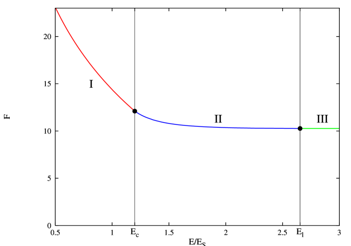
Figure 1: Dependence of the suppression exponent $F$ on the collision energy $E$, the latter measured in units of the sphaleron energy $E_{S}=2\mu/g^{2}$. The tunneling process is driven by three physically different mechanisms in the parts I, II, III of the graph.

Our results for the dependence of the suppression exponent on the energy of incoming particle are shown in Fig. 1. There are three energy regions corresponding to three physically different mechanisms of the process. If the collision energy is lower than the critical value $E_{c}\approx 1.2E_{S}$ (region I of the figure), tunneling occurs in conventional way with the relevant semiclassical configurations ending up directly in the soliton sector. This regime can be called “direct tunneling”. We study this region of energies in Sec. 3, and find the analytic result for the suppression of such transitions:

$$F(E)=4\pi\mathop{\rm ln}\nolimits\left[\frac{\pi E_{S}}{E}\right],\;\;\;E<E_{c}\;.$$ (4)

Formula (4), if continued to the energies higher than the critical energy $E_{c}$, would show that the transitions become unsuppressed at energy $\pi E_{S}$. However, this formula is incorrect at $E>E_{c}$, as the solutions describing direct tunneling cease to exist at energies higher than the critical one.

Semiclassical configurations with energies above $E_{c}$ are studied in Sec. 4 using a combination of analytic and numerical methods. We find that their properties are different from the ones below the critical energy, and the tunneling mechanism they describe is entirely different. Instead of tunneling directly to the other side of the energy barrier, the system jumps on its top, thus creating the sphaleron which then decays producing the soliton in the final state. The second stage of the process, decay of the sphaleron into the soliton, proceeds with the probability of order one. Still, the transitions remain exponentially suppressed due to considerable rearrangement the system has to undergo during the first stage of the process, i.e. formation of the sphaleron. The tunneling mechanism outlined here has been observed recently in quantum mechanics [28] and gauge theory [14]. Transitions of this type correspond to the region II of Fig. 1, they extend up to the energy $E_{l}\approx 2.7\;E_{S}$.

The solution describing the transition with the energy $E_{l}$ belongs to a novel class of semiclassical solutions which we call “real–time instantons”. The latter saturate the inclusive probability of tunneling from initial states with given number of particles. We consider the real–time instantons in Sec. 4.3.

The energy $E_{l}$ is the best energy for the transition. Further increase of energy above $E_{l}$ (region III of Fig. 1) does not lead to any gain in the transition probability, and the suppression exponent stays constant all the way up to $E=\infty$. We show in Sec. 4.4 that the system emits the energy excess $(E-E_{l})$ in the form of a few highly energetic particles, and then undergoes the transition of the second type (on top of the energy barrier) with the energy $E_{l}$. Emission of one or several particles does not change the suppression exponent, affecting only the pre-exponential factor. In this way we obtain that $F(E>E_{l})=10.27$. Our results confirm the conjecture [24] that the suppression exponent of collision–induced tunneling is frozen at high energies. The tunneling mechanism at $E>E_{l}$, i.e. emission of energy excess in the form of a few particles and tunneling via the most favourable semiclassical configuration, coincides with that conjectured in Ref. [15].

Section 5 contains concluding remarks.

2 $T/\theta$–problem

2.1 General formalism

A difficulty one encounters in the semiclassical description of collision–induced tunneling is that the initial state of the process is not semiclassical. To this end, the method of calculation should be appropriately adjusted. In this work we adopt the method proposed in [25]. Namely, let us consider the inclusive probability of tunneling from multiparticle states with energy $E$ and number of particles $N$:

$${\cal P}(E,N)=\sum\limits_{i,f}\left|\langle f|\hat{\cal S}\hat{P}_{E}\hat{P}_{N}|i\rangle\right|^{2}\;,$$ (5)

where $\hat{\cal S}$ is the $S$-matrix while $\hat{P}_{E}$ and $\hat{P}_{N}$ are projectors onto states with given energy and number of particles. The states $|i\rangle$ and $|f\rangle$ are perturbative excitations above the vacuum and the soliton, respectively. The function (5) can be calculated with the use of semiclassical methods, provided that the energy and initial number of particles are semiclassically large, $E=\tilde{E}/g^{2}$, $N=\tilde{N}/g^{2}$. The result has the exponential form,

$${\cal P}(E,N)\propto\mathrm{e}^{-F(\tilde{E},\tilde{N})/g^{2}}\;.$$

It is clear that the multiparticle probability ${\cal P}(E,N)$ provides an upper bound on the tunneling probability induced by collisions of fewer particles. Indeed, any initial few–particle state can be promoted to a multiparticle one by adding an appropriate number of “spectator” particles which do not affect the tunneling process. Thus, the exponent $F(\tilde{E})$ of the soliton production in the collision of one particle with the boundary, is larger than the inclusive suppression exponent $F(\tilde{E},\tilde{N})$. Furthermore, one conjectures [25] that the small–particle limit of the multiparticle exponent coincides with the exponent of tunneling induced by one or a few particles,

$$F(\tilde{E})=\lim_{\tilde{N}\to 0}F(\tilde{E},\tilde{N})\;.$$ (6)

The relation (6) has been checked in several orders of perturbation theory around the instanton in gauge theory [26], and also non-perturbatively in quantum mechanics of two degrees of freedom [27, 28]. We use Eq. (6) throughout this paper to obtain $F(\tilde{E})$ from the multiparticle exponent $F(\tilde{E},\tilde{N})$. To simplify notations, we omit tilde over the rescaled energy and number of particles below.

Transitions with fixed initial number of particles $N$ are described by solutions of the so–called $T/\theta$ boundary value problem [25]. The latter is formulated on the contour $ABCD$ in complex time plane shown in Fig. 2.

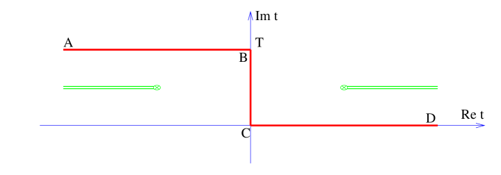
Figure 2: Contour in complex time on which the boundary value problem is formulated.

Namely, the configurations describing tunneling should satisfy the classical field equations in the internal points of the contour,

$$(\partial^{2}_{t}-\partial^{2}_{\rm x}+m^{2})\phi=0,\;\;{\rm x}>0\;,$$ (7a)

$$\partial_{\rm x}\phi=\mu\sin\phi,\;\;{{\rm x}=0}\;.$$ (7b)

The Euclidean part $$BC T A D \phi(t,{\rm x}) t\to+\infty$$ of the contour may be interpreted as representing the evolution of the field under the barrier, “duration” of this evolution is a parameter of solution. Field equations (7a), (7b) are supplemented by initial and final boundary conditions in the parts and of the contour, respectively. Namely, the field should be real as ; it describes the final state of the semiclassical evolution,

$$\mathrm{Im}\;\phi\to 0\;\;\mathrm{as}\;\;t\to+\infty\;.$$ (7c)

The field in the initial state is linear about the vacuum $$\phi=0$$,

$$\phi(t^{\prime}+iT,{\rm x})\Bigg{|}_{t^{\prime}\to-\infty}=\frac{1}{(2\pi)^{1/2}}\int\frac{dk}{\sqrt{2\omega_{k}}}\left(f_{k}\mathrm{e}^{-i\omega_{k}t^{\prime}+ik{\rm x}}+g_{k}^{*}\mathrm{e}^{i\omega_{k}t^{\prime}-ik{\rm x}}\right)\;,$$ (7d)

and the boundary conditions in the part $$A$$ of the contour relate positive and negative frequency components of the solution,

$$f_{k}=\mathrm{e}^{-\theta}g_{k}\;.$$ (7e)

The boundary condition (7e) can be understood as follows. In the limit $\theta\to+\infty$ it coincides with the Feynman boundary condition and thus corresponds to the initial state with semiclassically small number of particles. Finite $\theta$ corresponds to the initial state with non–zero $N$, from which tunneling occurs in the least suppressed way.

Given the values of $T$ and $\theta$, one finds a complex solution $\phi(t,{\rm x};T,\theta)$ satisfying equations (7a) — (7e). The energy and initial number of particles for this solution are given by the familiar formulae,

$$E=\int dk\;\omega_{k}f_{k}g_{k}^{*}\;,$$ (8a)

$$N=\int dk\;f_{k}g_{k}^{*}\;.$$ (8b)

Alternatively, they can be determined by differentiating the action functional evaluated on the solution, with respect to the parameters $T$ and $\theta$,

$$E=\frac{\partial}{\partial T}\;\mathrm{Im}S(T,\theta)\;,\;\;\;N=2\frac{\partial}{\partial\theta}\;\mathrm{Im}S(T,\theta)\;,$$ (9)

where

$$S=\frac{1}{2}\int dt\int_{0}^{\infty}d{\rm x}~{}[-\phi\partial_{0}^{2}\phi-(\partial_{\rm x}\phi)^{2}-m^{2}\phi^{2}]-\mu\int dt~{}(1-\cos{\phi(t,0)})$$ (10)

is the action of the model, integrated by parts and calculated along the contour $ABCD$. The suppression exponent of the process is given by the Legendre transform of the action functional,

$$F(E,N)=2\mathop{\rm Im}\nolimits{S}-N\theta-2ET\;.$$ (11)

Below we refer to the problem (7) as “$T/\theta$-problem”, and use the term “$\theta$–instanton” for the relevant semiclassical solution.

Several remarks are in order. First, the boundary value problem (7) does not guarantee that its solutions interpolate between states with and without the soliton. In the next subsection we describe additional requirements that should be imposed to ensure that the solutions are relevant for tunneling.

Second, one observes that the solution $\phi(t,{\rm x})$ can be analytically continued to the complex time plane, and in this way the contour $ABCD$ may be deformed without affecting the integral (11) for the suppression exponent. The only thing one should worry about while deforming the contour is to avoid the singularities of the solution, which are shown schematically by the double lines in Fig. 2. Below it will be convenient not to be attached to a contour of any particular form. Instead, we look for the solution $\phi(t,{\rm x})$ satisfying Eqs. (7a), (7b) in the entire complex time plane, with boundary conditions (7c) and (7e) imposed in the asymptotic regions $D$ and $A$ of the complex plane. When using this approach, one should make sure, however, that the asymptotic regions $A$ and $D$ can be connected by a contour avoiding the singularities of solution.

Finally, let us discuss two particular limits of the boundary value problem (7). The first one corresponds to $\theta=0$. Solutions obtained in this limit are periodic in Euclidean time, they are called “periodic instantons” [29]. These solutions determine the inclusive probability of tunneling from states with given energy and arbitrary number of particles,

$${\cal P}_{p}(E)=\sum\limits_{i,f}\left|\langle f|\hat{\cal S}\hat{P}_{E}|i\rangle\right|^{2}\;.$$

Periodic instantons have been extensively studied in literature [30], in particular, they can be used to determine the rate of transitions at finite temperature.

Below we will encounter solutions of the $T/\theta$-problem obtained in the limit $T=0$. To the best of our knowledge, such solutions have never been considered before. We call them “real-time instantons”, as the contour $ABCD$ does not contain a Euclidean part in this case. These solutions depend on a single auxiliary parameter $\theta$, i.e. a single free physical parameter of the incoming state, which we choose to be the number of particles $N$. The energy is thus a function of $N$ for this set of solutions. The value of the suppression exponent $F_{rt}(N)$ evaluated on the real-time instantons is non-zero exclusively due to the fact that these field configurations are complex-valued. At first sight, the latter property may seem to contradict the condition (7c) requiring reality of the solution in the region $D$ of the real axis. However, this is not the case: the condition (7c) is imposed only in the asymptotic future, and it does not prevent the solution from being complex–valued at finite times. Let us discuss this point in more detail. Assume that at large (but finite) time the solution is linearized about some static configuration,

$$\phi(t,{\rm x})=\phi_{0}({\rm x})+\delta\phi_{1}(t,{\rm x})+i\delta\phi_{2}(t,{\rm x})\;,$$

where both $\delta\phi_{1}$ and $\delta\phi_{2}$ are real. The condition (7c) implies that $\delta\phi_{2}\to 0$ at $t\to+\infty$. This amounts to requiring that $\delta\phi_{2}$ describes the evolution along the negative mode of the static solution $\phi_{0}({\rm x})$, so that $\delta\phi_{2}\propto{\rm e}^{-{\rm const}\cdot t}$. Thus, the configuration $\phi_{0}({\rm x})$ must have negative modes, in other words, it must be unstable. The only candidate for $\phi_{0}({\rm x})$ in our case is the sphaleron. We arrive at the important conclusion that the real–time instantons describe formation of the sphaleron at $t\to+\infty$. It is worth noting that this observation refers, in fact, to any $\theta$-instanton which is not real at real time, cf. Ref. [28].

Let us demonstrate that the real-time instantons determine the suppression exponent for the inclusive probability of tunneling from states with given number of incoming particles and arbitrary energy

$${\cal P}(N)=\sum\limits_{i,f}\left|\langle f|\hat{\cal S}\hat{P}_{N}|i\rangle\right|^{2}\;.$$ (12)

From Eq. (5) we obtain,

$${\cal P}(N)=\int dE~{}{\cal P}(E,N)\propto\int dE~{}{\rm e}^{-F(E,N)/g^{2}}\;.$$

Let us evaluate the last integral in the saddle point approximation. The saddle point is determined by condition

$$\frac{\partial F}{\partial E}=0\;.$$

On the other hand, formulae (9), (11) yield

$$\frac{\partial F}{\partial E}=-2T\;.$$

Thus, the integral is saturated by the solution with $T=0$, i.e. real–time instanton:

$${\cal P}(N)\propto{\rm e}^{-F_{rt}(N)/g^{2}}\;.$$ (13)

The energy $E^{(rt)}(N)$ evaluated on the real–time instanton solution according to Eq. (8a), is the best energy for tunneling at given $N$. We discuss this point further in Sec. 4.4.

Formulae (12), (13) show that $F_{rt}(N)$ sets the lower bound on the suppression exponent $F(E)$ for the one–particle collision–induced tunneling at all energies, extending up to infinity, and the smallest value of $F(E)$ coincides with the limit of $F_{rt}(N)$ as $N\to 0$.

2.2 Reformulation of the problem

In this subsection we adapt the $T/\theta$-problem (7) for the specifics of the model (1). The key observation here is that the characteristic frequency scale of solutions under consideration is of the order of the boundary scale $\mu$, which is much greater than $m$. Thus, the mass term in the bulk equation (7a) can be neglected, and the general solution in the bulk has the form

$$\phi(t,{\rm x})=\phi_{i}(t+{\rm x})+\phi_{f}(t-{\rm x}),$$ (14)

where $\phi_{i}$ and $\phi_{f}$ are the incoming and outgoing waves, respectively. They are related by the boundary condition (7b):

$$\phi_{i}^{\prime}(z)-\phi_{f}^{\prime}(z)=\mu\sin{(\phi_{i}(z)+\phi_{f}(z))},$$ (15)

where we have promoted $t$ to complex variable $z$. It is natural to consider $\phi_{i}$ and $\phi_{f}$ as analytic functions of $z$, and reformulate the rest of the problem (7), i.e. conditions (7c) and (7e), in the complex $z$–plane.

Let us consider the asymptotic future, $t\to+\infty$ (region $D$ in Fig 2). In this limit the field $\phi(t,{\rm x})$ is represented by the outgoing wave $\phi_{f}(t-{\rm x})$ whose argument $z=t-{\rm x}$ runs all the way along the real axis as ${\rm x}$ changes from $0$ to $+\infty$. So, the condition (7c) can be written in the following way,

$$\mathrm{Im}\;\phi_{f}(z)=0,\;\;\mathrm{when}\;\;z\in\mathbb{R}\;.$$ (16)

On the other hand, it is the incoming wave $\phi_{i}(t+{\rm x})$ which survives in the asymptotic past $t\to-\infty+iT$ (region $A$ of Fig. 2), where the argument of the function $\phi_{i}(z)$ runs along the line $\mathrm{Im}\;z=T$ when ${\rm x}\in[0,+\infty)$. So, the condition (7e) is reformulated in terms of the function $\phi_{i}$. Namely, one performs the Fourier expansion of $\phi_{i}$ along the line $\mathrm{Im}\;z=T$,

$$\phi_{i}(z)=\int dk\;\phi_{i}(k)\mathrm{e}^{ik(z-iT)}=\int\limits_{k>0}dk\;\left\{\phi_{i}(k)\mathrm{e}^{ik(z-iT)}+\phi_{i}(-k)\mathrm{e}^{-ik(z-iT)}\right\}.$$ (17)

Taking into account that $z=t^{\prime}+iT+{\rm x}$  for the initial wave, one compares Eq. (17) to Eq. (7d) and finds that the positive and negative frequency components $f_{-k}$ and $g_{-k}^{*}$ of solution are proportional to $\phi_{i}(-k)$ and $\phi_{i}(k)$, $k>0$, respectively. Equation (7e) takes the form

$${\phi_{i}}(-k)={\rm e}^{-\theta}[\phi_{i}(k)]^{*}~{},~{}~{}~{}k>0.$$

Given this condition, the function $\phi_{i}$ can be represented as

$$\phi_{i}(z)=\chi(z-iT)+{\rm e}^{-\theta}[\chi(z^{*}+iT)]^{*},$$ (18)

where the function

$$\chi(z)=\int_{0}^{\infty}dk~{}{\phi_{i}}(k){\rm e}^{ikz}$$ (19)

is regular in the upper half plane of its complex argument. Equation (18) provides an alternative formulation of the $\theta$–boundary condition (7e). Note that if the number of incoming particles is finite, the ingoing wave packet is localized in space. This implies

$$\phi_{i}(z)\to 0~{},~{}~{}~{}~{}z\to\pm\infty+iT\;.$$ (20)

[The latter condition is violated in the case of periodic instantons, see Sec. 3.1.] To summarize, the $T/\theta$–problem is now given by equations (15), (16) and (18) formulated in the complex $z$–plane.

To make sure that a solution of the above problem is relevant for tunneling, one should check that the value of the field at the boundary ${\rm x}=0$ has correct asymptotics in the beginning and the end of the process. Namely, in the case of direct tunneling with the soliton in the final state, $\phi(t,0)$ must change from $0$ to $2\pi$ as $t$ changes from $-\infty$ to $+\infty$. In Sec. 4 we encounter configurations describing creation of the sphaleron at $t\to+\infty$; in that case $\phi(t,0)$ changes from $0$ to $\pi$. Thus, one obtains the following conditions:

$$\phi_{i}(z)+\phi_{f}(z)\to 0~{}~{}~{}\;\;\mathrm{as}\;\;z\to-\infty+iT,$$ (21a)

$$\phi_{i}(z)+\phi_{f}(z)\to 2\pi~{}~{}{\rm or}~{}~{}\pi~{}~{}\;\;\mathrm{as}\;\;z\to+\infty.$$ (21b)

Finally, let us analyze the issue of existence of a time contour connecting the asymptotic regions $A$ and $D$ in Fig. 2. To this end, note that any singularity $z_{i}^{s}$ of the function $\phi_{i}(z)$ produces a whole half–line of singularities $t^{s}=z_{i}^{s}-{\rm x}$ in the complex time plane, which starts from the point $z_{i}^{s}$ and extends to the left parallel to the real time axis, see Fig. 2. One requires that all these half–lines of singularities of the function $\phi_{i}(t+{\rm x})$ in the strip $\mathop{\rm Im}\nolimits t\in[0,T]$ in complex time plane, should be located to the left of the relevant contour. Analogously, one observes that all the singularities of the function $\phi_{f}(t-{\rm x})$ in this strip should be located to the right of the relevant contour. It is clear that one will always be able to find some contour connecting the regions $A$ and $D$ which leaves the singularities of $\phi_{i}(t+{\rm x})$ and $\phi_{f}(t-{\rm x})$ to the left and right of it respectively, provided that the singularities of these two functions do not coincide. In terms of the variable $z$ this amounts to requiring that the singularities, inside the strip $\mathrm{Im}\;z\in[0,T]$, of the initial and final wave packets $\phi_{i}(z)$ and $\phi_{f}(z)$ are situated at different points. Note that this condition is non-trivial, as the functions $\phi_{i}$ and $\phi_{f}$ are related by the differential equation (15).

Formula (10) for the action can also be rewritten in terms of the incoming and outgoing waves:

$$S=\int_{\cal C}dz\left\{\frac{1}{2}(\phi_{i}+\phi_{f})(\phi_{i}^{\prime}-\phi_{f}^{\prime})-\mu(1-\cos(\phi_{i}+\phi_{f}))\right\}.$$ (22)

The form of the contour ${\cal C}$ here is somewhat similar to the time contour $ABCD$ in Fig. 2: it interpolates between the asymptotic regions $z\to-\infty+iT$ and $z\to+\infty$, leaving the singularities of the functions $\phi_{i}$ and $\phi_{f}$ in the strip $\mathop{\rm Im}\nolimits z\in[0,T]$ to the left and right, respectively.

3 Direct soliton production at low energies

3.1 Periodic instantons

To warm up, let us consider periodic instantons which are solutions of the problem with $\theta=0$. One begins by noticing that Eq. (15) possesses a solution, which would be a conventional instanton in this model,

$$\phi_{i}=i\mathop{\rm ln}\nolimits\left[\frac{\mu}{2}\left(z+\frac{1}{\mu}\right)\right]~{},~{}~{}~{}~{}\phi_{f}=-i\mathop{\rm ln}\nolimits\left[\frac{\mu}{2}\left(z-\frac{1}{\mu}\right)\right]\;.$$ (23)

The corresponding field configuration $\phi$, Eq. (14), is real along Euclidean time axis $t=-i\tau$, it changes from $0$ to $2\pi$ as $\tau$ runs from $-\infty$ to $+\infty$. So, the properties of the configuration (23) are those one expects from an instanton describing vacuum–to–vacuum tunneling. However, Euclidean action of the instanton (23) diverges, implying that tunneling at zero energy is absent in our case. Obviously, a configuration obtained from (23) by the overall change of sign is also a solution, which we call anti-instanton.

Exact periodic instanton in our model can be constructed with the help of an Ansatz inspired by the dilute instanton gas approach [25, 29, 31]. Let us take a periodic chain of alternating instantons and anti-instantons,

$$\phi_{i}=\frac{3\pi}{2}+\sum_{n=-\infty}^{\infty}\left(i\mathop{\rm ln}\nolimits\left[\frac{\mu}{2}\left(z+x_{0}-i\frac{T}{2}-i2Tn\right)\right]-i\mathop{\rm ln}\nolimits\left[\frac{\mu}{2}\left(z+x_{0}+i\frac{T}{2}-i2Tn\right)\right]\right)\;,$$ (24a)

$$\phi_{f}=\frac{\pi}{2}+\sum_{n=-\infty}^{\infty}\left(-i\mathop{\rm ln}\nolimits\left[\frac{\mu}{2}\left(z-x_{0}-i\frac{T}{2}-i2Tn\right)\right]+i\mathop{\rm ln}\nolimits\left[\frac{\mu}{2}\left(z-x_{0}+i\frac{T}{2}-i2Tn\right)\right]\right)\;.$$ (24b)

It is straightforward to check that the functions $\phi_{i}$, $\phi_{f}$ given by Eqs. (24) are real along the lines $\mathop{\rm Im}\nolimits z=0$ and $\mathop{\rm Im}\nolimits z=T$, so the conditions (16), (18) are satisfied with $\theta=0$. Note that (anti-)instantons in the chain (24) are modified by the introduction of a real parameter $x_{0}$ which is to be determined from the boundary equation of motion (15). By making use of the infinite product representation for the hyperbolic sine (see e.g. Ref. [32], Eq. 1.431.2), summation in (24) can be performed explicitly:

$$\phi_{i}=\frac{3\pi}{2}+i\mathop{\rm ln}\nolimits\left(\frac{\mathop{\rm sh}\nolimits\left(\frac{\pi(z+x_{0})}{2T}-i\frac{\pi}{4}\right)}{\mathop{\rm sh}\nolimits\left(\frac{\pi(z+x_{0})}{2T}+i\frac{\pi}{4}\right)}\right)~{},~{}~{}~{}~{}\phi_{f}=\frac{\pi}{2}-i\mathop{\rm ln}\nolimits\left(\frac{\mathop{\rm sh}\nolimits\left(\frac{\pi(z-x_{0})}{2T}-i\frac{\pi}{4}\right)}{\mathop{\rm sh}\nolimits\left(\frac{\pi(z-x_{0})}{2T}+i\frac{\pi}{4}\right)}\right)\;.$$ (25)

Inserting expressions (25) into Eq. (15), we find that the Ansatz satisfies this equation, provided that $x_{0}$ satisfies the following relation,

$$\frac{\mu T}{\pi}\mathop{\rm th}\nolimits\left(\frac{\pi x_{0}}{T}\right)=1\;.$$

Choosing the contour of integration in expression (22) as prescribed in Sec. 2.2, one evaluates the imaginary part of the action:

$$2\mathop{\rm Im}\nolimits S=4\pi\mathop{\rm ln}\nolimits\frac{\mu T}{\pi}+4\pi\;.$$

Now, it is straightforward to obtain the energy and suppression exponent in the case of periodic instanton from Eqs. (9), (11),

$$E=\frac{2\pi}{T}\;,$$ (26)

$$F=4\pi\mathop{\rm ln}\nolimits\left(\frac{2\mu}{E}\right)\;.$$ (27)

In accordance with the above discussion, the suppression exponent starts from infinity at zero energy. As one could expect, it vanishes at the sphaleron energy $E_{S}=2\mu$.

Let us work out in more detail the structure of the initial and final states of the processes described by the periodic instantons. In the initial region ($t=iT+t^{\prime}$, $t^{\prime}\to-\infty$) one has

$$\phi(t^{\prime},{\rm x})=\pi+\phi_{i}(iT+t^{\prime}+{\rm x})=2\mathop{\rm arctg}\nolimits\left[\exp\left(\frac{\pi(t^{\prime}+{\rm x}+x_{0})}{T}\right)\right]\;.$$ (28)

This wave packet has the shape of a kink solution of the sine-Gordon theory with potential $V\propto\cos(2\phi)$. At the same time, the outgoing wave ($t\to+\infty$ along the real axis),

$$\phi(t,{\rm x})=\phi_{f}(t-{\rm x})=\pi+2\mathop{\rm arctg}\nolimits\left[\exp\left(\frac{\pi(t-{\rm x}-x_{0})}{T}\right)\right]\;,$$

has the form of antikink. Scattering of such kink-shaped wave packets from the boundary in the framework of massless version of the model (1) has been considered in Ref. [23], and an exact expression for the amplitude of kink–to–antikink scattering has been obtained there. Our expression (27) matches the results of [23] in the weak coupling regime.

Finally, let us note that in the strictly massless case, the number of particles both in the initial and final states of the process described by the periodic instanton is infinite, as the field has non-zero asymptotics at spatial infinity, $\phi(t,{\rm x}\to+\infty)=\pi$. As shown in Appendix A, introduction of the bulk mass regularizes this divergence and enforces the asymptotics $\phi(t,{\rm x}\to+\infty)=0$. The corresponding corrections to the suppression exponent (27) are small provided the energy of the initial state is much higher than the mass $m$.

3.2 Solutions at arbitrary $\theta$

We now proceed to solutions with $\theta\neq 0$. Let us make the following observation: if $\phi_{i}$ is real on the real axis, the function $\phi_{f}$ determined from Eq. (15) with real initial condition, is automatically real on the real axis. Thus, all we need is an Ansatz for $\phi_{i}$, which satisfies the condition (18) and is real on the real axis. One constructs the required Ansatz as an appropriate generalization of Eq. (24a),

$$\phi_{i}=\sum_{n=-\infty}^{+\infty}{\rm e}^{-\theta|n|}\left(i\mathop{\rm ln}\nolimits\left[\frac{\mu}{2}(z+x_{0}-iT_{0}-i2Tn)\right]-i\mathop{\rm ln}\nolimits\left[\frac{\mu}{2}(z+x_{0}+iT_{0}-i2Tn)\right]\right)\;,$$ (29)

where $x_{0}$, $T_{0}$ are real parameters, with $0<T_{0}<T$. It is straightforward to check that the function $\phi_{i}$ determined by (29) can be represented in the form (18).

Let us show that (29) is the most general Ansatz for the function $\phi_{i}$, once the requirement of its reality on the real axis is imposed. The function $\phi_{f}$ must be regular at the singularity point of $\phi_{i}$ situated in the strip $0<\mathop{\rm Im}\nolimits z<T$. This guarantees that the singularity of $\phi_{i}$ in this strip is logarithmic; we postpone the proof of this statement till Sec. 4. Then, reality on the real axis together with the $\theta$-condition (18) fix all other singularities of $\phi_{i}$. Namely, due to Eq. (18) any singularity of the function $\phi_{i}$ of the form

$$C\mathop{\rm ln}\nolimits(z-z_{s})\;,$$

situated below the line $\mathop{\rm Im}\nolimits z=T$ is accompanied by a singularity

$$e^{-\theta}C^{*}\mathop{\rm ln}\nolimits(z-2Ti-z_{s}^{*})$$

placed symmetrically with respect to the line $\mathop{\rm Im}\nolimits z=T$. At the same time, reality on the real axis implies that all the singularities of $\phi_{i}$ arise in “complex conjugate” pairs situated at conjugate points. These two conditions are sufficient to reconstruct the whole chain (29) from the logarithmic singularity in the strip $0<\mathop{\rm Im}\nolimits z<T$.

The parameter $x_{0}$ in Eq. (29) can be removed by a shift of the variable $z$, and without loss of generality we set $x_{0}=0$. In order to determine the remaining parameter $T_{0}$ of the Ansatz, let us analyze equation (15) in the vicinity of the point $z=iT_{0}$. One represents the function $\phi_{i}$ in the form

$$\phi_{i}=i\mathop{\rm ln}\nolimits\left[\frac{\mu}{2}(z-iT_{0})\right]+R_{i}(z)\;,$$ (30)

where $R_{i}(z)$ is regular at $z=iT_{0}$. Power series expansion in Eq. (15) near the point $z=iT_{0}$ has the form

$$\begin{split}\frac{i}{z-iT_{0}}&+R_{i}^{\prime}(iT_{0})-\phi_{f}^{\prime}(iT_{0})+O(z-iT_{0})\\ &=-i{\rm e}^{i(R_{i}(iT_{0})+\phi_{f}(iT_{0}))}\left[\frac{1}{z-iT_{0}}+iR_{i}^{\prime}(iT_{0})+i\phi_{f}^{\prime}(iT_{0})\right]+O(z-iT_{0})\;.\end{split}$$

Two leading terms of this equation yield

$${\rm e}^{i(R_{i}(iT_{0})+\phi_{f}(iT_{0}))}=-1\;,$$ (31)

$$R_{i}^{\prime}(iT_{0})=0\;.$$ (32)

These formulae deserve a comment. Considering Eq. (15) with given $\phi_{i}$ as an ordinary differential equation for the function $\phi_{f}$, one might expect all Taylor coefficients of $\phi_{f}$ to be determined in terms of the function $R_{i}(z)$ and free integration constant $\phi_{f}(iT_{0})$. However, the fact that $z=iT_{0}$ is a singular point of Eq. (15) makes the situation quite different. The requirement of regularity of $\phi_{f}$ at this point fixes the value of $\phi_{f}(iT_{0})$ according to Eq. (31), while the role of the integration constant is played by $\phi_{f}^{\prime}(iT_{0})$; besides, the constraint (32) on the function $R_{i}$ appears. The latter constraint enables one to determine the parameter $T_{0}$,

$$T_{0}=T\alpha(\theta)\;,$$ (33)

where the function $\alpha(\theta)$ is implicitly defined by

$$2\alpha^{2}\sum_{n=1}^{\infty}\frac{e^{-\theta n}}{n^{2}-\alpha^{2}}=1\;.$$ (34)

This relation can be cast into a convenient integral form

$$2\alpha\int_{0}^{\infty}\frac{\mathop{\rm sh}\nolimits(\alpha y)}{e^{y+\theta}-1}dy=1\;.$$ (35)

The function $\phi_{i}$ is now completely fixed, and $\phi_{f}$ can be obtained by numerical integration of Eq. (15). We return to the evaluation of $\phi_{f}$ at the end of this subsection.

Let us evaluate the imaginary part of the action on the tunneling solution. Surprisingly, the detailed knowledge of $\phi_{f}$ is not needed for this purpose. Reality of the solution on the real axis implies that the complex conjugate action $S^{*}$ is given by an integral of the same function as in Eq. (22), but with different contour of integration ${\cal C}^{*}$, which is complex conjugate to ${\cal C}$. Thus,

$$2\mathop{\rm Im}\nolimits S=-i(S-S^{*})=-i\left(\int_{\cal C}{\cal L}dz-\int_{{\cal C}^{*}}{\cal L}dz\right)=-i\oint_{{\cal C}_{o}}{\cal L}dz\;.$$ (36)

In the last equality we deformed the sum of the contours ${\cal C}$ and ${\cal C}^{*}$ into the contour ${\cal C}_{o}$ enclosing the singularities $z=\pm iT_{0}$ of the function $\phi_{i}$. The calculation of the integral (36) is now straightforward:

$$2\mathop{\rm Im}\nolimits S=4\pi\mathop{\rm Im}\nolimits\phi_{f}(iT_{0})+4\pi\;.$$

Using Eq. (31) one substitutes $R_{i}(iT_{0})$ for $\phi_{f}(iT_{0})$, takes the former from Eq. (29) and performs summation. The result is

$$2\mathop{\rm Im}\nolimits S=4\pi\mathop{\rm ln}\nolimits(\mu T\alpha)+4\pi-16\pi\int_{0}^{\infty}\frac{\mathop{\rm sh}\nolimits^{2}\left(\frac{\alpha y}{2}\right)}{e^{y+\theta}-1}\frac{dy}{y}\;.$$ (37)

The energy and number of incoming particles are determined from expression (37) in the standard way, see Eqs. (9). We find that the energy is given by the same formula (26) as in the periodic instanton case, while the number of incoming particles is

$$N=4\pi\int_{0}^{\infty}\frac{\mathop{\rm sh}\nolimits^{2}\left(\frac{y\alpha(\theta)}{2}\right)}{\mathop{\rm sh}\nolimits^{2}\left(\frac{y+\theta}{2}\right)}\frac{dy}{y}\;.$$

Let us consider in detail the limit $\theta\to+\infty$ which is of primary interest. One obtains

$$\alpha=1-e^{-\theta}\;,$$ (38)

$$N=4\pi\theta e^{-\theta}~{},~{}~{}~{}~{}~{}~{}\theta\to+\infty\;.$$ (39)

As expected, the limit of large $\theta$ corresponds to tunneling induced by a few incoming particles. The value of the suppression exponent is given by a simple formula in this limit,

$$F\big{|}_{N=0}=4\pi\mathop{\rm ln}\nolimits\left[\frac{2\pi\mu}{E}\right]\;.$$ (40)

This is the result we claimed in Introduction for the region I in Fig. 1.

At first sight, Eq. (40) suggests that the suppression vanishes when the energy reaches the value $2\pi\mu$. In fact, this is not the case: formula (40) is inapplicable at energies above some critical energy $E_{c}<2\pi\mu$. The point is that no solution $\phi_{f}(z)$ of Eq. (15) with required properties exists at energies $E>E_{c}$. Let us clarify this point.

While the analysis can be carried out for arbitrary $\theta$, it is particularly transparent in the case $\theta=+\infty$. According to Eq. (38), the logarithmic singularity of $\phi_{i}$ approaches the “incoming wave line” $\mathop{\rm Im}\nolimits z=T$ in this limit, and the Ansatz (29) simplifies:

$$\phi_{i}=i\mathop{\rm ln}\nolimits\frac{z-iT}{z+iT}\;.$$

It is convenient to consider Eq. (15) on the real axis. Introducing $u=\phi_{i}+\phi_{f}$ and $\zeta=z/T$, one writes Eq. (15) in the following form,

$$\frac{du}{d\zeta}=-\lambda\sin{u}-\frac{4}{\zeta^{2}+1}\;,$$ (41)

where

$$\lambda=\mu T\;.$$

In new terms, the requirements (21), ensuring that the solution is relevant for the soliton production, imply the following boundary conditions for $u$ along the real axis:

$$u\to 2\pi~{},~{}~{}~{}\zeta\to-\infty\;,$$ (42a)

$$u\to 2\pi~{}~{}~{}{\rm or}~{}~{}~{}\pi,~{}~{}~{}\zeta\to+\infty\;,$$ (42b)

where the condition (42a) follows from Eq. (21a) when one takes into account that the asymptotic region $z\to-\infty+iT$ and the real axis lie on different sides of the logarithmic cut of the function $\phi_{i}$. The condition (42a) fixes the solution of Eq. (41) uniquely. Then, the question is whether this solution satisfies the boundary condition (42b). We have analyzed this issue both analytically and numerically. Appendix B contains an analytic proof of the existence of the critical value $\lambda_{c}$ of the parameter $\lambda$. When $\lambda$ is greater than $\lambda_{c}$, the solution of Eqs. (41), (42a) has the correct asymptotics (42b), so the configuration indeed describes the production of the soliton. On the other hand, when $\lambda$ is below the critical value $\lambda_{c}$, the asymptotics of the function $u$ at $\zeta\to+\infty$ change to $0$. These results are confirmed by numerical analysis, see Fig. 3.

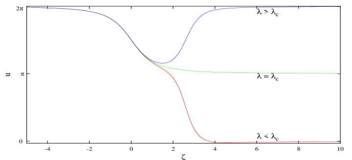
Figure 3: Solutions of Eq. (41), found numerically for $\lambda=2.63$ (upper curve), $\lambda=\lambda_{c}=2.62$ (middle curve), $\lambda=2.61$ (lower curve).

As $u$ represents the value of the field at the boundary ${\rm x}=0$ (cf. Eq. (14)), one concludes that the final state of the process at $\lambda<\lambda_{c}$ is the trivial vacuum, and no soliton production takes place. At the critical value, $\lambda=\lambda_{c}$, the function $u$ tends to $\pi$ when $\zeta\to+\infty$, and the solution describes the production of the sphaleron in the final state of the semiclassical evolution. Numerically we find

$$\lambda_{c}=2.62\;,$$ (43)

and the value of the corresponding energy is $E_{c}=1.2E_{S}$. Tunneling at the critical energy is still exponentially suppressed:

$$F(N=0,E=E_{c})=4\pi\mathop{\rm ln}\nolimits{\lambda_{c}}\;.$$

The picture we encounter here has been observed recently in quantum mechanics of two degrees of freedom [28] and in gauge theory [14]. Results obtained in both cases indicate that transitions at energies higher than critical proceed in two stages, creation of the sphaleron and its subsequent quantum decay into the relevant final state. The probability of the latter process is of order one, while the former is exponentially suppressed. The corresponding semiclassical solutions contain the sphaleron at $t\to+\infty$. In order to find such solutions one has to abandon the requirement of reality of the incoming wave $\phi_{i}$ on the real axis and thus the Ansatz (29).

4 Jumps onto sphaleron

4.1 Solutions with “zero” number of incoming particles

At energies higher than $E_{c}$ the Ansatz (29) is no longer applicable. Still, one can extract some information on the properties of $\phi_{i}$ from the analysis of Eqs. (15), (18). First, let us show that the singularity of $\phi_{i}$ situated inside the strip $\mathop{\rm Im}\nolimits z\in[0,T]$ is necessarily logarithmic. We denote the position of the singularity by $iT_{0}$. The function $\phi_{f}$ is regular at the point $z=iT_{0}$, so $\phi_{f}$ and $\phi_{f}^{\prime}$ can be replaced by constants in small vicinity of this point. Then, integration of Eq. (15) yields

$$\phi_{i}(z)=-f_{0}+2\mathop{\rm arctg}\nolimits\left[\frac{\sqrt{f_{1}^{2}-1}}{f_{1}}\mathop{\rm tg}\nolimits\left(\frac{\sqrt{f_{1}^{2}-1}}{2}(\mu z-C)\right)-\frac{1}{f_{1}}\right]~{},~{}~{}~{}~{}z\approx iT_{0}\;,$$ (44)

where $f_{0}=\phi_{f}(iT_{0})$, $f_{1}=\phi_{f}^{\prime}(iT_{0})/\mu$, and $C$ is the integration constant fixed by the condition that $z=iT_{0}$ is the singular point of the function $\phi_{i}$. One observes that the singularity of the expression (44) is logarithmic.

Thus the function $\phi_{i}$ has the form (30) with the function $R_{i}$ regular in the strip $\mathop{\rm Im}\nolimits z\in[0,T]$. Besides, one observes that conditions (31), (32) on $R_{i}$ are still valid, as their derivation does not make use of any particular Ansatz for $\phi_{i}$. Finally, due to Eq. (18), the presence of the logarithmic singularity of $\phi_{i}$ at $z=iT_{0}$ implies the existence of another singularity of $\phi_{i}$ with the structure

$$-ie^{-\theta}\mathop{\rm ln}\nolimits\left[\frac{\mu}{2}(z-i(2T-T_{0}))\right]\;.$$ (45)

This information enables one to cast the $T/\theta$ problem in the limit $\theta\to+\infty$ into the form suitable for numerical analysis. As already discussed, this limit is of primary interest as it corresponds to semiclassically vanishing number of incoming particles (this means that the real number of incoming particles is much smaller than $1/g^{2}$). We now proceed to the formulation of the corresponding equations.

According to Eq. (18), the function $\phi_{i}$ becomes regular in the half-plane $\mathop{\rm Im}\nolimits z>T$ when $e^{-\theta}$ tends to zero. As for its singularity in the strip $0<\mathop{\rm Im}\nolimits z<T$, it hits the line $\mathop{\rm Im}\nolimits z=T$ in the considered limit $\theta\to+\infty$, as is clear already from the general reasoning in Footnote 8. To demonstrate this explicitly, we write

$$\phi_{i}=i\mathop{\rm ln}\nolimits\left[\frac{\mu}{2}(z-iT_{0})\right]-ie^{-\theta}\mathop{\rm ln}\nolimits\left[\frac{\mu}{2}(z-i(2T-T_{0}))\right]+\tilde{R_{i}}(z)\;,$$ (46)

where $\tilde{R_{i}}(z)$ is regular both at $iT_{0}$ and $i(2T-T_{0})$. Equation (32) then implies

$$\frac{e^{-\theta}}{T-T_{0}}=-2\tilde{R_{i}}^{\prime}(iT_{0})\;.$$ (47)

This formula should be compared to Eqs. (38), (33) valid for the solutions below the critical energy. In that case $\tilde{R_{i}}^{\prime}(iT_{0})=-1/T\neq 0$. Let us assume that $\tilde{R_{i}}^{\prime}(iT_{0})\neq 0$ also for the solutions at energies above $E_{c}$. Then, Eq. (47) implies that $T_{0}$ indeed approaches $T$ when $e^{-\theta}\to 0$. We conclude that in the limit $\theta\to+\infty$ the function $\phi_{i}$ has the form

$$\phi_{i}=i\mathop{\rm ln}\nolimits\left[\frac{\mu}{2}(z-iT)\right]+\tilde{R_{i}}(z)\;,$$ (48)

where $\tilde{R_{i}}(z)$ is regular in the upper half-plane.

As in Sec. 3, it is convenient to consider equations for the functions $\phi_{i}$ and $\phi_{f}$ on the real axis $z=x\in\mathbb{R}$. Again, one should be careful about the asymptotics $x\to\pm\infty$. The function $\phi_{i}$ satisfies the condition (20). Taking into account the logarithmic cut of $\phi_{i}$ in the strip $0<\mathop{\rm Im}\nolimits z<T$ (cf. Sec. 3) and conditions (21), one obtains

$$\phi_{i}\to 2\pi,~{}~{}\phi_{f}\to 0~{}~{}~{}~{}~{}{\rm as}~{}~{}x\to-\infty\;,$$ (49a)

$$\phi_{i}\to 0,~{}~{}~{}\;\phi_{f}\to\pi~{}~{}~{}~{}~{}{\rm as}~{}~{}x\to+\infty\;.$$ (49b)

Note that the asymptotics of $\phi_{f}$ at $x=+\infty$ corresponds to the formation of the sphaleron at the end of the tunneling process.

A convenient expression for the action functional is obtained in the following way,

$$2\mathop{\rm Im}\nolimits S =2\mathop{\rm Im}\nolimits\int_{\cal C}dz(\phi_{f}\phi_{i}^{\prime}-\mu(1-\cos(\phi_{i}+\phi_{f})))$$

$$=-4\pi\mathop{\rm Im}\nolimits\tilde{R_{i}}(iT)+4\pi+2\mathop{\rm Im}\nolimits\int_{-\infty}^{\infty}dx(\phi_{f}\phi_{i}^{\prime}-\mu(1-\cos(\phi_{i}+\phi_{f})))\;.$$ (50)

In the second line we used Eq. (31) and took the limit $T_{0}\to T$. Integration in the last term is performed along the real axis; the first two terms account for the residue of the integrand in the logarithmic singularity of $\phi_{i}$. Finally, let us present convenient formulae for the energy of a solution. One finds two different expressions for the energies of the initial and final states; we denote these energies $E_{i}$ and $E_{f}$ respectively. For the final energy it is straightforward to obtain

$$E_{f}=2\mu+\int_{-\infty}^{\infty}dz(\phi_{f}^{\prime})^{2}\;,$$ (51)

where the first term is due to the presence of the sphaleron in the final field configuration. The analogous expression for the initial energy has the form

$$E_{i}=\int\limits_{-\infty+iT}^{+\infty+iT}dz(\phi_{i}^{\prime})^{2}\;.$$ (52)

In the limit $e^{-\theta}\ll 1$ the integral in (52) is saturated by the contribution of the singularity at $z=i(2T-T_{0})$. One obtains

$$E_{i}=2\pi\frac{e^{-\theta}}{T-T_{0}}=-4\pi\tilde{R_{i}^{\prime}}(iT)\;,$$ (53)

where in the second equality we used Eq. (47).

We have performed numerical solution of the following set of equations formulated on the real axis: differential equation (15) with the boundary conditions (49), condition of reality of $\phi_{f}$ (Eq. (16)) and analyticity condition (48). Details of our numerical method are presented in Appendix C. Let us mention here an interesting property of the solutions. One notes that the above set of equations is invariant under the transformation

$$\phi_{i}(z)\mapsto 2\pi-\big{(}\phi_{i}(-z^{*})\big{)}^{*}\;,$$ (54a)

$$\phi_{f}(z)\mapsto\pi-\big{(}\phi_{f}(-z^{*})\big{)}^{*}\;.$$ (54b)

We find that the tunneling solutions at $E>E_{c}$ are symmetric with respect to this transformation. This property distinguishes them from the solutions at energies lower than critical.

The imaginary part of the action, the energy and suppression exponent are calculated according to formulae (50), (51), (53); we use the equality of the initial and final energies as a cross–check of the precision of numerical calculations. Results for the suppression exponent $F(N=0)$ are presented in Fig. 1. They cover the interval $E_{c}<E<2.3E_{S}$ of the region II. Let us stress that our numerical solutions describe tunneling with exactly zero semiclassical number of incoming particles. The fact that one is able to find such solutions is a peculiarity of the model. Unlike in the case of more complicated systems [14] we do not need to perform calculations at finite $N$.

At energies higher than $2.3E_{S}$ the numerical analysis with the method outlined in this subsection becomes problematic. The point is that with the growth of energy, the parameter $T$ decreases, and the logarithmic singularity of the solution approaches the real axis, according to Eq. (48). Hence, the finite–difference approximation used in numerical calculations breaks down in the region near $z=0$ at small $T$. Luckily, as we show in the next subsection, at $\mu T\ll 1$ the singularity can be isolated and treated analytically, thus allowing for complete determination of the solution in the limit $T\to 0$. The energy and suppression exponent of the limiting solution yield the point $(E_{l},F(E_{l}))$ of the graph in Fig. 1. The interval of energies between $2.3E_{S}$ and $E_{l}$ is covered by expanding the solution at these energies in powers of the small parameter $\mu T$ around the limiting solution, see Appendix D.

4.2 Limit $T\to 0$

In this subsection we determine the tunneling solution in the limit $T\to 0$. We will have to resolve the structure of the singularity of the solution in the region near the point $z=0$, so we keep $T$ small but non-zero, $\mu T\ll 1$, and take the limit only in the final formulae for the energy and suppression exponent. For the same purpose we introduce small but non-vanishing $e^{-\theta}\ll 1$. It is convenient to choose the contour ${\cal C}$, entering the formula (22) for the action functional, as shown in Fig. 4. From Eqs. (20), (21) one obtains that the asymptotics of the solution on the left part of the contour ${\cal C}$ is given by

$$\phi_{i}\to 0,~{}~{}\phi_{f}\to 0~{},~{}~{}~{}{\rm at}~{}~{}x\to-\infty\;,$$ (55)

while Eq. (49b) remains intact. The difference between Eq. (55) and Eq. (49a) is explained by the fact that the contour ${\cal C}$ and the real axis lie on different sides of the logarithmic cut of the function $\phi_{i}$. Correspondingly, the symmetry of solutions considered along the contour ${\cal C}$ is slightly different from (54): instead of (54a) one has

$$\phi_{i}(z)\mapsto-\phi_{i}^{*}(-z^{*})\;.$$ (56)

We search for solutions invariant under the transformation (56), (54b).

Let us introduce $\varepsilon={\rm max}\{T,e^{-\theta}/\mu\}$. Our strategy is to separate the complex plane into “hard” ($|z|\ll 1/\mu$) and “soft” ($|z|\gg\varepsilon$) regions, solve equations separately in these regions and glue solutions in their intersection $\varepsilon\ll|z|\ll 1/\mu$, see Fig. 4.

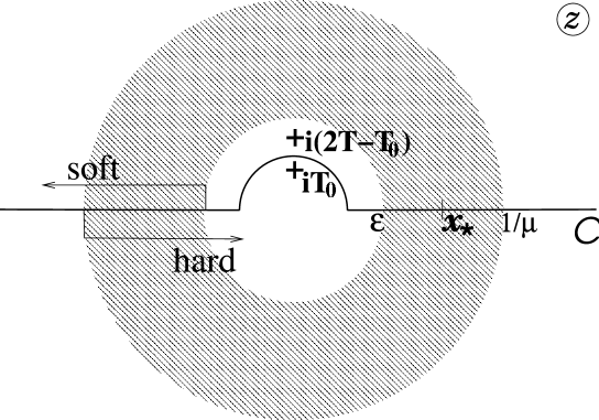
Figure 4: “Hard” and “soft” regions of the complex plane; respective pieces of solution are glued together in the shaded area. Crosses represent the singularities of the function $\phi_{i}$ in the upper half–plane.

Let us start with the “hard” region. Inserting the expression (30) for $\phi_{i}$ into Eq. (15) and neglecting terms of order $O\big{(}(\mu z)^{2}\big{)}$, one obtains

$$R_{i}^{\prime}-\phi_{f}^{\prime}=-\frac{i}{z-iT_{0}}\left(1+e^{i(R_{i}+\phi_{f})}\right)\;.$$ (57)

An obvious solution to this equation is

$$R_{i}=\phi_{f}=\frac{\pi}{2}\;.$$ (58)

The corresponding function $\phi_{i}$ satisfies the $\theta$-condition (18) to the zeroth order in $e^{-\theta}$. However, we saw in Sec. 4.1 that in this approximation the solution is singular on the contour ${\cal C}$ (cf. Eq. (47)). So we need to find the regularized solution which satisfies the $\theta$-conditions to the first order in $e^{-\theta}$. To this end, we linearize Eq. (57):

$$r^{\prime}-\varphi^{\prime}=-\frac{r+\varphi}{z-iT_{0}}\;.$$ (59)

Here notations $r=R_{i}-\pi/2$, $\varphi=\phi_{f}-\pi/2$ are introduced. Equation (59) can be solved with respect to any of the two functions, $\varphi$ or $r$. One gets

$$\varphi=-r+(z-iT_{0})\int^{z}\frac{2r^{\prime}(z_{1})}{z_{1}-iT_{0}}dz_{1}\;,$$ (60)

$$r=\varphi-\frac{2}{z-iT_{0}}\int_{iT_{0}}^{z}\varphi(z_{1})dz_{1}\;,$$ (61)

where the integration constant in the expression (61) is chosen in such a way that the function $r$ is regular at the point $z=iT_{0}$. We do not specify the value of the integration constant in Eq. (60) as this constant is irrelevant for what follows.

Let us investigate the singularities of the functions $\varphi$, $r$. In the same way as in the previous subsection, one observes that the only singularity of $r$ in the upper half-plane is situated at $z=i(2T-T_{0})$ and has the form (45) (cf. Eq. (46)). Then, it follows from Eq. (60) that the only singularity of $\varphi(z)$ in the upper half-plane is situated at the same point, $z=i(2T-T_{0})$ (an apparent singularity at $z=iT_{0}$ is eliminated, as before, by imposing condition (32) on the function $r$). Reality of $\varphi$ on the real axis implies now that the only other singularity of $\varphi$ is situated at the point $z=-i(2T-T_{0})$, its structure being “complex conjugate” to that of the singularity at $z=i(2T-T_{0})$. We determine the form of these singularities from Eq. (60), single them out explicitly and expand the remaining entire function into power series. In this way we get the following representation:

$$\varphi= -\frac{e^{-\theta}}{\mu(T-T_{0})}\left(\mu(z-iT)\mathop{\rm ln}\nolimits\left[\frac{\mu}{2}(z-i(2T-T_{0}))\right]+\mu(z+iT)\mathop{\rm ln}\nolimits\left[\frac{\mu}{2}(z+i(2T-T_{0}))\right]\right)$$

$$-\frac{\pi Te^{-\theta}}{T-T_{0}}+A_{0}\mu z+\sum_{n=1}^{\infty}A_{n}(\mu z)^{1+2n}\;.$$ (62)

The first term in the second line as well as the presence of only odd powers in the power series are fixed by the symmetry (54b). The coefficients in Eq. (62) are to be determined by matching this expression to the solution in the “soft” region. We will see below that the function $\phi_{f}$ in the latter region is of order one, and thus all the coefficients, $\frac{e^{-\theta}}{\mu(T-T_{0})}$, $A_{0}$, $A_{n}$ are of order one. So, the contribution of the sum in Eq. (62) can be neglected in the “hard” domain; we omit it in what follows. Inserting expression (62) into Eq. (61) one gets:

$$\begin{split}r=&-ie^{-\theta}\mathop{\rm ln}\nolimits\left[\frac{\mu}{2}(z-i(2T-T_{0}))\right]+i\frac{T+T_{0}}{T-T_{0}}e^{-\theta}\mathop{\rm ln}\nolimits\left[\frac{\mu}{2}(z+i(2T-T_{0}))\right]\\ &-\frac{4TT_{0}}{T-T_{0}}e^{-\theta}\frac{1}{z-iT_{0}}\mathop{\rm ln}\nolimits\left[1+\frac{z-iT_{0}}{2iT}\right]-\frac{e^{-\theta}}{T-T_{0}}(z+iT_{0})+\frac{\pi Te^{-\theta}}{T-T_{0}}-iA_{0}\mu T_{0}\;.\end{split}$$ (63)

In the region $\varepsilon\ll|z|\ll 1/\mu$ the expressions (62), (63) simplify. In terms of the original functions $\phi_{i}$, $\phi_{f}$, one obtains

$$\phi_{i}=i\mathop{\rm ln}\nolimits\left[\frac{\mu}{2}(z-i0)\right]+\frac{\pi}{2}-\frac{e^{-\theta}}{T-T_{0}}\;z~{},~{}~{}~{}~{}~{}~{}~{}\phi_{f}=\frac{\pi}{2}-\frac{e^{-\theta}}{T-T_{0}}\;z\mathop{\rm ln}\nolimits\left(\frac{\mu^{2}z^{2}}{4}\right)+A_{0}\mu z\;,$$ (64)

where terms of order $O(\mu T)$, $O(e^{-\theta})$, $O\big{(}(\mu z)^{2}\big{)}$ have been neglected.

We now turn to the “soft” region. Here the contour ${\cal C}$ coincides with the real axis. Introducing the real and imaginary parts of the incoming wave, $\phi_{i}(x)=a(x)+ib(x)$, one rewrites Eq. (15) as a set of two real equations,

$$b^{\prime}=\mu\mathop{\rm sh}\nolimits{b}\cos{u}\;,$$ (65)

$$u^{\prime}=2a^{\prime}-\mu\mathop{\rm ch}\nolimits{b}\sin{u}\;,$$ (66)

where $u(x)=a(x)+\phi_{f}(x)$. In the “soft” region one can neglect the regularizing parameters $\mu T$, $e^{-\theta}$. [Solutions at non-zero $T$ are considered in Appendix D.] Then, the function $\phi_{i}$ is regular in the upper half-plane of the “soft” region, and the derivatives of its real and imaginary parts are related by an analog of the Cauchy formula,

$$a^{\prime}(x)=\frac{1}{\pi x}{\rm V.P.}\!\!\int_{-\infty}^{\infty}dx_{1}\frac{x_{1}b^{\prime}(x_{1})}{x_{1}-x}\;,$$ (67)

where the integral is understood in the sense of principal value. Equations (65), (66), (67) are supplemented by boundary conditions at $x=0$ which originate from matching with the “hard” part of solution. From the expressions (64) one obtains

$$b\to\mathop{\rm ln}\nolimits{\left(\frac{\mu}{2}x\right)}~{},~{}~{}~{}a\to\frac{\pi}{2}~{},~{}~{}~{}u\to\pi~{},~{}~{}~{}~{}{\rm at}~{}~{}~{}x\to+0\;.$$ (68)

The conditions at $x\to-0$ can be reconstructed from the requirement of symmetry with respect to (56), (54b). For completeness we write down the boundary conditions (49b), (55) explicitly:

$$a\to 0~{},~{}~{}~{}~{}b\to 0~{},~{}~{}~{}u\to\pi~{},~{}~{}~{}~{}~{}{\rm at}~{}~{}x\to+\infty\;,$$ (69)

while the symmetry transformations (54b), (56) are:

$$b(x)\mapsto b(-x)~{},~{}~{}~{}a(x)\mapsto-a(-x)~{},~{}~{}~{}u(x)\mapsto\pi-u(-x)\;.$$ (70)

Due to the symmetry (70), it is sufficient to consider half of the real axis, and we assume $x>0$ in what follows. Given the function $u$, equation (65) can be integrated explicitly:

$$b(x)=\mathop{\rm ln}\nolimits{\mathop{\rm th}\nolimits\left(-\frac{\mu}{2}\int_{0}^{x}\cos{u(x_{1})}dx_{1}\right)}\;,$$ (71)

where the condition (68) is imposed on $b(x)$ at the origin. Equations (71), (67), (66) form a complete system.

One obtains a fairly good approximation by linearizing Eqs. (71), (66) with respect to $\delta u=u-\pi$. Equation (71) takes the form

$$b=\mathop{\rm ln}\nolimits{\mathop{\rm th}\nolimits{\left(\frac{\mu}{2}x\right)}}\;.$$

Substitution of this expression into Eq. (67) yields

$$a^{\prime}=-\frac{\mu}{\pi}\left(\beta\left(1+i\frac{\mu}{\pi}x\right)+\beta\left(1-i\frac{\mu}{\pi}x\right)\right)\;,$$

where

$$\beta(x)=\frac{d}{dx}\left(\mathop{\rm ln}\nolimits{\left[\Gamma\left(\frac{x+1}{2}\right)\right]}-\mathop{\rm ln}\nolimits{\left[\Gamma\left(\frac{x}{2}\right)\right]}\right)\;.$$

Now, $\delta u$ can be found from Eq. (66). The corresponding analytic expression is not illuminating, and we do not present it here. The linear approximation is improved by numerical iterations. Each cycle consists of solving Eqs. (71), (67), (66) thus determining functions $b$, $a$, $\delta u$ one after another, starting from the approximation for $\delta u$ obtained in the previous cycle. After $30$ iterations one obtains numerical solution with precision of order $10^{-6}$. The resulting functions $a$, $b$, $\delta u$ together with those obtained in the linear approximation are plotted in Fig. 5.

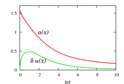
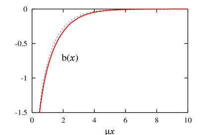
Figure 5: Limiting solution in the “soft” region. Dashed lines represent linear approximation in $\delta u$.

Let us consider the behavior of the solution at $x\to+0$. Equation (66) allows for the following behavior:

$$a=\frac{\pi}{2}-A\mu x+O(x^{2})~{},~{}~{}~{}~{}~{}~{}~{}\phi_{f}=\frac{\pi}{2}-2A\mu x\mathop{\rm ln}\nolimits{\left(\frac{\mu x}{2}\right)}+B\mu x+O(x^{2})\;.$$ (72)

We observe that both the solution in the linear approximation and the full numerical solution exhibit this behaviour. Numerically, $A=0.845$, $B=-2.90$. Matching these expressions to the asymptotics (64) of the “hard” part of the solution, one obtains

$$\frac{e^{-\theta}}{T-T_{0}}=A\mu~{},~{}~{}~{}A_{0}=B\;.$$ (73)

Thus, the limiting solution is completely determined.

A comment is in order. Strictly speaking, in the limit $T,e^{-\theta}\to 0$ the “soft” region covers the whole complex plane and one is left with the “soft” part of the solution only. However, the solution is then singular at $z=0$, and it is impossible to calculate its energy and action. So the term “limiting solution” implies not only the form of the solution in the “soft” region but also the appropriate resolution of the singularity, Eqs. (62), (63).

The next step is to evaluate the imaginary part of the action functional on the constructed solution. It is natural to separate it into the sum of contributions of the “hard” and “soft” regions. Neglecting terms of order $\mu T$, $e^{-\theta}$ we have

$$2\mathop{\rm Im}\nolimits S_{hard}=2\mathop{\rm Im}\nolimits\int\limits_{C,|z|<x_{*}}\left(\frac{i\pi}{2(z-iT_{0})}-\mu-\frac{1}{z-iT_{0}}\right)~{}dz=2\pi\;.$$

Here $x_{*}$ is some number in the range $\varepsilon\ll x_{*}\ll 1/\mu$. For the “soft” contribution we write

$$\begin{split}2\mathop{\rm Im}\nolimits S_{soft}&=2\int_{|x|>x_{*}}(\phi_{f}b^{\prime}-\mu\mathop{\rm sh}\nolimits{b}\sin{u})~{}dx\\ &=2\pi b(x_{*})+4\int_{x_{*}}^{\infty}(\phi_{f}-\mathop{\rm tg}\nolimits{u})b^{\prime}~{}dx=4\int_{0}^{\infty}\left(\frac{u^{\prime}}{\cos^{2}u}-\phi_{f}^{\prime}\right)b~{}dx\;,\end{split}$$ (74)

where in passing from the first to the second line we used Eq. (65) and symmetry with respect to (70), while in the last expression terms vanishing in the limit $x_{*}\to 0$ are neglected. A good estimate for $2\mathop{\rm Im}\nolimits S_{soft}$ is obtained in the linear approximation:

$$2\mathop{\rm Im}\nolimits S_{soft}^{lin}=4\int_{0}^{\infty}a^{\prime}b~{}dx=4\pi\left(-6\zeta^{\prime}(-1)-\frac{\mathop{\rm ln}\nolimits{2}}{6}-\frac{\mathop{\rm ln}\nolimits{\pi}}{2}\right)=3.83\;,$$

where integration is performed using Eqs. 8.371.2, 3.951.14 from Ref. [32]. The calculation of the integral (74) for the full numerical solution yields $2\mathop{\rm Im}\nolimits S_{soft}=3.98$. Note that this value is comparable to the contribution $2\pi$ coming from the “hard” core.

An important quantity is the energy of the limiting solution. Again, we calculate separately the energies of the initial and final states. While formula (51) for the final energy is directly applicable in the limit $T\to 0$, the analog of Eq. (53) for the initial energy is

$$E_{i}=2\pi\frac{e^{-\theta}}{T-T_{0}}=2\pi A\mu\;,$$

where $A$ is defined in Eqs. (72). For our numerical solution $E_{f}=E_{i}$ with good accuracy, this may be viewed as a confirmation of the consistency of the numerical method; the obtained value is

$$E_{l}=2.65E_{S}\;.$$ (75)

At first sight, the result (75) is puzzling. Indeed, one could expect to cover the whole range of energies up to infinity by sending the parameter $T$ to zero. However from Eq. (75) we learn that this is not the case: $T/\theta$-problem does not have any solutions with energies higher than $E_{l}$. On the other hand, the suppression exponent is still non-vanishing at the limiting energy,

$$F(N=0,E=E_{l})=10.27\;.$$ (76)

A question is then, how tunneling occurs at energies above $E_{l}$, and what is the corresponding tunneling probability.

The answer is suggested by an observation that in all the formulae describing the limiting solution, even in those related to the “hard” core, one can set $T=0$ (it is sufficient to keep $e^{-\theta}$ non-zero to resolve the singularity of the solution). As discussed at the end of Sec. 2.1, the solution obtained in this way belongs to the class of real–time instantons. Thus, it gives the maximum probability for tunneling from states with semiclassically vanishing number of particles. Consequently, the suppression exponent $F(N=0,E>E_{l})$ is not smaller than $F(N=0,E=E_{l})$. It cannot be larger either, because one can always imagine a tunneling process which has the same exponential suppression as the process at the limiting energy. Namely, incoming particle(s) can release the energy excess $(E-E_{l})$ by the perturbative emission of a few other particles at the beginning of the process, so that subsequent tunneling occurs effectively at the energy $E_{l}$. From this physical reasoning one concludes that the suppression exponent stays constant at energies higher than $E_{l}$ (cf. Ref. [15]). Remarkably, the semiclassical treatment is still possible at these energies. We return to this issue in Sec. 4.4. Now, let us turn to the real–time instantons which, for their novelty, deserve a somewhat detailed study.

4.3 Real-time instantons

Let us recall that the real-time instantons are solutions of the $T/\theta$-problem with $T=0$ and finite $\theta$. In the model under consideration these solutions can be obtained by an iterative method which is a slight modification of that used in the previous subsection. As before, one introduces the functions $a$, $b$, $u$ satisfying Eqs. (65), (66). Note that, unlike in the case of Sec. 4.2, all the functions are supposed to be regular on the entire real axis, including the point $x=0$.

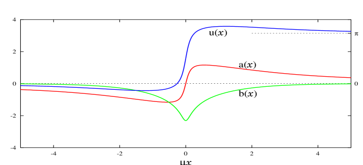
Figure 6: Example of real-time instanton configuration with $\theta=2.04$, $N=2.3$.

Requirements of regularity together with symmetry under the transformations (70) lead to the following conditions at $x=0$,

$$b^{\prime}(0)=0~{},~{}~{}~{}a(0)=0~{},~{}~{}~{}u(0)=\pi/2\;.$$ (77)

Formula (67) is not directly applicable in the case of finite $\theta$. An appropriate modification comes about when one notices that a direct analog of Eq. (67) relates the real $\tilde{a}$ and imaginary $\tilde{b}$ parts of the function $\chi$ introduced in Eqs. (18), (19). Using Eq. (18), one expresses the functions $a$, $b$ in terms of $\tilde{a}$, $\tilde{b}$ and gets, instead of Eq. (67),

$$a^{\prime}(x)=\frac{1+e^{-\theta}}{1-e^{-\theta}}\cdot\frac{1}{\pi x}{\rm V.P.}\!\!\int_{-\infty}^{\infty}dx_{1}\frac{x_{1}b^{\prime}(x_{1})}{x_{1}-x}\;.$$ (78)

Finally, Eq. (65) can be integrated explicitly in the present case as well, but now the integration constant is arbitrary,

$$b(x)=\mathop{\rm ln}\nolimits{\mathop{\rm th}\nolimits\left(-\frac{\mu}{2}\int_{0}^{x}\cos{u(x_{1})}dx_{1}+\varkappa\right)}\;.$$ (79)

We obtain numerical solutions by iterating Eqs. (79), (78), (66) in the indicated order. The value of $\varkappa$ is determined at each cycle of iterations from the requirement that the function $u$ satisfies the boundary conditions (77), (69). An example of real–time instanton configuration is shown in Fig. 6.

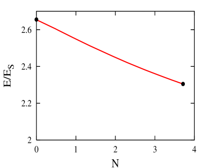
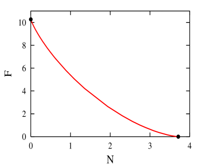
Figure 7: Energy and suppression exponent versus the number of incoming particles in the case of real-time instantons.

It is straightforward to obtain the energy and imaginary part of the action from Eqs. (51) and (22). As for the number of incoming particles, in the case of real–time instantons it can be expressed in a particularly convenient form,

$$N=-\frac{2}{\mathop{\rm sh}\nolimits{\theta}}\int_{-\infty}^{+\infty}a^{\prime}b~{}dx\;,$$

which can be obtained from Eq. (8b) in a straightforward way. The energy and suppression exponent as functions of the initial number of particles are shown in Fig. 7. The curves start at $N=0$ from the values corresponding to the limiting solution and end up at $N=3.7$ where the suppression exponent is zero. We see that the branch of real-time instantons interpolates between the limiting solution and the region of classically allowed transitions.

4.4 Tunneling above the limiting energy

In this subsection we follow an approach which is somewhat different from that used in the rest of the paper. Instead of considering the inclusive probability (5), we study tunneling from a single initial state with given number of particles $N$ and energy $E$. The energy is assumed to be higher than the energy of the real–time instanton corresponding to the same initial number of particles, $E>E^{(rt)}(N)$. Let us demonstrate that the suppression exponent of tunneling from an appropriately chosen initial state coincides with that of the real–time instanton.

Using the approach of Ref. [33], one can show that any field configuration which satisfies Eqs. (7a), (7b), (7c) (but not necessarily Eq. (7e)) in the complex time plane determines the suppression exponent for the tunneling probability of the form

$$\tilde{\cal P}(E,N;a)=\sum_{f}\frac{|\langle f|\hat{\cal S}\hat{P}_{E}\hat{P}_{N}|a\rangle|^{2}}{\langle a|\hat{P}_{E}\hat{P}_{N}|a\rangle}\;.$$ (80)

Here summation is performed over the final states only, the initial state $\hat{P}_{E}\hat{P}_{N}|a\rangle$ is a coherent state projected onto the subspace with fixed energy and number of particles. The coherent state corresponding to a given solution is defined by

$$\hat{a}_{k}|a\rangle=f_{k}|a\rangle\;,$$ (81)

where $f_{k}$ are the positive frequency components of the solution $\phi(t,{\rm x})$ at $t\to-\infty$,

$$\phi(t,{\rm x})\Big{|}_{t\to-\infty}=\frac{1}{(2\pi)^{1/2}}\int\frac{dk}{\sqrt{2\omega_{k}}}\left(f_{k}\mathrm{e}^{-i\omega_{k}t+ik{\rm x}}+g_{k}^{*}\mathrm{e}^{i\omega_{k}t-ik{\rm x}}\right)\;.$$

Note that unlike in Eq. (7d) we now consider the asymptotics along the real $t$-axis. The suppression exponent for the probability (80) is still given by Eq. (11) where the parameters $T$ and $\theta$ are now determined from the following equations,

$$E=\int dk\omega_{k}f_{k}f_{k}^{*}{\rm e}^{2\omega_{k}T+\theta}~{},~{}~{}~{}~{}N=\int dkf_{k}f_{k}^{*}{\rm e}^{2\omega_{k}T+\theta}\;.$$ (82)

One can check that, as before, $E$ coincides with the actual energy of the solution, and the expressions (8) for the energy and number of incoming particles are applicable. Note that in general the average energy and number of particles in the state $|a\rangle$ are different from $E$ and $N$.

We consider the following configurations which differ from the real–time instanton by a small perturbation:

$$\phi_{i,f}(z)=\phi_{i,f}^{(rt)}(z)+\alpha\psi(z/\beta)\;,\\$$ (83)

where the perturbation is represented by the function $\psi(z)$ which is real on the real axis and falls off fast enough at $x\to\pm\infty$. When the parameters $\alpha$, $\beta$ are small, $\beta\ll\alpha\ll 1$, the configuration (83) is an approximate solution of Eq. (15). Evaluation of the energy and number of incoming particles using Eqs. (51), (8b) yields

$$E=E^{(rt)}+\frac{\alpha^{2}}{\beta}\int dx(\psi^{\prime}(x))^{2}+O(\alpha)\;,$$

$$N=N^{(rt)}+O(\alpha^{2})\;.$$

These formulae demonstrate that in the limit

$$\alpha,\beta\to 0~{},~{}~{}~{}~{}\alpha^{2}/\beta~{}~{}{\rm fixed}$$

the solution (83) describes tunneling from a state which differs from the initial state of the real–time instanton by addition of a few particles carrying a finite amount of energy. Comparison of the structure of the initial and final waves shows that these particles scatter elastically from the boundary ${\rm x}=0$ and do not affect the tunneling process. It is straightforward to evaluate the imaginary part of the action of the solution (83) and determine the parameters $T$ and $\theta$ from the formulae (82). In this way one finds that the suppression exponent of the solution (83) coincides with that of the real–time instanton up to terms $O(\alpha)$.

As before, the suppression exponent of collision–induced tunneling is obtained in the limit $N\to 0$. One concludes that it is equal to that of the limiting solution at all energies above $E_{l}$.

5 Concluding remarks

The results obtained in this paper show that in the model (1) the soliton production due to collision of a particle with the boundary is always exponentially suppressed. This may be viewed as an evidence in favour of the exponential suppression of collision–induced tunneling at all energies in other theories. We have identified the mechanism of suppression at high energies of colliding particles. It is a consequence of substantial rearrangement the system has to undergo in the course of transition. Moreover, this rearrangement occurs in an optimal way at a certain limiting energy $E_{l}$ where the suppression is the weakest. At higher energies the system emits the excess of energy in the form of particles which do not interfere with the tunneling process, and subsequent transition occurs with the energy $E_{l}$. The consequence of the latter phenomenon is that the suppression exponent stays constant all the way from $E=E_{l}$ to $E=\infty$. It is natural to conjecture that this mechanism of suppression is generic for collision–induced tunneling in quantum field theory.

As a by-product we have found that there is a novel type of tunneling configurations which we call real–time instantons. These are solutions to the $T/\theta$-problem with the parameter $T$ set equal to zero. From the physical point of view, real–time instantons provide maximum probability for tunneling from initial states with given number $N$ of incoming particles. In the plane of parameters $(E,N)$, the line of real–time instantons interpolates between the region of classically allowed transitions and the point $(E=E_{l},N=0)$. The suppression exponent calculated for a real–time instanton $F_{rt}(N)$ sets a lower bound on the suppression exponent $F(E)$ for the tunneling induced by one or a few incoming particles at all energies. Modulo standard assumptions, $F_{rt}(N)$ in the limit $N\to 0$ coincides with $F(E)$ at energies higher than $E_{l}$. Thus, one can use real–time instantons to determine the value of the limiting energy $E_{l}$ and the suppression exponent of collision–induced tunneling at energies higher than $E_{l}$ in various models.

Finally, let us recall that the model investigated in this paper describes various condensed matter systems. It would be interesting to work out implications of our results for these systems.

Acknowledgements

We are indebted to S. Dubovsky for bringing to our attention the model considered in this paper and for collaboration at early stage of the work. We thank V. Rubakov and F. Bezrukov for their encouraging interest and helpful suggestions. We are grateful to S. Demidov, D. Gorbunov, M. Libanov, E. Nugaev, C. Rebbi, A. Ringwald, G. Rubtsov, S. Troitsky for fruitful discussions. This work has been supported in part by Russian Foundation for Basic Research, grant 02-02-17398, grant of the President of Russian Federation NS-2184.2003.2 and personal felloships of the “Dynasty” foundation (awarded by the Scientific board of ICFPM). The work of D. L. has been supported by CRDF award RP1-2364-MO-02 and INTAS grant YS 03-55-2362. S. S. is grateful to DESY Theory group in Hamburg for hospitatlity during his visit.

Appendix A Periodic instantons at non-zero bulk mass

Let us consider the effect of non-zero bulk mass $m$ on the periodic instantons found in Sec. 3.1. We assume that the mass is small, $mT\ll 1$. An approximate periodic instanton $\phi_{m}(t,{\rm x})$ in the massive case is constructed in the following way. In the region $|t|\ll 1/m$, one has

$$\phi_{m}(t,{\rm x})=\phi_{0}(t,{\rm x}){\rm e}^{-m{\rm x}}\;,$$ (84)

where $\phi_{0}(t,{\rm x})$ is the periodic instanton solution in the massless case given by Eqs. (14), (25). It is straightforward to check that the configuration (84) satisfies the field equations (7a), (7b) up to terms of order $O(mT)$. At $|t|\gg T$ the value of the field at the boundary is frozen to $0$ and $2\pi$ in the parts $A$ and $D$ of the contour $ABCD$, respectively (see Fig. 2). Let us concentrate on the initial part of the contour; we set $t=t^{\prime}+iT$. In the region $T\ll|t^{\prime}|\ll 1/m$, the configuration (84) should be matched to the solution of the free massive equation, which has the form (7d). Making use of Eq. (28), one obtains the Fourier transform of the function $\phi_{m}$:

$$\phi_{m}(t^{\prime},{\rm x})=\int_{-\infty}^{\infty}\frac{dk}{k-im}\cdot\frac{-i{\rm e}^{ikx_{0}}}{2\mathop{\rm ch}\nolimits\left(\frac{kT}{2}\right)}{\rm e}^{ik(t^{\prime}+{\rm x})}~{}~{},~{}~{}~{}~{}~{}~{}T\ll|t^{\prime}|\ll\frac{1}{m}\;,$$

where we omitted terms negligible in the limit $m\to 0$. Comparing this expression to Eq. (7d) we get,

$$f_{k}=\theta(-k)\frac{-i\sqrt{\pi\omega_{k}}{\rm e}^{ikx_{0}}}{(k-im)\;\mathop{\rm ch}\nolimits\left(\frac{kT}{2}\right)}\;,$$

$$g^{*}_{k}=\theta(-k)\frac{-i\sqrt{\pi\omega_{k}}{\rm e}^{-ikx_{0}}}{(-k-im)\;\mathop{\rm ch}\nolimits\left(\frac{kT}{2}\right)}\;.$$

Now, it is straightforward to evaluate the energy and the number of incoming particles using Eqs. (8). The energy is given by the same formula as in the massless case, Eq. (26), while the initial number of particles is

$$N=\int_{0}^{\infty}\frac{\pi}{\sqrt{k^{2}+m^{2}}\;\mathop{\rm ch}\nolimits^{2}\!\!\left(\frac{kT}{2}\right)}dk=-\pi\mathop{\rm ln}\nolimits(mT)+O(1)\;.$$

We see that the small bulk mass does not affect the energy of the periodic instanton. On the other hand, it regularizes the number of incoming particles which diverges logarithmically in the limit $m\to 0$. To find the effect of the mass on the value of the action, one performs integration by parts in expression (10) and obtains

$$S=\int dt\left.\left(\frac{1}{2}\phi\partial_{\rm x}\phi-\mu(1-\cos{\phi})\right)\right|_{{\rm x}=0}\;.$$

From the above consideration it follows that the integrand is non-vanishing only at $t\sim T\ll 1/m$. So, one substitutes the expression (84) into this formula and finds that the value of the action differs from that in the massles case by terms of order $O(mT)$. We conclude that the influence of the small mass on the suppression exponent of tunneling described by the periodic instanton is small when the energy of the process is much higher than the mass.

Appendix B Analytic proof of existence of the critical energy

We are going to prove the following statements concerning Eq. (41):
a) if $\lambda>4$, a solution of Eq. (41) with asymptotics (42) exists;
b) if $\lambda<\pi/2$, there is no solution of Eq. (41) with asymptotics (42).

We start with the statement (a). At $\lambda>4$ the lines defined by equation

$$\frac{4}{1+\zeta^{2}}+\lambda\sin{u}=0$$ (85)

separate the band $\pi<u<2\pi$ of the $(\zeta,u)$ plane into three regions, where the derivative of solution of Eq. (41) has different signs, see Fig.8.

Figure 8: Regions of positive and negative $u^{\prime}$ and qualitative form of the solution of Eq.(41) in the case $\lambda>4$.

The condition (42a) picks up a single solution of Eq.(41). The integral curve of this solution starts from the region I at $\zeta=-\infty$. As $\zeta$ increases, it crosses the line $u^{\prime}=0$ and comes into the region II where $u^{\prime}>0$. Once in the region II, the integral curve cannot leave it. Thus, $u^{\prime}$ stays positive all the way to $\zeta=+\infty$, and the integral curve gets attracted to the asymptotics $2\pi$ when $\zeta\to+\infty$.

We now proceed to the proof of the statement (b). At $\lambda<\pi/2$, the form of the lines (85) is different, see Fig. 9. The tips of these lines are situated at $\zeta=\pm\zeta_{0}$, where

$$\zeta_{0}=\sqrt{4/\lambda-1}\;.$$

At $\zeta<-\zeta_{0}$ the integral curve of the solution lies in the region I where $u^{\prime}<0$.

Figure 9: Regions of positive and negative $u^{\prime}$ and qualitative form of the solution of Eq.(41) in the case $\lambda<\pi/2$.

Let us show that it crosses the line $u=\pi$ from above within the interval $-\zeta_{0}<\zeta<\zeta_{0}$. Indeed, Eq. (41) implies,

$$u^{\prime}\leq\lambda-\frac{4}{1+\zeta^{2}}\;.$$

Integration of the latter inequality yields

$$u(\zeta_{0})\leq u(-\zeta_{0})+2\lambda\zeta_{0}-8\mathop{\rm arctg}\nolimits{\zeta_{0}}<\pi\;.$$

Once the integral curve comes below the line $u=\pi$, it cannot reach the region II where $u^{\prime}>0$ (see Fig. 9). Thus it does not approach the asymptotics $2\pi$ at $\zeta\to+\infty$.

The above analysis necessitates the existence of the critical value $\pi/2<\lambda_{c}<4$ at which the behavior of the solution changes qualitatively. We have obtained the value of $\lambda_{c}$ numerically, see Eq. (43).

Appendix C Numerical method at $E>E_{c}$

In this Appendix we formulate a discretized version of the problem (15), (16), (48), (49). When searching for an appropriate numerical method, one encounters two major difficulties. First, since all the relevant solutions at $E>E_{c}$ are close to the sphaleron configuration at $t\to+\infty$, they display an instability similar to that of the sphaleron. To overcome this difficulty, we use specifics of the system in hand. As already mentioned, equations (15), (16), (48) and boundary conditions (49) are invariant under the transformation (54). So, it is natural to look for solutions symmetric with respect to this transformation. Once the symmetry requirement is imposed, the set of considered configurations is restricted to those close to the sphaleron at $t\to+\infty$, and solutions become stable.

The second numerical challenge is the slow falloff of the solutions at $x\to\pm\infty$. Equation (15) allows for solutions with asymptotic behavior $1/x$ at $x\to\pm\infty$, and numerical analysis confirms that this is indeed the case. We overcome this problem by introducing a non–uniform lattice with link size growing when $x\to\pm\infty$. This is achieved by performing conformal transformation of the complex $z$–plane,

$$w=\frac{z-iT}{z+iT}\;,$$ (86)

which maps the real axis onto the the unit circle $w=\mathrm{e}^{i\alpha}$. In particular, the asymptotic regions $x\to-\infty$ and $x\to+\infty$ correspond to the vicinities of the points $\alpha=0$ and $\alpha=2\pi$, respectively. It is clear that the uniform lattice in angle $\alpha$ produces discretization of the required type of the real $z$–axis.

We proceed by reformulating the problem on the circle $|w|=1$. First, it is convenient to introduce the function

$$S_{i}(z)=\phi_{i}(z)-i\mathop{\rm ln}\nolimits\left(\frac{z-iT}{z+iT}\right)\;.$$

Due to Eq. (48), $S_{i}(z)$ is regular in the upper $z$–plane. Thus, after the conformal transformation (86) it is regular inside the unit circle $|w|<1$, and the Taylor series

$$S_{i}(w)=i\sum\limits_{k=0}^{\infty}S_{k}w^{k}$$

converges everywhere inside this circle. For $w=\mathrm{e}^{i\alpha}$ we obtain

$$S_{i}(\alpha)=i\sum\limits_{k=0}^{\infty}S_{k}\mathrm{e}^{ik\alpha}\;.$$ (87a)

The requirement that the Fourier series of the function $$S_{i}$$ has the form (87a) is equivalent to the condition (48). Equation (15) in new terms reads

$$\frac{d}{d\alpha}\big{[}S_{i}-\phi_{f}\big{]}=1+\frac{T\mu}{2\sin^{2}(\alpha/2)}\sin(S_{i}+\phi_{f}-\alpha)\;,$$ (87b)

where the function $$\phi_{f} x\to-\infty \alpha\to 0 x\to+\infty \alpha\to 2\pi S_{i} \alpha\to 0$$ is real due to Eq. (16). The reformulation of the boundary conditions (49) is straightforward. However, all but one of the conditions (49) are redundant. Indeed, if the conditions at () are satisfied, requirements at () hold automatically due to the symmetry (54). Moreover, the condition on the function at is satisfied automatically due to Eq. (87b). The remaining condition implies

$$\phi_{f}\to 0\;\;\;\mathrm{as}\;\;\;\alpha\to 0\;.$$ (87c)

One notes that the symmetry (54) relates the points $\alpha$ and $2\pi-\alpha$ of the circle ${|w|=1}$. Therefore, Eq. (87b) can be regarded as a differential equation on the orbifold $\alpha\in[0,\pi]$, with the condition (87c) imposed at the orbifold boundary. One also notes that the transformation (54) brings the Fourier image $S_{k}$ into its complex conjugate $S_{k}^{*}$, so that the invariance of the function $S_{i}$ under the symmetry (54) implies that $S_{k}\in\mathbb{R}$.

To discretize the problem (87), one introduces the uniform lattice with sites at the points $\alpha_{n}=\Delta(n+1/2)$, where $\Delta=\pi/N$, $n=0,\dots,N-1$. The boundary condition (87c) takes the form

$$(\phi_{f})_{n=0}=0\;.$$ (88a)

The condition at the other boundary of the orbifold, $$\alpha=\pi (N-1) N N (N-1)$$, is obtained in the following way. One discretizes Eq. (87b) in a straightforward manner and writes down a finite–difference equation relating -th and -th sites of the circle. Then, the values of the fields at the -th site are expressed in terms of the values at -th site by using the orbifold–symmetry condition, and one obtains

$$\frac{1}{\Delta}\big{[}\pi-2(\phi_{f})_{N-1}+2\mathop{\rm Re}\nolimits(S_{i})_{N-1}\big{]}=\\ 1+\frac{\mu T}{2\sin^{2}(\alpha_{N-1/2})}\sin\big{(}\mathop{\rm Re}\nolimits(S_{i})_{N-1}+(\phi_{f})_{N-1}-\alpha_{N-1}\big{)}\cosh\big{(}\mathop{\rm Im}\nolimits(S_{i})_{N-1}\big{)}\;.$$ (88b)

When discretizing Eq. (87b) in the internal points of the orbifold, one has to deal with the explicit singularity at $$\alpha=0 \alpha=0$$ in the right hand side of this equation. After several attempts, we have found a discretization scheme which does not produce numerical artifacts at . It has the following form

$$\frac{1}{\Delta}\big{[}(S_{i})_{n}-(S_{i})_{n-1}\big{]}-\frac{1}{\Delta}\big{[}(\phi_{f})_{n}-(\phi_{f})_{n-1}\big{]}=\\ 1+\frac{\mu T}{2\sin^{2}(\alpha_{n-1/2}/2)}\left\{\sin\big{(}(S_{i})_{n-1}+(\phi_{f})_{n}-\alpha_{n-1/2}\big{)}+\frac{\Delta}{2}\cos\big{(}(S_{i})_{n-1}+(\phi_{f})_{n}-\alpha_{n-1/2}\big{)}\right\}\\ -\frac{\mu^{2}T^{2}\Delta^{2}}{4\sin^{4}(\alpha_{n-1/2}/2)}\sin\big{(}(S_{i})_{n}+(\phi_{f})_{n}-\alpha_{n-1/2}\big{)}\cos\big{(}(S_{i})_{n-1}+(\phi_{f})_{n}-\alpha_{n-1/2}\big{)}\;.$$ (88c)

Here the index $n$ runs from $1$ to $N-1$. It is straightfoward to check that Eq. (88c) for $\alpha_{n}\sim 1$ provides a second–order approximation of equation (87b). At the same time, for $\alpha_{n}\sim\Delta$ the last term of Eq. (88c) becomes dominant, and one obtains

$$(S_{i})_{n}+(\phi_{f})_{n}-\alpha_{n}=0\;\;\;\mathrm{when}\;\;\;\ \alpha_{n}\sim\Delta\;.$$

Again, the discrepancy between this equation and the continuous one is $O(\Delta^{2})$. The approximation turns out to be worse in the region between $\alpha_{n}\sim\Delta$ and $\alpha_{n}\sim 1$. Careful numerical analysis of the scaling of error with the lattice spacing shows that the approximation order lies somewhere in between 1 and 2.

Finally, the Fourier transform (87a) is replaced by its discrete version, with the sum taken from $k=0$ to $k=N-1$. We choose the real variables $S_{k}$ and $(\phi_{f})_{n}$ as the unknowns. Since $k,n=0\dots(N-1)$, the total number of unknowns, $2N$, coincides with the number of real equations in the system (88) (two real boundary conditions (88a), (88b) and $(N-1)$ complex equations (88c)). We solve the system of equations (88) by the Newton–Raphson method. Then, the values of the final energy and imaginary part of the action are given by the formulae obtained by a straighforward discretization of Eqs. (50), (51). In order to calculate numerically the initial energy (53), we note that

$$\tilde{R_{i}^{\prime}}(z=iT)=\frac{1}{2T}\big{[}1-iS_{i}^{\prime}(w=0)\big{]}=\frac{1}{2T}\big{[}1+S_{k=1}\big{]}\;.$$

The comparison between the values of the initial and final energies yields the estimate of the discretization error. In our calculations we used the lattice with $2048$ sites, and the discretization error was smaller than $10^{-3}$ for all our solutions.

Appendix D Solutions at small $T$

The purpose of this Appendix is twofold. First, we are going to clarify the structure of the solution of the $T/\theta$-problem at small values of the parameter $T$. Second, we will obtain the formulae for the suppression exponent in the region of energies $2.3E_{S}<E<E_{l}$ which is not covered by the numerical method of Sec. 4.1. To make analysis more transparent, we work below in the limit $\mathrm{e}^{-\theta}=0$ and set $\mu=1$.

First we observe that the limiting solution found in Sec. 4.2 represents the first terms of a systematic expansion of the solution in powers of the parameter $T$. We start with the “hard” core. One notices that the characteristic length scale in the “hard” region is set by the parameter $T$. So, it is natural to represent the solution in this region in the following form,

$$\phi_{i,f}^{(h)}=\phi_{i,f}^{(h0)}(\zeta)+T\phi_{i,f}^{(h1)}(\zeta)+T^{2}\phi_{i,f}^{(h2)}(\zeta)+\ldots\;,$$ (89)

where $\zeta$ is a rescaled variable,

$$\zeta=z/T.$$

We allow the functions $\phi_{i,f}^{(h0)}(\zeta),\phi_{i,f}^{(h1)}(\zeta),\ldots$ to contain terms of order $(\mathop{\rm ln}\nolimits{T})^{n}$. To illustrate this point let us write the “hard” core solution of Sec. 4.2 in terms of the rescaled variable $\zeta$. Making use of Eqs. (62), (63), (30), (73), one obtains,

$$\phi_{i}^{(h)}= \left\{\frac{\pi}{2}+i\mathop{\rm ln}\nolimits\left(\frac{T}{2}\right)+i\mathop{\rm ln}\nolimits(\zeta-i)\right\}$$

$$+T\left\{2iA\mathop{\rm ln}\nolimits{T}+2iA\frac{\zeta+i}{\zeta-i}\mathop{\rm ln}\nolimits\left(\frac{\zeta+i}{2i}\right)-A\zeta-i(A+B)\right\}$$ (90a)

$$\phi_{f}^{(h)}= \frac{\pi}{2}+T\left\{-A(\zeta-i)\mathop{\rm ln}\nolimits(\zeta-i)-A(\zeta+i)\mathop{\rm ln}\nolimits(\zeta+i)-2A\zeta\mathop{\rm ln}\nolimits\left(\frac{T}{2}\right)+B\zeta-\pi A\right\}\;,$$ (90b)

where the coefficients $A$ and $B$ are defined in Eqs.(72). It is clear that these expressions represent the first two terms of the expansion (89).

In the “soft” region the characteristic length scale is of order 1. So, the expansion in the “soft” region has the form

$$\phi_{i,f}^{(s)}=\phi_{i,f}^{(s0)}(z)+T\phi_{i,f}^{(s1)}(z)+T^{2}\phi_{i,f}^{(s2)}(z)+\dots\;.$$ (91)

The first term of this expansion has been found in Sec. 4.2.

To construct the solution in the entire complex plane one should match the asymptotics of the expansion (89) at $\zeta\to\infty$ with the Taylor series of the expansion (91) at $z\to 0$. Note that because the arguments in the functional expansions (89) and (91) differ by rescaling, matching intertwines terms of different order in $T$ in the expansions (89), (91). Thus, in Sec. 4.2 we have used the behavior of the zeroth order approximation in the “soft” region to determine the coefficients of the “hard” part of the solution to the first order in $T$, see Eqs. (73). Here we proceed to calculate the first order term in the “soft” part of the solution.

Since $\mathrm{e}^{-\theta}=0$, the function $\phi^{(s1)}_{i}$ is regular in the upper half–plane of the “soft” region. Thus, its real and imaginary parts on the real axis, $a^{(1)}(x)$ and $b^{(1)}(x)$, are related by the Cauchy formula (67). Equations (65), (66) in the first order approximation are linearized:

$$\left[\frac{d}{dx}-c(x)\right]b^{(1)}=-s(x)u^{(1)},$$ (92)

$$\left[\frac{d}{dx}+c(x)\right]u^{(1)}=2\frac{da^{(1)}}{dx}-s(x)b^{(1)}\;.$$ (93)

Here, as usual, $u^{(1)}=a^{(1)}+\phi_{f}^{(1)}$, while the coefficients $c(x)$, $s(x)$ are

$$c(x)=\mathop{\rm ch}\nolimits b^{(0)}\cos u^{(0)}\;,\;\;\;s(x)=\mathop{\rm sh}\nolimits b^{(0)}\sin u^{(0)}\;.$$

Boundary conditions at $x=0$ originate from matching with the “hard” part of the solution. One writes expressions (90) in terms of the variable $z=T\zeta$ and extracts the corrections proportional to $T$, by formally considering the variable $z$ as a quantity of order one. According to the above discussion, this fixes the small–$z$ behavior of the functions $\phi^{(s1)}_{i,f}$:

$$\begin{array}[]{l}\phi_{i}^{(s1)}\to\left\{\frac{1}{z}+2iA\mathop{\rm ln}\nolimits\left(\frac{z}{2}+i0\right)-i(A+B)+\pi A\right\}\\ \phi_{f}^{(s1)}\to-\pi A\end{array}\;\;\;\;\mathrm{at}\;\;\;z\to 0\;,$$

Finally, we recall that due to Eqs. (49) the finctions $a^{(1)}$, $b^{(1)}$, $u^{(1)}$ vanish at $x\to+\infty$.

The problem outlined above can be solved by iterative method similar to that of Sec. 4.2. Namely, one starts from $u^{(1)}=1/x$ and finds the functions $b^{(1)}$, $a^{(1)}$, $u^{(1)}$ by solving Eqs. (92), (67), (93) one after another. In this way the improved approximation for $u^{(1)}$ is obtained, and the next cycle of iterations begins. After 30 iterations the solution is found numerically with accuracy of order $10^{-4}$.

We have determined the solution in the first–order approximation both in the “soft” and “hard” regions. So, we are able to calculate its energy by performing the integration in Eq. (52) in the first–order approximation. We find

$$E(T)=E_{l}+4\pi AT\left(2A\mathop{\rm ln}\nolimits{T}-B\right)+WT\;.$$ (94)

In this expression $E_{l}$ stands for the limiting value, the second term is the contribution of the first–order corrections in the “hard” core, and the last term represents the correction calculated numerically in the “soft” region,

$$W=4\int\limits_{0}^{+\infty}dx\;\left[\frac{d\phi_{f}^{(0)}}{dx}\frac{d\phi_{f}^{(1)}}{dx}\right]=9.6\;.$$

Given the expression (94) for the energy, it is straightforward to evaluate the suppression exponent using Eqs. (9), (11),

$$F\big{|}_{N=0}=F_{l}-T^{2}[f_{1}\mathop{\rm ln}\nolimits T+f_{2}]\;,$$ (95)

where $F_{l}$ is the suppression at the limiting energy; the constants $f_{1}$, $f_{2}$ are related to the coefficients of Eq. (94). Numerically, $f_{1}=17.9$, $f_{2}=49.5$.

We use the expressions (94), (95) to determine the function $F(E)$ in the region ${2.3E_{S}<E<E_{l}}$. Note, though, that the expressions (94), (95) are valid only in the vicinity of the point ${E=E_{l}}$; corrections to these formulae grow when one goes away from the limiting energy. At $E=2.3E_{S}$ we are able to compare the value of the suppression exponent given by Eqs. (94), (95) with the one calculated numerically by the method of Sec. 4.1. We have found that these two values coincide with the precision of order 0.5%.

References

- [1] S. R. Coleman, Phys. Rev. D 15, 2929 (1977) [Erratum-ibid. D 16, 1248 (1977)]; “The Uses Of Instantons,” HUTP-78/A004 Lecture delivered at 1977 Int. School of Subnuclear Physics, Erice, Italy, Jul 23-Aug 10, 1977
-
[2]
A. A. Belavin, A. M. Polyakov, A. S. Schwartz and Y. S. Tyupkin,
Phys. Lett. B 59, 85 (1975).
G. ’t Hooft, Phys. Rev. Lett. 37, 8 (1976).
R. Jackiw and C. Rebbi, Phys. Rev. Lett. 37, 172 (1976).
C. G. Callan, R. F. Dashen and D. J. Gross, Phys. Lett. B 63, 334 (1976). -
[3]
N. S. Manton,
Phys. Rev. D 28, 2019 (1983).
F. R. Klinkhamer and N. S. Manton, Phys. Rev. D30, 2212 (1984). - [4] V. A. Rubakov and M. E. Shaposhnikov, Usp. Fiz. Nauk 166 (1996) 493 [Phys. Usp. 39 (1996) 461] [arXiv:hep-ph/9603208].
-
[5]
V. A. Rubakov,
Prog. Theor. Phys. 75, 366 (1986).
V. A. Matveev, V. A. Rubakov, A. N. Tavkhelidze and V. F. Tokarev, Nucl. Phys. B282, 700 (1987).
D. Diakonov and V. Y. Petrov, Phys. Lett. B275, 459 (1992). -
[6]
V. A. Rubakov,
JETP Lett. 41, 266 (1985);
Nucl. Phys. B 256, 509 (1985).
V. A. Rubakov, B. E. Stern and P. G. Tinyakov, Phys. Lett. 160B, 292 (1985). - [7] K. B. Selivanov and M. B. Voloshin, JETP Lett. 42, 422 (1985).
- [8] A. Ringwald, Nucl. Phys. B330, 1 (1990).
- [9] O. Espinosa, Nucl. Phys. B343, 310 (1990).
- [10] M. P. Mattis, Phys. Rept. 214, 159 (1992).
- [11] P. G. Tinyakov, Int. J. Mod. Phys. A8, 1823 (1993).
- [12] C. Rebbi and R. J. Singleton, Phys. Rev. D 54 (1996) 1020 [arXiv:hep-ph/9601260].
- [13] A. N. Kuznetsov and P. G. Tinyakov, Phys. Rev. D56, 1156 (1997), [hep-ph/9703256].
- [14] F. Bezrukov, D. Levkov, C. Rebbi, V. Rubakov and P. Tinyakov, Phys. Rev. D 68 (2003) 036005 [arXiv:hep-ph/0304180]; Phys. Lett. B 574, 75 (2003) [arXiv:hep-ph/0305300].
- [15] M. B. Voloshin, Phys. Rev. D 49 (1994) 2014.
- [16] V. A. Rubakov and D. T. Son, Nucl. Phys. B 424 (1994) 55 [arXiv:hep-ph/9401257].
-
[17]
V. I. Zakharov,
Nucl. Phys. B 353, 683 (1991).
V. I. Zakharov, Phys. Rev. Lett. 67, 3650 (1991). - [18] G. Veneziano, Mod. Phys. Lett. A 7, 1661 (1992).
- [19] M. Maggiore and M. A. Shifman, Nucl. Phys. B 371, 177 (1992).
- [20] C. L. Kane and M. P. A. Fisher, Phys. Rev. Lett. 68, 1220 (1992).
- [21] R. Fazio, K. H. Wagenblasta, C. Winkelholza and G. Schön, Physica B222, 364 (1996).
-
[22]
C. G. Callan and I. R. Klebanov,
Phys. Rev. Lett. 72, 1968 (1994)
[arXiv:hep-th/9311092].
C. G. Callan, I. R. Klebanov, A. W. W. Ludwig and J. M. Maldacena, Nucl. Phys. B 422, 417 (1994) [arXiv:hep-th/9402113].
J. Polchinski and L. Thorlacius, Phys. Rev. D 50, 622 (1994) [arXiv:hep-th/9404008]. - [23] P. Fendley, H. Saleur and N. P. Warner, Nucl. Phys. B 430, 577 (1994) [arXiv:hep-th/9406125].
- [24] M. Maggiore and M. A. Shifman, Phys. Rev. D 46, 3550 (1992).
- [25] V. A. Rubakov, D. T. Son and P. G. Tinyakov, Phys. Lett. B 287, 342 (1992).
-
[26]
P. G. Tinyakov,
Phys. Lett. B 284 (1992) 410.
A. H. Mueller, Nucl. Phys. B 401, 93 (1993). - [27] G. F. Bonini, A. G. Cohen, C. Rebbi and V. A. Rubakov, Phys. Rev. D 60, 076004 (1999) [arXiv:hep-ph/9901226].
- [28] F. Bezrukov and D. Levkov, J. Exp. Theor. Phys. 98, 820 (2004) [Zh. Eksp. Teor. Fiz. 125, 938 (2004)] [arXiv:quant-ph/0312144].
- [29] S. Y. Khlebnikov, V. A. Rubakov and P. G. Tinyakov, Nucl. Phys. B 367 (1991) 334.
-
[30]
G. F. Bonini, S. Habib, E. Mottola, C. Rebbi, R. Singleton and P. G. Tinyakov,
Phys. Lett. B 474, 113 (2000).
K. L. Frost and L. G. Yaffe, Phys. Rev. D 60, 105021 (1999) [arXiv:hep-ph/9905224]. - [31] D. T. Son and V. A. Rubakov, Nucl. Phys. B 422, 195 (1994) [arXiv:hep-ph/9310240].
- [32] I. S. Gradshtein and I. M. Ryzhik Tables of integrals, sums, series and products, (Moscow, Fizmatgis, 1963)
- [33] V. A. Rubakov, D. T. Son and P. G. Tinyakov, Nucl. Phys. B 404, 65 (1993) [arXiv:hep-ph/9212309].