A sphaleron for the non-Abelian anomaly

Abstract

A self-consistent Ansatz for a new sphaleron of $SU(3)$ Yang–Mills–Higgs theory is presented. With a single triplet of Weyl fermions added, there exists, most likely, one pair of fermion zero modes, which is known to give rise to the non-Abelian (Bardeen) anomaly as a Berry phase. The corresponding $SU(3)$ gauge field configuration could take part in the nonperturbative dynamics of Quantum Chromodynamics.

Nucl. Phys. B 709 (2005) 171 hep-th/0410195, KA–TP–08–2004
,

1 Introduction

The Hamiltonian formalism makes clear that chiral anomalies [1, 2, 3, 4, 5, 6, 7] are directly related to particle production [8]. The particle production, in turn, traces back to a point in configuration space (here, the mathematical space of three-dimensional bosonic field configurations with finite energy) for which the massless Dirac Hamiltonian has zero modes. This point in configuration space may correspond to a so-called sphaleron (a static, but unstable, classical solution), provided appropriate Higgs fields are added to the theory in order to counterbalance the gauge field repulsion.

The connection of the triangle (Adler–Bell–Jackiw) anomaly [1, 2] and the sphaleron $\mathrm{S}$ [9, 10, 11] is well-known. An example of an anomalous but consistent theory is the chiral $SU(2)\times U(1)$ gauge theory of the electroweak Standard Model, where the anomaly appears in the divergence of a non-gauged vector current (giving rise to $B+L$ nonconservation [5], with $B$ and $L$ the baryon and lepton number). The electroweak sphaleron $\mathrm{S}$ [11, 12] is believed to contribute to fermion-number-violating processes in the early universe.

The point $\mathrm{S}$ in configuration space locates the energy barrier between vacua V and V^′, where V^′ is the gauge transform of V with a gauge function corresponding to the generator of the homotopy group $\pi_{3}[SU(2)]$. The sphaleron $\mathrm{S}$ has one fermion zero mode for each isodoublet of left-handed Weyl fermions [13, 14, 15, 16, 17]. A one-dimensional slice of configuration space is sketched in the left part of Fig. 1.

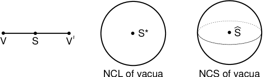
Figure 1: Configuration space: vacua and sphalerons.

The nonperturbative $Sp(n)$ (Witten) anomaly [6] is also related to a sphaleron, namely the solution $\mathrm{S}^{\star}$ constructed in Ref. [18]. The electroweak sphaleron $\mathrm{S}^{\star}$ sets the energy barrier for the Witten anomaly (which cancels out in the Standard Model) and may play a role for the asymptotics of perturbation theory [19] and in multiparticle dynamics [20].

An example of an anomalous and inconsistent theory is the chiral $Sp(2)=SU(2)$ gauge theory with a single doublet of left-handed Weyl fermions. In this case, there is a noncontractible loop (NCL) of gauge field vacua (corresponding to the nontrivial element of $\pi_{4}[SU(2)]$) at the edge of a two-dimensional disc in configuration space. For one “point” of the disc ($\mathrm{S}^{\star}$ in the Yang–Mills–Higgs theory), there are crossing fermionic levels. The sphaleron $\mathrm{S}^{\star}$ has indeed two fermion zero modes [20, 21]. The Witten anomaly results from the Berry phase factor $-1$ for a single closed path around these degenerate fermionic levels [22]. This phase factor gives a Möbius bundle structure over the edge of the disc (the NCL of gauge field vacua), which prevents the continuous implementation of Gauss’ law. In other words, the nontrivial Berry phase factor presents an insurmountable obstruction to the implementation of Gauss’ law and physical states are no longer gauge invariant [6, 8]. A two-dimensional slice of $SU(2)$ Yang–Mills–Higgs configuration space is sketched in the middle part of Fig. 1.

There remains the perturbative non-Abelian (Bardeen) anomaly [3, 4, 7]. An example of an anomalous and inconsistent theory is the chiral $SU(3)$ gauge theory with a single triplet of left-handed Weyl fermions. Now, there is a noncontractible sphere (NCS) of gauge field vacua (corresponding to the generator of $\pi_{5}[SU(3)]$) at the border of a three–ball in configuration space. By the family index theorem, there are crossing energy levels of the Dirac Hamiltonian at one “point” of the three–ball [8]. The non-Abelian anomaly is the Berry phase [22] from these degenerate fermionic levels.

Again, a nonzero Berry phase ($\mathrm{mod}\>2\pi$) presents an obstruction to the implementation of Gauss’ law. The Berry phase of a loop on the NCS considered does not vanish and is, in fact, equal to one half of the solid angle subtended at the “point” with crossing energy levels by the loop; see Refs. [8, 22] for further details and Fig. 2 for a sketch. It has been conjectured [23] that this special “point” in configuration space corresponds to a new type of sphaleron in $SU(3)$ Yang–Mills–Higgs theory (denoted by $\widehat{\mathrm{S}}$ in the right part of Fig. 1) and the goal of the present article is to establish the basic properties of this sphaleron.

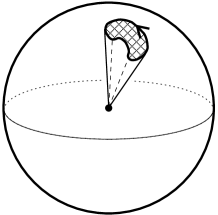
Figure 2: $SU(3)$ Bardeen anomaly as Berry phase.

The outline of our article is as follows. Section 2 recalls the action of chiral $SU(3)$ gauge theory, mainly in order to establish notation. Section 3 discusses the topology responsible for the new sphaleron, together with approximate bosonic field configurations. Section 4 presents the generalized Ansatz for the bosonic fields, which can be shown to solve the field equations consistently. Section 5 gives the corresponding Ansatz for the fermionic field, together with analytic and numerical results which suggest the existence of two fermion zero modes. Section 6 presents some concluding remarks. Three appendices give the Ansatz energy density for the bosonic fields, an argument in favor of a nontrivial regular solution of the reduced field equations, and the fermion zero modes for a related gauge field background.

2 Chiral $SU(3)$ gauge theory

In this article, we consider a relatively simple theory, namely $SU(3)$ Yang–Mills–Higgs theory with a single triplet of complex scalar fields and a single triplet of massless left-handed Weyl fermions, both in the complex $\mathbf{3}$ representation of $SU(3)$. Our results can be readily extended to other gauge groups $G$ with $\pi_{5}[G]=\Zset$ and appropriate representations.

The chiral $SU(3)$ gauge theory has the following classical action:

$$S=\int_{\mathbb{R}^{4}}\;\!{\rm d}^{4}x\,\,\left\{{\textstyle\frac{1}{2}}\,\text{tr}\,F_{\mu\nu}F^{\mu\nu}+(D_{\mu}\Phi)^{\dagger}\,(D^{\mu}\Phi)-\lambda\,\left(\Phi^{\dagger}\Phi-\eta^{2}\right)^{2}+{\rm i}\,\bar{\psi}\,\sigma^{\mu}D_{\mu}\,\psi\right\}\,,$$ (2.1)

where $F_{\mu\nu}\equiv\partial_{\mu}A_{\nu}-\partial_{\nu}A_{\mu}+g[A_{\mu},A_{\nu}]$ is the $SU(3)$ Yang–Mills field strength tensor and $D_{\mu}\equiv(\partial_{\mu}+gA_{\mu})$ the covariant derivative for the $\mathbf{3}$ representation.

The $SU(3)$ Yang–Mills gauge field is defined as

$$A_{\mu}(x)\equiv A_{\mu}^{a}(x)\,\lambda_{a}/(2{\rm i})\,,$$ (2.2)

in terms of the eight Gell-Mann matrices

$$\lambda_{1} =\left(\begin{array}[]{c@{\hspace{4mm}}c@{\hspace{4mm}}c}0\hfil\hskip 11.38109pt&1\hfil\hskip 11.38109pt&0\\[-4.30554pt] 1\hfil\hskip 11.38109pt&0\hfil\hskip 11.38109pt&0\\[-4.30554pt] 0\hfil\hskip 11.38109pt&0\hfil\hskip 11.38109pt&0\end{array}\right)\,, \lambda_{2} =\left(\begin{array}[]{c@{\hspace{4mm}}c@{\hspace{4mm}}c}0\hfil\hskip 11.38109pt&-{\rm i}\hfil\hskip 11.38109pt&0\\[-4.30554pt] {\rm i}\hfil\hskip 11.38109pt&0\hfil\hskip 11.38109pt&0\\[-4.30554pt] 0\hfil\hskip 11.38109pt&0\hfil\hskip 11.38109pt&0\end{array}\right)\,, \lambda_{3} =\left(\begin{array}[]{c@{\hspace{4mm}}c@{\hspace{4mm}}c}1\hfil\hskip 11.38109pt&0\hfil\hskip 11.38109pt&0\\[-4.30554pt] 0\hfil\hskip 11.38109pt&-1\hfil\hskip 11.38109pt&0\\[-4.30554pt] 0\hfil\hskip 11.38109pt&0\hfil\hskip 11.38109pt&0\end{array}\right)\,,$$ (2.12)

$$\lambda_{4} =\left(\begin{array}[]{c@{\hspace{4mm}}c@{\hspace{4mm}}c}0\hfil\hskip 11.38109pt&0\hfil\hskip 11.38109pt&1\\[-4.30554pt] 0\hfil\hskip 11.38109pt&0\hfil\hskip 11.38109pt&0\\[-4.30554pt] 1\hfil\hskip 11.38109pt&0\hfil\hskip 11.38109pt&0\end{array}\right)\,, \lambda_{5} =\left(\begin{array}[]{c@{\hspace{4mm}}c@{\hspace{4mm}}c}0\hfil\hskip 11.38109pt&0\hfil\hskip 11.38109pt&-{\rm i}\\[-4.30554pt] 0\hfil\hskip 11.38109pt&0\hfil\hskip 11.38109pt&0\\[-4.30554pt] {\rm i}\hfil\hskip 11.38109pt&0\hfil\hskip 11.38109pt&0\end{array}\right)\,, \lambda_{6} =\left(\begin{array}[]{c@{\hspace{4mm}}c@{\hspace{4mm}}c}0\hfil\hskip 11.38109pt&0\hfil\hskip 11.38109pt&0\\[-4.30554pt] 0\hfil\hskip 11.38109pt&0\hfil\hskip 11.38109pt&1\\[-4.30554pt] 0\hfil\hskip 11.38109pt&1\hfil\hskip 11.38109pt&0\end{array}\right)\,,$$ (2.22)

$$\lambda_{7} =\left(\begin{array}[]{c@{\hspace{4mm}}c@{\hspace{4mm}}c}0\hfil\hskip 11.38109pt&0\hfil\hskip 11.38109pt&0\\[-4.30554pt] 0\hfil\hskip 11.38109pt&0\hfil\hskip 11.38109pt&-{\rm i}\\[-4.30554pt] 0\hfil\hskip 11.38109pt&{\rm i}\hfil\hskip 11.38109pt&0\end{array}\right)\,, \lambda_{8} =\frac{1}{\sqrt{3}}\left(\begin{array}[]{c@{\hspace{4mm}}c@{\hspace{4mm}}c}1\hfil\hskip 11.38109pt&0\hfil\hskip 11.38109pt&0\\[-4.30554pt] 0\hfil\hskip 11.38109pt&1\hfil\hskip 11.38109pt&0\\[-4.30554pt] 0\hfil\hskip 11.38109pt&0\hfil\hskip 11.38109pt&-2\end{array}\right)\,.$$ (2.29)

The field $\Phi(x)$ is a triplet of complex scalar fields, which acquires a vacuum expectation value $\eta$ due to the Higgs potential term in the action (2.1). The field $\psi(x)$ is a triplet of two-component Weyl spinors and $\bar{\psi}(x)$ its complex conjugate. Also, we define $(\sigma^{\mu})\equiv(\mathbf{1},-\vec{\sigma})$ in terms of the Pauli matrices $\vec{\sigma}$ and use the Minkowski space metric with $g_{\mu\nu}(x)={\rm diag}(+1,-1,-1,-1)$ and natural units with $\hbar=c=1$.

For static three-dimensional field configurations, we generally employ the spherical polar coordinates $(r,\theta,\phi)$ but sometimes also the cylindrical coordinates $(\rho,\phi,z)$, with $\rho\equiv r\,\sin\theta$ and $z\equiv r\,\cos\theta$.

3 Topology and approximate sphaleron

The basic motivation for our search of a new sphaleron ($\widehat{\mathrm{S}}$) in $SU(3)$ Yang–Mills–Higgs theory has been given in the penultimate paragraph of Section 1 and was summarized by Fig. 2. We start with the bosonic fields of the theory (2.1) and introduce a topologically nontrivial map $S^{3}\wedge S^{2}\to SU(3)$, with parameters $(\psi,\mu,\alpha)$ and coordinates $(\theta,\phi)$ on the “sphere at infinity.” Here, $\wedge$ denotes the so-called smash product which topologically transforms the Cartesian product $S^{p}\times S^{m}$ to $S^{p+m}$ by contracting, for fixed points $x_{0}\in S^{p}$ and $y_{0}\in S^{m}$, the set $\{x_{0}\}\times S^{m}\cup S^{p}\times\{y_{0}\}$ to a single point. Topologically, one has therefore $S^{p}\wedge S^{m}\sim S^{p+m}$; cf. Ref. [21].

The procedure to be followed is similar to the one used for the sphalerons S [10, 11] and $\mathrm{S}^{\star}$ [18], which employed maps $S^{1}\wedge S^{2}\to SU(2)$ and $S^{2}\wedge S^{2}\to SU(2)$, respectively. The reason behind this particular choice of smash products is that the search of new solutions is best performed in a fixed gauge, which we take to be the radial gauge (hence, $\theta$ and $\phi$ appear in the maps, but not $r$). The three–ball of Fig. 2 or the right part of Fig. 1 becomes in the radial gauge a three–sphere (parametrized by $\psi$, $\mu$, and $\alpha$) with $\widehat{\mathrm{S}}$ at the top and $\mathrm{V}$ at the bottom, where the “height” corresponds to the energy of the configuration. See, e.g., Refs. [10, 21] for further details.

The following “strikingly simple” map [24] is a generator of $\pi_{5}[SU(3)]=\mathbb{Z}$:

$$U:S^{5}\to SU(3)\,,\quad U(z_{1},z_{2},z_{3})=\left(\begin{array}[]{ccc}z_{1}^{2}&\;\;z_{1}\,z_{2}-\bar{z}_{3}&\;\;z_{1}\,z_{3}+\bar{z}_{2}\\ z_{1}\,z_{2}+\bar{z}_{3}&\;\;z_{2}^{2}&\;\;z_{2}\,z_{3}-\bar{z}_{1}\\ z_{1}\,z_{3}-\bar{z}_{2}&\;\;z_{2}\,z_{3}+\bar{z}_{1}&\;\;z_{3}^{2}\end{array}\right)\,,$$ (3.1)

with $z_{1},z_{2},z_{3}\in\mathbb{C}$ and $|z_{1}|^{2}+|z_{2}|^{2}+|z_{3}|^{2}=1$. An appropriate parametrization for our purpose is

$$\left(\begin{array}[]{c}z_{1}\\[4.30554pt] z_{2}\\[4.30554pt] z_{3}\end{array}\right)\equiv\left(\begin{array}[]{c}1-\cos^{2}\frac{\theta}{2}\,(1-\cos\psi)+{\rm i}\,\cos\frac{\theta}{2}\sin\psi\cos\mu\\[4.30554pt] {\rm e}^{{\rm i}\phi}\,\sin\frac{\theta}{2}\,\cos\frac{\theta}{2}\,(1-\cos\psi)\\[4.30554pt] \cos\frac{\theta}{2}\,\sin\psi\,\sin\mu\,(\sin\alpha+{\rm i}\,\cos\alpha)\end{array}\right)\,,$$ (3.2)

with angles $\psi,\mu,\theta\in[0,\pi]$ and $\alpha,\phi\in[0,2\pi]$. At first sight, Eq. (3.2) constitutes a map $S^{3}\times S^{2}\to S^{5}$, with $S^{3}$ parametrized by spherical polar coordinates $(\psi,\mu,\alpha)$ and $S^{2}$ by $(\theta,\phi)$. But the expression on the right-hand side of Eq. (3.2) corresponds to the single point $(z_{1},z_{2},z_{3})=(1,0,0)$ if either $\psi=0$ or $\theta=\pi$ and the map (3.2) is effectively $S^{3}\wedge S^{2}\to S^{5}$. The fixed points $x_{0}\in S^{3}$ and $y_{0}\in S^{2}$ needed for the smash product are thus given by $\psi=0$ and $\theta=\pi$, respectively.

For $\psi=0$, the matrix $U(z_{1},z_{2},z_{3})$ is independent of the parameters $\mu$ and $\alpha$ and the coordinates $\theta$ and $\phi$,

$$V\equiv U(\psi,\mu,\alpha,\theta,\phi)\bigr{|}_{\,\psi=0}=\left(\begin{array}[]{c@{\hspace{4mm}}c@{\hspace{4mm}}c}1\hfil\hskip 11.38109pt&0\hfil\hskip 11.38109pt&0\\[-4.30554pt] 0\hfil\hskip 11.38109pt&0\hfil\hskip 11.38109pt&-1\\[-4.30554pt] 0\hfil\hskip 11.38109pt&+1\hfil\hskip 11.38109pt&0\end{array}\right)\,.$$ (3.3)

For $\psi=\pi$, the matrix $U(z_{1},z_{2},z_{3})$ is independent of $\mu$ and $\alpha$ but does depend on $\theta$ and $\phi$,

$$W(\theta,\phi) \equiv U(\psi,\mu,\alpha,\theta,\phi)\bigr{|}_{\,\psi=\pi}$$

$$=\left(\begin{array}[]{ccc}\cos^{2}\theta&\;\;-\cos\theta\,\sin\theta\,{\rm e}^{{\rm i}\phi}&\;\;\sin\theta\,{\rm e}^{-{\rm i}\phi}\\[4.30554pt] -\cos\theta\,\sin\theta\,{\rm e}^{{\rm i}\phi}&\;\;\sin^{2}\theta\,{\rm e}^{2{\rm i}\phi}&\;\;\cos\theta\\[4.30554pt] -\sin\theta\,{\rm e}^{-{\rm i}\phi}&\;\;-\cos\theta&\;\;0\end{array}\right)\,.$$ (3.7)

These two matrices have the following rotation and reflection symmetries:

$$\partial_{\phi}\,M+\frac{{\rm i}}{2}\,\left(\lambda_{3}-\sqrt{3}\,\lambda_{8}\right)M+\frac{{\rm i}}{2}\,M\left(\lambda_{3}-\sqrt{3}\,\lambda_{8}\right)=0\,,$$ (3.8a)

$$V(\theta,\phi)=V(\pi-\theta,\phi)\,,$$ (3.8b)

$$\left(\begin{array}[]{c@{\hspace{4mm}}c@{\hspace{4mm}}c}-1\hfil\hskip 11.38109pt&0\hfil\hskip 11.38109pt&0\\[-4.30554pt] 0\hfil\hskip 11.38109pt&1\hfil\hskip 11.38109pt&0\\[-4.30554pt] 0\hfil\hskip 11.38109pt&0\hfil\hskip 11.38109pt&-1\end{array}\right)\,W(\theta,\phi)\,\left(\begin{array}[]{c@{\hspace{4mm}}c@{\hspace{4mm}}c}-1\hfil\hskip 11.38109pt&0\hfil\hskip 11.38109pt&0\\[-4.30554pt] 0\hfil\hskip 11.38109pt&1\hfil\hskip 11.38109pt&0\\[-4.30554pt] 0\hfil\hskip 11.38109pt&0\hfil\hskip 11.38109pt&-1\end{array}\right)=W(\pi-\theta,\phi)\,,$$ (3.8i)

for $M=V$ and $W$ as defined by Eqs. (3.3) and (3.7), with a trivial $(\theta,\phi)$ dependence for $V$.

Observe that the general matrix $U(\psi,\mu,\alpha,\theta,\phi)$ possesses the reflection symmetries (3.8bc) only for $\psi=0$ and $\pi$. The “point” $\psi=0$ with $U=V$ and its “antipode” $\psi=\pi$ with $U=W$ will be shown to correspond to the (unique) vacuum solution $\mathrm{V}$ and the new sphaleron $\widehat{\mathrm{S}}$, respectively. As mentioned above, there is, in the radial gauge, a three–sphere with $\widehat{\mathrm{S}}$ at the top ($\psi=\pi$) and $\mathrm{V}$ at the bottom ($\psi=0$), where the “height” corresponds to the energy of the configuration.

The Cartesian components of the sphaleron-like $SU(3)$ gauge field configuration are now defined as follows:

$$A_{0}(r,\theta,\phi)=0\,,\quad A_{m}(r,\theta,\phi)=-g^{-1}\,f(r)\,\partial_{m}W(\theta,\phi)\>W^{-1}(\theta,\phi)\,,$$ (3.9)

with $m=1,2,3$, and the following boundary conditions on the radial function:

$$f(0)=0\,,\quad\lim_{r\to\infty}f(r)=1\,.$$ (3.10)

The corresponding Higgs field configuration is given by

$$\Phi(r,\theta,\phi)=h(r)\,\eta\,W(\theta,\phi)\,\left(\begin{array}[]{c}1\\ 0\\ 0\end{array}\right)\,,$$ (3.11)

with the following boundary conditions:

$$h(0)=0\,,\quad\lim_{r\to\infty}h(r)=1\,.$$ (3.12)

More specifically, the radial functions $f(r)$ and $h(r)$ are even and odd in $r$, with $f(r)\propto r^{2}$ and $h(r)\propto r$ near the origin.

For the vacuum solution $\mathrm{V}$, the matrix $W(\theta,\phi)$ in Eqs. (3.9) and (3.11) is replaced by the constant matrix $V$ defined by Eq. (3.3) and the profile function $h(r)$ in Eq. (3.11) by the constant value $1$. The vacuum field configurations are then $A_{0}=A_{m}=0$ and $\Phi=\eta\,(1,0,0)^{\mathrm{\,t}}$, with $\mathrm{t}$ standing for the transpose.

The gauge and Higgs fields of Eqs. (3.9) and (3.11) are static and in the radial gauge ($A_{r}=0$). They carry the basic structure of the sphaleron $\widehat{\mathrm{S}}$ but are not general enough to solve the field equations consistently. In the next section, we present a suitable generalization.

4 Sphaleron Ansatz

4.1 Bosonic fields

As shown in the previous section, the matrix function $W(\theta,\phi)$ from Eq. (3.7) has an axial symmetry given by Eq. (3.8a). This implies that the gauge field (3.9), with spherical components defined by

$$A_{\phi} \equiv-g^{-1}\,f(r)\,\partial_{\phi}W\,W^{-1}\,, A_{\theta} \equiv-g^{-1}\,f(r)\,\partial_{\theta}W\,W^{-1}\,, A_{r} \equiv 0\,,$$ (4.1)

has the property

$$\partial_{\phi}A_{c}=[-2\,U_{3},A_{c}]\,,$$ (4.2)

where $c$ stands for the component $\phi$, $\theta$, or $r$, and $2\,U_{3}$ is a constant matrix,

$$-2\,U_{3}\equiv-\frac{{\rm i}}{2}(\lambda_{3}-\sqrt{3}\,\lambda_{8})={\rm i}\left(\begin{array}[]{c@{\hspace{4mm}}c@{\hspace{4mm}}c}0\hfil\hskip 11.38109pt&0\hfil\hskip 11.38109pt&0\\[-4.30554pt] 0\hfil\hskip 11.38109pt&1\hfil\hskip 11.38109pt&0\\[-4.30554pt] 0\hfil\hskip 11.38109pt&0\hfil\hskip 11.38109pt&-1\end{array}\right)\,.$$ (4.3)

Next, introduce the following sets of matrices:

$$T_{\phi} \equiv-\sin\phi\,\frac{\lambda_{1}}{2{\rm i}}+\cos\phi\,\frac{\lambda_{2}}{2{\rm i}}\,, T_{\rho} \equiv\cos\phi\,\frac{\lambda_{1}}{2{\rm i}}+\sin\phi\,\frac{\lambda_{2}}{2{\rm i}}\,,$$

$$T_{3} \equiv\frac{\lambda_{3}}{2{\rm i}}\,,$$ (4.4a)

$$V_{\phi} \equiv+\sin\phi\,\frac{\lambda_{4}}{2{\rm i}}+\cos\phi\,\frac{\lambda_{5}}{2{\rm i}}\,, V_{\rho} \equiv\cos\phi\,\frac{\lambda_{4}}{2{\rm i}}-\sin\phi\,\frac{\lambda_{5}}{2{\rm i}}\,,$$

$$V_{3} \equiv\frac{\sqrt{3}\,\lambda_{8}+\lambda_{3}}{4{\rm i}}\,,$$ (4.4b)

$$U_{\phi} \equiv\sin(2\phi)\,\frac{\lambda_{6}}{2{\rm i}}+\cos(2\phi)\,\frac{\lambda_{7}}{2{\rm i}}\,, U_{\rho} \equiv\cos(2\phi)\,\frac{\lambda_{6}}{2{\rm i}}-\sin(2\phi)\,\frac{\lambda_{7}}{2{\rm i}}\,,$$

$$U_{3} \equiv\frac{\sqrt{3}\,\lambda_{8}-\lambda_{3}}{4{\rm i}}\,,$$ (4.4c)

which have the same property

$$\partial_{\phi}X=[-2U_{3},X]\,,$$ (4.5)

with $X$ standing for any of the matrices defined in Eqs. (4.4abc). The sets $\{T_{a}\}$, $\{V_{a}\}$, $\{U_{a}\}$ generate the three $su(2)$ subalgebras of $su(3)$ known as $T$–spin, $V$–spin, and $U$–spin. Since $T_{3}$, $V_{3}$, and $U_{3}$ are not independent, we will use the basis $\{T_{\phi}$, $T_{\rho}$, $V_{\phi}$, $V_{\rho}$, $U_{\phi}$, $U_{\rho}$, $\lambda_{3}/(2{\rm i})$, $\lambda_{8}/(2{\rm i})\}$ of $su(3)$ in the subsequent discussion.

The gauge field (3.9) of the approximate sphaleron can be expanded in terms of this $su(3)$ basis. It turns out that the component $A_{\phi}$ involves only $T_{\rho}$, $V_{\rho}$, $U_{\rho}$, $\lambda_{3}/(2{\rm i})$, $\lambda_{8}/(2{\rm i})$, and that $A_{\theta}$ involves only $T_{\phi}$, $V_{\phi}$, $U_{\phi}$. An Ansatz which has this structure and which generalizes (3.9) is given by

$$g\,\widehat{A}_{0}(r,\theta,\phi) = 0\,,$$ (4.6a)

$$g\,\widehat{A}_{\phi}(r,\theta,\phi) = \alpha_{1}(r,\theta)\,\cos\theta\;T_{\rho}+\alpha_{2}(r,\theta)\;V_{\rho}+\alpha_{3}(r,\theta)\,\cos\theta\;U_{\rho}+$$ (4.6b)

$$\alpha_{4}(r,\theta)\;\frac{\lambda_{3}}{2{\rm i}}+\alpha_{5}(r,\theta)\;\frac{\lambda_{8}}{2{\rm i}}\,,$$

$$g\,\widehat{A}_{\theta}(r,\theta,\phi) = \alpha_{6}(r,\theta)\;T_{\phi}+\alpha_{7}(r,\theta)\,\cos\theta\;V_{\phi}+\alpha_{8}(r,\theta)\;U_{\phi}\,,$$ (4.6c)

$$g\,\widehat{A}_{r}(r,\theta,\phi) = \frac{1}{r}\>\Bigl{[}\,\alpha_{9}(r,\theta)\,\cos\theta\;T_{\phi}+\alpha_{10}(r,\theta)\;V_{\phi}+\alpha_{11}(r,\theta)\,\cos\theta\;U_{\phi}\Bigr{]}\,,$$ (4.6d)

with real functions $\alpha_{j}$, for $j=1,\ldots,11$, depending on $r$ and $\theta$ and matrices $T,V,U$ from Eqs. (4.4abc) depending implicitly on $\phi$. There are the following boundary conditions at the coordinate origin ($r=0$):

$$\alpha_{j}(0,\theta)=0\,,\quad\mathrm{for}\;\;j=1,\ldots,11,$$ (4.7)

on the symmetry axis ($\bar{\theta}=0,\pi$):

$$\alpha_{j}(r,\bar{\theta}) =\bar{\alpha}_{j}(r)\,\sin\theta\,\bigr{|}_{\,\theta=\bar{\theta}}\,, \mathrm{for}\;\;j =1,2,9,10,$$ (4.8a)

$$\alpha_{j}(r,\bar{\theta}) =\bar{\alpha}_{j}(r)\,\sin^{2}\theta\,\bigr{|}_{\,\theta=\bar{\theta}}\,, \mathrm{for}\;\;j =3,4,5,11,$$ (4.8b)

$$\alpha_{j}(r,\bar{\theta}) =(-)^{j-5}\,\cos\theta\,\partial_{\theta}\,\alpha_{j-5}(r,\theta)\,\bigr{|}_{\,\theta=\bar{\theta}}\,, \mathrm{for}\;\;j =6,7,$$ (4.8c)

$$\alpha_{j}(r,\bar{\theta}) ={\textstyle\frac{1}{2}}\,\cos\theta\,\partial_{\theta}\,\alpha_{j-5}(r,\theta)\,\bigr{|}_{\,\theta=\bar{\theta}}\,, \mathrm{for}\;\;j =8,$$ (4.8d)

and towards infinity:

$$\lim_{r\to\infty}\,\left(\begin{array}[]{c}\alpha_{1}(r,\theta)\\ \alpha_{2}(r,\theta)\\ \alpha_{3}(r,\theta)\\ \alpha_{4}(r,\theta)\\ \alpha_{5}(r,\theta)\\ \alpha_{6}(r,\theta)\\ \alpha_{7}(r,\theta)\\ \alpha_{8}(r,\theta)\\ \alpha_{9}(r,\theta)\\ \alpha_{10}(r,\theta)\\ \alpha_{11}(r,\theta)\end{array}\right)=\left(\begin{array}[]{c}-2\,\sin\theta\,(1+\sin^{2}\theta)\\ 2\,\sin\theta\,\cos^{2}\theta\\ -2\sin^{2}\theta\\ -\sin^{2}\theta\,(1+2\,\sin^{2}\theta)\\ \sqrt{3}\,\sin^{2}\theta\\ 2\\ 2\\ -2\,\sin\theta\\ 0\\ 0\\ 0\end{array}\right)\,.$$ (4.9)

Furthermore, the $\alpha_{j}$ are required to have positive parity with respect to reflection of the $z$-coordinate,

$$\alpha_{j}(r,\pi-\theta)=+\alpha_{j}(r,\theta)\,,\quad\mathrm{for}\;\;j=1,\ldots,11,$$ (4.10)

in order to keep the reflection symmetry of the approximate sphaleron configuration; cf. Eqs. (3.8i) and (3.9). For completeness, the Cartesian components of the gauge field Ansatz are

$$g\,\widehat{A}_{1}= -\,\frac{\sin\phi}{\rho}\Bigl{[}\,\alpha_{1}\cos\theta\,T_{\rho}+\alpha_{2}V_{\rho}+\alpha_{3}\cos\theta\,U_{\rho}+\alpha_{4}\lambda_{3}/(2{\rm i})+\alpha_{5}\lambda_{8}/(2{\rm i})\,\Bigr{]}$$

$$+\,\frac{\sin\theta\,\cos\phi}{\rho}\Bigl{[}\,\cos\theta(\alpha_{6}+\sin\theta\,\alpha_{9})\,T_{\phi}+(\cos^{2}\theta\,\alpha_{7}+\sin\theta\,\alpha_{10})\,V_{\phi}$$

$$+\,\cos\theta(\alpha_{8}+\sin\theta\,\alpha_{11})\,U_{\phi}\,\Bigr{]}\,,$$ (4.11a)

$$g\,\widehat{A}_{2}= \frac{\cos\phi}{\rho}\Bigl{[}\,\alpha_{1}\cos\theta\,T_{\rho}+\alpha_{2}V_{\rho}+\alpha_{3}\cos\theta\,U_{\rho}+\alpha_{4}\lambda_{3}/(2{\rm i})+\alpha_{5}\lambda_{8}/(2{\rm i})\,\Bigr{]}$$

$$+\,\frac{\sin\theta\,\sin\phi}{\rho}\Bigl{[}\,\cos\theta\,(\alpha_{6}+\sin\theta\,\alpha_{9})\,T_{\phi}+(\cos^{2}\theta\,\alpha_{7}+\sin\theta\,\alpha_{10})\,V_{\phi}$$

$$+\,\cos\theta(\alpha_{8}+\sin\theta\,\alpha_{11})\,U_{\phi}\,\Bigr{]}\,,$$ (4.11b)

$$g\,\widehat{A}_{3}= -\,\frac{\cos\theta}{z}\Bigl{[}\,(\sin\theta\,\alpha_{6}-\cos^{2}\theta\,\alpha_{9})\,T_{\phi}+\cos\theta\,(\sin\theta\,\alpha_{7}-\alpha_{10})\,V_{\phi}$$

$$+\,(\sin\theta\,\alpha_{8}-\cos^{2}\theta\,\alpha_{11})\,U_{\phi}\,\Bigr{]}\,,$$ (4.11c)

with a $T$–spin structure similar to the $\mathrm{S}$ and $\mathrm{S}^{\star}$ Ansätze [18].

Turning to the Higgs field (3.11) of the approximate sphaleron, we observe that the direction of the vacuum expectation value has been chosen so that $2\,U_{3}\Phi_{\rm vac}=0$. The field $\Phi$ is found to have an axial symmetry,

$$\partial_{\phi}\Phi=-2\,U_{3}\,\Phi\,,$$ (4.12)

which matches the axial symmetry (4.2) of the gauge field. The structure of this specific Higgs field is now generalized to the following Ansatz:

$$\widehat{\Phi}(r,\theta,\phi) = \eta\,\bigl{[}\,\beta_{1}(r,\theta)\,\lambda_{3}+\beta_{2}(r,\theta)\,\cos\theta\;\,2{\rm i}\,T_{\rho}+\beta_{3}(r,\theta)\,2{\rm i}\,V_{\rho}\,\bigr{]}\,\left(\begin{array}[]{c}1\\ 0\\ 0\end{array}\right)$$ (4.16)

$$= \eta\,\left(\begin{array}[]{l}\beta_{1}(r,\theta)\\ \beta_{2}(r,\theta)\,\cos\theta\;{\rm e}^{{\rm i}\phi}\\ \beta_{3}(r,\theta)\;{\rm e}^{-{\rm i}\phi}\end{array}\right)\,,$$ (4.20)

with real functions $\beta_{k}$, for $k=1,2,3$, depending on $r$ and $\theta$ and matrices $T_{\rho}$ and $V_{\rho}$ depending implicitly on $\phi$. The boundary conditions are at the coordinate origin ($r=0$):

$$\partial_{\theta}\,\beta_{1}(0,\theta)=\beta_{2}(0,\theta)=\beta_{3}(0,\theta)=0\,,$$ (4.21)

on the symmetry axis ($\bar{\theta}=0,\pi$):

$$\partial_{\theta}\,\beta_{1}(r,\theta)\,\bigr{|}_{\,\theta=\bar{\theta}}=0\,,\quad\beta_{k}(r,\bar{\theta})=\bar{\beta}_{k}(r)\,\sin\theta\,\bigr{|}_{\,\theta=\bar{\theta}}\,,\quad\mathrm{for}\;\;k=2,3,$$ (4.22)

and towards infinity:

$$\lim_{r\to\infty}\,\left(\begin{array}[]{c}\beta_{1}(r,\theta)\\ \beta_{2}(r,\theta)\\ \beta_{3}(r,\theta)\end{array}\right)=\left(\begin{array}[]{c}\cos^{2}\theta\\ -\sin\theta\\ -\sin\theta\end{array}\right)\,.$$ (4.29)

Furthermore, these functions must be even under reflection of the $z$-coordinate,

$$\beta_{k}(r,\pi-\theta) =+\beta_{k}(r,\theta)\,,\quad\mathrm{for}\;\;k=1,2,3.$$ (4.30)

This completes the construction of the Ansatz for the bosonic fields. Before discussing the resulting energy and field equations, the following three remarks may be helpful. First, the gauge field (3.9) and Higgs field (3.11) of the approximate sphaleron are reproduced by the following Ansatz functions:

$$\left(\begin{array}[]{c}\alpha_{1}(r,\theta)\\ \alpha_{2}(r,\theta)\\ \alpha_{3}(r,\theta)\\ \alpha_{4}(r,\theta)\\ \alpha_{5}(r,\theta)\\ \alpha_{6}(r,\theta)\\ \alpha_{7}(r,\theta)\\ \alpha_{8}(r,\theta)\\ \alpha_{9}(r,\theta)\\ \alpha_{10}(r,\theta)\\ \alpha_{11}(r,\theta)\end{array}\right) = \,f(r)\,\left(\begin{array}[]{c}-2\,\sin\theta\,(1+\sin^{2}\theta)\\ 2\,\sin\theta\,\cos^{2}\theta\\ -2\sin^{2}\theta\\ -\sin^{2}\theta\,(1+2\,\sin^{2}\theta)\\ \sqrt{3}\,\sin^{2}\theta\\ 2\\ 2\\ -2\,\sin\theta\\ 0\\ 0\\ 0\end{array}\right)\,,$$ (4.31w)

$$\left(\begin{array}[]{c}\beta_{1}(r,\theta)\\ \beta_{2}(r,\theta)\\ \beta_{3}(r,\theta)\end{array}\right) = \,h(r)\,\left(\begin{array}[]{c}\cos^{2}\theta\\ -\sin\theta\\ -\sin\theta\end{array}\right)\,,$$ (4.31ad)

which explains in part the choice of boundary conditions (4.7)–(4.9) and (4.21)–(4.29) for the general Ansatz.

Second, the Ansatz as given by Eqs. (4.6) and (4.20) has a residual $SO(3)$ gauge symmetry under the following transformations:

$$g\,\widehat{A}^{\prime}_{n}=\Omega\,\left(\,g\,\widehat{A}_{n}+\partial_{n}\,\right)\,\Omega^{-1}\,,\quad\widehat{\Phi}^{\prime}=\Omega\,\widehat{\Phi}\,,$$ (4.32a)

with

$$\Omega(r,\theta,\phi)\equiv\exp\bigl{[}\,\omega_{T}(r,\theta)\,T_{\phi}+\omega_{V}(r,\theta)\,V_{\phi}+\omega_{U}(r,\theta)\,U_{\phi}\,\bigr{]}\,,$$ (4.32b)

for two-dimensional parameter functions $\omega_{s}(r,\theta)$, $s=T,V,U$.

Third, the structure of the Ansatz gauge field (4.6) is quite intricate: for a given halfplane through the $z$–axis with azimuthal angle $\phi$, the parallel components $\widehat{A}_{r}$ and $\widehat{A}_{\theta}$ involve only one particular $su(2)$ subalgebra of $su(3)$, whereas the orthogonal component $\widehat{A}_{\phi}$ excites precisely the other five generators of $su(3)$.

4.2 Energy and field equations

The bosonic energy functional of theory (2.1) is given by

$$E[A,\Phi]=\int_{\mathbb{R}^{3}}\!{\rm d}^{3}x\,\,\left[\,-{\textstyle\frac{1}{2}}\,{\rm tr}(F_{mn})^{2}+|D_{m}\Phi|^{2}+\lambda\left(|\Phi|^{2}-\eta^{2}\right)^{2}\,\right]\,,$$ (4.33)

for spatial indices $m,n=1,2,3$. From the sphaleron Ansätze (4.6) and (4.20), one obtains

$$E[\widehat{A},\widehat{\Phi}]=4\pi\int_{0}^{\infty}\!{\rm d}r\,\,\int_{0}^{\pi/2}\!{\rm d}\theta\,\,\,r^{2}\sin\theta\;\,\widehat{e}(r,\theta)\,,$$ (4.34)

where the energy density $\widehat{e}(r,\theta)$ contains contributions from the Yang–Mills term, the kinetic Higgs term, and the Higgs potential in the energy functional,

$$\widehat{e}(r,\theta) =\widehat{e}_{\rm\,YM}(r,\theta)+\widehat{e}_{\rm\,Hkin}(r,\theta)+\widehat{e}_{\rm\,Hpot}(r,\theta)\,.$$ (4.35)

The detailed expressions for these energy density contributions are relegated to Appendix A. The energy density (4.35) turns out to be well-behaved due to the boundary conditions (4.7)–(4.9) and (4.21)–(4.29). In addition, there is a reflection symmetry, $\widehat{e}(r,\theta)=\widehat{e}(r,\pi-\theta)$, which allows the range of $\theta$ in Eq. (4.34) to be restricted to $[0,\pi/2]$.

It can be verified that the Ansätze (4.6)–(4.10) and (4.20)–(4.30) consistently solve the field equations of the theory (2). That is, they reproduce the variational equations from the Ansatz energy functional (4.34). This result is a manifestation of the principle of symmetric criticality [25], which states that in the quest of stationary points it suffices, under certain conditions, to consider variations that respect the symmetries of the Ansatz (here, rotation and reflection symmetries).

It is difficult to prove that the resulting system of partial differential equations for the Ansatz functions $\alpha_{j}(r,\theta)$ and $\beta_{k}(r,\theta)$, together with the conditions (4.7)–(4.10) and (4.21)–(4.30), has a nontrivial solution, that is, a non-vacuum solution. It is, however, possible to give a heuristic argument in favor of a nontrivial regular solution (a similar argument has been used for $\mathrm{S}^{\star}$ [18]).

According to the boundary condition (4.29), the function $\beta_{1}(r,\theta)$ vanishes asymptotically for $\theta=\pi/2$, i.e., on the equatorial circle at infinity. Let us simply exclude the case of an “isolated” zero of $\beta_{1}(r,\theta)$ at $(r,\theta)=(\infty,\pi/2)$, which is discussed further in Appendix B. For a regular solution and by reflection symmetry $\theta\to\pi-\theta$, the set of zeroes of $\beta_{1}(r,\theta)$ then extends inwards from infinity along the equatorial plane $\theta=\pi/2$ and intersects the symmetry axis of the Ansatz at the coordinate origin $r=0$. Since $\beta_{2}(r,\theta)$ and $\beta_{3}(r,\theta)$ also vanish due to the boundary conditions (4.22), the Higgs field (4.20) is exactly zero at this point, $\widehat{\Phi}(0,0,0)=0$, which is not possible for vacuum configurations with $|\Phi(r,\theta,\phi)|=\eta$.

It appears that the details of the (regular) solution can only be determined by a numerical evaluation of the reduced field equations. The explicit numerical solution of these partial differential equations is, however, rather difficult. In the following, we will simply use the approximate sphaleron fields (3.9) and (3.11), which are sufficient for our purpose of looking for fermion zero modes.

5 Fermion zero modes

5.1 Ansatz and zeromode equation

As mentioned in Section 2, the $SU(3)$ gauge theory considered has a single massless left-handed fermionic field in the $\mathbf{3}$ representation. This fermionic field is now taken to interact with the fixed background gauge field of the approximate sphaleron (3.9) or the general sphaleron Ansatz (4.6). In both cases, the corresponding fermion Hamiltonian,

$$H={\rm i}\vec{\sigma}\cdot(\nabla-g\vec{A})\,,$$ (5.1)

has the following symmetries:

$$[K_{3},H]=0\,,\quad\{R_{3},H\}=0\,,$$ (5.2)

with

$$K_{3} \equiv-{\rm i}\partial_{\phi}+{\textstyle\frac{1}{2}}\left(\lambda_{3}-\sqrt{3}\,\lambda_{8}\right)+{\textstyle\frac{1}{2}}\sigma_{3}\,,$$ (5.3a)

$$R_{3} \equiv{\rm diag}(-1,+1,-1,+1,-1,+1)\,\mathcal{R}_{3}\,,$$ (5.3b)

and $\mathcal{R}_{3}$ the coordinate reflection operator with respect to the 3-axis, i.e., $\mathcal{R}_{3}\,\theta=\pi-\theta$, $\mathcal{R}_{3}\,\phi=\phi$, and $\mathcal{R}_{3}\,r=r$. The $\lambda$ and $\sigma$ matrices in Eq. (5.3a) operate, of course, on different indices of the fermionic field, the $SU(3)$ “color” and $SU(2)$ spin indices respectively (see below). Observe that $R_{3}$ and $K_{3}$ commute, $[R_{3},K_{3}]=0$.

The eigenvalue $\kappa$ of $K_{3}$ can take odd-half-integer values ($\kappa\in\mathbb{Z}+{\textstyle\frac{1}{2}}$) and the corresponding eigenstate has the form

$$\widehat{\Psi}(r,\theta,\phi)=\left(\begin{array}[]{c}F_{R+}(r,\theta)\,\,{\rm e}^{{\rm i}\,(\kappa-1/2)\,\phi}\\[4.30554pt] F_{G+}(r,\theta)\,\,{\rm e}^{{\rm i}\,(\kappa+1/2)\,\phi}\\[4.30554pt] F_{B+}(r,\theta)\,\,{\rm e}^{{\rm i}\,(\kappa-3/2)\,\phi}\\[4.30554pt] F_{R-}(r,\theta)\,\,{\rm e}^{{\rm i}\,(\kappa+1/2)\,\phi}\\[4.30554pt] F_{G-}(r,\theta)\,\,{\rm e}^{{\rm i}\,(\kappa+3/2)\,\phi}\\[4.30554pt] F_{B-}(r,\theta)\,\,{\rm e}^{{\rm i}\,(\kappa-1/2)\,\phi}\end{array}\right)\,,$$ (5.4)

where $+$ and $-$ denote the spin (in units of $\hbar/2$) and $R$, $G$, and $B$ the color (red, green, and blue). The real functions $F_{cs}(r,\theta)$ must vanish for $r\to\infty$, in order to have a normalizable solution,

$$\int_{0}^{\infty}\!{\rm d}r\,\,\int_{0}^{\pi}\!{\rm d}\theta\,\,\int_{0}^{2\pi}\!{\rm d}\phi\,\,\,r^{2}\sin\theta\;\,|\widehat{\Psi}|^{2}=1\,.$$ (5.5)

Those functions $F_{cs}(r,\theta)$ which are accompanied by a $\phi$-dependent phase factor in Eq. (5.4) are required to vanish also for $\theta=0,\pi$ and $r=0$, in order to have regular field configurations.

For the gauge field (3.9) of the approximate sphaleron and a particular eigenvalue $\kappa$ of the Ansatz (5.4), the zeromode equation $H\,\widehat{\Psi}=0$ reduces to the following partial differential equation:

$$\left\{A_{1}(\theta)\,\frac{\partial}{\partial r}+\frac{1}{r}\,A_{2}(\theta)\,\frac{\partial}{\partial\theta}+\frac{1}{r}\,A_{3}(\kappa)\,+\frac{f(r)}{r}\,A_{4}(\theta)\right\}\,\widehat{\Psi}(r,\theta,0)=0\,,$$ (5.6)

with matrices

$$A_{1}(\theta) =\left(\begin{array}[]{cc}\sin\theta\,\cos\theta\,\mathbf{1}_{3}&\;\;\sin^{2}\theta\,\mathbf{1}_{3}\\[4.30554pt] \sin^{2}\theta\,\mathbf{1}_{3}&\;\;-\sin\theta\,\cos\theta\,\mathbf{1}_{3}\end{array}\right)\,,$$ (5.7c)

$$A_{2}(\theta) =\left(\begin{array}[]{cc}-\sin^{2}\theta\,\mathbf{1}_{3}&\;\;\sin\theta\,\cos\theta\,\mathbf{1}_{3}\,,\\[4.30554pt] \sin\theta\,\cos\theta\,\mathbf{1}_{3}&\;\;\sin^{2}\theta\,\mathbf{1}_{3}\end{array}\right)\,,$$ (5.7f)

$$A_{3}(\kappa) =\left(\begin{array}[]{cccccc}0&0&0&\kappa+1/2&0&0\\ 0&0&0&0&\kappa+3/2&0\\ 0&0&0&0&0&\kappa-1/2\\ -\kappa+1/2&0&0&0&0&0\\ 0&-\kappa-1/2&0&0&0&0\\ 0&0&-\kappa+3/2&0&0&0\end{array}\right)\,,$$ (5.7m)

$$A_{4}(\theta) =\left(\begin{array}[]{cc}A_{4}^{(1)}(\theta)&\;\;A_{4}^{(2)}(\theta)\\[4.30554pt] -A_{4}^{(2)\,\mathrm{t}}(\theta)&\;\;A_{4}^{(1)\,\mathrm{t}}(\theta)\end{array}\right)\,,$$ (5.7p)

$$A_{4}^{(1)}(\theta) =\left(\begin{array}[]{ccc}0&\;\;\sin^{2}\theta&\;\;\cos\theta\sin^{2}\theta\\ -\sin^{2}\theta&\;\;0&\;\;-\sin^{3}\theta\\ -\sin^{2}\theta\cos\theta&\;\;\sin^{3}\theta&\;\;0\end{array}\right)\,,$$ (5.7t)

$$A_{4}^{(2)}(\theta) =\left(\begin{array}[]{ccc}\sin^{4}\theta&\;\;\sin^{3}\theta\cos\theta&\;-2\sin\theta\cos^{2}\theta\\[4.30554pt] \sin\theta\cos\theta\,\left(3-\cos^{2}\theta\right)&\;\;\sin^{2}\theta\,\left(\cos^{2}\theta-2\right)&\;2\cos\theta\sin^{2}\theta\\[4.30554pt] 0&\;\;0&\;\sin^{2}\theta\end{array}\right),$$ (5.7x)

where the superscript $\mathrm{t}$ in (5.7p) indicates the transpose. Fermion zero modes correspond to normalizable solutions of Eq. (5.6).

Since $R_{3}$ anticommutes with $H$, $\{R_{3},H\}=0$, common eigenstates with zero energy can be found. As shown in Appendix C, zero-energy eigenstates with opposite eigenvalues of $K_{3}$ and $R_{3}$ can be constructed if one starts from a generator $\widetilde{U}$ of $\pi_{5}[SU(3)]$ with opposite winding number compared to $U$.

5.2 Asymptotic behavior

The gauge field function $f(r)$ of the sphaleron-like field (3.9) is approximately equal to one for large enough $r$. With $f=1$ exactly, the Yang–Mills field is pure gauge,

$$A_{m}=-g^{-1}\,\partial_{m}W\,W^{-1}\,,$$ (5.8)

in terms of the $SU(3)$ matrix $W(\theta,\phi)$ defined by Eq. (3.7). The Dirac Hamiltonian becomes then

$$H={\rm i}\vec{\sigma}\cdot\bigl{(}\nabla-g\vec{A}\,\bigr{)}=W\,H_{\rm free}\,W^{-1}\,,$$ (5.9)

with $H_{\rm free}\equiv{\rm i}\vec{\sigma}\cdot\nabla$. Asymptotically, the normalizable zero mode can therefore be written as

$$\widehat{\Psi}^{(\infty)}(r,\theta,\phi)=W(\theta,\phi)\,\Psi_{\rm free}(r,\theta,\phi)\,,$$ (5.10)

for an appropriate solution of $H_{\rm free}\,\Psi_{\rm free}=0$.

The wave function $\widehat{\Psi}^{(\infty)}$ is an eigenstate of $K_{3}$, if $\Psi_{\rm free}$ is an eigenstate of $\widetilde{K}_{3}$ with the same eigenvalue, where $\widetilde{K}_{3}$ is defined by $\widetilde{K}_{3}\equiv-{\rm i}\partial_{\phi}-{\textstyle\frac{1}{2}}(\lambda_{3}-\sqrt{3}\,\lambda_{8})+{\textstyle\frac{1}{2}}\sigma_{3}$. Since $H_{\rm free}$ does not mix colors, the asymptotic two-spinors can be given separately for each color,

$$\psi_{\rm free}^{(c)}(r,\theta,\phi)=\frac{1}{r^{l+1}}\left(\begin{array}[]{c}+\sqrt{(l+1/2-\kappa-c)/(2l+1)}\,\;Y_{l}^{\kappa+c-1/2}(\theta,\phi)\\[5.69054pt] -\sqrt{(l+1/2+\kappa+c)/(2l+1)}\,\;Y_{l}^{\kappa+c+1/2}(\theta,\phi)\end{array}\right).$$ (5.11)

Here, $\kappa$ is the $\widetilde{K}_{3}$–eigenvalue, $l$ stands for the orbital angular-momentum quantum number, and $c$ takes the values $0,-1,+1$ for the colors $R,G,B$, respectively. Most importantly, the quantum number $l$ is restricted by the condition

$$-l\leq\kappa+c-{\textstyle\frac{1}{2}}\leq l-1\,,$$ (5.12)

which ensures the consistency of the orbital angular momentum and the $\phi$-dependence from the $K_{3}$-symmetry.

The asymptotic $K_{3}$–eigenstate $\widehat{\Psi}^{(\infty)}(r,\theta,\phi)$ with eigenvalue $\kappa$ is then given by

$$\widehat{\Psi}^{(\infty)}=W\cdot\left(\begin{array}[]{l}\phantom{-}\sum_{l=|\kappa|+{\textstyle\frac{1}{2}}\phantom{-1}}^{\infty}D_{R}^{(l)}\,r^{-(l+1)}\,\sqrt{(l+{\textstyle\frac{1}{2}}-\kappa)/(2l+1)}\;Y_{l}^{\kappa-1/2}\\[12.91663pt] \phantom{-}\sum_{l=|\kappa-1|+{\textstyle\frac{1}{2}}}^{\infty}D_{G}^{(l)}\,r^{-(l+1)}\,\sqrt{(l+{\textstyle\frac{3}{2}}-\kappa)/(2l+1)}\;Y_{l}^{\kappa-3/2}\\[12.91663pt] \phantom{-}\sum_{l=|\kappa+1|+{\textstyle\frac{1}{2}}}^{\infty}D_{B}^{(l)}\,r^{-(l+1)}\,\sqrt{(l-{\textstyle\frac{1}{2}}-\kappa)/(2l+1)}\;Y_{l}^{\kappa+1/2}\\[12.91663pt] -\sum_{l=|\kappa|+{\textstyle\frac{1}{2}}\phantom{-1}}^{\infty}D_{R}^{(l)}\,r^{-(l+1)}\,\sqrt{(l+{\textstyle\frac{1}{2}}+\kappa)/(2l+1)}\;Y_{l}^{\kappa+1/2}\\[12.91663pt] -\sum_{l=|\kappa-1|+{\textstyle\frac{1}{2}}}^{\infty}D_{G}^{(l)}\,r^{-(l+1)}\,\sqrt{(l-{\textstyle\frac{1}{2}}+\kappa)/(2l+1)}\;Y_{l}^{\kappa-1/2}\\[12.91663pt] -\sum_{l=|\kappa+1|+{\textstyle\frac{1}{2}}}^{\infty}D_{B}^{(l)}\,r^{-(l+1)}\,\sqrt{(l+{\textstyle\frac{3}{2}}+\kappa)/(2l+1)}\;Y_{l}^{\kappa+3/2}\end{array}\right),$$ (5.13)

with constant coefficients $D_{R}^{(l)}$, $D_{G}^{(l)}$, and $D_{B}^{(l)}$. This implies an asymptotic $r^{-2}$ behavior for the fermion zero modes, provided the sums in (5.13) converge and are nonvanishing.

For $r$ close to zero, one has $f(r)\propto r^{2}$ from the requirement of finite Yang–Mills energy density. With $f=0$ exactly, the gauge field vanishes, $A_{m}=0$. The behavior at the origin is then given by

$$\widehat{\Psi}^{(0)}=\left(\begin{array}[]{l}\sum_{l=|\kappa|+{\textstyle\frac{1}{2}}\phantom{-1}}^{\infty}C_{R}^{(l)}\,r^{l}\,\sqrt{(l+{\textstyle\frac{1}{2}}+\kappa)/(2l+1)}\;Y_{l}^{\kappa-1/2}+C_{R}^{(0)}\,\delta_{\kappa-\frac{1}{2},0}\\[12.91663pt] \sum_{l=|\kappa+1|+{\textstyle\frac{1}{2}}}^{\infty}C_{G}^{(l)}\,r^{l}\,\sqrt{(l+{\textstyle\frac{3}{2}}+\kappa)/(2l+1)}\;Y_{l}^{\kappa+1/2}+C_{G}^{(0)}\,\delta_{\kappa+\frac{1}{2},0}\\[12.91663pt] \sum_{l=|\kappa-1|+{\textstyle\frac{1}{2}}}^{\infty}C_{B}^{(l)}\,r^{l}\,\sqrt{(l-{\textstyle\frac{1}{2}}+\kappa)/(2l+1)}\;Y_{l}^{\kappa-3/2}+C_{B}^{(0)}\,\delta_{\kappa-\frac{3}{2},0}\\[12.91663pt] \sum_{l=|\kappa|+{\textstyle\frac{1}{2}}\phantom{-1}}^{\infty}C_{R}^{(l)}\,r^{l}\,\sqrt{(l+{\textstyle\frac{1}{2}}-\kappa)/(2l+1)}\;Y_{l}^{\kappa+1/2}+C_{R}^{(0)}\,\delta_{\kappa+\frac{1}{2},0}\\[12.91663pt] \sum_{l=|\kappa+1|+{\textstyle\frac{1}{2}}}^{\infty}C_{G}^{(l)}\,r^{l}\,\sqrt{(l-{\textstyle\frac{1}{2}}-\kappa)/(2l+1)}\;Y_{l}^{\kappa+3/2}+C_{G}^{(0)}\,\delta_{\kappa+\frac{3}{2},0}\\[12.91663pt] \sum_{l=|\kappa-1|+{\textstyle\frac{1}{2}}}^{\infty}C_{B}^{(l)}\,r^{l}\,\sqrt{(l+{\textstyle\frac{3}{2}}-\kappa)/(2l+1)}\;Y_{l}^{\kappa-1/2}+C_{B}^{(0)}\,\delta_{\kappa-\frac{1}{2},0}\\[12.91663pt] \end{array}\right),$$ (5.14)

with constant coefficients $C_{R}^{(l)}$, $C_{G}^{(l)}$, and $C_{B}^{(l)}$. The wave function $\widehat{\Psi}^{(0)}(r,\theta,\phi)$ is a $K_{3}$–eigenstate with eigenvalue $\kappa$.

An explicit solution of the zeromode equation (5.6) would relate the coefficients $D$ and $C$ of Eqs. (5.13) and (5.14). An analytic solution is, however, not feasible, possibly except on the symmetry axis.

5.3 Solutions on the symmetry axis

The zeromode equations can be solved on the symmetry axis (coordinate $z\equiv r\,\cos\theta$) for the background gauge field (3.9) of the approximate sphaleron. Two zero modes have been found, one with $\kappa=+1/2$ and one with $\kappa=-1/2$.

For $\kappa=-1/2$, we can, in fact, construct an analytic solution. On the $z$–axis, only the $\phi$-independent components of the general Ansatz (5.4) are nonzero. This leads to the simplified Ansatz

$$\widehat{\Psi}^{(-)}(0,0,z)=\frac{1}{\sqrt{2}}\;\left(\begin{array}[]{c}0\\ l_{2}^{(-)}(z)\\ 0\\ l_{4}^{(-)}(z)\\ 0\\ 0\end{array}\right)\,,$$ (5.15)

for cylindrical coordinates $(\rho,\phi,z)$ and with even functions $l_{2}^{(-)}(z)$ and $l_{4}^{(-)}(z)$. The wave function $\widehat{\Psi}^{(-)}$ is an $R_{3}$–eigenstate with eigenvalue $1$. Inserting (5.15) into the zeromode equation (5.6) with all $\theta$ derivatives set to zero, one obtains the normalizable solution

$$l_{2}^{(-)}(z)=l_{4}^{(-)}(z)=l(z)\,,$$ (5.16)

in terms of the following function of $z$:

$$l(z)\equiv\exp\left(-\int_{0}^{|z|}{\rm d}z^{\prime}\,\frac{2f(z^{\prime})}{z^{\prime}}\right)\,.$$ (5.17)

Hence, $|\widehat{\Psi}^{(-)}|$ is normalized to one at the origin and drops off like $|z|^{-2}$ for large $|z|$. Note that the same exponential factor appears in the fermion zero mode of the spherically symmetric $SU(2)$ sphaleron S [13, 14, 15, 16, 17]. Similar analytic solutions of fermion zero modes on the symmetry axis have also been found for the axially symmetric $SU(2)$ constrained instanton $\mathrm{I}^{\star}$ [19, 20].

For $\kappa=+1/2$ and $\theta$ close to $0$ or $\pi$, we use the Ansatz

$$\widehat{\Psi}^{(+)}(r,\theta,\phi)=\left(\begin{array}[]{l}l_{1}^{(+)}(r)\>\cos\theta\\ l_{2}^{(+)}(r)\>\sin\theta\>{\rm e}^{{\rm i}\phi}\\ l_{3}^{(+)}(r)\>\sin\theta\>\cos\theta\>{\rm e}^{-{\rm i}\phi}\\ l_{4}^{(+)}(r)\>\sin\theta\>{\rm e}^{{\rm i}\phi}\\ l_{5}^{(+)}(r)\>\sin^{2}\theta\,\cos\theta\>{\rm e}^{2{\rm i}\phi}\\ l_{6}^{(+)}(r)\end{array}\right)\,.$$ (5.18)

The wave function $\widehat{\Psi}^{(+)}$ is an $R_{3}$–eigenstate with eigenvalue $1$ which is normalized to one at the origin, provided $l_{6}^{(+)}(0)=1$ and $l_{n}^{(+)}(0)=0$ for $n=1,\ldots,5$. The differential equation (5.6) can then be solved numerically to first and second order in $\theta$ or $\pi-\theta$. On the symmetry axis, only the first and last entries of (5.18) are nonzero, but the functions $l_{2}^{(+)},\ldots,l_{5}^{(+)}$ still affect the equations for $l_{1}^{(+)}$ and $l_{6}^{(+)}$ because of the coupling through the $\theta$ derivatives in (5.6). On the $z$–axis, one has asymptotically $|\widehat{\Psi}^{(+)}|\propto|z|^{-2}$ for $(l_{1},l_{2},l_{3},l_{4},l_{5},l_{6})\propto(-1,1,0,0,0,1)/r^{2}$.

Figure 3: Left panel: radial function $f(\zeta)$ from Eq. (5.19) for the $SU(3)$ background gauge field (3.9), with $f(\zeta)$ shown as a function of the compact coordinate $\zeta\equiv r/(r+1)$. Right panel: functions of the corresponding $\kappa=-1/2$ fermion zero mode (5.15) on the symmetry axis ($r=|z|$), with $l_{2}^{(-)}(\zeta)=l_{4}^{(-)}(\zeta)$ shown as the broken curve.

Figure 4: Numerical solutions for the functions of the $\kappa=+1/2$ fermion zero mode (5.18) on the symmetry axis, with $SU(3)$ background gauge field given by Eqs. (3.9) and (5.19) for $\zeta\equiv r/(r+1)$ and $r=|z|$. Left panel: $l_{6}^{(+)}(\zeta)$ and $-l_{1}^{(+)}(\zeta)$ are shown as broken and solid curves, respectively. Right panel: $l_{2}^{(+)}(\zeta)$ and $l_{4}^{(+)}(\zeta)$ are shown as broken and solid curves, respectively [not shown are $l_{3}^{(+)}(\zeta)$ and $l_{5}^{(+)}(\zeta)$, which take values close to zero].

In order to be specific, we take the following radial gauge field function:

$$f(\zeta)=\left\{\begin{array}[]{ll}0&\quad\mathrm{if}\;\;\zeta\leq 1/4\\ (4\,\zeta-1)^{2}/\left[(4\,\zeta-1)^{2}+(4\,\zeta-3)^{2}\right]&\quad\mathrm{if}\;\;\zeta\in(1/4,3/4)\\ 1&\quad\mathrm{if}\;\;\zeta\geq 3/4\end{array}\right.\,,$$ (5.19)

in terms of the compact coordinate $\zeta\in[0,1]$ defined by

$$\zeta\equiv r/(r+1)\,.$$ (5.20)

The numerical solutions for the functions of the $\kappa=-1/2$ and $\kappa=+1/2$ zero modes on the axis are shown in Figs. 3 and 4, respectively. A complete numerical solution of these zero modes over the $(r,\theta)$–halfplane is left to a future publication.

The analysis of this section does not rigorously prove the existence of fermion zero modes. It is, in principle, possible that the only solution of the zeromode equation (5.6) which matches the asymptotic behavior (5.13) is the trivial solution vanishing everywhere. But the existence of two normalizable solutions on the symmetry axis, which is already a nontrivial result, suggests that the partial differential equation (5.6) has indeed two normalizable solutions. In fact, the symmetries of the $\widehat{\mathrm{S}}$ Ansatz may play a crucial role for the existence of fermion zero modes, just as was the case for the $\mathrm{S}$ and $\mathrm{S}^{\star}$ sphalerons.

6 Conclusion

As explained in the Introduction and in more detail in Ref. [8], one pair of fermion zero modes (with a cone-like pattern of level crossings) is needed to recover the $SU(3)$ Bardeen anomaly as a Berry phase (Fig. 2). The existence of one pair of fermion zero modes somewhere inside the basic noncontractible sphere of gauge-transformed vacua follows from the family index theorem. In this article, we have argued that these zero modes are, most likely, related to a new sphaleron solution of $SU(3)$ Yang–Mills–Higgs theory, indicated by $\widehat{\mathrm{S}}$ in Fig. 1.

The self-consistent Ansätze for the bosonic and fermionic fields of $\widehat{\mathrm{S}}$ have been presented in Secs. 4.1 and 5.1. Specifically, the gauge and Higgs fields are given by Eqs. (4.6)–(4.10) and (4.20)–(4.30), and the fermionic field by Eq. (5.4). It appears that the reduced field equations can only be solved numerically. The sphaleron $\widehat{\mathrm{S}}$ has at least three negative modes, if it is indeed at the “top” of a noncontractible three-sphere in configuration space [cf. the discussion in the paragraph starting a few lines below Eq. (3.8)].

In pure $SU(3)$ Yang–Mills theory, there exists perhaps a corresponding Euclidean solution, just as the BPST instanton $\mathrm{I}$ [26] corresponds to the sphaleron $\mathrm{S}$ (the gauge field of a three-dimensional slice through the center of $\mathrm{I}$ roughly matches that of $\mathrm{S}$). This non-self-dual solution would have at least two negative modes. It is, however, not guaranteed that the reduced field equations have a localized solution in $\mathbb{R}^{4}$. For a brief discussion of non-self-dual solutions, see, e.g., Section 6 of Ref. [27] and references therein.

Purely theoretically, it is of interest to have found the sphaleron $\widehat{\mathrm{S}}$ in $SU(3)$ Yang–Mills–Higgs theory which may be “responsible” for the non-Abelian (Bardeen) anomaly. More phenomenologically, there is the possibility that $\widehat{\mathrm{S}}$–like configurations take part in the dynamics of Quantum Chromodynamics (QCD) or even grand-unified theories. The $SU(3)$ Bardeen anomaly cancels, of course, between the left- and right-handed quarks of QCD, but the configuration space of the gluon gauge field still has nontrivial topology. Quantum effects may then balance the $SU(3$) gauge field configuration given by Eqs. (4.6)–(4.10). The resulting effective sphaleron ($\widehat{\mathrm{S}}_{\mathrm{QCD}}$) can be expected to play a role in the nonperturbative dynamics of the strong interactions.

Appendix A Ansatz energy density

In this appendix, the energy density from the Ansatz gauge and Higgs fields of Eqs. (4.6) and (4.20) is given. Specifically, the contributions to the energy density (4.35) from the Yang–Mills term, the kinetic Higgs term, and the Higgs potential term in the energy (4.33) are

$$\widehat{e}_{\rm\,YM}=\;\frac{1}{2\,g^{2}\,r^{2}\sin^{2}\theta}\,\Bigl{\{}\cos^{2}\theta\,\bigl{[}\,\partial_{r}\alpha_{1}+\left(\alpha_{9}+\alpha_{4}\alpha_{9}-{\textstyle\frac{1}{2}}\alpha_{2}\alpha_{11}-{\textstyle\frac{1}{2}}\alpha_{3}\alpha_{10}\right)/r\,\bigr{]}^{2}$$

$$+\bigl{[}\,\partial_{r}\alpha_{2}-\bigl{(}\alpha_{10}-{\textstyle\frac{1}{2}}\alpha_{4}\alpha_{10}+{\textstyle\frac{1}{2}}\cos^{2}\theta\,\alpha_{3}\alpha_{9}-{\textstyle\frac{1}{2}}\sqrt{3}\,\alpha_{5}\alpha_{10}-{\textstyle\frac{1}{2}}\cos^{2}\theta\,\alpha_{1}\alpha_{11}\bigr{)}/r\,\bigr{]}^{2}$$

$$+\cos^{2}\theta\,\bigl{[}\,\partial_{r}\alpha_{3}-\left(2\alpha_{11}-{\textstyle\frac{1}{2}}\alpha_{2}\alpha_{9}+{\textstyle\frac{1}{2}}\alpha_{4}\alpha_{11}-{\textstyle\frac{1}{2}}\sqrt{3}\,\alpha_{5}\alpha_{11}-{\textstyle\frac{1}{2}}\alpha_{1}\alpha_{10}\right)/r\,\bigr{]}^{2}$$

$$+\bigl{[}\,\partial_{r}\alpha_{4}+\left({\textstyle\frac{1}{2}}\cos^{2}\theta\,\alpha_{3}\alpha_{11}-\cos^{2}\theta\,\alpha_{1}\alpha_{9}-{\textstyle\frac{1}{2}}\alpha_{2}\alpha_{10}\right)/r\,\bigr{]}^{2}$$

$$+\bigl{[}\,\partial_{r}\alpha_{5}-{\textstyle\frac{1}{2}}\sqrt{3}\left(\alpha_{2}\alpha_{10}+\cos^{2}\theta\,\alpha_{3}\alpha_{11}\right)/r\,\bigr{]}^{2}\,\Bigr{\}}$$

$$+\frac{1}{2\,g^{2}\,r^{2}}\,\Bigl{\{}\bigl{[}\,\partial_{r}\alpha_{6}-\left(\cos\theta\,\partial_{\theta}\alpha_{9}-{\textstyle\frac{1}{2}}\alpha_{8}\alpha_{10}+{\textstyle\frac{1}{2}}\cos^{2}\theta\,\alpha_{7}\alpha_{11}-\sin\theta\,\alpha_{9}\right)/r\,\bigr{]}^{2}$$

$$+\bigl{[}\,\cos\theta\,\partial_{r}\alpha_{7}-\left(\partial_{\theta}\alpha_{10}-{\textstyle\frac{1}{2}}\cos\theta\,\alpha_{6}\alpha_{11}+{\textstyle\frac{1}{2}}\cos\theta\,\alpha_{8}\alpha_{9}\right)/r\,\bigr{]}^{2}$$

$$+\bigl{[}\,\partial_{r}\alpha_{8}-\left(\cos\theta\,\partial_{\theta}\alpha_{11}+{\textstyle\frac{1}{2}}\alpha_{6}\,\alpha_{10}-{\textstyle\frac{1}{2}}\cos^{2}\theta\,\alpha_{7}\alpha_{9}-\sin\theta\,\alpha_{11}\right)/r\,\bigr{]}^{2}\,\Bigr{\}}$$

$$+\frac{1}{2\,g^{2}\,r^{4}\sin^{2}\theta}\,\Bigl{\{}\bigl{[}\,\alpha_{6}-\sin\theta\,\alpha_{1}-{\textstyle\frac{1}{2}}\alpha_{2}\alpha_{8}+\alpha_{4}\alpha_{6}-{\textstyle\frac{1}{2}}\cos^{2}\theta\,\alpha_{3}\alpha_{7}+\cos\theta\,\partial_{\theta}\alpha_{1}\,\bigr{]}^{2}$$

$$+\bigl{[}\,\cos\theta\,\alpha_{7}+{\textstyle\frac{1}{2}}\cos\theta\,\left(\alpha_{3}\alpha_{6}-\alpha_{1}\alpha_{8}-\sqrt{3}\,\alpha_{5}\alpha_{7}-\alpha_{4}\alpha_{7}\right)-\partial_{\theta}\alpha_{2}\,\bigr{]}^{2}$$

$$+\bigl{[}\,2\alpha_{8}+\sin\theta\,\alpha_{3}+{\textstyle\frac{1}{2}}\alpha_{4}\alpha_{8}-{\textstyle\frac{1}{2}}\alpha_{2}\alpha_{6}-{\textstyle\frac{1}{2}}\sqrt{3}\,\alpha_{5}\alpha_{8}-{\textstyle\frac{1}{2}}\cos^{2}\theta\,\alpha_{1}\alpha_{7}-\cos\theta\,\partial_{\theta}\alpha_{3}\,\bigr{]}^{2}$$

$$+\bigl{[}\,\cos\theta\left(\alpha_{1}\alpha_{6}+{\textstyle\frac{1}{2}}\alpha_{2}\alpha_{7}-{\textstyle\frac{1}{2}}\alpha_{3}\alpha_{8}\right)-\partial_{\theta}\alpha_{4}\,\bigr{]}^{2}$$

$$+\bigl{[}\,{\textstyle\frac{1}{2}}\sqrt{3}\cos\theta\left(\alpha_{3}\alpha_{8}+\alpha_{2}\alpha_{7}\right)-\partial_{\theta}\alpha_{5}\,\bigr{]}^{2}\,\Bigr{\}}\,,$$ (A.1)

$$\widehat{e}_{\rm\,Hkin}=\;\eta^{2}\,\Bigl{\{}\bigl{[}\,\partial_{r}\beta_{1}-{\textstyle\frac{1}{2}}\left(\cos^{2}\theta\,\alpha_{9}\beta_{2}+\alpha_{10}\beta_{3}\right)/r\,\bigr{]}^{2}+\cos^{2}\theta$$

$$\times\bigl{[}\,\partial_{r}\beta_{2}+{\textstyle\frac{1}{2}}\,\left(\alpha_{9}\beta_{1}-\alpha_{11}\beta_{3}\right)/r\,\bigr{]}^{2}+\bigl{[}\,\partial_{r}\beta_{3}+{\textstyle\frac{1}{2}}\,\left(\,\alpha_{10}\beta_{1}+\cos^{2}\theta\,\alpha_{11}\beta_{2}\right)/r\,\bigr{]}^{2}\Bigl{\}}$$

$$+\frac{\eta^{2}}{r^{2}}\,\Bigl{\{}\bigl{[}\,\partial_{\theta}\beta_{1}-{\textstyle\frac{1}{2}}\cos\theta\,\left(\alpha_{7}\beta_{3}+\alpha_{6}\beta_{2}\right)\,\bigr{]}^{2}+\bigl{[}\,\partial_{\theta}\beta_{3}+{\textstyle\frac{1}{2}}\cos\theta\,\left(\alpha_{8}\beta_{2}+\alpha_{7}\beta_{1}\right)\,\bigr{]}^{2}$$

$$+\bigl{[}\,\cos\theta\,\partial_{\theta}\beta_{2}-\sin\theta\,\beta_{2}+{\textstyle\frac{1}{2}}\left(\alpha_{6}\beta_{1}-\alpha_{8}\beta_{3}\right)\,\bigr{]}^{2}\,\Bigr{\}}$$

$$+\frac{\eta^{2}}{r^{2}\sin^{2}\theta}\Bigl{\{}{\textstyle\frac{1}{4}}\,\bigl{[}\,\alpha_{4}\beta_{1}+(1/\sqrt{3}\,)\,\alpha_{5}\beta_{1}+\cos^{2}\theta\,\alpha_{1}\beta_{2}+\alpha_{2}\beta_{3}\,\bigr{]}^{2}$$

$$+{\textstyle\frac{1}{4}}\,\cos^{2}\theta\,\bigl{[}\,2\beta_{2}-\alpha_{1}\beta_{1}+\alpha_{4}\beta_{2}-(1/\sqrt{3}\,)\,\alpha_{5}\beta_{2}-\alpha_{3}\beta_{3}\,\bigr{]}^{2}$$

$$+{\textstyle\frac{1}{4}}\,\bigl{[}\,2\beta_{3}+\alpha_{2}\beta_{1}-(2/\sqrt{3}\,)\,\alpha_{5}\beta_{3}+\cos^{2}\theta\,\alpha_{3}\beta_{2}\,\bigr{]}^{2}\,\Bigr{\}}\,,$$ (A.2)

$$\widehat{e}_{\rm\,Hpot}=\;\lambda\,\eta^{4}\,\bigl{[}\,\beta_{1}^{2}+\cos^{2}\theta\,\beta_{2}^{2}+\beta_{3}^{2}-1\,\bigr{]}^{2}\,.$$ (A.3)

These energy densities are manifestly symmetric under reflection $\theta\to\pi-\theta$, provided the Ansatz functions $\alpha_{j}(r,\theta)$ and $\beta_{k}(r,\theta)$ are; cf. Eqs. (4.10) and (4.30).

Appendix B Argument for a nontrivial regular solution

In this appendix, we present a heuristic argument for the existence of a nontrivial regular solution of the reduced bosonic field equations, with Ansatz functions $\alpha_{j}(r,\theta)$ and $\beta_{k}(r,\theta)$ from Eqs. (4.6)–(4.10) and (4.20)–(4.30). The reasoning here complements the one of Section 4.2. It focuses on different energy contributions from the region near the equatorial plane [$\theta=\pi/2$ or $z=0$] and uses a simple scaling argument to show that the total energy of a regular solution cannot be zero. The coupling constant $\lambda/g^{2}$ is taken to be nonzero.

First, consider the possibility that $\beta_{1}(r,\theta)$ has a vacuum value at the coordinate origin, $\beta_{1}(0,\pi/2)=\pm\,1$. We now try to get a vacuum solution over the whole $(r,\theta)$–halfplane but do not allow for singular configurations with a finite change of $\beta_{1}(0,\pi/2)$ over an infinitesimal $r$ interval at the origin $r=0$. A vanishing Higgs potential energy density (A.3) on the equatorial plane then requires $\beta_{3}(r,\pi/2)=-[\,1-\beta_{1}(r,\pi/2)^{2}\,]^{1/2}$, assuming $\beta_{1}(r,\pi/2)$ to change monotonically from the value $\pm\,1$ at $r=0$ to the asymptotic value $0$ as given by the boundary condition (4.29). Define the length scale $R$ by $\beta_{3}(R,\pi/2)=-1/2\,$.

With $\beta_{1}^{2}+\beta_{3}^{2}\approx 1$ near the equatorial plane, a vanishing first curly bracket in the kinetic Higgs energy density (A.2) requires $\alpha_{10}\approx-2\,(r\,\partial_{r}\beta_{3})/\beta_{1}\approx 2\,(r\,\partial_{r}\beta_{1})/\beta_{3}$, which peaks somewhere around $r=R$. The corresponding contribution of $\alpha_{10}$ to the Yang–Mills energy typically scales as $1/R$. This energy contribution can be reduced by increasing the value of $R$. But for large $R$ and $\beta_{k}(r,\theta)$ of the asymptotic form (4.31ad), the $\theta$–dependence of $-2\,(r\,\partial_{r}\beta_{3})/\beta_{1}$ and $2\,(r\,\partial_{r}\beta_{1})/\beta_{3}$ is entirely different. Hence, the previous expression for $\alpha_{10}(r,\theta)$ needs to be modified near $\theta\approx\pi/2$ for large $r$ and the kinetic Higgs energy term picks up a contribution which typically scales as $R$. Clearly, both terms cannot be reduced to zero simultaneously by changing $R$. This basically rules out having a regular vacuum solution with $|\beta_{1}(0,\pi/2)|=1$.

Second, consider the possibility that the value of $|\beta_{1}(0,\pi/2)|$ does not equal $1$. Since $\beta_{2}(r,\theta)$ and $\beta_{3}(r,\theta)$ vanish on the whole $z$–axis by the boundary conditions (4.22), one then has for the Higgs field (4.20) at the origin $|\widehat{\Phi}(0,0,0)|\neq\eta$, which already differs from the vacuum solution with $|\Phi(r,\theta,\phi)|=\eta$ everywhere.

Apparently, both possibilities lead to a regular solution with nonzero total energy, which concludes our heuristic argument. The actual solution may very well have a Higgs field $\widehat{\Phi}(r,\theta,\phi)$ that vanishes at the coordinate origin, with a corresponding localized nonzero energy density; cf. Section  4.2.

Appendix C Fermion zero modes from gauge fields with winding number $-1$

Instead of the generator $U$ of $\pi_{5}[SU(3)]$ with winding number $+1$ [given by Eq. (3.1)], one may use a generator $\widetilde{U}$ with winding number $-1$. This matrix $\widetilde{U}$ is simply the inverse of $U$, namely $\widetilde{U}(\psi,\mu,\alpha,\theta,\phi)=U^{-1}(\psi,\mu,\alpha,\theta,\phi)$. The background gauge field for the fermion zero modes is then determined by the matrix function $\widetilde{W}(\theta,\phi)\equiv W^{-1}(\theta,\phi)$, with $g\widetilde{A}_{\mu}=-f(r)\,\partial_{\mu}\widetilde{W}\,\widetilde{W}^{-1}$ for the approximate anti-sphaleron.

The corresponding Dirac Hamiltonian $\widetilde{H}\equiv{\rm i}\,\sigma_{m}\,(\partial_{m}-g\widetilde{A}_{m})$ has the symmetry properties

$$[\widetilde{K}_{3},\widetilde{H}]=0\,,\quad\{R_{3},\widetilde{H}\}=0\,,$$ (C.1)

where

$$\widetilde{K}_{3} \equiv-{\rm i}\partial_{\phi}-{\textstyle\frac{1}{2}}\left(\lambda_{3}-\sqrt{3}\,\lambda_{8}\right)+{\textstyle\frac{1}{2}}\sigma_{3}\,,$$ (C.2)

and $R_{3}$ is still given by (5.3b). An eigenstate of $\widetilde{K}_{3}$ with eigenvalue $\kappa$ has the form

$$\widetilde{\Psi}(r,\theta,\phi)=\left(\begin{array}[]{c}\widetilde{F}_{R+}(r,\theta)\,\,{\rm e}^{{\rm i}\,(\kappa-1/2)\,\phi}\\[4.30554pt] \widetilde{F}_{G+}(r,\theta)\,\,{\rm e}^{{\rm i}\,(\kappa-3/2)\,\phi}\\[4.30554pt] \widetilde{F}_{B+}(r,\theta)\,\,{\rm e}^{{\rm i}\,(\kappa+1/2)\,\phi}\\[4.30554pt] \widetilde{F}_{R-}(r,\theta)\,\,{\rm e}^{{\rm i}\,(\kappa+1/2)\,\phi}\\[4.30554pt] \widetilde{F}_{G-}(r,\theta)\,\,{\rm e}^{{\rm i}\,(\kappa-1/2)\,\phi}\\[4.30554pt] \widetilde{F}_{B-}(r,\theta)\,\,{\rm e}^{{\rm i}\,(\kappa+3/2)\,\phi}\end{array}\right)\,.$$ (C.3)

The zeromode equation $\widetilde{H}\,\widetilde{\Psi}=0$ now reduces to

$$\left\{A_{1}(\theta)\,\frac{\partial}{\partial r}+\frac{1}{r}\,A_{2}(\theta)\,\frac{\partial}{\partial\theta}+\frac{1}{r}\,\widetilde{A}_{3}(\kappa)\,+\frac{f(r)}{r}\,\widetilde{A}_{4}(\theta)\right\}\,\widetilde{\Psi}(r,\theta,0)=0\,.$$ (C.4)

Here, the matrices $A_{1}$ and $A_{2}$ are given by Eqs. (5.7c) and (5.7f), the matrices $\widetilde{A}_{3}$ and $\widetilde{A}_{4}$ by

$$\widetilde{A}_{3}(\kappa)=N\,A_{3}(-\kappa)\,N^{-1}\,,\quad\widetilde{A}_{4}(\theta)=N\,A_{4}(\pi-\theta)\,N^{-1}\,,$$ (C.5)

with $A_{3}$ and $A_{4}$ from Eqs. (5.7m) and (5.7p), and the constant matrix $N$ by

$$N\equiv\left(\begin{array}[]{cc}0_{3}&\left(\begin{array}[]{c@{\hspace{4mm}}c@{\hspace{4mm}}c}1\hfil\hskip 11.38109pt&0\hfil\hskip 11.38109pt&0\\[-4.30554pt] 0\hfil\hskip 11.38109pt&-1\hfil\hskip 11.38109pt&0\\[-4.30554pt] 0\hfil\hskip 11.38109pt&0\hfil\hskip 11.38109pt&-1\end{array}\right)\\[-4.30554pt] \left(\begin{array}[]{c@{\hspace{4mm}}c@{\hspace{4mm}}c}1\hfil\hskip 11.38109pt&0\hfil\hskip 11.38109pt&0\\[-4.30554pt] 0\hfil\hskip 11.38109pt&-1\hfil\hskip 11.38109pt&0\\[-4.30554pt] 0\hfil\hskip 11.38109pt&0\hfil\hskip 11.38109pt&-1\end{array}\right)&0_{3}\end{array}\right)\,.$$ (C.6)

Note that the matrices $A_{1}$ and $A_{2}$ have the following reflection properties:

$$A_{1}(\theta)=N\,A_{1}(\pi-\theta)\,N^{-1}\,,\quad A_{2}(\theta)=-N\,A_{2}(\pi-\theta)\,N^{-1}\,.$$ (C.7)

Hence, there is a one-to-one correspondence between the solutions of Eqs. (5.6) and (C.4): $\widehat{\Psi}(r,\theta,\phi)$ solves (5.6) and has $K_{3}$–eigenvalue $\kappa$ if and only if $\widetilde{\Psi}(r,\theta,\phi)\equiv N\widehat{\Psi}(r,\pi-\theta,\phi)$ solves (C.4) and has $\widetilde{K}_{3}$–eigenvalue $-\kappa$.

References

• [1] S.L. Adler, “Axial vector vertex in spinor electrodynamics,” Phys. Rev.  177 (1969) 2426.
• [2] J.S. Bell and R. Jackiw, “A PCAC puzzle: $\pi^{0}\to\gamma\gamma$ in the sigma model,” Nuovo Cim. A 60 (1969) 47.
• [3] W.A. Bardeen, “Anomalous Ward identities in spinor field theories,” Phys. Rev.  184 (1969) 1848.
• [4] J. Wess and B. Zumino, “Consequences of anomalous Ward identities,” Phys. Lett. B 37 (1971) 95.
• [5] G. ’t Hooft, “Symmetry breaking through Bell–Jackiw anomalies,” Phys. Rev. Lett. 37 (1976) 8.
• [6] E. Witten, “An $SU(2$) anomaly,” Phys. Lett. B 117 (1982) 324.
• [7] L. Alvarez-Gaumé and P.H. Ginsparg, “The topological meaning of non-Abelian anomalies,” Nucl. Phys. B 243 (1984) 449.
• [8] P. Nelson and L. Alvarez-Gaumé, “Hamiltonian interpretation of anomalies,” Commun. Math. Phys.  99 (1985) 103.
• [9] R. Dashen, B. Hasslacher, and A. Neveu, “Nonperturbative methods and extended hadron models in field theory. III. Four-dimensional nonabelian models,” Phys. Rev. D 10 (1974) 4138.
• [10] N.S. Manton, “Topology in the Weinberg–Salam theory,” Phys. Rev. D 28 (1983) 2019.
• [11] F.R. Klinkhamer and N.S. Manton, “A saddle point solution in the Weinberg–Salam theory,” Phys. Rev. D 30 (1984) 2212.
• [12] J. Kunz, B. Kleihaus, and Y. Brihaye, “Sphalerons at finite mixing angle,” Phys. Rev. D 46 (1992) 3587.
• [13] C.R. Nohl, “Bound state solutions of the Dirac equation in extended hadron models,” Phys. Rev. D 12 (1975) 1840.
• [14] F.R. Klinkhamer and N.S. Manton, “A saddle-point solution in the Weinberg–Salam theory,” in: Proceedings of the 1984 Summer Study on the Design and Utilization of the Superconducting Super Collider, edited by R. Donaldson and J. Morfin (American Physical Society, New York, 1984), p. 805.
• [15] J. Boguta and J. Kunz, “Hadroids and sphalerons,” Phys. Lett. B 154 (1985) 407.
• [16] A. Ringwald, “Sphaleron and level crossing,” Phys. Lett. B 213 (1988) 61.
• [17] J. Kunz and Y. Brihaye, “Fermions in the background of the sphaleron barrier,” Phys. Lett. B 304 (1993) 141 [hep-ph/9302313].
• [18] F.R. Klinkhamer, “Construction of a new electroweak sphaleron,” Nucl. Phys. B 410 (1993) 343 [hep-ph/9306295].
• [19] F.R. Klinkhamer and J. Weller, “Construction of a new constrained instanton in Yang–Mills–Higgs theory,” Nucl. Phys. B 481 (1996) 403 [hep-ph/9606481].
• [20] F.R. Klinkhamer, “Fermion zero-modes of a new constrained instanton in Yang–Mills–Higgs theory,” Nucl. Phys. B 517 (1998) 142 [hep-th/9709194].
• [21] F.R. Klinkhamer and C. Rupp, “Sphalerons, spectral flow, and anomalies,” J. Math. Phys.  44 (2003) 3619 [hep-th/0304167].
• [22] M.V. Berry, “Quantal phase factors accompanying adiabatic changes,” Proc. Roy. Soc. Lond. A 392 (1984) 45.
• [23] F.R. Klinkhamer, “$Z$–string global gauge anomaly and Lorentz non-invariance,” Nucl. Phys. B 535 (1998) 233 [hep-th/9805095].
• [24] T. Püttmann and A. Rigas, “Presentation of the first homotopy groups of the unitary groups,” Comment. Math. Helv. 78 (2003), 648.
• [25] R. Palais, “The principle of symmetric criticality,” Commun. Math. Phys. 69 (1979) 19.
• [26] A.A. Belavin, A.M. Polyakov, A.S. Schwartz, and Y.S. Tyupkin, “Pseudo-particle solutions of the Yang–Mills equations,” Phys. Lett. B 59 (1975) 85.
• [27] F.R. Klinkhamer, “Existence of a new instanton in constrained Yang–Mills–Higgs theory,” Nucl. Phys. B 407 (1993) 88 [hep-ph/9306208].