2004-10

HD-THEP-10-39

SU(2) Yang-Mills thermodynamics: two-loop corrections to the pressure

U. Herbst, R. Hofmann^†, and J. Rohrer

Institut für Theoretische Physik
Universität Heidelberg
Philosophenweg 16
69120 Heidelberg, Germany

$\mbox{}^{\dagger}$Institut für Theoretische Physik
Universität Frankfurt
Johann Wolfgang Goethe - Universität
Robert-Mayer-Str. 10
60054 Frankfurt, Germany

We compute the two-loop corrections to the thermodynamical pressure of an SU(2) Yang-Mills theory being in its electric phase. Our results prove that the one-loop evolution of the effective gauge coupling constant is reliable for any practical purpose. We thus establish the validity of the picture of almost noninteracting thermal quasiparticles in the electric phase. Implications of our results for the explanation of the large-angle anomaly in the power spectrum of temperature fluctuations in the cosmic microwave background are discussed.

1 Introduction

In [1] one of us has put forward an analytical and nonperturbative approach to the thermodynamics of SU(N) Yang-Mills theory. This approach self-consistently assumes the ’condensation’ of (embedded) SU(2) trivial-holonomy calorons [2] into a macroscopically stabilized adjoint Higgs field in the deconfining high-temperature phase of the theory . This assumption is subject to proof which we establish in an analytical way in [3]. The incorporation of nontrivial-holonomy calorons [4, 5, 6, 7] into the ground-state dynamics can be thermodynamically achieved in an exact way in terms of a macroscopic pure-gauge configuration. We thus describe the effects of dissociating nontrivial-holonomy calorons (magnetic monopoles which attract or repulse one another for small or large holonomy, respectively [8], where the former possibility is far more likely.) on the pressure and the energy density of the ground state in an average fashion, that is, thermodynamically. By a global $Z_{2,\tiny\mbox{elec}}$ degeneracy of the ground state and a nonvanishing expectation value of the Polyakov loop it can be shown analytically that the electric phase is deconfining. Moreover, the inrafred problem of thermal perturbation theory is resolved by a nontrivial ground-state structure giving rise to a mass for gauge-field fluctuations off the unbroken Cartan subalgebra.

On tree-level, excitations in the electric phase are either thermal quasiparticles or massless ’photons’. The evolution equation for the effective gauge coupling $e$ in the electric phase is derived from thermodynamical self-consistency [9] which just expresses the demand that Legendre transformations between thermodynamical quantities, as they are derived from the partition function of the underlying theory, are not affected within the effective theory. In [1] we have assumed a one-loop expression for the pressure to derive the evolution $e(T)$. The purpose of this paper is to show that the one-loop evolution is exact for many practical purposes, that is, (thermal (quasi)particle) excitations in the electric phase are almost noninteracting throughout that phase.

The paper is organized as follows: In Sec. 2 we set up the real-time-formalism Feynman rules in unitary-Coulomb gauge and some notational conventions useful for organizing our calculations. In Sec. 3 we sort out the diagrams that do contribute to the two-loop pressure for the SU(2) case. We discuss their general analytical form and defere hard-core analytical expressions to an appendix. Kinematical constraints on the off-shellness of quantum fluctuations as well as the center-of-mass energy entering a four-gauge bosons vertex are being set up and discussed. In the absence of external probes to the thermalized system these constraints derive from the existence of a compositeness scale characterizing the thermodynamics of the ground state. In Sec. 4 we perform an analytical processing of the integrals associated with nonvanishing two-loop contributions to the pressure. In Sec. 5 we discuss the problems inherent to a numerical evaluation of loop integrals and their solutions. For the vacuum propagation integrals are either evaluated in a Euclidean rotated way and a subsequent imposition of the kinematical constraints or by performing $\epsilon\to 0$ limits numerically in the Minkowskian expressions. In Sec. 6 we present our results graphically. In Sec. 7 we discuss and summarize our work and point towards its possible phenomenological importance for the explanation of the large-angle anomaly observed in the CMB power spectrum [10].

2 Feynman rules and notational conventions

In this section we set up prerequisites for our calculations. The two-loop diagrams for the thermodynamical pressure split into the contributions as displayed in Fig. 1. There are local and non-local contributions. We will evaluate them within the real-time formalism of finite-temperature field theory [11]. For an SU(N) Yang-Mills theory the following rules apply:

1. Each diagram is divided by a factor $iV$, where $V$ denotes the number of vertices.

2. Local diagrams are multiplied by a factor $1/8$, nonlocal diagrams by $1/4$.

Figure 1: Diagrams contributing to the pressure at two-loop level in a thermalized SU(N) Yang-Mills theory.

The three- and four-gauge-boson vertices $\Gamma_{[3]abc}^{\mu\nu\rho}(p,k,q)$ and $\Gamma_{[4]abcd}^{\mu\nu\rho\sigma}$ are, respectively (see Fig.2):

Figure 2: The vertices $\Gamma_{[3]abc}^{\mu\nu\rho}(p,k,q)$ and $\Gamma_{[4]abcd}^{\mu\nu\rho\sigma}.$

$$\Gamma_{[3]abc}^{\mu\nu\rho}(p,k,q) \equiv e\,f_{abc}[g^{\mu\nu}(p-k)^{\rho}+g^{\nu\rho}(k-q)^{\mu}+g^{\rho\mu}(q-p)^{\nu}]$$

$$\Gamma_{[4]abcd}^{\mu\nu\rho\sigma} \equiv -ie^{2}[f_{abe}f_{cde}(g^{\mu\rho}g^{\nu\sigma}-g^{\mu\sigma}g^{\nu\rho})+$$ (1)

$$f_{ace}f_{bde}(g^{\mu\nu}g^{\rho\sigma}-g^{\mu\sigma}g^{\nu\rho})+$$

$$f_{ade}f_{bce}(g^{\mu\nu}g^{\rho\sigma}-g^{\mu\rho}g^{\nu\sigma})]$$

Since the effective theory has a stabilized, composite, and adjoint Higgs field $\phi$ characterizing its ground state, we shall work in unitary gauge where $\phi$ is diagonal and the pure-gauge background is zero (see [1] for a thorough discussion of the admissibility of this gauge condition). There is a residual gauge freedom for the unbroken abelian subgroup U(1)${}^{\tiny\mbox{N-1}}$. A physical gauge choice is Coulomb gauge. In unitary-Coulomb gauge each of the propagators for Tree-Level-Heavy/Massless (TLH/TLM) modes split into a vacuum and a thermal part as follows [1, 11]:

$$D_{\mu\nu,ab}^{TLH}(p) = -\delta_{ab}\tilde{D}_{\mu\nu}(p)\left[\frac{i}{p^{2}-m^{2}}+2\pi\delta(p^{2}-m^{2})n_{B}(|p_{0}/T|)\right]$$ (2)

$$\tilde{D}_{\mu\nu}(p) = \left(g_{\mu\nu}-\frac{p_{\mu}p_{\nu}}{m^{2}}\right)$$

$$D_{\mu\nu,ab}^{TLM}(p) = -\delta_{ab}\bar{D}_{\mu\nu}(p)\left[\frac{i}{p^{2}}+2\pi\delta(p^{2})n_{B}(|p_{0}/T|)\right]$$

$$\bar{D}_{\mu\nu}(p) = \left\{\begin{array}[2]{cc}0&\mbox{if}\ \ \mu=0\ \ \mbox{or}\ \ \nu=0\\ \left(\delta_{\mu\nu}-\frac{p_{\mu}p_{\nu}}{{\bf p}^{2}}\right)&\mbox{else}\end{array}\right.\,.$$

In Eq. (2) $n_{B}(x)=1/(e^{x}-1)$ denotes the Bose-Einstein distribution function, and $T$ is the temperature. We have neglected the propagation of the $A_{0}$ field in the TLM propagator since we expect that this field is strongly screened - for $T>2\,T_{c}$, where the TLH mass is sizably smaller than $T$, the Debye mass is $\sim eT$ with $e\sim 5.1$, for $T\sim T_{c}$ there is an exponential suppression of this screening.

With these rules at hand the two-loop correction to the pressure is given as

$$\Delta P=\frac{1}{8}\Delta P_{\tiny\mbox{local}}+\frac{1}{4}\Delta P_{\tiny\mbox{nonlocal}}\$$ (5)

where the local contributions can be written as

$$\Delta P_{\tiny\mbox{local}}=\frac{1}{i}\int\frac{d^{4}p\,d^{4}k}{(2\pi)^{8}}\,\Gamma_{[4]abcd}^{\mu\nu\rho\sigma}D_{\mu\nu,ab}(p)D_{\rho\sigma,cd}(k)\,.$$ (6)

For nonlocal diagrams we have

$$\Delta P_{\tiny\mbox{nonlocal}} = \frac{1}{2i}\int\frac{d^{4}p\,d^{4}k}{(2\pi)^{8}}\,\Gamma_{[3]abc}^{\lambda\mu\nu}(p,k,-p-k)\Gamma_{[3]rst}^{\rho\sigma\tau}(-p,-k,p+k)\times$$ (7)

$$\quad\quad D_{\lambda\rho,ar}(p)D_{\mu\sigma,bs}(k)D_{\nu\tau,ct}(-p-k)\,.$$

In Eqs.(6) and (7) $D_{\mu\nu,ab}$ stands for both TLH- and TLM-propagators, and one has to sum over all combinations allowed by the vertices $\Gamma_{[3]abc}^{\lambda\mu\nu}$ and $\Gamma_{[4]abcd}^{\mu\nu\rho\sigma}$.

Let us now introduce a useful convention: Due to the split of propagators into vacuum and thermal contributions in Eq.(2) combinations of thermal and vacuum contributions of TLH and TLM propagators arise in Eqs.(6) and (7). We will consider these contributions separately and denote them by

$$\Delta P^{XYZ/XY}_{\alpha_{X}\beta_{Y}\gamma_{Z}/\alpha_{X}\beta_{Y}}$$ (8)

where capital roman letters take the values $H$ or $M$, indicating the propagator type (TLH/TLM), and the associated small greek letters take the values $v$ (vacuum) or $t$ (thermal).

3 Contributing diagrams for SU(2)

In what follows we only investigate the case SU(2). It is clear that not all combinations of TLH- and TLM-propagators may contribute. This is due to the structure constants entering the vertices. For SU(2) they are $f_{abc}=\epsilon_{abc}$. As a consequence, the thirteen (naively) nonvanishing diagrams are

$$\Delta P^{HH} = \Delta P^{HH}_{vv}+\Delta P^{HH}_{vt}+\Delta P^{HH}_{tt}$$

$$\Delta P^{HM} = \Delta P^{HM}_{vv}+\Delta P^{HM}_{vt}+\Delta P^{HM}_{tv}+\Delta P^{HM}_{tt}$$

$$\Delta P_{HHM} = \Delta P^{HHM}_{vvv}+\Delta P^{HHM}_{vvt}+\Delta P^{HHM}_{tvv}+$$ (9)

$$\Delta P^{HHM}_{ttv}+\Delta P^{HHM}_{ttt}+\Delta P^{HHM}_{vtt}\,.$$

The number of allowed diagrams reduces further if one considers the strong coupling limit for the effective gauge coupling $e$ ($e>0.5$). This can be seen by virtue of the following compositeness constraint [1]:

$$|p^{2}-m^{2}|\leq|\phi|^{2} p_{E}^{2}+m^{2}\leq|\phi|^{2}$$ or (10)

where the index $E$ stands for the Euclidean rotated momentum. Eq. (10) expresses the fact that the ground-state physics is characterized by a scale set by $|\phi|$ which determines the maximal hardness for the off-shellness of gauge-boson fluctuations the ground state can possibly generate. A Gaussian smearing of this constraint for Euclidean momenta introduces a ridiculously small effect since the variance for this distribution is, again, given by $|\phi|^{2}$. Notice that only in unitary-Coulomb gauge, that is, the only physical gauge, it makes sense to impose the constraint (10).

By the adjoint Higgs mechanism the (degenerate) mass of the two TLH modes is given as [1]

$$m=2e|\phi|$$ (11)

where

$$|\phi|^{2}=\frac{\Lambda^{3}}{2\pi T}\,.$$ (12)

In Eq. (12) $\Lambda$ denotes the Yang-Mills scale. For later use we introduce a dimensionless temperature $\lambda$ as

$$\lambda=\frac{2\pi T}{\Lambda}\,.$$ (13)

From the one-loop evolution of the effective gauge coupling it follows that $e$ runs into a logarithmic pole

$$e(\lambda)\sim-\log(\lambda-\lambda_{c})$$ (14)

at $\lambda_{c}=11.65$ [1]. This is the point where the theory undergoes a 2${}^{\tiny\mbox{nd}}$ order phase transition by the condensation of magnetic monopoles, and thus $\lambda_{c}$ corresponds to the lowest attainable temperature in the electric phase.

We can scale out $|\phi|$ in Eq. (10). Then the Euclidean constraint becomes

$$\sqrt{w^{2}+(2e)^{2}}\leq 1\,$$ (15)

where $w^{2}\equiv p_{E}^{2}/|\phi|^{2}$. Since $w^{2}$ is always positive we conclude that only for $e\leq 0.5$ we do get a contribution from TLH vacuum fluctations in loop integrals. The plateau-value for $e$ is, however, $e\sim 5.1$ as a result of the one-loop evolution [1]. TLM vacuum modes do contribute, however, and we are left with the computation of $\Delta P^{HH}_{tt}$, $\Delta P^{HM}_{tt}$, $\Delta P^{HM}_{tv}$ and $\Delta P^{HHM}_{ttv}$ ($\Delta P^{HHM}_{ttt}$ vanishes by momentum conservation).

There is one more kinematical constraint: For a thermalized system with no external probes applied to it, the center-of-mass energy flowing into a four-vertex must not be greater than the compositeness scale $|\phi|$ of the effective theory. That is, the hot-spot generated within the vertex must not destroy the ground state of the system locally since the modes entering the vertex were generated by the very same ground state elsewhere. This is expressed as

$$|\phi|^{2}\geq|(p+k)^{2}|$$ (16)

where $p$ and $k$ are the momenta of the modes entering the vertex. As we shall see, Eq. (16) leads to a strong restriction in the loop integration.

To perform the contractions in Eqs. (6) and (7) it is useful to exploit the transversality of the tensorial part $\bar{D}_{\mu\nu}(q)$ of the TLM propagator from the start. The following four relations hold:

$$\bar{D}_{\mu\nu}(q)q^{\mu} = 0$$

$$\bar{D}_{\mu\nu}(q)g^{\mu\nu} = -2$$

$$\bar{D}_{\mu\nu}(q)p^{\mu}p^{\nu} = |{\bf p}|^{2}-\frac{({\bf q}{\bf p})^{2}}{|{\bf q}|^{2}}$$

$$\bar{D}_{\mu\nu}(q)p^{\mu}k^{\nu} = {\bf pk}-\frac{({\bf k}{\bf q})({\bf p}{\bf q})}{|{\bf q}|^{2}}\,.$$ (17)

The results for all relevant contractions are derived in the Appendix.

4 Calculation of the integrals

With the contractions of tensor structures at hand, we are now in a position to calculate all two-loop corrections. For $\Delta P^{HH}_{tt}$ this is done in detail, for the other contributions we resort to a more compact presentation. We have

$$\Delta P^{HH}_{tt} = \frac{1}{i}\int\frac{d^{4}p\,d^{4}k}{(2\pi)^{8}}\,\Gamma_{[4]aacc}^{\mu\nu\rho\sigma}\tilde{D}_{\mu\nu}(p)\tilde{D}_{\rho\sigma}(k)\times$$ (18)

$$(2\pi)\delta(p^{2}-m^{2})\,n_{B}(|p_{0}/T|)(2\pi)\delta(k^{2}-m^{2})\,n_{B}(|k_{0}/T|)$$

$$= -2e^{2}\int\frac{d^{4}p\,d^{4}k}{(2\pi)^{6}}\left(24-6\frac{p^{2}}{m^{2}}-6\frac{k^{2}}{m^{2}}+2\frac{p^{2}k^{2}}{m^{4}}-2\frac{(pk)^{2}}{m^{4}}\right)\times$$

$$\delta(p^{2}-m^{2})n_{B}(|p_{0}/T|)\,\delta(k^{2}-m^{2})n_{B}(|k_{0}/T|)\,.$$

In Eq. (18) both color indices $a,c$ are summed over $a,c=1,2$. The product of $\delta$-functions can be rewritten as

$$\delta(p^{2}-m^{2})\delta(k^{2}-m^{2}) = \frac{1}{4\sqrt{{\bf p}^{2}+m^{2}}\sqrt{{\bf k}^{2}+m^{2}}}\times$$

$$\big{[}\delta(p_{0}-\sqrt{{\bf p}^{2}+m^{2}})\delta(k_{0}-\sqrt{{\bf k}^{2}+m^{2}})+$$

$$\delta(p_{0}-\sqrt{{\bf p}^{2}+m^{2}})\delta(k_{0}+\sqrt{{\bf k}^{2}+m^{2}})+$$

$$\delta(p_{0}+\sqrt{{\bf p}^{2}+m^{2}})\delta(k_{0}-\sqrt{{\bf k}^{2}+m^{2}})+$$

$$\delta(p_{0}+\sqrt{{\bf p}^{2}+m^{2}})\delta(k_{0}+\sqrt{{\bf k}^{2}+m^{2}})\big{]}\,.$$

The contraction $\Gamma_{[4]aacc}^{\mu\nu\rho\sigma}\tilde{D}_{\mu\nu}(p)\tilde{D}_{\rho\sigma}(k)$ contains only even products of $k$ and $p$ (this is also true for the other contractions), like $p^{2}$, $k^{2}$ or $pk$. Thus, performing the zero-component integration over either

$$\delta(p_{0}-\sqrt{{\bf p}^{2}+m^{2}})\,\delta(k_{0}+\sqrt{{\bf k}^{2}+m^{2}})$$

or

$$\delta(p_{0}+\sqrt{{\bf p}^{2}+m^{2}})\,\delta(k_{0}-\sqrt{{\bf k}^{2}+m^{2}})\,,$$

(signs in the argument of $\delta$-functions opposite, crossterms) leads to the same result. This is also true for the two uncrossed products of $\delta$-functions with equal signs. After the integration is performed we may therefore set

$$p^{2} \rightarrow m^{2}$$

$$k^{2} \rightarrow m^{2}$$

$$(pk) \rightarrow \pm\sqrt{{\bf p}^{2}+m^{2}}\sqrt{{\bf k}^{2}+m^{2}}-{\bf p}{\bf k}$$

$$(pk)^{2} \rightarrow {\bf p}^{2}{\bf k}^{2}+({\bf p}^{2}+{\bf k}^{2})m^{2}+m^{4}\mp 2{\bf p}{\bf k}\sqrt{{\bf p}^{2}+m^{2}}\sqrt{{\bf k}^{2}+m^{2}}+({\bf p}{\bf k})^{2}\,.$$

(19)

The upper case is obtained when the signs are equal, the lower case when they are opposite.

Examining the integration constraint in Eq. (16) after the zero-component integration over the products of $\delta$-functions is performed shows that only the combinations with opposite signs must be evaluated:

$$|\phi|^{2} \geq |(p+k)^{2}|=|p_{0}^{2}-{\bf p}^{2}+k_{0}^{2}-{\bf k}^{2}+2p_{0}k_{0}-2{\bf p}{\bf k}|$$ (20)

$$\rightarrow |\phi|^{2}\geq|2m^{2}\pm 2\sqrt{{\bf p}^{2}+m^{2}}\sqrt{{\bf k}^{2}+m^{2}}-2{\bf p}{\bf k}|$$

$$\rightarrow 1\geq 2|(2e)^{2}\pm\sqrt{x^{2}+(2e)^{2}}\sqrt{y^{2}+(2e)^{2}}-xy\cos{\theta}|$$

where we have introduced (also for later use) dimensionless variables

$$x=|{\bf p}|/|\phi|\,, y=|{\bf k}|/|\phi|\,,$$

$$z=\cos{\theta}\,, \lambda^{-3/2}=\frac{|\phi|}{2\pi T}\,.$$ (21)

In Eq. (20) $\theta$ denotes the angle between ${\bf p}$ and ${\bf k}$. We observe that for the ”$+$” case the difference between the second and third term is always positive. And, because of the first term, the whole expression is greater than unity in the strong coupling limit. Thus only the ”$-$” case needs to be considered. This is also true for $\Delta P^{HM}_{tt}$ and $\Delta P^{HHM}_{ttv}$ though the analytical expressions may look different.

Applying the knowledge gathered in the Appendix, $\Delta P^{HH}_{tt}$ can be reduced to

$$\Delta P^{HH}_{tt} = -2e^{2}\int\frac{d^{4}p\,d^{4}k}{(2\pi)^{6}}\left(24-6\frac{p^{2}}{m^{2}}-6\frac{k^{2}}{m^{2}}+2\frac{p^{2}k^{2}}{m^{4}}-2\frac{(pk)^{2}}{m^{4}}\right)\times$$

$$\delta(p_{0}-\sqrt{{\bf p}^{2}+m^{2}})\delta(k_{0}+\sqrt{{\bf k}^{2}+m^{2}})\frac{n_{B}(|p_{0}/T|)n_{B}(|k_{0}/T|)}{2\sqrt{{\bf p}^{2}+m^{2}}\sqrt{{\bf k}^{2}+m^{2}}}\,.$$

Integrating over the zero components by using Eq. (19), we arrive at

$$\Delta P^{HH}_{tt} = -2e^{2}\int\frac{d^{3}{\bf p}\,d^{3}{\bf k}}{(2\pi)^{6}}\,\frac{n_{B}(\sqrt{{\bf p}^{2}+m^{2}}/T)n_{B}(\sqrt{{\bf k}^{2}+m^{2}}/T)}{2\sqrt{{\bf p}^{2}+m^{2}}\sqrt{{\bf k}^{2}+m^{2}}}\times$$

$$\Big{[}12-2\frac{{\bf p}^{2}}{m^{2}}-2\frac{{\bf k}^{2}}{m^{2}}-2\frac{{\bf p}^{2}{\bf k}^{2}}{m^{4}}-2\frac{({\bf p}{\bf k})^{2}}{m^{4}}-4\frac{{\bf p}{\bf k}}{m^{4}}\sqrt{{\bf p}^{2}+m^{2}}\sqrt{{\bf k}^{2}+m^{2}}\Big{]}\,.$$

After a change to polar coordinates and an evaluation of the angular integrals the remaining integration measure takes the form $2(2\pi)^{2}|{\bf p}|^{2}|{\bf k}|^{2}d|{\bf p}|d|{\bf k}|d\cos{\theta}$. As a last step we re-scale variables according to Eq. (21). This re-casts the kinematic constraints of Eq. (20) into the following form:

$$-1/2\leq (2e)^{2}-\sqrt{x^{2}+(2e)^{2}}\sqrt{y^{2}+(2e)^{2}}-xyz \leq+1/2\,.$$ (22)

Our final result for $\Delta P^{HH}_{tt}$ reads:
TLH-TLH-thermal-thermal:

$$\Delta P^{HH}_{tt} = \frac{-2e^{2}T^{4}}{\lambda^{6}}\int dx\,dy\,dz\;\frac{x^{2}y^{2}}{\sqrt{x^{2}+(2e)^{2}}\sqrt{y^{2}+(2e)^{2}}}\times$$ (23)

$$\Big{[}12-2\frac{x^{2}}{(2e)^{2}}-2\frac{y^{2}}{(2e)^{2}}-2\frac{x^{2}y^{2}}{(2e)^{4}}-2\frac{x^{2}y^{2}z^{2}}{(2e)^{4}}-4\frac{xyz}{(2e)^{4}}\sqrt{x^{2}+(2e)^{2}}\sqrt{y^{2}+(2e)^{2}}\Big{]}\times$$

$$n_{B}(2\pi\lambda^{-3/2}\sqrt{x^{2}+(2e)^{2}})n_{B}(2\pi\lambda^{-3/2}\sqrt{y^{2}+(2e)^{2}})\,$$

where the integration is subject to the contraint in Eq. (22). The other two-loop corrections $\Delta P^{HM}_{tt}$, $\Delta P^{HM}_{tv}$ and $\Delta P^{HHM}_{ttv}$ are calculated in essentially the same way:
TLH-TLM-thermal-thermal:
We have

$$\Delta P^{HM}_{tt} = \frac{1}{i}\int\frac{d^{4}p\,d^{4}k}{(2\pi)^{6}}\,\Gamma_{[4]aa33}^{\mu\nu\rho\sigma}\tilde{D}_{\mu\nu}(p)\bar{D}_{\rho\sigma}(k)\times$$

$$n_{B}(|p_{0}/T|)n_{B}(|k_{0}/T|)\delta(p^{2}-m^{2})\delta(k^{2})\,$$

where the sum is over $a=1,2$. Consider the integration constraint Eq. (16):

$$|\phi|^{2} \geq |(p+q)^{2}|=|p_{0}^{2}-{\bf p}^{2}+k_{0}^{2}-{\bf k}^{2}+2p_{0}k_{0}-2{\bf p}{\bf k}|$$ (24)

$$\rightarrow |\phi|^{2}\geq|m^{2}\pm 2|{\bf k}|\sqrt{{\bf p}^{2}+m^{2}}-2|{\bf p}||{\bf k}|\cos{\theta}|$$

$$\rightarrow 1\geq|(2e)^{2}\pm 2y\sqrt{x^{2}+(2e)^{2}}-2xy\cos{\theta}|\,.$$

Again, the ”$+$” case cannot be satisfied in the strong coupling limit ($e>0.5$), so only the ”$-$” case needs to be considered. Then $\Delta P^{HM}_{tt}$ reduces to

$$\Delta P^{HM}_{tt} = -2e^{2}\int\frac{d^{4}p\,d^{4}k}{(2\pi)^{6}}\left(-12+4\frac{p^{2}}{m^{2}}+2\frac{{\bf p}^{2}\sin^{2}{\theta}}{m^{2}}\right)\times$$ (25)

$$\frac{n_{B}(|p_{0}/T|)n_{B}(|k_{0}/T|)}{2|{\bf k}|\sqrt{{\bf p}^{2}+m^{2}}}\delta(p_{0}-\sqrt{{\bf p}^{2}+m^{2}})\delta(k_{0}+|{\bf k}|)$$

$$= -\frac{2e^{2}}{(2\pi)^{4}}\int d|{\bf p}|\,d|{\bf k}|\,d(\cos{\theta})\,{\bf p}^{2}{\bf k}^{2}\left(-8+2\frac{{\bf p}^{2}\sin^{2}{\theta}}{m^{2}}\right)\times$$

$$\frac{n_{B}(\sqrt{{\bf p}^{2}+m^{2}}/T)n_{B}(|{\bf k}|/T)}{|{\bf k}|\sqrt{{\bf p}^{2}+m^{2}}}$$

$$= -\frac{2e^{2}T^{4}}{\lambda^{6}}\int dx\,dy\,dz\,x^{2}y\left(-8+2\frac{x^{2}(1-z^{2})}{(2e)^{2}}\right)\times$$

$$\frac{n_{B}(2\pi\lambda^{-3/2}\sqrt{x^{2}+(2e)^{2}})n_{B}(2\pi\lambda^{-3/2}y)}{\sqrt{x^{2}+(2e)^{2}}}\,,$$

subject to the constraint Eq. (24).
TLH-TLM-thermal-vacuum:
We have

$$\Delta P^{HM}_{tv} = \frac{1}{i}\int\frac{d^{4}p\,d^{4}k}{(2\pi)^{7}}\,\Gamma_{[4]aa33}^{\mu\nu\rho\sigma}\tilde{D}_{\mu\nu}(p)\bar{D}_{\rho\sigma}(k)\,n_{B}(|p_{0}/T|)\,\frac{i}{k^{2}}\,\delta(p^{2}-m^{2})\,.$$

After the $p_{0}$-integration is performed the integration constraints Eqs. (10) and (16) read:

$$|k^{2}|\leq|\phi|^{2} \rightarrow |\gamma^{2}-y^{2}|\leq 1$$ (26)

$$|(p+k)^{2}|\leq|\phi|^{2} \rightarrow |(2e)^{2}+\gamma^{2}-y^{2}\pm 2\gamma\sqrt{x^{2}+(2e)^{2}}-2xy\cos{\theta}|\leq 1\,.$$

Thus, the $k_{0}$- or $\gamma$-integration ($\gamma$ is the re-scaled $k_{0}$-component) cannot be performed analytically. We have

$$\Delta P^{HM}_{tv} = -2ie^{2}\int\frac{d^{4}p\,d^{4}k}{(2\pi)^{7}}\left(-12+4\frac{p^{2}}{m^{2}}+2\frac{{\bf p}^{2}\sin^{2}{\theta}}{m^{2}}\right)\times$$ (28)

$$\frac{n_{B}(\sqrt{{\bf p}^{2}+m^{2}}/T)}{\sqrt{{\bf p}^{2}+m^{2}}}\frac{1}{k^{2}}\delta(p_{0}-\sqrt{{\bf p}^{2}+m^{2}})$$

$$= -4ie^{2}\int\frac{d|{\bf p}|\,dk_{0}\,d|{\bf k}|\,d(\cos{\theta})}{(2\pi)^{5}\sqrt{{\bf p}^{2}+m^{2}}}\,{\bf p}^{2}{\bf k}^{2}\left(-8+2\frac{{\bf p}^{2}\sin^{2}{\theta}}{m^{2}}\right)\times$$

$$n_{B}(\sqrt{{\bf p}^{2}+m^{2}}/T)\frac{1}{k_{0}^{2}-{\bf k}^{2}}$$

$$= \frac{-4ie^{2}T^{4}}{(2\pi)^{5}\lambda^{6}}\int\frac{dx\,dy\,d\gamma\,dz}{\sqrt{x^{2}+(2e)^{2}}}\,x^{2}y^{2}\left(-8+2\frac{x^{2}(1-z^{2})}{(2e)^{2}}\right)\times$$

$$n_{B}(2\pi\lambda^{-3/2}\sqrt{x^{2}+(2e)^{2}})\frac{1}{\gamma^{2}-y^{2}}\,.$$

This is, however, not easy to evaluate numerically. To show the smallness of $\Delta P^{HM}_{tv}$ we resort to estimating an upper bound on the modulus of the integral in Eq. (28). This is done by neglecting the center-of-mass energy constraint Eq. (4) completely (but taking into account the constraint Eq. (26)) and by integrating over the modulus of the integrand:

$$\left|\Delta P^{HM}_{tv}\right| \leq -2ie^{2}\int\frac{d^{3}p\,d^{4}k}{(2\pi)^{7}}\,\frac{1}{k^{2}}\Big{|}\left(-8+2\frac{{\bf p}^{2}\sin^{2}{\theta}}{m^{2}}\right)\times\frac{n_{B}(\sqrt{{\bf p}^{2}+m^{2}}/T)}{\sqrt{{\bf p}^{2}+m^{2}}}\Big{|}$$ (29)

$$= e^{2}\int\frac{d|{\bf p}|\,d(\cos{\theta})\,dk}{(2\pi)^{4}}\,k\,\Big{|}{\bf p}^{2}\left(-8+2\frac{{\bf p}^{2}\sin^{2}{\theta}}{m^{2}}\right)\times\frac{n_{B}(|\sqrt{{\bf p}^{2}+m^{2}}/T|)}{\sqrt{{\bf p}^{2}+m^{2}}}\Big{|}$$

$$= \frac{e^{2}T^{4}}{2\lambda^{6}}\int dx\,dz\,\Big{|}\left(-8+2\frac{x^{2}(1-z^{2})}{(2e)^{2}}\right)\times\frac{x^{2}}{\sqrt{x^{2}+(2e)^{2}}}\times$$

$$\;n_{B}(2\pi\lambda^{-3/2}\sqrt{x^{2}+(2e)^{2}})\Big{|}\,.$$

In the second line of Eq. (29) $k$ has the meaning of $k\equiv\sqrt{k_{E}^{2}}$.

TLH-TLH-TLM-thermal-thermal-vacuum:
Here we have

$$\Delta P^{HHM}_{ttv} = -\frac{1}{2i}\int\frac{d^{4}p\,d^{4}k\,d^{4}q}{(2\pi)^{6}}\,\Gamma_{[3]ab3}^{\lambda\mu\nu}(p,k,q)\Gamma_{[3]ab3}^{\rho\sigma\tau}(-p,-k,-q)\times$$

$$\tilde{D}_{\lambda\rho}(p)\tilde{D}_{\mu\sigma}(k)\bar{D}_{\nu\tau}(q)\,n_{B}(|p_{0}/T|)n_{B}(|k_{0}/T|)\times$$

$$\frac{i}{(k+p)^{2}}\delta(p^{2}-m^{2})\delta(k^{2}-m^{2})\delta(q+p+k)\,$$

where the sum is over $a,b=1,2$. Due to momentum conservation both kinematic constraints, Eqs. (10) and (16), are equivalent:

$$|q|^{2} = |(p+k)^{2}|=|p^{2}+k^{2}+2pk|\leq|\phi|^{2}$$

$$\rightarrow |2(2e)^{2}\pm 2\sqrt{x^{2}+(2e)^{2}}\sqrt{y^{2}+(2e)^{2}}-2xy\cos{\theta}|\leq 1\,.$$

This is the same as for $\Delta P^{HH}_{tt}$, so only the ”$-$” case needs to be considered:

$$\Delta P^{HHM}_{ttv} = -\frac{2e^{2}}{2i}\int\frac{d^{4}p\,d^{4}k}{(2\pi)^{6}}\Big{[}10p^{2}+10k^{2}+16pk-2\frac{p^{4}}{m^{2}}-2\frac{k^{4}}{m^{2}}-$$ (30)

$$8\frac{p^{2}(pk)}{m^{2}}-8\frac{k^{2}(pk)}{m^{2}}-16\frac{(pk)^{2}}{m^{2}}-\frac{{\bf p}^{2}{\bf k}^{2}\sin^{2}{\theta}}{({\bf p}+{\bf k})^{2}}\times$$

$$\Big{(}10-3\frac{p^{2}}{m^{2}}-3\frac{k^{2}}{m^{2}}-8\frac{pk}{m^{2}}+\frac{p^{4}}{m^{4}}+\frac{k^{4}}{m^{4}}+$$

$$4\frac{p^{2}(pk)}{m^{4}}+4\frac{k^{2}(pk)}{m^{4}}+4\frac{(pk)^{2}}{m^{4}}+2\frac{p^{2}k^{2}}{m^{4}}\Big{)}\Big{]}\times$$

$$\frac{n_{B}(\sqrt{{\bf p}^{2}+m^{2}}/T)n_{B}(\sqrt{{\bf k}^{2}+m^{2}}/T)}{2\sqrt{{\bf p}^{2}+m^{2}}\sqrt{{\bf k}^{2}+m^{2}}}\frac{i}{(k+p)^{2}}\times$$

$$\delta(p_{0}-\sqrt{{\bf p}^{2}+m^{2}})\delta(k_{0}+\sqrt{{\bf k}^{2}+m^{2}})\,.$$

Using Eq. (19), the part $\propto\frac{{\bf p}^{2}{\bf k}^{2}\sin^{2}{\theta}}{({\bf p}+{\bf k})^{2}}$ in the square brackets after $p_{0}$ and $k_{0}$ integration reads

$$12+4\frac{{\bf p}^{2}}{m^{2}}+4\frac{{\bf k}^{2}}{m^{2}}+4\frac{{\bf p}^{2}{\bf k}^{2}(1-z^{2})}{m^{4}}+8\frac{|{\bf p}||{\bf k}|z}{m^{4}}\sqrt{{\bf p}^{2}+m^{2}}\sqrt{{\bf k}^{2}+m^{2}}$$

where polar coordinates have already been introduced.
The remaining part is

$$-16\left[{\bf p}^{2}+{\bf k}^{2}+\frac{{\bf p}^{2}{\bf k}^{2}(1-z^{2})}{m^{2}}+2\frac{|{\bf p}||{\bf k}|z}{m^{2}}\sqrt{{\bf p}^{2}+m^{2}}\sqrt{{\bf k}^{2}+m^{2}}\right]\,.$$

The propagator $1/(p+k)^{2}$ becomes after re-scaling

$$\frac{1}{(p+k)^{2}}\rightarrow\frac{1}{2(2e)^{2}-2\sqrt{x^{2}+(2e)^{2}}\sqrt{y^{2}+(2e)^{2}}-2xyz}\,.$$

Thus, we have

$$\Delta P^{HHM}_{ttv} = \frac{e^{2}T^{4}}{2\lambda^{6}}\int dx\,dy\,dz\,\frac{x^{2}y^{2}}{\sqrt{x^{2}+(2e)^{2}}\sqrt{y^{2}+(2e)^{2}}}\times$$ (31)

$$\frac{n_{B}(2\pi\lambda^{-3/2}\sqrt{x^{2}+(2e)^{2}})\,n_{B}(2\pi\lambda^{-3/2}\sqrt{y^{2}+(2e)^{2}})}{(2e)^{2}-\sqrt{x^{2}+(2e)^{2}}\sqrt{y^{2}+(2e)^{2}}-xyz}$$

$$\Big{\{}16\Big{[}x^{2}+y^{2}+2\frac{xyz}{(2e)^{2}}\sqrt{x^{2}+(2e)^{2}}\sqrt{y^{2}+(2e)^{2}}+$$

$$\frac{x^{2}y^{2}(1+z^{2})}{(2e)^{2}}\Big{]}+\frac{x^{2}y^{2}(1-z^{2})}{x^{2}+y^{2}+2xyz}\Big{[}12+4\frac{x^{2}}{(2e)^{2}}+4\frac{y^{2}}{(2e)^{2}}+$$

$$+4\frac{x^{2}y^{2}(1+z^{2})}{(2e)^{4}}+8\frac{xyz}{(2e)^{4}}\sqrt{x^{2}+(2e)^{2}}\sqrt{y^{2}+(2e)^{2}}\Big{]}\Big{\}}\,.$$

5 Numerical integration

The objective of this section is to numerically evaluate the expressions (23), (25),(29), and (31).

Two observations should already be pointed out here:
(1) As it will turn out, ignoring the kinematical constraint Eq. (4) in the expression for $\Delta P^{HM}_{tv}$ gives an upper bound which is much smaller in modulus than the by-far dominating contribution subject to these constraints for $\lambda$ not too far above $\lambda_{c}$. While for the former the exact implementation of the constraints is virtually impossible it is difficult but doable for the others.
(2) The nonlocal correction has a singular integrand due to the TLM propagator being massless.
Both problems are resolved in the following two sections.

5.1 Constraints on integrations

Figure 3: Constraints on integration for $\Delta P^{HH}_{tt}$: The lower bound in $z$ is always $-1$ while the upper bound is not. White area: restriction is always satisfied, $z_{max}=1$, grey area: restriction can be satisfied, $z_{max}$ is given by $z_{+}$ as in Eq.(34), black area: restriction can never be satisfied.

A straight-forward implementation of the kinematical constraints is to multiply the integrands with appropriate $\Theta$-functions. This, however, cannot straight-forwardly be fed into a Mathematica program. Here, we demonstrate how the problem is tackled for $\Delta P^{HH}_{tt}$.
Eq. (22) can be rewritten as

$$z = \cos{\theta}\leq\frac{1+2(2e)^{2}-2\sqrt{x^{2}+(2e)^{2}}\sqrt{y^{2}+(2e)^{2}}}{2xy}$$

and

$$z = \cos{\theta}\geq\frac{-1+2(2e)^{2}-2\sqrt{x^{2}+(2e)^{2}}\sqrt{y^{2}+(2e)^{2}}}{2xy}$$ (32)

where $-1\leq z\leq 1$. For the lower and upper integration limit we therefore get

$$\mbox{lower limit: }z_{min}=\min[1,\max\left[-1,z_{-}(x,y,e)\right]]$$

$$\mbox{upper limit: }z_{max}=\max[-1,\min\left[1,z_{+}(x,y,e)\right]]$$ (33)

with the definitions

$$z_{-}(x,y,e) \equiv \frac{-1+2(2e)^{2}-2\sqrt{x^{2}+(2e)^{2}}\sqrt{y^{2}+(2e)^{2}}}{2xy}$$

$$z_{+}(x,y,e) \equiv \frac{1+2(2e)^{2}-2\sqrt{x^{2}+(2e)^{2}}\sqrt{y^{2}+(2e)^{2}}}{2xy}\,.$$ (34)

Notice that $z_{min}(x,y,5.1)$ always equals $-1$. A contour plot for $z_{+}(x,y,5.1)$ is displayed in Fig. 3. This plot shows that the constraint hardly ever is satisfied. We observe that $z_{+}(x,y,5.1)$ is smaller than $-1$ in the black area, greater than $+1$ in the white and inbetween these boundaries in the grey area. The integration is restricted to a small band around $x=y$ only. Parameterizing this area leads to an upper and lower limit for the integration range in $y=y(x)$ (depending on $x$). Looking at Fig. 3, one also sees that $x$ runs from zero to infinity. For $\Delta P^{HHM}_{ttv}$ the constraints are the same. For $\Delta P^{HM}_{tt}$ we have to re-adjust our definitions of the integration limits. The upper and lower limits of integration in $z$ formally are defined as in Eq. (5.1) with the difference that $z_{\pm}$ now are given as

$$z_{-}(x,y,e) \equiv \frac{-1+2(2e)^{2}-2y\sqrt{y^{2}+(2e)^{2}}}{2xy}$$

$$z_{+}(x,y,e) \equiv \frac{1+2(2e)^{2}-2y\sqrt{y^{2}+(2e)^{2}}}{2xy}\,.$$ (35)

5.2 Singular integrand in the nonlocal diagram

For $\Delta P^{HHM}_{ttv}$ an additional problem arises. Consider the integrand:

$$\frac{x^{2}y^{2}}{\sqrt{x^{2}+(2e)^{2}}\sqrt{y^{2}+(2e)^{2}}}\frac{n_{B}(2\pi\lambda^{-3/2}\sqrt{x^{2}+(2e)^{2}})n_{B}(2\pi\lambda^{-3/2}\sqrt{x^{2}+(2e)^{2}})}{(2e)^{2}-\sqrt{x^{2}+(2e)^{2}}\sqrt{y^{2}+(2e)^{2}}-xyz}$$

$$\Big{\{}16\Big{[}x^{2}+y^{2}+\frac{x^{2}y^{2}(1+z^{2})}{(2e)^{2}}+2\frac{xyz}{(2e)^{2}}\sqrt{x^{2}+(2e)^{2}}\sqrt{y^{2}+(2e)^{2}}\Big{]}$$

$$+\frac{x^{2}y^{2}(1-z^{2})}{x^{2}+y^{2}+2xyz}\Big{[}12+4\frac{x^{2}}{(2e)^{2}}+4\frac{y^{2}}{(2e)^{2}}+4\frac{x^{2}y^{2}(1-z^{2})}{(2e)^{4}}$$

$$+8\frac{xyz}{(2e)^{4}}\sqrt{x^{2}+(2e)^{2}}\sqrt{y^{2}+(2e)^{2}}\Big{]}\Big{\}}\,.$$ (36)

The first part in curly brackets has no singularity and can be integrated numerically without additional thinking. The part $\propto\frac{x^{2}y^{2}(1-z^{2})}{x^{2}+y^{2}+2xyz}$ can not be integrated numerically as it stands since it diverges at $x=y$ and $z=-1$. Complex analysis, that is, the residue theorem, can not be applied to this problem because we can not close the line integral at infinity due to the integration constraint. We therefore add $i\epsilon\,\ (\epsilon>0)$ to the inverse TLM propagator. One needs to prescribe a small value for $\epsilon$ and check the numerical convergence of the integral in the limit $\epsilon\rightarrow 0$. The results for $\lambda=70,200$ are shown in Table 1: The real part stabilizes while the imaginary part converges to zero. In our computations a value $\epsilon=10^{-7}$ is reasonable in view of available numerical precision.

$\epsilon$	$10^{-6}$	$10^{-7}$	$10^{-8}$	$10^{-9}$
$T^{-4}\times$ Re $\Delta P^{HHM}_{ttv}(70)$($\times-10^{-2}$)	$2.1028$	$2.1051$	$2.1058$	$2.1060$
$T^{-4}\times$ Im $\Delta P^{HHM}_{ttv}(70)$	$-3\times 10^{-5}$	$-1\times 10^{-5}$	$-3\times 10^{-6}$	$-3\times 10^{-6}$
$T^{-4}\times$ Re $\Delta P^{HHM}_{ttv}(200)$($\times-10^{-3}$)	$9.8744$	$9.8850$	$9.8882$	$9.8892$
$T^{-4}\times$ Im $\Delta P^{HHM}_{ttv}(200)$	$-1\times 10^{-5}$	$-5\times 10^{-6}$	$-1\times 10^{-6}$	$-4\times 10^{-7}$

Table 1: Numerical evaluation of the $\epsilon$-dependent part of $\Delta P^{HHM}_{ttv}$ (adding a term $i\epsilon$ ($\epsilon>0$) to the inverse TLM propagator in Minkowskian signature). Obviously, the real part of the integral is not sensitive to the value of $\epsilon$ while the imaginary part tends to zero for $\epsilon\rightarrow 0$.

6 Results

Having performed the numerical integrations, we now are in a position to present our results for each contributing diagram by plotting the ratio of two-loop to one-loop diagrams as a function of the dimensionless temperature $\lambda_{c}=11.65\leq lambda\leq 200$. Figs. 4 through 7 show the results. Notice that the one-loop result, see [1] for a calculation, does not contain the contribution of the ground state. Notice also, that we kept $e\equiv 5.1$ for all values of $\lambda$ thus ignoring the logarithmic blow-up of Eq. (14). Due to the exponential suppression for large $e$ this yields an upper bound for the modulus of each diagram in the critical region.

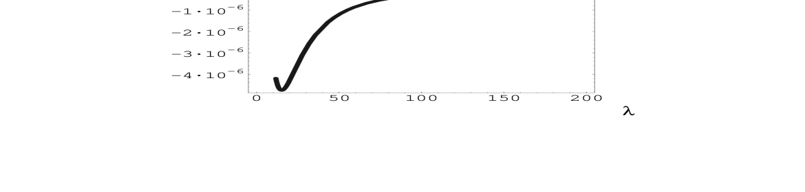
Figure 4: Ratio of $\frac{1}{8}\Delta P^{HH}_{tt}$ and $P_{\tiny\mbox{1-loop}}$ as a function of $11.65\leq\lambda\leq 200$.

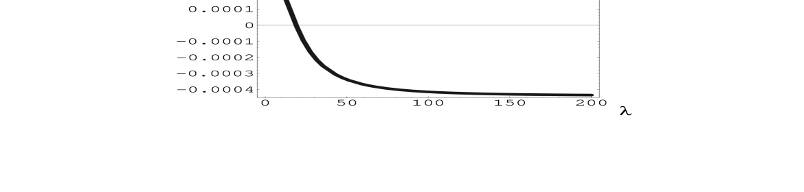
Figure 5: Ratio of $\frac{1}{8}\Delta P^{HM}_{tt}$ and $P_{\tiny\mbox{1-loop}}$ as a function of $11.65\leq\lambda\leq 200$.

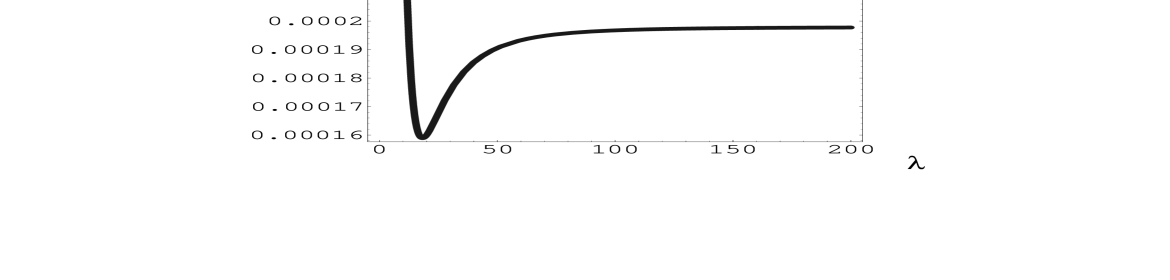
Figure 6: An upper bound for the modulus of the ratio of $\frac{1}{8}\Delta P^{HM}_{tv}$ and $P_{\tiny\mbox{1-loop}}$ as a function of $11.65\leq\lambda\leq 200$.

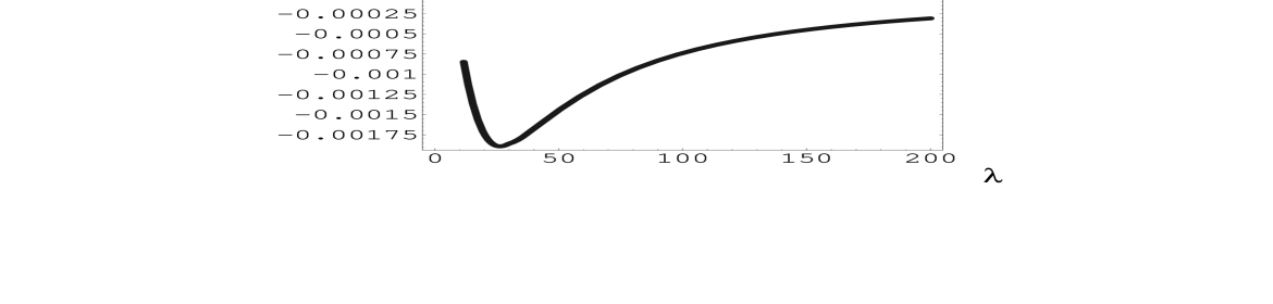
Figure 7: Ratio of $\frac{1}{4}\Delta P^{HHM}_{ttv}$ and $P_{\tiny\mbox{1-loop}}$ as a function of $11.65\leq\lambda\leq 200$.

Our computation indicates that the two-loop corrections are at most 0.2% of the one-loop result. The dominant contribution comes from the nonlocal diagram in Fig. 1.

7 Summary and Outlook

Our results can be summarized as follows: The picture of almost noninteracting thermal quasiparticles that was underlying the one-loop evolution of the effective coupling constant $e$ in the electric phase of a thermalized SU(2) Yang-Mills theory is confirmed by the two-loop calculation of the thermodynamical pressure. The (tiny) modification of the one-loop evolution equation for $e$ due to two-loop effects will be investigated in [12]. On a mesoscopic level this modification can be understood in terms of scattering processes off magnetic monopoles whose core size becomes comparable to the typical wave length $T^{-1}$ of a TLM mode for $T\searrow T_{c}$ where $T_{c}=\frac{\lambda_{c}\Lambda}{2\pi}=\frac{11.65\,\Lambda}{2\pi}$ denotes the critical temperature for the $2^{\tiny\mbox{nd}}$ order transition to the magnetic phase. For $T\gg T_{c}$ the magnetic charge of a monopole is too much smeared to be ’seen’ by the TLM mode. This simple fact arises from the constancy of $e$ for large temperatures and the core size or charge radius $R(T)$ of a monopole being approximately its inverse mass $M$ [1]

$$R(T)\sim M^{-1}(T)\sim e\sqrt{\frac{2\pi T}{\Lambda^{3}}}\,.$$ (37)

Thus the quick die-off of the two-loop correction to the pressure at large $T$ (compare with Figs. 4 through 7 and ignore the fact that our estimate for $\Delta P^{HM}_{tv}$, see Fig. 6, is too rough for large $T$ due to the omission of the vertex constraint and that a small infrared effect survives for large $T$ in Fig. 5 due to the masslessness of the TLM mode). The mechanical analogon for this situation is as follows: Imagine a box filled with heavy lead balls being at rest and light ping-pong balls moving around them. Now, switch on an interaction between the two species (wavelength of TLM mode becomes comparable to charge radius of monopole for $T\searrow T_{c}$). This will thermalize the system. However, the average momentum that is deprived from the ping-pong balls and added to the lead balls does not have an effect on the partial thermodynamical pressure of the latter since their momenta only probe the exponential tail of their Bose distribution. On the other hand, a decrease of the average ping-pong-ball momentum sizeably decreases their partial thermodynamical pressure. This is seen in Fig. 7 by the (negative!) dip of the dominating two-loop correction.

Despite the large value of $e\sim 5.1$ the smallness of two-loop corrections emerges from the existence of compositeness constraints which in turn are derived from the existence of a nontrivial ground state. We expect no major complications when generalizing our computation to SU(N). The situation is somewhat reminiscent of ${\cal N}=2$ supersymmetric Yang-Mills theory where the perturbative $\beta$ function for the gauge coupling is exact at one loop [13]. The important conceptual difference is that the one-loop exactness in the supersymmetric case is inforced by a strong symmetry while in our approach to the ${\cal N}=0$ Yang-Mills theory the identification of the essential degrees of freedom makes the interactions thereof almost vanish. We expect that the loop expansion of the thermodynamical pressure of an SU(N) Yang-Mills theory is not asymptotic but converges very quickly.

An important application of our results arises: If the photon is generated by an SU(2) Yang-Mills theory of Yang-Mills scale $\Lambda\sim T_{\tiny\mbox{CMB}}\sim 10^{-4}\,$eV being at the boundary between the magnetic and electric phases but on the magnetic side then light, being released at the time of decoupling of the CMB (deep within the electric phase of SU(2)${}_{\tiny\mbox{CMB}}$), must have travelled through a ’lattice’ of scattering centers (dual magnetic, that is, electrically charged monopoles) shortly before the Universe settled into the CMB dip where the monopoles are condensed into a classical field [1]. This effect is seen in Fig. 7 by a decrease of the dominating two-loop correction to the pressure for $T$ approaching $T_{c}$ (that is $T_{\tiny\mbox{CMB}}$) from above. The observable effect should be a cosmic Laue diagram with a large quadrupole contribution and manifest itself in terms of a large-angle ’anomaly’ in the power spectrum of temperature fluctuations in the cosmic microwave background. Such an ’anomaly’ indeed has been reported by the WMAP collaboration [10].

Appendix

Here we evaluate the contractions of the tensor structures as they appear in Eqs. (6) and (7). Exploiting Eq. (17), the contractions for local contributions are:
(1) Local, TLH-TLH:

$$\Gamma_{[4]abcd}^{\mu\nu\rho\sigma}\delta_{ab}\tilde{D}_{\mu\nu}(p)\delta_{cd}\tilde{D}_{\rho\sigma}(k)=-ie^{2}[\epsilon_{abe}\epsilon_{cde}(g^{\mu\rho}g^{\nu\sigma}-g^{\mu\sigma}g^{\nu\rho})+$$ (38)

$$\epsilon_{ace}\epsilon_{bde}(g^{\mu\nu}g^{\rho\sigma}-g^{\mu\sigma}g^{\nu\rho})+\epsilon_{ade}\epsilon_{bce}(g^{\mu\nu}g^{\rho\sigma}-g^{\mu\rho}g^{\nu\sigma})]\times$$

$$\delta_{ab}\left(g_{\mu\nu}-\frac{p_{\mu}p_{\nu}}{m^{2}}\right)\delta_{cd}\left(g_{\rho\sigma}-\frac{k_{\rho}k_{\sigma}}{m^{2}}\right)$$

$$= -ie^{2}\epsilon_{ace}\epsilon_{ace}\big{[}2g^{\mu\nu}g^{\rho\sigma}-g^{\mu\sigma}g^{\nu\rho}-g^{\mu\rho}g^{\nu\sigma}\big{]}\times$$

$$\Big{(}g_{\mu\nu}-\frac{p_{\mu}p_{\nu}}{m^{2}}\Big{)}\Big{(}g_{\rho\sigma}-\frac{k_{\rho}k_{\sigma}}{m^{2}}\Big{)}$$

$$= -2ie^{2}\left(24-6\frac{p^{2}}{m^{2}}-6\frac{k^{2}}{m^{2}}+2\frac{p^{2}k^{2}}{m^{4}}-2\frac{(pk)^{2}}{m^{4}}\right)\,.$$

(2) Local, TLH-TLM:

$$\Gamma_{[4]abcd}^{\mu\nu\rho\sigma}\delta_{ab}\tilde{D}_{\mu\nu}(p)\delta_{cd}\bar{D}_{\rho\sigma}(k)=-ie^{2}[\epsilon_{abe}\epsilon_{cde}(g^{\mu\rho}g^{\nu\sigma}-g^{\mu\sigma}g^{\nu\rho})+$$ (39)

$$\epsilon_{ace}\epsilon_{bde}(g^{\mu\nu}g^{\rho\sigma}-g^{\mu\sigma}g^{\nu\rho})+\epsilon_{ade}\epsilon_{bce}(g^{\mu\nu}g^{\rho\sigma}-g^{\mu\rho}g^{\nu\sigma})]\times$$

$$\delta_{ab}\left(g_{\mu\nu}-\frac{p_{\mu}p_{\nu}}{m^{2}}\right)\delta_{cd}\bar{D}_{\rho\sigma}(k)$$

$$= -ie^{2}\epsilon_{ace}\epsilon_{ace}\big{[}2g^{\mu\nu}g^{\rho\sigma}-g^{\mu\sigma}g^{\nu\rho}-g^{\mu\rho}g^{\nu\sigma}\big{]}\times$$

$$\Big{(}g_{\mu\nu}-\frac{p_{\mu}p_{\nu}}{m^{2}}\Big{)}\bar{D}_{\rho\sigma}(k)$$

$$= -2ie^{2}\left(-12+4\frac{p^{2}}{m^{2}}+2\frac{{\bf p}^{2}\sin^{2}{\theta}}{m^{2}}\right)\,.$$

In Eq. (39) $\theta$ denotes the angle between ${\bf p}$ and ${\bf k}$. For the nonlocal diagram we obtain:

$$\Gamma_{[3]abc}^{\lambda\mu\nu}(p,k,q)\Gamma_{[3]rst}^{\rho\sigma\tau}(p,k,q)\delta_{ar}\tilde{D}_{\lambda\rho}(p)\delta_{bs}\tilde{D}_{\mu\sigma}(k)\delta_{ct}\bar{D}_{\nu\tau}(q)$$ (40)

$$= e^{2}\epsilon_{abc}\epsilon_{rst}\big{[}g^{\lambda\mu}(p-k)^{\nu}+g^{\mu\nu}(k-q)^{\lambda}+g^{\nu\lambda}(q-p)^{\mu}\big{]}\times$$

$$\big{[}g^{\rho\sigma}(p-k)^{\tau}+g^{\sigma\tau}(k-q)^{\rho}+g^{\tau\rho}(q-p)^{\sigma}\big{]}\times$$

$$\delta_{ar}\delta_{bs}\delta_{ct}\Big{(}g_{\lambda\rho}-\frac{p_{\lambda}p_{\rho}}{m^{2}}\Big{)}\Big{(}g_{\mu\sigma}-\frac{k_{\mu}k_{\sigma}}{m^{2}}\Big{)}\bar{D}_{\nu\tau}(q)\,.$$

For not loosing track, we split the calculation into terms $\propto e^{2}$, $\propto\frac{e^{2}}{m^{2}}$ and $\propto\frac{e^{2}}{m^{4}}$ and keep $\bar{D}$ uncontracted in a first step. The contraction of structure constants $\epsilon_{ab3}\epsilon_{ab3}$ gives an additional factor 2.
Term $\propto 2e^{2}$:

$$\big{[}g^{\lambda\mu}(p-k)^{\nu}+g^{\mu\nu}(k-q)^{\lambda}+g^{\nu\lambda}(q-p)^{\mu}\big{]}\big{[}g^{\rho\sigma}(p-k)^{\tau}+$$ (41)

$$g^{\sigma\tau}(k-q)^{\rho}+g^{\tau\rho}(q-p)^{\sigma}\big{]}g_{\lambda\rho}g_{\mu\sigma}\bar{D}_{\nu\tau}(q)$$

$$= \big{[}g_{\rho\sigma}(p-k)^{\nu}+g_{\sigma}^{\nu}(k-q)_{\rho}+g^{\nu}_{\rho}(q-p)_{\sigma}\big{]}\times$$

$$\big{[}g^{\rho\sigma}(p-k)^{\tau}+g^{\sigma\tau}(k-q)^{\rho}+g^{\tau\rho}(q-p)^{\sigma}\big{]}\bar{D}_{\nu\tau}(q)$$

$$= \big{[}4(p-k)^{\nu}(p-k)^{\tau}+(p-k)^{\nu}(k-q)^{\tau}+(p-k)^{\nu}(q-p)^{\tau}+$$

$$(k-q)^{\nu}(p-k)^{\tau}+(k-q)^{2}g^{\nu\tau}+(q-p)^{\nu}(k-q)^{\tau}+$$

$$(q-p)^{\nu}(p-k)^{\tau}+(k-q)^{\nu}(q-p)^{\tau}+(q-p)^{2}g^{\nu\tau}\big{]}\bar{D}_{\nu\tau}(q)$$

$$= \big{[}2p^{\nu}p^{\tau}+2k^{\nu}k^{\tau}-6p^{\nu}k^{\tau}+(q-p)^{2}g^{\nu\tau}+(k-q)^{2}g^{\nu\tau}\big{]}\bar{D}_{\nu\tau}(q)$$

$$= 2\Big{(}{\bf p}^{2}-\frac{({\bf p}{\bf q})^{2}}{|{\bf q}|^{2}}\Big{)}+2\Big{(}{\bf k}^{2}-\frac{({\bf k}{\bf q})^{2}}{|{\bf q}|^{2}}\Big{)}-6\Big{(}{\bf p}{\bf k}-\frac{({\bf p}{\bf q})({\bf k}{\bf q})}{|{\bf q}|^{2}}\Big{)}-$$

$$2(q-p)^{2}-2(k-q)^{2}\,.$$

Terms proportional to $q^{\nu}$ or $q^{\tau}$ have been omitted after the second-last equal sign in Eq. (41) because, when contracted with $\bar{D}_{\nu\tau}(q)$, they vanish. Again, using Eq. (17) the expression after the last equal sign in Eq. (41) easily follows.
Next we look at the two terms proportional to $2\frac{e^{2}}{m^{2}}$ (compare with Eq. (40)).
The first one is:

$$\big{[}g^{\lambda\mu}(p-k)^{\nu}+g^{\mu\nu}(k-q)^{\lambda}+g^{\nu\lambda}(q-p)^{\mu}\big{]}\big{[}g^{\rho\sigma}(p-k)^{\tau}+$$ (42)

$$g^{\sigma\tau}(k-q)^{\rho}+g^{\tau\rho}(q-p)^{\sigma}\big{]}g_{\lambda\rho}k_{\mu}k_{\sigma}\bar{D}_{\nu\tau}(q)$$

$$= \big{[}k_{\rho}k_{\sigma}(p-k)^{\nu}+k^{\nu}k_{\sigma}(k-q)_{\rho}+k(q-p)g^{\nu}_{\rho}k_{\sigma}\big{]}\times$$

$$\big{[}g^{\rho\sigma}(p-k)^{\tau}+g^{\sigma\tau}(k-q)^{\rho}+g^{\tau\rho}(q-p)^{\sigma}\big{]}\bar{D}_{\nu\tau}(q)$$

$$= \big{[}k^{2}(p-k)^{\nu}(p-k)^{\tau}+k(k-q)(p-k)^{\nu}k^{\tau}+k(q-p)(p-k)^{\nu}k^{\tau}+$$

$$k(k-q)k^{\nu}(p-k)^{\tau}+(k-q)^{2}k^{\nu}k^{\tau}+k(q-p)k^{\nu}(k-q)^{\tau}+$$

$$k(q-p)k^{\nu}(p-k)^{\tau}+k(q-p)(k-q)^{\nu}k^{\tau}+[k(q-p)]^{2}g^{\nu\tau}\big{]}\bar{D}_{\nu\tau}(q)$$

$$= [k^{2}p^{\nu}p^{\tau}+q^{2}k^{\nu}k^{\tau}-2(kp)p^{\nu}k^{\tau}+[k(q-p)]^{2}g^{\nu\tau}\big{]}\bar{D}_{\nu\tau}(q)$$

$$= k^{2}\Big{(}{\bf p}^{2}-\frac{({\bf p}{\bf q})^{2}}{|{\bf q}|^{2}}\Big{)}+q^{2}\Big{(}{\bf k}^{2}-\frac{({\bf k}{\bf q})^{2}}{|{\bf q}|^{2}}\Big{)}-2pk\Big{(}{\bf p}{\bf k}-\frac{({\bf p}{\bf q})({\bf k}{\bf q})}{|{\bf q}|^{2}}\Big{)}$$

$$-2[k(q-p)]^{2}\,.$$

The second term $\propto 2\frac{e^{2}}{m^{2}}$ either is obtained by a direct calculation or by just exchanging $p\leftrightarrow k$ in Eq. (42):

$$\big{[}g^{\lambda\mu}(p-k)^{\nu}+g^{\mu\nu}(k-q)^{\lambda}+g^{\nu\lambda}(q-p)^{\mu}\big{]}\big{[}g^{\rho\sigma}(p-k)^{\tau}+$$ (43)

$$g^{\sigma\tau}(k-q)^{\rho}+g^{\tau\rho}(q-p)^{\sigma}\big{]}g_{\mu\sigma}p_{\lambda}p_{\rho}\bar{D}_{\nu\tau}(q)$$

$$= p^{2}\Big{(}{\bf k}^{2}-\frac{({\bf k}{\bf q})^{2}}{|{\bf q}|^{2}}\Big{)}+q^{2}\Big{(}{\bf p}^{2}-\frac{({\bf p}{\bf q})^{2}}{|{\bf q}|^{2}}\Big{)}-2pk\Big{(}{\bf p}{\bf k}-\frac{({\bf p}{\bf q})({\bf k}{\bf q})}{|{\bf q}|^{2}}\Big{)}-$$

$$2[p(q-k)]^{2}\,.$$

Finally, the term $\propto 2\frac{e^{2}}{m^{4}}$ is given by

$$\big{[}g^{\lambda\mu}(p-k)^{\nu}+g^{\mu\nu}(k-q)^{\lambda}+g^{\nu\lambda}(q-p)^{\mu}\big{]}\big{[}g^{\rho\sigma}(p-k)^{\tau}+$$ (44)

$$g^{\sigma\tau}(k-q)^{\rho}+g^{\tau\rho}(q-p)^{\sigma}\big{]}p_{\lambda}p_{\rho}k_{\mu}k_{\sigma}\bar{D}_{\nu\tau}(q)$$

$$= \big{[}(pk)p_{\rho}k_{\sigma}(p-k)^{\nu}+p(k-q)p_{\rho}k_{\sigma}k^{\nu}+k(q-p)p_{\rho}k_{\sigma}p^{\nu}\big{]}\times$$

$$\big{[}g^{\rho\sigma}(p-k)^{\tau}+g^{\sigma\tau}(k-q)^{\rho}+g^{\tau\rho}(q-p)^{\sigma}\big{]}\bar{D}_{\nu\tau}(q)$$

$$= \big{[}(pk)(p-k)^{\nu}+[p(k-q)]k^{\nu}+[k(q-p)]p^{\nu}\big{]}$$

$$\big{[}(pk)(p-k)^{\tau}+[p(k-q)]k^{\tau}+[k(q-p)]p^{\tau}\big{]}\bar{D}_{\nu\tau}(q)$$

$$= \big{[}(kq)^{2}p^{\nu}p^{\tau}+(pq)^{2}k^{\nu}k^{\tau}-2(pq)(kq)p^{\nu}k^{\tau}\big{]}\bar{D}_{\nu\tau}(q)$$

$$= (kq)^{2}\Big{(}{\bf p}^{2}-\frac{({\bf p}{\bf q})^{2}}{|{\bf q}|^{2}}\Big{)}+(pq)^{2}\Big{(}{\bf k}^{2}-\frac{({\bf k}{\bf q})^{2}}{|{\bf q}|^{2}}\Big{)}-$$

$$2(pq)(kq)\Big{(}{\bf p}{\bf k}-\frac{({\bf p}{\bf q})({\bf k}{\bf q})}{|{\bf q}|^{2}}\Big{)}\,.$$

Now, adding up Eqs.(41) through (44) (taking care of the correct signs), we have

Eq.(40) $$= 2e^{2}\left[\mbox{Eq.(\ref{eqn:HHMcontraction1})}-\mbox{Eq.(\ref{eqn:HHMcontraction2})}-\mbox{Eq.(\ref{eqn:HHMcontraction3})}+\mbox{Eq.(\ref{eqn:HHMcontraction4})}\right]$$ (45)

$$= 2e^{2}\Big{\{}2\frac{[p(q-k)]^{2}}{m^{2}}+\frac{2[k(q-p)]^{2}}{m^{2}}-2(q-p)^{2}-2(k-q)^{2}+$$

$$[2-\frac{k^{2}}{m^{2}}-\frac{q^{2}}{m^{2}}+\frac{(kq)^{2}}{m^{4}}]\Big{(}{\bf p}^{2}-\frac{({\bf p}{\bf q})^{2}}{|{\bf q}|^{2}}\Big{)}+$$

$$[2-\frac{q^{2}}{m^{2}}-\frac{p^{2}}{m^{2}}+\frac{(pq)^{2}}{m^{4}}]\Big{(}{\bf k}^{2}-\frac{({\bf k}{\bf q})^{2}}{|{\bf q}|^{2}}\Big{)}-$$

$$[6-4\frac{pk}{m^{2}}+2\frac{(pq)(kq)}{m^{4}}]\Big{(}{\bf p}{\bf k}-\frac{({\bf p}{\bf q})({\bf k}{\bf q})}{|{\bf q}|^{2}}\Big{)}\Big{\}}\,.$$

Using momentum conservation at the vertices, that is $q=-p-k$, we find:

$$\Big{(}{\bf p}^{2}-\frac{({\bf p}{\bf q})^{2}}{|{\bf q}|^{2}}\Big{)}=\Big{(}{\bf k}^{2}-\frac{({\bf k}{\bf q})^{2}}{|{\bf q}|^{2}}\Big{)}=-\Big{(}{\bf p}{\bf k}-\frac{({\bf p}{\bf q})({\bf k}{\bf q})}{|{\bf q}|^{2}}\Big{)}=\frac{{\bf p}^{2}{\bf k}^{2}\sin^{2}{\theta}}{({\bf p}+{\bf k})^{2}}\,.$$ (46)

And thus,
(3) Nonlocal, TLH-TLH-TLM:

$$\Gamma_{[3]abc}^{\lambda\mu\nu}(p,k,q)\Gamma_{[3]abc}^{\rho\sigma\tau}(-p,-k,-q)\tilde{D}_{\lambda\rho}(p)\tilde{D}_{\mu\sigma}(k)\bar{D}_{\nu\tau}(q)$$ (47)

$$= 2e^{2}\Big{[}10p^{2}+10k^{2}+16pk-2\frac{k^{4}}{m^{2}}-2\frac{p^{4}}{m^{2}}-8\frac{p^{2}(pk)}{m^{2}}-8\frac{k^{2}(pk)}{m^{2}}-$$

$$16\frac{(pk)^{2}}{m^{2}}-\frac{{\bf p}^{2}{\bf k}^{2}\sin^{2}{\theta}}{(p+k)^{2}}\Big{(}10-3\frac{p^{2}}{m^{2}}-3\frac{k^{2}}{m^{2}}-8\frac{pk}{m^{2}}+\frac{p^{4}}{m^{4}}+$$

$$\frac{k^{4}}{m^{4}}+4\frac{p^{2}(pk)}{m^{4}}+4\frac{k^{2}(pk)}{m^{4}}+4\frac{(pk)^{2}}{m^{4}}+2\frac{p^{2}k^{2}}{m^{4}}\Big{)}\Big{]}\,.$$

Here, we have used the fact that $\Gamma(-p,-k,-q)=-\Gamma(p,k,q)$.