Propagators on One-Loop Worldsheets for Supersymmetric Orientifolds and Intersecting Branes

Abstract:

We obtain the one-loop propagators in superstring theory for the general case when the worldsheet fields satisfy non-trivial holonomy and/or boundary conditions. Non-trivial holonomy arises in orbifold and orientifold backgrounds whereas non-trivial boundary conditions arise in backgrounds containing D-branes of different dimensionality or D-branes intersecting each other at an angle. In our derivation, we use a generalized version of the method of images. Dihedral groups play a crucial role in constructing the one-loop propagators.

1 Introduction

Perturbative string theory is defined in terms of a sum over worldsheets of different topology. However, the choice of a particular topology alone does not fix the path integral completely. Instead, whenever a given worldsheet contains non-contractible loops, one has to specify the holonomy of the conformal fields living on the worldsheet. Also, if a worldsheet contains boundaries, one has to specify boundary conditions. Depending on the string theory background under consideration, there can be more than one possible choice for holonomy and boundary conditions for a given worldsheet. In this case, one has to sum over all these contributions. Non-trivial holonomy arises in orbifold and orientifold backgrounds where, if one works in the covering space, the holonomy group for the bosonic string coordinates on any given worldsheet is a subgroup of the orbifold group. Non-standard boundary conditions arise for backgrounds containing D-branes of different dimensionality or D-branes intersecting each other at an angle. Taken together, these configurations are the object of a large part of the existing literature on string theory backgrounds.

One of the guiding principles in studying string theory backgrounds has been the search for quasi-realistic backgrounds, i.e. backgrounds whose low-energy limit is similar to the (Minimal Supersymmetric) Standard Model or a GUT extension thereof. In this respect, models with intersecting D-branes or D-branes at orbifold singularities have been particularly successful (for reviews, see [1, 2]). The essential tool for investigating the low-energy behaviour of a given string theory background is the low-energy effective action which can be obtained by computing string scattering amplitudes, i.e. using the S-matrix approach [3]. At tree-level, the four-dimensional effective action can be obtained by dimensional reduction from the ten-dimensional supergravity action. In the absence of fluxes, it typically contains a large number of moduli. These can partially be fixed by introducing fluxes on the internal cycles of a warped Calabi-Yau compactification [4]. Non-perturbative effects have been evoked to achieve complete moduli stabilization within the framework of flux compactifications [5]. However, it remains an open question how perturbative corrections change the picture.

Computing string scattering amplitudes in the untwisted NS-NS sector basically requires knowledge of three quantities: the vertex operators for creating and annihilating asymptotic states, the vacuum path integral and the propagators of the worldsheet fields. The vertex operators are completely determined by the local properties of the underlying CFT and are unaffected by the choice of topology, holonomy and boundary conditions. On the other hand, the effect of non-trivial holonomy on the vacuum amplitude is familiar from the computation of tadpole cancellation conditions in orientifold backgrounds. There, non-trivial holonomy is taken into account by including twisted string sectors and/or inserting twists in the partition function’s trace [7, 8, 9, 10, 11, 12, 13]. Non-standard boundary conditions affect the partition function simply by modifying the open string spectrum. It remains to determine the worldsheet propagators for non-trivial holonomy and boundary conditions. To fill in this gap is the purpose of this article.

The method of images is a powerful tool for computing string theory scattering amplitudes. It has been used to derive expressions for propagators on tree-level and one-loop worldsheets with trivial holonomy and boundary conditions [14] and also in direct (tree-level) computations of tadpoles in type-I string theory [15]. In section 2, we review the method of images as applied to the computation of the standard propagators on one-loop worldsheets and outline how to generalize this method in order to derive propagators satisfying generic holonomy and boundary conditions. In section 3, we apply the generalized method of images and obtain explicit expressions for the propagators. In section 4, we discuss applications of our results and comment on an extension of our methods to the R-R and R-NS sectors.

2 The method of images

The one-loop surfaces are the torus, the annulus, the Klein bottle and the Möbius strip ($\mathcal{T},\mathcal{A},\mathcal{K}$ and $\mathcal{M}$). The latter three can be obtained from a covering torus by identifying points under an antiholomorphic involution $\mathcal{I}$. This fact has been used to construct the corresponding propagators with trivial holonomy and NN-boundary conditions by employing the method of images [14, 16]. We normalize the torus such that $\mathcal{T}=\mathbb{C}/(\mathbb{Z}+\tau\mathbb{Z})$. Then, table 1 summarizes the geometrical construction of $\mathcal{A}$, $\mathcal{K}$ and $\mathcal{M}$ where we choose the respective fundamental domain such that the familiar picture of tubes connecting D-branes and O-planes becomes obvious. In the case of the Klein bottle, the ‘loop channel’ picture is recovered by using the fundamental domain $\mathcal{K}=[0,1]\times i[0,t]$ instead, whereas for the Möbius strip one has to use $\mathcal{M}=[0,1/2]\times i[0,t/2]$. Here, t denotes the canonically normalized loop channel proper time (see e.g. [17]), i.e. Klein bottle, annulus and Möbius strip contribute to the vacuum amplitude through the terms

$$\mathcal{Z}_{\mathcal{K}}=\int_{0}^{\infty}\frac{dt}{2t}\operatorname{Tr}_{cl}\left(\Omega e^{-H_{cl}t}\right);\quad\mathcal{Z}_{\mathcal{A}}=\int_{0}^{\infty}\frac{dt}{2t}\operatorname{Tr}_{o}\left(e^{-H_{o}t}\right);\quad\mathcal{Z}_{\mathcal{M}}=\int_{0}^{\infty}\frac{dt}{2t}\operatorname{Tr}_{o}\left(\Omega e^{-H_{o}t}\right)$$ (1)

respectively where the trace is either over open or closed string states, $\Omega$ denotes worldsheet orientation reversal and we implicitly assume implementation of the GSO-projection. The propagators for trivial holonomy and NN-boundary conditions can be obtained by symmetrizing the propagator on the covering torus under the involution $\mathcal{I}$ and restricting to a fundamental domain of the derived surface. Equivalently, we can say that for every charge $q$ at a point $z$, one places an identical mirror charge $q$ at $\mathcal{I}(z)$.

	$\mathcal{I}(z)$	$\tau$	$\mathcal{F}$
$\mathcal{A}$	$-\overline{z}$	$it/2$	$[0,1/2]\times i[0,t/2]$
$\mathcal{K}$	$-\overline{z}+\tau/2$	$2it$	$[0,1/2]\times i[0,2t]$
$\mathcal{M}$	$-\overline{z}$	$it/2+1/2$	$[1/2,3/4]\times i[0,t]$

Table 1: The involution $\mathcal{I}$, complex structure $\tau$ of the covering torus and fundamental domain $\mathcal{F}$ for the surfaces $\mathcal{A}$, $\mathcal{K}$ and $\mathcal{M}$ respectively. The variable ‘t’ is the canonically normalized loop modulus

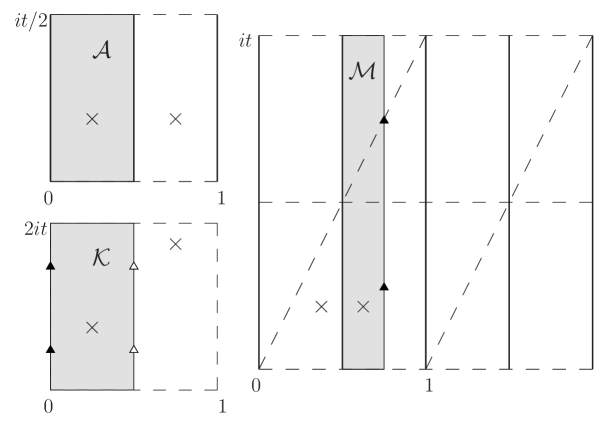
Figure 1: the annulus, Möbius strip and Klein bottle and their respective covering tori. Bold lines mark boundaries, triangles are to be identified and the x’s mark a charge and the corresponding mirror charge.

2.1 Boson propagators

We generalize the method of images to cover general holonomy as well as non-trivial boundary conditions. The general strategy is the following: For a given worldsheet, we pick a minimal set of closed loops generating the fundamental group. The transformations of the worldsheet fields when transported along these loops generate the holonomy group $G$. We differentiate between the abstract group $G$ and its defining spacetime representation which we denote by $R$. Then, if we can find a representation $f$ of $G$, acting on a torus $\mathcal{T}$, we automatically get an induced representation of $G$ which acts on the worldsheet fields $X$ living on $\mathcal{T}$:

$$g:X^{i}\mapsto(R_{g})^{i}_{\phantom{i}j}X^{j}\circ f_{g}^{-1}.$$ (2)

Generally, identifying points on the torus under the action of $G$ introduces additional closed loops. Furthermore, $G$-invariant worldsheet fields pick up a spacetime transformation $R_{g}$ when running around the closed loop associated to $g$:

$$X(f_{g}(z,\overline{z}))=R_{g}X(z,\overline{z})$$ (3)

Thus, by symmetrizing the torus propagator under $G$, we can specifically tailor propagators satisfying a given set of holonomy conditions when regarded as functions over $\mathcal{T}/G$. Finally, by choosing an appropriate representation $f$ of $G$, we ensure that $\mathcal{T}/G$ represents the correct worldsheet. Generally, we use both holomorphic and antiholomorphic transformations $f_{g}$. While holomorphic transformations induce orientation-preserving loops, antiholomorphic transformations may induce orientation-reversing loops (i.e. cross-caps) and boundaries. The latter arise if there are fix points under $f_{g}$. In order to deal with worldsheets with boundaries, we have to further extend the method described so far. Consider a boundary $b$ and a D-brane $D_{b}$ which encodes the boundary conditions on $b$. A crucial observation is the following: If $b$ is given by the fixed point locus of a transformation $f_{b}$ acting on a suitable covering torus, the boundary conditions on $b$ are equivalent to invariance of the worldsheet fields $X$ under the transformation

$$b:X^{i}\mapsto(R_{b})^{i}_{\phantom{i}j}X^{j}\circ f_{b}^{-1}$$ (4)

where $R_{b}$ is a spacetime reflection about $D_{b}$. This will be explained in section 3.3 when we discuss the annulus worldsheet in detail. Thus, by symmetrizing the torus propagator under (4), we enforce the correct boundary conditions at $b$. We are led to the following recipe for obtaining propagators on a one-loop surface $\sigma$:

• Pick a set of $n$ closed loops which generate the fundamental group of $\sigma$. Let $g_{1},\dots,g_{n}$ denote the holonomy transformations along these loops. Also, for each of $m$ boundaries, define a D-brane encoding the boundary conditions and let $b_{1},\dots,b_{m}$ denote reflections about the respective D-brane.

• Define $G=\langle g_{1},\dots,g_{n},b_{1},\dots,b_{m}\rangle$. We might call this the generalized holonomy group as it encodes information about the holonomy as well as boundary conditions. Find a representation of $G$ on a suitable torus $\mathcal{T}$ such that $\sigma=\mathcal{T}/G$.

• Symmetrize the torus propagator under the induced action of $G$ and restrict to a fundamental domain of $\sigma$.

Finally, note that the second step is not always possible as in special cases a given worldsheet $\sigma$ cannot be represented as $\mathcal{T}/G$. As we will see in section 3, this obstruction does indeed occur if one includes fermionic fields in the analysis. However, we can solve this problem by a minor modification of our method. Namely, we can always choose a larger group $H$, such that $\sigma=\mathcal{T}/H$ and $G=H/N$ where $N$ is a normal subgroup of $H$. In this case, the spacetime representation of $G$ induces a spacetime representation of $H$ and therefore we get a representation of $H$ on the worldsheet fields. Consequently, the propagators on $\sigma$ are obtained by symmetrizing the torus propagator under $H$.

2.2 Fermion propagators

For the fermionic worldsheet fields $\Psi^{M}(z,\overline{z})=(\psi^{M}(z),\tilde{\psi}^{M}(\overline{z}))$, we have to allow for a transformation of the spinor indices when going around closed loops, in addition to any transformation of the spacetime indices. This means that the holonomy group $\tilde{G}$ for the fermions is generated by transformations

$${\tilde{g}}:\Psi^{i}\mapsto(R_{\tilde{g}})^{i}_{\phantom{i}j}A_{\tilde{g}}\Psi^{j}$$ (5)

where $A$ is a real two-by-two matrix representation of $\tilde{G}$ acting on the spinor indices and $R:{\tilde{g}}\mapsto R_{\tilde{g}}$ is a group homomorphism mapping $\tilde{G}$ to the corresponding holonomy group $G$ for bosonic fields. In analogy to the bosonic case, we represent $\tilde{G}$ on a suitable covering torus $\mathcal{T}$ such that $\mathcal{T}/\tilde{G}$ reproduces the surface of interest. Then, the fermion propagator is obtained by symmetrizing the torus propagator under the following action of $\tilde{G}$:

$${\tilde{g}}:\Psi^{i}\mapsto(R_{\tilde{g}})^{i}_{\phantom{i}j}(A_{\tilde{g}}\Psi)^{j}\circ f_{\tilde{g}}^{-1},$$ (6)

where $f$ denotes the representation of $\tilde{G}$ on $\mathcal{T}$. We will use the Pauli matrices to construct more explicit expressions for the fermion propagators. For these, we use the following conventions:

$$\tau_{1}=\begin{pmatrix}0&+1\\ +1&0\end{pmatrix},\qquad\tau_{2}=\begin{pmatrix}0&-i\\ +i&0\end{pmatrix},\qquad\tau_{3}=\begin{pmatrix}+1&0\\ 0&-1\end{pmatrix}.$$ (7)

For a given holonomy group $G$ of the bosonic fields, the group $\tilde{G}$ is severely constrained by the requirement of Lorentz-invariance of the RNS action. Going around an orientation-preserving closed loop, both components of $\Psi$ have to return to themselves up to the action of some $R_{\tilde{g}}\in G$ plus a possible sign change which can be assigned to the left- and right-moving component independently. Therefore, we find that $A_{\tilde{g}}\in\{\pm\mathbf{1},\pm\tau_{3}\}$. On the other hand, going around an orientation-reversing loop relates the left-moving to the right-moving component. Since going around the loop twice gives an orientation-preserving loop, the corresponding spinor transformation has to square to one of the matrices in $\{\pm\mathbf{1},\pm\tau_{3}\}$. It follows that, if $\tilde{g}$ corresponds to an orientation-reversing loop, we have $A_{\tilde{g}}\in\{\pm\tau_{1},\pm i\tau_{2}\}$.. Finally, boundary conditions can be taken account of by using a generalized holonomy group in the sense of section 2.1. The transformation of the fermionic fields corresponding to a boundary $b$ (and a D-brane $D_{b}$) is restricted by 2-d supersymmetry and the requirement that boundary terms from varying the RNS action vanish. If $R_{b}$ is a reflection about the D-brane encoding boundary conditions at $b$, the fermionic fields have to satisfy $\Psi^{i}=(R_{b})^{i}_{\phantom{i}j}A_{b}\Psi^{j}$ on the boundary where $A_{b}=\pm\tau_{1}$. In particular, if we choose coordinates such that the D-brane is aligned with the coordinate-axes, this boundary condition reduces to the familiar relation $\psi=\pm\tilde{\psi}$. Altogether, we find that for $\tilde{g}$ in the generalized holonomy group, the fermionic fields satisfy

$$\Psi^{i}(f_{\tilde{g}}(z,\overline{z}))=(R_{\tilde{g}})^{i}_{\phantom{i}j}A_{\tilde{g}}\Psi^{j}(z,\overline{z})$$ (8)

where the possible choices for $A_{\tilde{g}}$ are summarized as follows:

$$A\in\begin{cases}\{\pm\mathbf{1},\pm\tau_{3}\}&\text{ for orientation-preserving loops}\\ \{\pm\tau_{1},\pm i\tau_{2}\}&\text{ for orientation-reversing loops}\\ \{\pm\tau_{1}\}&\text{ for boundaries}\end{cases}$$ (9)

In general, the choice of $A_{\tilde{g}}$ is further constrained by consistency with the fundamental group (for details, see section 3). The remaining choices for $A$ account for the possible spin structures on the respective surface. The RNS action is invariant under the global symmetry $\Psi\rightarrow\tau_{3}\Psi$ which changes the relative sign of left- and right-moving fermionic modes. In equation (8), this symmetry maps $\tau_{1}$ to $-\tau_{1}$ and $\tau_{2}$ to $-\tau_{2}$. In the simple examples of reference [14], only one antiholomorphic involution per worldsheet was needed whose corresponding sign could therefore be fixed. In the more general cases considered in this paper, this is no longer possible as the relative sign between spinor transformations associated to different antiholomorphic transformations matters. Only the overall sign can be fixed.

2.3 Propagators on covering tori

We consistently normalize worldsheets such that closed strings in the ‘loop channel’ have unit length whereas open strings have length $1/2$. In order to maintain this normalization we need covering tori of varying size. We use the following notation to denote tori with non-standard normalization:

$$\mathcal{T}^{(N,M)}\equiv\mathbb{C}/(N\mathbb{Z}+M\tau\mathbb{Z})$$ (10)

Throughout this paper we will refer to $\tau$ as the complex structure of $\mathcal{T}^{(N,M)}$. The bosonic propagator on such a torus is given by

$$\langle X^{i}(z,\overline{z})X^{j}(w,\overline{w})\rangle_{\mathcal{T}^{N,M}}=P^{ij}_{N,M}(z,w)=G^{ij}p_{N,M}(z,w)$$ (11)

where $G^{ij}$ is the spacetime metric and the scalar propagator $p_{N,M}$ is given by

$$p_{N,M}(z,w)\equiv-\frac{1}{4}\ln\left|\frac{\vartheta_{1}\left(\frac{z-w}{N}|\frac{M}{N}\tau\right)}{\vartheta^{\prime}_{1}\left(0|\frac{M}{N}\tau\right)}\right|^{2}+\frac{\pi}{2NM}\frac{(\operatorname{Im}z-\operatorname{Im}w)^{2}}{\operatorname{Im}\tau}.$$ (12)

It can easily be checked that this expression yields the correct pole structure and periodicity. Similarly, the fermion propagator for odd spin structure is given by

$$\langle\Psi^{i}(z,\overline{z})(\Psi^{j})^{tr}(w,\overline{w})\rangle_{\mathcal{T}^{N,M},\text{odd}}=S^{ij}_{N,M}(z,w)=G^{ij}s_{N,M}(z,w)$$ (13)

where $\Psi^{i}(z,\overline{z})=(\psi^{i}(z),\tilde{\psi}^{i}(\overline{z}))$ are the two-dimensional Majorana spinors, the transpose operation refers to the spinor indices and we define:

$$s_{N,M}\equiv P^{F}_{N,M}(z,w)\left(\frac{1+\tau_{3}}{2}\right)+P^{F}_{N,M}(\overline{z},\overline{w})\left(\frac{1-\tau_{3}}{2}\right)$$ (14)

$$P^{F}_{N,M}(z,w)\equiv-\frac{1}{4N}\frac{\vartheta_{1}^{\prime}\left(\frac{z-w}{N}\Large|\frac{M}{N}\tau\right)}{\vartheta_{1}\left(\frac{z-w}{N}\Large|\frac{M}{N}\tau\right)}-\frac{i\pi}{2NM}\frac{(\operatorname{Im}z-\operatorname{Im}w)}{\operatorname{Im}\tau}.$$ (15)

The bosonic propagator (11) along with the odd spin structure fermion propagator (13) are sufficient to express all other propagators in this paper. In particular, we derive expressions for even spin structure propagators on the torus using the method of images in appendix B and contrast them to the standard expressions.

3 Propagators on one-loop surfaces

In this section we derive the propagators for one-loop surfaces supporting fields with non-trivial holonomy and boundary conditions. As far as supersymmetric orientifolds are concerned, our results enjoy full generality, covering Abelian as well as non-Abelian orientifolds with generic spacetime action. There are a number of rather special cases, for which the propagators are already known. Propagators on all untwisted one-loop worldsheets have been constructed in references [14, 16]. In the appendix of reference [19], the fermion propagator on the twisted torus for Abelian orbifolds was given in terms of Jacobi functions with characteristics. For an orientifold group of the form $G\times\{1,\Omega\}$, where $G$ is an Abelian orbifold group, the propagators on some of the remaining one-loop worldsheets can be obtained from the twisted torus through a simple application of the method of images. This was also noted in reference [19], where propagators on the annulus and Möbius strip were constructed in this way and used to compute various matter field couplings in the four-dimensional effective action. However, this approach does not cover more general orientifold constructions. In particular, it does not cover the important orientifold constructions widely known as $\Omega J$-orientifolds and $\Omega\mathcal{R}$-orientifolds (these arise from orientifold groups of the form $G\times\mathbb{Z}_{2}$, where the $\mathbb{Z}_{2}$ combines worldsheet orientation reversal with an inversion of some of the spacetime coordinates). The fermion propagator on an annulus with DN-boundary conditions was also given in the appendix of [19]. In reference [20], the masses of anomalous $U(1)$ gauge fields in four-dimensional orientifolds were computed, using the propagators of reference [19]. We will start by considering the twisted torus which is the simplest non-trivial example and serves as an illustration of the generalized method of images which will be essential in deriving propagators for the remaining one-loop surfaces.

3.1 The Torus

We are interested in tori with non-trivial holonomy. These arise, for instance, in orbifolds of type II string theory on $\mathbb{R}^{1,3}\times T^{6}$. Recall that one constructs the orbifold spectrum in two steps: First, one obtains untwisted states by projecting the full spectrum onto the subspace of states which are invariant under some discrete spacetime symmetry $\mathcal{G}$. Then, one adds the twisted sector which consists of strings which close onto themselves only up to some symmetry transformation $g\in\mathcal{G}$. Correspondingly, in the topological worldsheet expansion, one has to add ‘twisted tori’ on which the worldsheet fields return to themselves up to the action of a symmetry group element. Since there are two independent closed loops on a torus, we can classify all tori by two twists, $g_{1}$ and $g_{2}$. For consistency, these have to be in a representation of the fundamental group $\mathbb{Z}\times\mathbb{Z}$ of the torus, i.e. any two twists appearing in the same worldsheet have to commute with each other. If we use the familiar parallelogram representation of the torus, the periodicity conditions for the bosonic worldsheet fields read:

$$X^{i}(z+1) =(g_{1})^{i}_{\phantom{i}j}X^{j}(z)$$ (16)

$$X^{i}(z+\tau) =(g_{2})^{i}_{\phantom{i}j}X^{j}(z)$$ (17)

For finite $\mathcal{G}$, we have $g_{1}^{N}=g_{2}^{M}=1$ for some integers $N$ and $M$ and therefore, the holonomy group $G$ is given by $\mathbb{Z}_{N}\times\mathbb{Z}_{M}$ (or a subgroup thereof). To obtain the propagator for the twisted torus, we start with an untwisted torus $\mathcal{T}^{(N,M)}$ [defined in equation (10)] on which we represent the action of $\mathbb{Z}_{N}\times\mathbb{Z}_{M}$ by translations along the lattice directions. Then, using the method of images, we find the propagator on the twisted torus:

$$\langle X^{i}(z,\overline{z})X^{j}(w,\overline{w})\rangle_{g_{1},g_{2}}=\sum_{n=0}^{N-1}\sum_{m=0}^{M-1}(g_{1}^{n}g_{2}^{m})^{i}_{\phantom{i}k}P_{N,M}^{kj}(z-n-m\tau,w)$$ (18)

It is easy to see that this expression satisfies the appropriate periodicity conditions. Furthermore, it inherits the correct pole structure from $P_{N,M}$. This procedure works for non-Abelian orbifold groups only because for a given worldsheet, $g_{1}$ and $g_{2}$ have to commute. Note that because of the fact that the torus propagator only depends on $z-w$ and moreover is an even function in $z-w$, we do not need to symmetrize in $w$ separately.

For the fermionic fields, we have additional freedom in choosing periodicity conditions. They satisfy

$$\Psi^{i}(z+1) =(g_{1})^{i}_{\phantom{i}j}A_{1}\Psi^{j}(z)$$ (19)

$$\Psi^{i}(z+\tau) =(g_{2})^{i}_{\phantom{i}j}A_{2}\Psi^{j}(z)$$ (20)

where $A_{i}\in\{\pm 1,\pm\tau_{3}\}$ acts on the spinor indices. Different choices for the matrices $A_{i}$ represent the 16 different spin structures $(s,\tilde{s})$ on the twisted torus. Without loss of generality, we can assume $N$ and $M$ to be even so that the fermionic fields can be analytically continued to doubly periodic fields on the covering torus $\mathcal{T}^{(N,M)}$. We should make it clear that this does not represent a restriction on the form of the orbifold group or its elements $g_{1}$ and $g_{2}$ as $N$ and $M$ are merely unspecified multiples of the order of $g_{1}$ and $g_{2}$ respectively. Since all $A_{i}$ mutually commute, we can write the fermion propagator as follows:

$$\langle\Psi^{i}(z,\overline{z})(\Psi^{tr})^{j}(w,\overline{w})\rangle_{g_{1},g_{2},(s,\tilde{s})}=\sum_{n=0}^{N-1}\sum_{m=0}^{M-1}(g_{1}^{n}g_{2}^{m})^{i}_{\phantom{i}k}A_{1}^{n}A_{2}^{m}S_{N,M}^{kj}(z-n-m\tau,w)$$ (21)

In appendix B, we show that this expression, when applied to an untwisted torus, reproduces the familiar even spin structure fermion propagators. As an application of the general expressions (18) and (21) for the boson and fermion propagators on a twisted torus, we consider Abelian orbifolds. More precisely, we assume that the six extra dimensions can be decomposed into pairs of coordinates, $\mathbf{X}^{i}\equiv{(X^{i},Y^{i}),\ i=1,2,3}$, such that the orbifold group acts on these as independent rotations by angles $\theta^{(i)}$ respectively. Then, the boson propagator takes block matrix form. Choose integers $N$ and $M$ such that $N\theta^{(1)}$ and $M\theta^{(2)}$ are multiples of $2\pi$. For a single pair of coordinates, we obtain the following expression:

$$\langle\mathbf{X}^{tr}(z,\overline{z})\mathbf{X}(w,\overline{w})\rangle_{\theta^{(1)},\theta^{(2)}}=\sum_{n=0}^{N-1}\sum_{m=0}^{M}R(n\theta^{(1)}+m\theta^{(2)})P_{N,M}(z-n-m\tau,w)$$ (22)

where $P_{N,M}$ is the boson propagator (11) in the form of a two-by-two matrix and $R(\theta)$ is the matrix representation of a rotation by an angle $\theta$. For the fermions, let $\mathbf{\Psi}^{i}$ denote the spacetime doublet corresponding to the bosonic coordinate $\mathbf{X}^{i}$. Then, the fermion propagator for a single pair of dimensions takes the form:

$$\langle\mathbf{\Psi}(z,\overline{z})\mathbf{\Psi}^{tr}(w,\overline{w})\rangle_{\theta^{(1)},\theta^{(2)},(s,\tilde{s})}=\sum_{n=0}^{N-1}\sum_{m=0}^{M-1}R(n\theta^{(1)}+m\theta^{(2)})A_{1}^{n}A_{2}^{m}S_{N,M}(z-n-m\tau,w)$$ (23)

where the transpose operation applies to both spinor and spacetime components and $S_{N,M}$ is the fermion propagator (13). Here, we suppress all indices with the understanding that $R(\theta)$ acts on spacetime indices while the $A_{i}$ act on the spinor indices. In appendix B, we compare this expression to the fermion propagator in reference [19] and establish equivalence between the two different expressions.

Finally, we would like to note that for supersymmetry-preserving orientifolds, we can continue to use expressions (22) and (23) after an appropriate coordinate transformation, even if the orbifold group is non-Abelian. (by ‘orbifold group’ we mean the subgroup of the orientifold group consisting of all pure spacetime transformations). All we needed was that the two group elements $g_{1}$ and $g_{2}$ could be written as independent rotations of the same three coordinate planes. Equivalently, if we complexify the extra six dimensions, we require that $g_{1}$ and $g_{2}$ are simultaneously diagonalizable by a unitary coordinate transformation. If the orientifold is to preserve at least $\mathcal{N}=1$ supersymmetry in four dimensions, the orbifold group has to be a discrete subgroup of the R-symmetry $SU(3)$. Each element of $SU(3)$ individually is unitarily diagonalizable. However, as noted above, compatibility with the fundamental group of the torus means that $g_{1}$ and $g_{2}$ have to commute and therefore they are simultaneously diagonalizable. For non-Abelian orbifolds, the unitary transformations which diagonalize a given group element will vary over the full orbifold group and hence the more general expressions (18) and (21) for the propagators on twisted tori might be more suitable for explicit computations than the respective specializations (22) and (23). On the other hand, for abelian orbifolds, one and the same unitary transformation diagonalizes all group elements.

3.2 The Klein Bottle

The Klein Bottle contains two independent loops along which the worldsheet fields can have non-trivial holonomy. As explained in section 2, the Klein Bottle can be obtained from a standard torus with complex structure $\tau=2it$ by identifying points under the antiholomorphic involution $\mathcal{I}_{K}:z\mapsto-\overline{z}+\tau/2$. For our purposes, the choice $\mathcal{K}=[0,1/2]\times i[0,2t]$ for the fundamental domain of the Klein Bottle is the most useful as it corresponds to a tube stretching between two cross-caps. If we consider an orientifold group of the form $\mathcal{G}+\Omega H$, then going around a cross-cap in a loop (e.g. going from $0$ to $it$ in our representation of the Klein bottle), a worldsheet field has to come back to itself up to some $g\in H$. In the spacetime picture, we find a corresponding O-plane. On the other hand, if in a given background, there are O-planes of different type, their interaction through exchange of closed strings is described by worldsheets whose cross-cap loops support a holonomy given by two different group elements, $g_{1}$ and $g_{2}$ respectively. These have to satisfy the consistency condition $g_{1}^{2}=g_{2}^{2}=h$ for some $h\in\mathcal{G}$ in order to be compatible with the fundamental group of the Klein bottle. Following the method of images as described in section 2, let us first determine the holonomy group $G$ which is generated by $g_{1}$ and $g_{2}$. First, notice that $h$ is in the centre of $G$. We can therefore construct the quotient group $G_{h}\equiv G/\langle h\rangle$. The equivalence classes $[g_{1}]$ and $[g_{2}]$ square to unity and satisfy $([g_{1}][g_{2}])^{p}=id_{G_{h}}$ for some integer $p$. These are the defining relations for the dihedral group $D_{p}$ (see appendix A), the symmetry group of a regular $p$-sided polygon and it follows that $G$ is a semidirect product, $G=\mathbb{Z}_{q}\rtimes D_{p}$ where $q$ is the order of $h$. Now, it is possible to find an appropriate group action of $G$ on the worldsheet of a rectangular torus $\mathcal{T}^{(p,q)}$ such that the Klein bottle is given by $\mathcal{T}^{(p,q)}/G$. We represent the twists $g_{1}$ and $g_{2}$ by the following antiholomorphic worldsheet transformations:

$$f_{1}:z\mapsto-\overline{z}+\frac{\tau}{2};\qquad\qquad f_{2}:z\mapsto 1-\overline{z}+\frac{\tau}{2}$$ (24)

Note that $f_{2}\circ f_{1}$ is a translation by $1+\tau$ whereas $f_{1}^{2}=f_{2}^{2}$ are simply translations by $\tau$. It is therefore easy to see that $f_{1}$ and $f_{2}$ generate a representation of $\mathbb{Z}_{q}\rtimes D_{p}$. In order to obtain the standard normalization for the Klein Bottle, we need to set the complex structure of the covering torus to $\tau=2it$. Then, if we choose the fundamental domain to be $\mathcal{K}=[0,1/2]\times i[0,2t]$, the edges $\operatorname{Re}z=0$ and $\operatorname{Re}z=1/2$ are cross-caps corresponding to $g_{1}$ and $g_{2}$ respectively. The bosonic propagator on the Klein bottle is given by:

$$\langle X^{i}(z,\overline{z}),X^{j}(w,\overline{w})\rangle_{g_{1},g_{2}}=\sum_{n=0}^{p-1}\sum_{m=0}^{q-1}\Big{\{}((g_{2}g_{1})^{n}h^{m})^{i}_{\phantom{i}k}P^{kj}_{p,q}(z+n-\tau(n+m),w)\\ +(g_{1}(g_{2}g_{1})^{n}h^{m})^{i}_{\phantom{i}k}P^{kj}_{p,q}(-\overline{z}+n-\tau(n+m+1/2),w)\Big{\}}$$ (25)

We define the spin structure for the Klein bottle by

$$\Psi^{i}(f_{1}(z))=(g_{1})^{i}_{\phantom{i}j}A_{1}\Psi^{j}(z);\qquad\Psi^{i}(f_{2}(z))=(g_{2})^{i}_{\phantom{i}j}A_{2}\Psi^{j}(z);$$ (26)

where the $A_{i}$ act on the spinor indices. Going around either of the cross-cap loops twice gives the same orientation-preserving loop which implies that $A_{1}^{2}=A_{2}^{2}$ and therefore we must have

$$A_{1}\in\{\tau_{1},i\tau_{2}\};\qquad A_{2}=\xi A_{1}$$ (27)

with $\xi=\pm 1$. This accounts for all four different spin structures of the Klein bottle. In order to ensure double periodicity of the fermion fields on the covering torus, we need $p$ and $q$ to be even. If this is not the case from the beginning, we can work with representations of the group $\mathbb{Z}_{2q}\rtimes D_{2p}$ which contains $\mathbb{Z}_{q}\rtimes D_{p}$ as a subgroup. Hence, without loss of generality, we may assume that $p$ and $q$ are both even. Then, the fermion propagator reads:

$$\langle\Psi^{i}(z,\overline{z}),\Psi^{j}(w,\overline{w})\rangle_{g_{1},g_{2}}=\sum_{n=0}^{p-1}\sum_{m=0}^{q-1}\xi^{n}\Big{\{}((g_{2}g_{1})^{n}h^{m})^{i}_{\phantom{i}k}A_{1}^{2n+2m}S^{kj}_{p,q}(z+n-\tau(n+m),w)\\ +(g_{1}(g_{2}g_{1})^{n}h^{m})^{i}_{\phantom{i}k}A_{1}^{2n+2m+1}S^{kj}_{p,q}(-\overline{z}+n-\tau(n+m+1/2),w)\Big{\}}$$ (28)

We will now consider the special case of an orientifold which admits a decomposition of the extra dimensions in pairs of coordinates $\mathbf{X}^{i}\equiv(X^{i},Y^{i})$, such that the orientifold group acts on these through rotations by angles $\theta^{(i)}$ respectively. Then, the propagators simplify considerably. Let us therefore consider a Klein Bottle with cross-cap twists $g_{1}$ and $g_{2}$ which, on a given pair of worldsheet fields, act as rotations $R(\theta_{1})$ and $R(\theta_{2})$ respectively. The Klein Bottle consistency condition implies $2\theta_{1}=2\theta_{2}\mod 2\pi$ or, equivalently, $R(\theta_{1})=\pm R(\theta_{2})$. For the case of $R(\theta_{1})=-R(\theta_{2})\equiv R(\theta)$, the scalar propagator for a pair of worldsheet fields reads:

$$\langle\mathbf{X}(z,\overline{z})\mathbf{X}^{tr}(w,\overline{w})\rangle_{\theta,-} =\sum_{n=0}^{p-1}\sum_{m=0}^{q-1}(-1)^{n}R(2m\theta)\Big{\{}P_{p,q}(z-n-\tau m,w)$$

$$\qquad\qquad+R(\theta)P_{p,q}(-\overline{z}-n-\tau(m+1/2),w)\Big{\}},$$ (29)

where $P_{p,q}$ is the boson propagator (11) in the form of a two-by-two matrix and $p$, $q$ are integers such that $2\theta p=0\mod 2\pi$ and $(2\theta+\pi)q=0\mod 2\pi$. If, on the other hand, $R(\theta_{1})=R(\theta_{2})\equiv R(\theta)$, the propagator simplifies even further:

$$\langle\mathbf{X}(z,\overline{z})\mathbf{X}^{tr}(w,\overline{w})\rangle_{\theta,+} =\sum_{m=0}^{q-1}R(2m\theta)\Big{\{}P_{1,q}(z+\tau m,w)+R(\theta)P_{1,q}(-\overline{z}+\tau(m+1/2),w)\Big{\}},$$ (30)

where $q$ is an integer such that $2\theta q=0\mod 2\pi$. The corresponding fermion propagators are given by (assuming without loss of generality that $p$ and $q$ are even):

$$\langle\mathbf{\Psi}(z,\overline{z})\mathbf{\Psi}^{tr}(w,\overline{w})\rangle_{\theta,\pm}=\sum_{n=0}^{p-1}\sum_{m=0}^{q-1}(\pm\xi)^{n}R(2m\theta)A_{1}^{2n+2m}\Big{\{}S_{p,q}(z-n-\tau m,w)\\ \qquad\qquad+R(\theta)A_{1}S_{p,q}(-\overline{z}-n-\tau(m+1/2),w)\Big{\}}.$$ (31)

In this expression, $\mathbf{\Psi}$ stands for a pair of fermion fields, $S_{p,q}$ is the corresponding fermion propagator (13) with spacetime and spinor indices suppressed, and it is understood that the rotation matrices $R$ act on spacetime indices whereas $A_{1}$ acts on spinor indices.

3.3 The Annulus

The annulus contains one closed loop and two boundaries. An obvious modification of the standard annulus propagator is to accommodate for non-trivial periodicity along the closed loop. We will come back to the question of twisted annuli later. First, however, we will focus on different kinds of boundary conditions. The simplest case is when the fields satisfy the same boundary conditions, either Dirichlet or Neumann, on both boundaries. As explained in section 2, the annulus can be obtained from a covering torus by identification under the antiholomorphic involution $\mathcal{I}:z\mapsto-\overline{z}$. Boundaries arise as fixed point loci of $\mathcal{I}$ which are given by $\operatorname{Re}z=0$ and $\operatorname{Re}z=1/2$ respectively. One can then use the doubling-trick and consider periodic worldsheet fields on the covering torus. Neumann (Dirichlet) boundary conditions are recovered by projecting onto field configurations which are even (odd) under $\mathcal{I}$. In terms of mirror charges, this corresponds to placing plus (minus) one unit of charge at the $\mathcal{I}$-image of the original charge. There are two common D-brane configurations which require a generalization of the standard annulus propagators:

• Backgrounds containing D-branes of different dimensionality

• Backgrounds containing D-branes of different orientations, intersecting each other at an angle

We will start by describing the first case which also serves as a warm-up for the second, more complicated, case.

D-branes of different dimensionality

Choosing appropriate coordinates, we can align the D-branes along the coordinate axes. Besides the familiar NN- and DD-directions, there will also be ND-directions, for which we have to find the propagators. Following the mirror charge intuition, we start on a rectangular torus $\mathcal{T}^{(2,1)}$ with complex structure $\tau=it/2$ and define the following two involutions:

$$\mathcal{I}_{1}:z\mapsto-\overline{z};\qquad\qquad\mathcal{I}_{2}:z\mapsto 1-\overline{z}$$ (32)

The corresponding fixed point loci are $\mathcal{F}_{1}=\{z|\operatorname{Re}z=0,1\}$ and $\mathcal{F}_{2}=\{z|\operatorname{Re}z=1/2,3/2\}$ respectively. Note that $\mathcal{I}_{1}\circ\mathcal{I}_{2}$ is a translation by $1$ and that the two involutions commute up to a lattice shift of the covering torus. Thus, the two involutions generate the group $G=\mathbb{Z}_{2}\times\mathbb{Z}_{2}$. We can represent the annulus as $\mathcal{T}^{(2,1)}/G$ and, implying our standard normalization of the open string length, we choose $\mathcal{A}=[0,\pi]\times i[0,t/2]$ as the fundamental domain. In the next step, we introduce positive mirror charges with respect to $\mathcal{I}_{1}$ and negative mirror charges with respect to $\mathcal{I}_{2}$ to obtain the propagator for ND-boundary conditions:

$$\langle X^{i}(z,\overline{z})X^{i}(w,\overline{w})\rangle_{\text{ND}}=G^{ii}\left\{p_{2,1}(z,w)+p_{2,1}(-\overline{z},w)-p_{2,1}(1-\overline{z},w)-p_{2,1}(1+z,w)\right\}.$$ (33)

where $p$ is the scalar propagator as defined in equation (12).

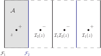
Figure 2: If the annulus $\mathcal{A}$ is represented as $\mathcal{T}/(\mathbb{Z}_{2}\times\mathbb{Z}_{2})$, the bosonic propagator for ND boundary conditions can be obtained by using three mirror charges of varying signs.

One can easily check that this propagator satisfies Neumann conditions on $\mathcal{F}_{1}$ and Dirichlet conditions on $\mathcal{F}_{2}$. For the fermion propagator, we have to consider different spin structures given by the following relations:

$$\Psi^{i}(\mathcal{I}_{1}(z))=A_{1}\Psi^{i}(z);\qquad\Psi^{i}(\mathcal{I}_{2}(z))=-A_{2}\Psi^{i}(z);\qquad\Psi^{i}(\mathcal{J}(z))=A_{3}\Psi^{i}(z).$$ (34)

where $\mathcal{J}$ is the translation $z\rightarrow z+\tau$. As explained in section 2.2, $A_{1}$ and $A_{2}$ must be chosen from $\pm\tau_{1}$. Also, their overall sign can be fixed. On the other hand, $\mathcal{J}$ induces an orientation-preserving loop, implying $A_{3}\in\{\pm\mathbf{1},\pm\tau_{3}\}$. Consistency requires $A_{3}$ to commute with both $A_{1}$ and $A_{2}$ so that altogether we find:

$$A_{1}=\tau_{1};\qquad A_{2}=\pm\tau_{1};\qquad A_{3}=\pm\mathbf{1}.$$ (35)

The different signs in this equation represent four different spin structures. We find the fermion propagator by starting with a torus $\mathcal{T}^{(2,2)}$ and using the method of images:

$$\langle\Psi^{i}(z,\overline{z})(\Psi^{i})^{tr}(w,\overline{w})\rangle_{ND}=G^{ii}\Big{\{}s_{2,2}(z,w)+A_{1}s_{2,2}(-\overline{z},w)-A_{2}s_{2,2}(1-\overline{z},w)\\ -A_{1}A_{2}s_{2,2}(1+z,w)+A_{3}s_{2,2}(\tau+z,w)+A_{1}A_{3}s_{2,2}(\tau-\overline{z},w)\\ -A_{2}A_{3}s_{2,2}(1+\tau-\overline{z},w)-A_{1}A_{2}A_{3}s_{2,2}(1+\tau+z,w)\Big{\}}$$ (36)

where $s$ is defined in equation (14). The fermion propagator on the annulus with ND-boundary conditions was also given in the appendix of reference [19] in terms of Jacobi theta functions with characteristics.

Intersecting D-branes

Next, we consider two D-branes of the same dimension intersecting each other. This configuration leads to open string modes which are localized at the brane intersection. As a consequence, scattering amplitudes involving an annulus stretching from one brane to the other renormalize the effective action on the intersection locus. In the general case, strings stretching between two intersecting branes obey NN- and DD-boundary conditions in a number of directions. The remaining dimensions can be arranged in pairs, $\mathbf{X}^{i}=(X^{i},Y^{i})$, on which the two branes intersect at an angle $\theta_{i}$ respectively. We choose coordinates such that the first brane, $D_{1}$, is aligned along the $X^{i}$ axes. Then, the second brane, $D_{2}$, obeys $Y_{i}=\tan(\theta_{i})X^{i}$. For a given pair $\mathbf{X}$ of worldsheet fields, a non-vanishing angle mixes the correlators of its components. The propagator for $\mathbf{X}$, written in matrix notation, acquires off-diagonal elements. Guided by our approach in the previous paragraphs, we should define two different antiholomorphic involutions on a covering torus, split the worldsheet coordinates into parallel and perpendicular components with respect to the corresponding brane and (anti-)symmetrize the torus propagator appropriately. More concretely, for a given worldsheet involution $\mathcal{I}_{i}$, we define a spacetime action $R_{i}$ and combine the two maps into a pair $g_{i}\equiv(R_{i},\mathcal{I})$ which acts on worldsheet fields as

$$g_{i}:\mathbf{X}(z)\mapsto(R_{i}\mathbf{X})(\mathcal{I}_{i}^{-1}(z))$$ (37)

If we define the spacetime action to be

$$R_{1}=\tau_{3},\qquad\qquad R_{2}=R(\theta)\tau_{3}R(\theta)^{-1},$$ (38)

where $\tau_{3}$ is the third Pauli matrix and $R(\theta)$ is a rotation by $\theta$ in the $(X,Y)$-plane, then symmetrizing a torus propagator under $g_{i}$ leads to Dirichlet conditions with respect to $D_{i}$ on the respective fixed point locus of $f_{i}$. However, note that $R_{1}$ and $R_{2}$ generally do not commute and the set $\{\mathbf{1},R_{1},R_{2}\}$ does not close under matrix multiplication. In fact, $R_{1}$ and $R_{2}$ represent reflections about the respective branes and the product of two reflections is a rotation,

$$R_{2}R_{1}=R(2\theta).$$ (39)

Therefore, if the branes intersect at a rational angle, $\theta\in 2\pi\mathbb{Q}$, the group which is generated by $R_{1}$ and $R_{2}$ is finite. More precisely, if $\theta=\pi p/q$ with two relatively prime integers, $p<q$, the group $\langle R_{1},R_{2}\rangle$ is the dihedral group $D_{q}$ (see appendix A). In order for $g_{1}\circ g_{2}$ to define a group operation, $\mathcal{I}_{1}$ and $\mathcal{I}_{2}$ have to be in a representation of $D_{q}$ as well. We choose the following representation of $D_{q}$ on a covering torus $\mathcal{T}^{(q,1)}$ with complex structure $\tau=it/2$:

$$\mathcal{I}_{1}:z\mapsto-\overline{z};\qquad\qquad\mathcal{I}_{2}:z\mapsto 1-\overline{z}$$ (40)

Here, $\mathcal{I}_{2}\circ\mathcal{I}_{1}$ is a translation by $1$ and therefore $(\mathcal{I}_{2}\circ\mathcal{I}_{1})^{q}$ is the identity on $\mathcal{T}^{(q,1)}$. Finally, we obtain the propagator for one pair of worldsheet scalars:

$$\langle\mathbf{X}(z,\overline{z})\mathbf{X}^{tr}(w,\overline{w})\rangle =\sum_{h\in D_{q}}P_{q,1}(h^{-1}z,w)$$ (41)

$$=\sum_{n=0}^{q-1}R(2\theta n)\left(P_{q,1}(z-n,w)+\tau_{3}P_{q,1}(-\overline{z}+n,w)\right),$$ (42)

where $P_{q,1}$ is the boson propagator (11) in matrix notation. In order to derive this expression, we generate $D_{q}$ by a reflection and a rotation rather than by two different reflections. A fundamental domain for the annulus is given by $\mathcal{A}=[0,1/2]\times i[0,t/2]$, which exhibits the correct open string normalization. As a check, one can verify that our expression for the propagator satisfies the correct boundary conditions on $\partial\mathcal{A}$. The procedure for obtaining the fermion propagators is analogous to the case of D-branes of different dimensionality. We define the spin structure of the fermionic fields by

$$\mathbf{\Psi}(\mathcal{I}_{1}(z))=R_{1}A_{1}\mathbf{\Psi}(z);\qquad\mathbf{\Psi}(\mathcal{I}_{2}(z))=R_{2}A_{2}\mathbf{\Psi}(z);\qquad\mathbf{\Psi}(\mathcal{J}(z))=A_{3}\mathbf{\Psi(z)}.$$ (43)

where $\mathcal{J}$ is the translation $z\rightarrow z+\tau$, the $R_{i}$ act on spacetime indices and the $A_{i}$ act on spinor indices. Consistency requires:

$$A_{1}=\tau_{1};\qquad A_{2}=\xi\tau_{1};\qquad A_{3}=\pm\mathbf{1},$$ (44)

with $\xi=\pm 1$. Using equation (39), it follows that $\mathbf{\Psi}(z+q)=\xi^{q}\mathbf{\Psi}(z)$ and therefore, in order to ensure periodicity on the covering torus, we need $q$ to be even. If this is not the case from the beginning, we simply drop the condition that $p$ and $q$ in $\theta=p/q$ be relatively prime, allowing us to choose $q$ even. Then, the holonomy group for the bosonic fields will only be a subgroup of $D_{q}$ but expression (41) remains unchanged. The fermion propagator reads:

$$\langle\mathbf{\Psi}(z,\overline{z})\mathbf{\Psi}^{tr}(w,\overline{w})\rangle=\sum_{k=0}^{q-1}\xi^{k}\Big{\{}R(2\theta k)S_{q,2}(z-k,w)+(R(2\theta k)\tau_{3})A_{1}S_{q,2}(-\overline{z}+k,w)\\ +R(2\theta k)A_{3}S_{q,2}(z-k+\tau,w)+(R(2\theta k)\tau_{3})A_{3}A_{1}S_{q,2}(-\overline{z}+k+\tau,w)\Big{\}}$$ (45)

where $S_{q,2}$ is the fermion propagator (13) in matrix form and it is understood that $R(2\theta k)$ acts on spacetime indices (as well as factors of $\tau_{3}$ grouped together with it) whereas the $A_{i}$ act on spinor indices.

Twisted annuli

For a twisted annulus, the bosonic fields do not return to themselves upon going around the closed cycle once but only up to a transformation $g\in G$ where $G$ is the subgroup of the orientifold group which contains all pure spacetime transformations. The path integral on the twisted annulus vanishes unless both boundaries lie on D-branes which are invariant under $g$. To see this, consider the loop channel picture where an open string stretching from one D-brane to another is projected onto itself after propagating for a time $t$ and being subjected to the twist.

For any supersymmetry-preserving orientifold, $G$ has to be a subgroup of $SO(6)$. This means that any given element $g\in G$ can be written as a product of three independent rotations acting on mutually orthogonal two-dimensional coordinate planes (cf. the discussion following equation (23)). Hence, we may define pairs of coordinates $\mathbf{X}^{i}=(X^{i},Y^{i})$ such that $g$ acts on these through rotations by an angle $\theta^{(i)}$ respectively. If $G$ is Abelian, we may choose the same coordinate frame for all possible twists $g$. Otherwise, we have to take different coordinate frames for different twists. For a given coordinate pair $\mathbf{X}$, a D-brane can be either spacetime-filling, point-like or a straight line. The spacetime-filling and point-like configurations are invariant under rotations. Combining these leads to boundary conditions of the NN-, DD- or ND-type. The construction of propagators on twisted annuli with the respective boundary conditions is fairly obvious and proceeds along the lines of the twisted torus construction. Here, we only give the results. For the boson propagator on a twisted annulus with doubly NN- or DD- boundary conditions, choose an integer $N$ such that $g$ acts on $\mathbf{X}$ through a rotation by an angle $\theta=2\pi/N$. Then, using the method of images, one finds

$$\langle\mathbf{X}(z,\overline{z})\mathbf{X}^{tr}(w,\overline{w})\rangle_{\theta,NN/DD}=\sum_{n=0}^{N-1}R(n\theta)\left(P_{1,N}(z-n\tau,w)\pm P_{1,N}(-\overline{z}-n\tau,w)\right)$$ (46)

Here, $P_{1,N}$ is the boson propagator (11) in matrix form and $R(\theta)$ is a rotation by an angle $\theta$. The plus and minus sign apply to NN- and DD-boundary conditions respectively. The fermion fields can be smoothly continued to periodic fields on a covering torus $\mathcal{T}^{2,2N}$. The spin structure on the twisted annulus is defined by

$$\mathbf{\Psi}(-\overline{z})=\pm\tau_{1}\mathbf{\Psi}(z),\qquad\mathbf{\Psi}(1-\overline{z})=\pm\xi_{1}\tau_{1}\mathbf{\Psi}(z),\qquad\mathbf{\Psi}(z+\tau)=\xi_{2}R(\theta)\mathbf{\Psi}(z)$$ (47)

where $\mathbf{\Psi}$ is the fermion spacetime doublet corresponding to the bosonic coordinate $\mathbf{X}$ and it is understood that $R(\theta)$ acts on spacetime indices. Again, the plus and minus signs apply to NN- and DD-boundary conditions respectively. The spin structure is parameterized by the numbers $\xi_{1}$ and $\xi_{2}$ each of which can be either plus or minus one. Then, the fermion propagator is given by:

$$\langle\mathbf{\Psi}(z,\overline{z})\mathbf{\Psi}^{tr}(w,\overline{w})\rangle_{\theta,NN/DD}=\sum_{n=0}^{2N}\xi_{1}^{n}R(n\theta)\Big{(}AS_{2,2N}(z-n\tau,w)\pm\tau_{3}S_{2,2N}(-\overline{z}-n\tau,w)\\ \pm\xi_{2}\tau_{3}S_{2,2N}(1-\overline{z}-n\tau,w)+\xi_{2}S_{2,2N}(z+1+n\tau,w)\Big{)}$$ (48)

where $S_{2,2N}$ is the fermion propagator (13) in matrix form. The propagator (48) can also be obtained by introducing a single mirror charge on a twisted torus. This technique was used in reference [19] to obtain the fermion propagator in terms of Jacobi theta functions with characteristics. The boson propagator on the twisted annulus with doubly ND-boundary conditions is given by

$$\langle\mathbf{X}(z,\overline{z})\mathbf{X}^{tr}(w,\overline{w})\rangle_{\theta,ND}=\sum_{n=0}^{N-1}R(n\theta)\Big{(}P_{1,N}(z-n\tau,w)+P_{1,N}(-\overline{z}-n\tau,w)\\ -P_{1,N}(1-\overline{z}-n\tau,w)-P_{1,N}(z+1-n\tau,w)\Big{)}.$$ (49)

The spin structure on the twisted ND-annulus is defined by

$$\mathbf{\Psi}(-\overline{z})=\tau_{1}\mathbf{\Psi}(z),\qquad\mathbf{\Psi}(1-\overline{z})=-\xi_{1}\tau_{1}\mathbf{\Psi}(z),\qquad\mathbf{\Psi}(z+\tau)=\xi_{2}R(\theta)\mathbf{\Psi}(z)$$ (50)

and the fermion propagator is given by

$$\langle\mathbf{\Psi}(z,\overline{z})\mathbf{\Psi}^{tr}(w,\overline{w})\rangle_{\theta,ND}=\sum_{n=0}^{2N}\xi_{1}^{n}R(n\theta)\Big{(}AS_{2,2N}(z-n\tau,w)+\tau_{3}S_{2,2N}(-\overline{z}-n\tau,w)\\ -\xi_{2}\tau_{3}S_{2,2N}(1-\overline{z}-n\tau,w)-\xi_{2}S_{2,2N}(z+1+n\tau,w)\Big{)}.$$ (51)

Finally, we consider boundary conditions corresponding to a pair of D-branes intersecting on the $\mathbf{X}$-plane at an angle $\phi$. As explained above, the only possible twist in this case is a rotation by $\pi$, i.e. a $\mathbb{Z}_{2}$ twist $g:\mathbf{X}\rightarrow-\mathbf{X}$. Then, if we choose coordinates such that the first D-brane is aligned with the X-axis, the boson propagator is given by

$$\langle\mathbf{X}(z,\overline{z})\mathbf{X}^{tr}(w,\overline{w})\rangle=\sum_{n=0}^{q-1}R(2\theta n)\Big{(}P_{q,2}(z-n,w)+\tau_{3}P_{q,2}(-\overline{z}+n,w)\\ -P_{q,2}(z-n+\tau,w)-\tau_{3}P_{q,2}(-\overline{z}+n+\tau,w)\Big{)},$$ (52)

where $q$ is an integer such that $q\phi$ is a multiple of $2\pi$. The spin structure and fermion propagator are given by equations (44) and (45) respectively with the substitution $A_{3}\rightarrow-A_{3}$.

3.4 The Möbius strip

The Möbius strip describes interactions between a D-brane and an O-plane. The fundamental group of the Möbius strip is generated by one cross-cap loop. We choose coordinates such that the twist associated to the loop can be described as a product of independent rotations of some coordinate planes $\mathbf{X}^{i}\equiv(X^{i},Y^{i})$ by an angle $\theta_{i}$ respectively. If for a given coordinate plane, the D-brane we are concerned with is neither plane-filling nor point-like, we can rotate the coordinates such that the brane becomes fully aligned with the X-axis. Thus, we have to distinguish three cases, corresponding to (N,N)-, (D,D)- and (N,D)-boundary conditions along the (X,Y)-axes respectively.

(N,N) boundary conditions

For a plane-filling D-brane, we obtain the propagator by a simple generalization of method described in references [14, 16]. We start with a skew torus $\mathcal{T}^{(1,q)}$, where $q\theta=0\mod 2\pi$, with a complex structure parameter $\tau=1/2+it/2$. Then, identifying points under the involution $\mathcal{I}:z\mapsto-\overline{z}$ and the translation $\mathcal{J}:z\mapsto z+\tau$ introduces a boundary and a cross-cap. Note that $\mathcal{I}$ and $\mathcal{J}$ commute up to a $\mathcal{T}^{(1,q)}$-lattice translation. Symmetrizing the torus propagator under $\mathcal{I}$ leads to Neumann boundary conditions. On the other hand, symmetrizing under $\mathcal{J}$ with an associated spacetime action corresponding to a rotation by $\theta$ leads to the correct loop periodicity. Thus, the bosonic propagator reads:

$$\langle\mathbf{X}(z,\overline{z})\mathbf{X}^{tr}(w,\overline{w})\rangle^{(N,N)}_{\theta}=\sum_{n=0}^{q-1}R(n\theta)\big{(}P_{1,q}(z-\tau n,w)+P_{1,q}(-\overline{z}-\tau n,w)\big{)}$$ (53)

We can choose $\mathcal{M}=[0,1/2]\times i[0,t/2]$ as the fundamental regime for the Möbius strip. This result can be regarded as a symmetrization under $\mathbb{Z}_{2}\times\mathbb{Z}_{q}$ where the $\mathbb{Z}_{2}$- ‘reflection’ is represented trivially on space-time. The spin structure of the Möbius strip is defined by

$$\mathbf{\Psi}(\mathcal{I}z)=A_{1}\mathbf{\Psi}(z);\qquad\mathbf{\Psi}(\mathcal{J}z)=R(\theta)A_{2}\mathbf{\Psi}(z)$$ (54)

where $R(\theta)$ acts on the spacetime indices and $A_{1}=\tau_{1}$ as well as $A_{2}\in\{\pm\mathbf{1},\pm\tau_{3}\}$ act on spinor indices. The fermion propagator reads:

$$\langle\mathbf{\Psi}(z,\overline{z})\mathbf{\Psi}^{tr}(w,\overline{w})\rangle^{(N,N)}_{\theta}=\sum_{n=0}^{2q-1}R(n\theta)A_{2}^{n}\big{(}S_{2,2q}(z-\tau n,w)+A_{1}S_{2,2q}(-\overline{z}-\tau n,w)\big{)}$$ (55)

(D,D) boundary conditions

The case of a point-like brane is very similar. One simply has to anti-symmetrize under $\mathcal{I}$ to obtain Dirichlet boundary conditions. Note that in order to retain the correct loop periodicity, one has to assign a spacetime action $\mathbf{X}\mapsto-R(\theta)\mathbf{X}$ to the translation $\mathcal{J}$. The bosonic propagator reads:

$$\langle\mathbf{X}(z,\overline{z})\mathbf{X}^{tr}(w,\overline{w})\rangle^{D,D}_{\theta}=\sum_{n=0}^{2q-1}(-1)^{n}R(n\theta)\big{(}P_{1,2q}(z-\tau n,w)-P_{1,2q}(-\overline{z}-\tau n,w)\big{)}$$ (56)

Here, we use a covering torus $\mathcal{T}^{(1,2q)}$ in order to include the case where $2\pi/\theta$ is odd. For even $2\pi/\theta$, there is a redundancy in the above expression. Again, we symmetrize under $\mathbb{Z}_{2}\times\mathbb{Z}_{q}$ where the $\mathbb{Z}_{2}$ is represented as $\mathbf{X}\mapsto-\mathbf{X}$ on spacetime. The spin structure is defined by

$$\mathbf{\Psi}(\mathcal{I}z)=A_{1}\mathbf{\Psi}(z);\qquad\mathbf{\Psi}(\mathcal{J}z)=-R(\theta)A_{2}\mathbf{\Psi}(z)$$ (57)

with $A_{1}=\tau_{1}$ and $A_{2}\in\{\pm\mathbf{1},\pm\tau_{3}\}$. The fermion propagator reads:

$$\langle\mathbf{\Psi}(z,\overline{z})\mathbf{\Psi}^{tr}(w,\overline{w})\rangle^{(N,N)}_{\theta}=\sum_{n=0}^{2q-1}(-1)^{n}R(n\theta)A_{2}^{n}\big{(}S_{2,2q}(z-\tau n,w)-A_{1}S_{2,2q}(-\overline{z}-\tau n,w)\big{)}$$ (58)

(N,D) boundary conditions

Symmetrizing the torus propagator under $\mathcal{I}$ combined with a space-time reflection about the $X$-axis leads to the correct boundary conditions. Then, in order to obtain the correct loop periodicity, one has to combine $\mathcal{J}$ with a rotation by $\theta$, followed by a reflection about the $X$-axis. This means that we have to symmetrize under $D_{q}$. The result is:

$$\langle\mathbf{X}(z,\overline{z})\mathbf{X}^{tr}(w,\overline{w})\rangle^{N,D}_{\theta}=\sum_{n=0}^{2q-1}\left(\tau_{3}R(\theta)\right)^{n}\big{(}P_{1,2q}(z-\tau n,w)+\tau_{3}P_{1,2q}(-\overline{z}-\tau n,w)\big{)}$$ (59)

Using $\tau_{3}R(\theta)=R(-\theta)\tau_{3}$, it is easy to check that the propagator exhibits the correct periodicity. The spin structure is defined by

$$\mathbf{\Psi}(\mathcal{I}z)=A_{1}\mathbf{\Psi}(z);\qquad\mathbf{\Psi}(\mathcal{J}z)=(\tau_{3}R(\theta))A_{2}\mathbf{\Psi}(z)$$ (60)

with $A_{1}=\tau_{1}$ and $A_{2}\in\{\pm\mathbf{1},\pm\tau_{3}\}$. The fermion propagator reads:

$$\langle\mathbf{\Psi}(z,\overline{z})\mathbf{\Psi}^{tr}(w,\overline{w})\rangle^{(N,N)}_{\theta}=\sum_{n=0}^{2q-1}(\tau_{3}^{n}R(n\theta))A_{2}^{n}\big{(}S_{2,2q}(z-\tau n,w)+\tau_{3}A_{1}S_{2,2q}(-\overline{z}-\tau n,w)\big{)}$$ (61)

In this expression, $\tau_{3}$ acts on spacetime indices.

4 Discussion and outlook

In this paper, we have obtained the propagators of the superstring worldsheet fields on one-loop surfaces for non-trivial holonomy and boundary conditions. Using our results, it is possible to compute one-loop corrections to scattering amplitudes in orientifolds of the type II string theories, including cases where D-branes of different dimensions or D-branes intersecting at angles are present. Although our results can be used most directly in computing scattering amplitudes involving NS-NS states only, they also apply to interactions with the R-NS and R-R sector. We will briefly comment on the computation of spin field correlation functions further down.

From the results for scattering amplitudes, one can obtain the effective action for the background in question using the S-matrix approach. Orientifolds with coincident stacks of D-branes and orientifolds with intersecting D-branes constitute a large class of perturbatively consistent string theory vacua. Furthermore, a great number of phenomenologically attractive orientifold models have been constructed which come quite close to having realistic low-energy behaviour. Orientifold models are seriously constrained by consistency conditions imposed by tadpole cancellation. The only known models with full tadpole cancellation are supersymmetric orientifolds. While the superpotential is protected from perturbative corrections by supersymmetry, the Kähler potential does receive corrections at one-loop. The latter might be interesting in terms of moduli stabilization. For instance, one-loop corrections might lead to a non-trivial dependence of the Kähler potential on the overall size of the extra dimensions and to a non-trivial scalar potential for the corresponding Kähler modulus. One-loop corrections might also help to stabilize the string coupling at small values. This prospect would offer a detailed view on the string theory landscape in a particular exactly calculable region.

As a step in this direction, we propose to expand on the computation of the induced Einstein-Hilbert term for intersecting D-branes [21] or D-branes at orbifold singularities [22] (see also references [23, 24, 25, 26]). The respective computations involve two-graviton scattering on one-loop surfaces with the gravitons polarized along the non-compact directions. The computation of metric moduli interaction terms would be similar in form but with polarizations transverse to the non-compact directions and thereby requiring propagators of the form we derived in this paper.

A complete characterization of the low-energy effective action requires knowledge of R-R and R-NS scattering amplitudes. Here, we briefly point out how these can be computed using the methods developed in this paper. Vertex operators in Ramond sectors are constructed using spin fields [27]. Unfortunately, this means that it is no longer possible to use Wick contractions in order to directly reduce the computation of general scattering amplitudes to the computation of free field propagators. Instead, one needs the full n-point functions involving an arbitrary number of worldsheet fermions and spin fields. These can also be obtained using the method of images as developed in this paper. The spin fields are given by $S(z)=C_{\lambda}e^{i\lambda_{i}\phi_{i}}$ where $\lambda$ is a polarization spinor and $\phi_{i}$ are the bosonized worldsheet fermions, $e^{i\phi_{i}}\cong 2^{-1/2}(\psi^{2i}+i\psi^{2i+1})$. $C$ is a cocycle which imposes the correct anticommutation relations. The holonomy and boundary conditions for the fermion fields $\psi^{\mu}$ and $\tilde{\psi}^{\mu}$ can be translated to conditions for their bosonizations $\phi_{i}$ and $\tilde{\phi}_{i}$. These can be rewritten as invariance of the boson doublet $\Phi_{i}\equiv(\phi_{i},\tilde{\phi}_{i})$ under the (generalized) holonomy group $\tilde{G}$, i.e. $\tilde{g}\Phi=\Phi$ where the action of $\tilde{g}$ is determined by the corresponding fermion transformation (5). Although in general the action of $\tilde{G}$ on $\Phi$ will be given by highly non-trivial relations, it can easily be obtained in the special case where the spacetime action of $\tilde{G}$ independently rotates pairs of coordinates: spacetime rotations are replaced by shifts of the bosonized fields. Having derived the action of $\tilde{G}$ on $\Phi$, one can proceed along the lines of section 3 and compute any fermion n-point function on a one-loop surface $\sigma$ by reconstructing the worldsheet from a covering torus as $\sigma=\mathcal{T}/\tilde{G}$ and symmetrizing the propagators for the bosonized fields under the action of $\tilde{G}$. Using this method, the spin field correlators can be derived from the correlators on the untwisted torus which can be found in reference [28].

A complete characterization of the low-energy effective action would also involve computing scattering amplitudes with twisted closed strings and open strings either obeying ND-boundary conditions or stretching from one brane to another brane which intersects the first brane at an angle. In all three cases, vertex operators have been constructed using twist fields. Scattering amplitudes involving twist fields at tree-level have been computed for twisted closed strings [29], for open ND-strings [30] and intersecting branes [31, 32, 33]. The corresponding methods would have to be appropriately extended and generalized.

Appendix A Dihedral Groups

The $q$-th Dihedral Group, $D_{q}$, is a non-Abelian permutation group of order 2q. It is the symmetry group of a regular q-sided polygon, consisting of reflections and rotations. The $q$-th Dihedral Group can be defined abstractly by

Figure 3: The polyhedral group $D_{8}$. It can be generated by two reflections, $x$ and $y$, or by one reflection and a rotation, $\rho$.

$$D_{q}\equiv\langle x,y|x^{2}=y^{2}=(xy)^{q}=1\rangle.$$ (62)

In the geometrical picture, $x$ and $y$ can be taken to be reflections about neighbouring symmetry axes of the polygon. Alternatively, the Dihedral group can be presented in the following way:

$$D_{q}\equiv\langle x,\rho|x^{2}=\rho^{q}=1;x\rho x^{-1}=\rho^{-1}\rangle.$$ (63)

The latter version is related to the first one by setting $\rho=xy$. Geometrically, this means that the symmetry group of a regular q-sided polygon can also be generated by a reflection and a rotation. The subgroup $\mathbb{Z}_{q}=\langle\rho\rangle$ is normal in $D_{q}$ which can therefore be written as a semidirect product:

$$D_{q}\equiv\mathbb{Z}_{q}\rtimes\mathbb{Z}_{2}$$ (64)

In this paper we basically use two different ways for $D_{q}$ to operate on a torus. The simplest group action is the one where $D_{q}$ operates naturally on one of the circles (picture a polygon inscribed in the circle) and leaves the other circle invariant. This generically implies two different fixed point loci corresponding to reflections about symmetry axes which cut the polygon at its corners and the middle of its sides respectively. Thus, we achieve different boundary conditions for the two boundaries of an annulus. For special values of the torus’ complex structure, both boundaries are joined and we obtain a representation of the Möbius strip. Another useful representation of the group action is obtained by assigning an additional shift along half of the second circle to all reflections. This is compatible with the group structure and as a consequence of this modification, there are no fix-points under the group action. Therefore, the latter group action is useful in constructing propagators on the Möbius strip and Klein bottle worldsheet.

Appendix B Comparison to existing results.

Using the method of images, one can easily obtain expressions for the fermion propagators on an untwisted torus with non-trivial spin structure s (this was first suggested in [14]). For the left-moving mode, the propagators are given by

$$\langle\psi(z)\psi(w)\rangle_{s}=P^{F}_{2,2}(z,w)+a_{s}P^{F}_{2,2}(z+1,w)+b_{s}P^{F}_{2,2}(z+\tau,w)+a_{s}b_{s}P^{F}_{2,2}(z+1+\tau,w)$$ (65)

s	a	b	$\alpha$	$\beta$
1	1	1	0	0
2	1	-1	0	$\frac{1}{2}$
3	-1	-1	$\frac{1}{2}$	$\frac{1}{2}$
4	-1	1	$\frac{1}{2}$	0

Table 2: spin structure conventions

where $P^{F}$ is the fermion propagator (15) and the conventional relation of $(a,b)$ to the spin structure s is given in table 2. By construction, this expression has the right periodicity and pole structure if one constrains it to a fundamental domain of the torus $\mathcal{T}^{(1,1)}$. However, on first sight it seems to be different from the more familiar expression (see e.g. [16])

$$\langle\psi(z)\psi(w)\rangle_{s}=-\frac{1}{4}\frac{\vartheta_{s}(z-w|\tau)\vartheta_{1}^{\prime}(0|\tau)}{\vartheta_{s}(0|\tau)\vartheta_{1}(z-w|\tau)}$$ (66)

for fermion propagators on a torus with even spin structure ($s=2,3,4$). That the two different expressions are actually equal follows from the following argument: The propagators (65) and (66) are elliptic functions (i.e. meromorphic and doubly periodic) with periods $2$ and $2\tau$. Both propagators have four simple poles per fundamental cell. In both cases, the poles are at $z-w=0,1,\tau,1+\tau$ with residues $-1/4,-a_{s}/4,-b_{s}/4,-a_{s}b_{s}/4$ respectively, i.e. the infinite part of both expressions is identical. It follows that the difference of the two propagators is an analytic function on the whole complex plain which is bounded and therefore constant by Liouville’s theorem. By evaluating the two expressions at a particular point, one establishes that this constant vanishes and that the two expressions are equal.

A similar argument also holds for the twisted torus in Abelian orbifolds. Consider a pair of coordinates $\mathbf{X}=(X_{1},X_{2})$ and $\mathbf{\Psi}=(\Psi_{1},\Psi_{2})$ such that a given element $g_{i}$ of the orbifold group acts on these through rotations by an angle $\theta_{1}$. For the twisted torus, there are two independent closed loops along which the worldsheet fields return to themselves up to the action of group elements $\theta_{2}$ and $\theta_{2}$ respectively. Let us consider the fermionic fields first. For these, the periodicity conditions may include an additional sign change. Therefore, we are interested in fermionic fields $\mathbf{\Psi}(z)$ on the torus $\mathcal{T}=\mathbb{C}/(\mathbb{Z}\times\tau\mathbb{Z})$ with periodicity conditions

$$\mathbf{\Psi}(z+1)=A_{1}R(\theta_{1})\mathbf{\Psi}(z),\qquad\mathbf{\Psi}(z+\tau)=A_{2}R(\theta_{2})\mathbf{\Psi}(z),$$ (67)

Here, the $A_{i}\in\{1,\tau_{3}\}$ act on the spinor indices of $\mathbf{\Psi}$ whereas $R(\theta)$ denotes a spacetime rotation by an angle $\theta$. Then, as discussed in section 3.1, if we choose even integers $N$ and $M$ such that $N\theta_{1}$ and $M\theta_{2}$ are integer multiples of $2\pi$, the fermion propagator takes the following form:

$$\langle\mathbf{\Psi}(z,\overline{z})\mathbf{\Psi}^{tr}(w,\overline{w})\rangle_{\theta_{1},\theta_{2},(s,\tilde{s})}=\sum_{n=0}^{N-1}\sum_{m=0}^{M-1}R(n\theta_{1}+m\theta_{2})A_{1}^{n}A_{2}^{m}S_{N,M}(z-n-m\tau,w),$$ (68)

where $(s,\tilde{s})$ denotes the choice of spin structure (67) and $S_{N,M}$ is the fermion propagator (13). In order to compare this expression to the fermion propagator in reference [19], we go to the component notation for the fermionic fields. Let

$$\psi(z)=\frac{1}{\sqrt{2}}\left(\psi^{1}(z)+i\psi^{2}(z)\right),\qquad\overline{\psi}(z)=\frac{1}{\sqrt{2}}\left(\psi^{1}(z)-i\psi^{2}(z)\right)$$ (69)

be the complexified left-handed part of the fermionic coordinates. Furthermore, define $a=(A_{1})_{11}$ and $b=(A_{2})_{11}$. In terms of these, the periodicity conditions (67) for the left-handed fermion fields take the following form:

$$\psi(z+1) =ae^{i\theta_{1}}\psi(z),\qquad\overline{\psi}(z+1)=ae^{-i\theta_{1}}\overline{\psi}(z)$$ (70)

$$\psi(z+\tau) =be^{i\theta_{2}}\psi(z),\qquad\overline{\psi}(z+\tau)=be^{-i\theta_{2}}\overline{\psi}(z)$$ (71)

and likewise for the right-handed components. Then, if the pair of directions $(X_{1},X_{2})$ form a square torus, i.e. if for $i,j\in\{1,2\}$ we have a target space metric $G_{ij}=\eta_{ij}$ (after an appropriate renormalization), the fermion propagators (23) take the following form in complex notation:

$$\langle\psi(z)\overline{\psi}(w)\rangle_{\theta_{1},\theta_{2},s}=\sum_{n=0}^{N-1}\sum_{m=0}^{M-1}e^{in\theta_{1}+im\theta_{2}}a^{n}b^{m}P^{F}_{N,M}(z-n-m\tau,w)$$ (72)

All other correlators vanish. By construction, the fermion propagator, if viewed as a function on the unit torus, has a single pole at $z=w$ with a residue of $-\frac{1}{4}$. Furthermore, it picks up a phase $ae^{i\theta_{1}}$ under $z\rightarrow z+1$ and a phase $be^{i\theta_{1}}$ under $z\rightarrow z+\tau$. The same is true for the expression

$$-\frac{1}{4}\frac{\vartheta[^{\alpha+v_{1}}_{\beta+v_{2}}](z-w|\tau)\vartheta_{1}^{\prime}(0|\tau)}{\vartheta[^{\alpha+v_{1}}_{\beta+v_{2}}](0|\tau)\vartheta_{1}(z-w|\tau)}$$ (73)

involving Jacobi’s theta functions with characteristics. Here, $\alpha$ and $\beta$ can be read off table 2 and we define $v_{i}\equiv\theta_{i}/2\pi$. The same expression, in a different normalization, was used in reference [19], with $v_{1}=0$. Equality between expressions (72) and (73) can be established using an argument equivalent to the one given above for fermion propagators on an untwisted torus with even spin-structure. Starting with the expression (73) with $v_{1}=0$, it is straightforward to derive expressions for the twisted annulus and Möbius strip using the simple method of images as described in the appendix of reference [16]. The resulting expressions were used to compute various matter field couplings [19] and the masses of anomalous $U(1)$ gauge bosons [20] in four-dimensional orientifold vacua. It is also possible to obtain, in this way, the propagators for a Klein bottle which is twisted only in one direction. However, the same approach is unable to produce results for the most general Klein bottle, i.e. the Klein bottle with two independent twists.

References

- [1] D. Lust, Intersecting brane worlds: A path to the standard model?, Class. Quant. Grav. 21 (2004) S1399–1424 [hep-th/0401156].
- [2] E. Kiritsis, D-branes in standard model building, gravity and cosmology, Fortsch. Phys. 52 (2004) 200–263 [hep-th/0310001].
- [3] J. H. Schwarz, Superstring theory, Phys. Rept. 89 (1982) 223–322.
- [4] S. B. Giddings, S. Kachru and J. Polchinski, Hierarchies from fluxes in string compactifications, Phys. Rev. D66 (2002) 106006 [hep-th/0105097].
- [5] S. Kachru, R. Kallosh, A. Linde and S. P. Trivedi, De sitter vacua in string theory, Phys. Rev. D68 (2003) 046005 [hep-th/0301240].
- [6] M. Berg, M. Haack and B. Kors, Loop corrections to volume moduli and inflation in string theory, hep-th/0404087.
- [7] A. Sagnotti, Open strings and their symmetry groups, hep-th/0208020.
- [8] G. Pradisi and A. Sagnotti, Open string orbifolds, Phys. Lett. B216 (1989) 59.
- [9] N. Ishibashi and T. Onogi, Open string model building, Nucl. Phys. B318 (1989) 239.
- [10] P. Horava, Strings on world sheet orbifolds, Nucl. Phys. B327 (1989) 461.
- [11] M. Bianchi and A. Sagnotti, Twist symmetry and open string wilson lines, Nucl. Phys. B361 (1991) 519–538.
- [12] M. Bianchi and A. Sagnotti, On the systematics of open string theories, Phys. Lett. B247 (1990) 517–524.
- [13] E. G. Gimon and J. Polchinski, Consistency conditions for orientifolds and d-manifolds, Phys. Rev. D54 (1996) 1667–1676 [hep-th/9601038].
- [14] C. P. Burgess and T. R. Morris, Open and unoriented strings a la polyakov, Nucl. Phys. B291 (1987) 256.
- [15] N. Ohta, Cancellation of dilaton tadpoles and two loop finiteness in so(32) type i superstring, Phys. Rev. Lett. 59 (1987) 176.
- [16] I. Antoniadis, C. Bachas, C. Fabre, H. Partouche and T. R. Taylor, Aspects of type i - type ii - heterotic triality in four dimensions, Nucl. Phys. B489 (1997) 160–178 [hep-th/9608012].
- [17] C. Angelantonj and A. Sagnotti, Open strings, Phys. Rept. 371 (2002) 1–150 [hep-th/0204089].
- [18] M. Blau and L. Dabrowski, Spin structures on manifolds quotiented by discrete groups, . SISSA-116/87/FM.
- [19] P. Bain and M. Berg, Effective action of matter fields in four-dimensional string orientifolds, hep-th/0003185.
- [20] I. Antoniadis, E. Kiritsis and J. Rizos, Anomalous u(1)s in type i superstring vacua, Nucl. Phys. B637 (2002) 92–118 [hep-th/0204153].
- [21] T. J. Epple, Friedel, Induced gravity on intersecting branes, hep-th/0408105.
- [22] E. Kohlprath, Induced gravity in z(n) orientifold models, hep-th/0311251.
- [23] E. Kiritsis, N. Tetradis and T. N. Tomaras, Thick branes and 4d gravity, JHEP 08 (2001) 012 [hep-th/0106050].
- [24] I. Antoniadis, S. Ferrara, R. Minasian and K. S. Narain, R**4 couplings in m- and type ii theories on calabi-yau spaces, Nucl. Phys. B507 (1997) 571–588 [hep-th/9707013].
- [25] I. Antoniadis, R. Minasian and P. Vanhove, Non-compact calabi-yau manifolds and localized gravity, Nucl. Phys. B648 (2003) 69–93 [hep-th/0209030].
- [26] I. Antoniadis, R. Minasian, S. Theisen and P. Vanhove, String loop corrections to the universal hypermultiplet, Class. Quant. Grav. 20 (2003) 5079–5102 [hep-th/0307268].
- [27] D. Friedan, E. J. Martinec and S. H. Shenker, Conformal invariance, supersymmetry and string theory, Nucl. Phys. B271 (1986) 93.
- [28] J. J. Atick and A. Sen, Correlation functions of spin operators on a torus, Nucl. Phys. B286 (1987) 189.
- [29] L. J. Dixon, D. Friedan, E. J. Martinec and S. H. Shenker, The conformal field theory of orbifolds, Nucl. Phys. B282 (1987) 13–73.
- [30] J. Frohlich, O. Grandjean, A. Recknagel and V. Schomerus, Fundamental strings in dp-dq brane systems, Nucl. Phys. B583 (2000) 381–410 [hep-th/9912079].
- [31] M. Cvetic and I. Papadimitriou, Conformal field theory couplings for intersecting d-branes on orientifolds, Phys. Rev. D68 (2003) 046001 [hep-th/0303083].
- [32] S. A. Abel and A. W. Owen, Interactions in intersecting brane models, Nucl. Phys. B663 (2003) 197–214 [hep-th/0303124].
- [33] S. A. Abel and A. W. Owen, N-point amplitudes in intersecting brane models, Nucl. Phys. B682 (2004) 183–216 [hep-th/0310257].