Quantum $QED$ Flux Tubes in $2+1$ and $3+1$ Dimensions

N. Graham^a, V. Khemani^b,c, M. Quandt^d, O. Schröder^b, H. Weigel^e

Abstract

We compute energies and energy densities of static electromagnetic flux tubes in three and four spacetime dimensions. Our calculation uses scattering data from the potential induced by the flux tube and imposes standard perturbative renormalization conditions. The calculation is exact to one-loop order, with no additional approximation adopted. We embed the flux tube in a configuration with zero total flux so that we can fully apply standard results from scattering theory. We find that upon choosing the same on-shell renormalization conditions, the functional dependence of the energy and energy density on the parameters of the flux tube is very similar for three and four spacetime dimensions. We compare our exact results to those obtained from the derivative and perturbation expansion approximations, and find good agreement for appropriate parameters of the flux tube. This remedies some puzzles in the prior literature.

Keywords:  flux tubes, vacuum polarization energy, renormalization, derivative expansion

PACS:  11.10.Gh, 11.15.Kc, 11.27.+d, 12.20.Ds.

1 Introduction

Flux tubes in QED coupled to fermions exhibit a number of interesting phenomena, such as the Aharonov-Bohm effect [1], its consequences for fermion scattering [2], parity anomalies [3], formation of a condensate [4], and exotic quantum numbers [5, 6, 7]. The same (non-perturbative) features of the theory that give rise to these unusual phenomena make it more difficult to analyze this system with standard techniques, especially in calculations that require renormalization. The analysis in ref. [8] and the world line formalism in ref. [9] have addressed some of these issues. Here we provide a comprehensive approach drawing on techniques from scattering theory to analyze the one-loop energy and charge of this system.

Our primary motivation for this analysis is to shed light on vortices in more complicated field theories, especially the Z-string in the standard electroweak theory [10]. The Z-string is a vortex configuration carrying magnetic flux in the field of the Z-gauge boson. If a network of such objects existed at the electroweak phase transition, then it would be one key ingredient in a viable mechanism for electroweak baryogenesis without a first-order phase transition. Since the classical Z-string is known to be unstable [11], this scenario would require stabilization via quantum effects [12], perhaps by trapping heavy quarks along the string. We also expect that by extending our results to the Abelian Higgs model, they could be applied to Abrikosov flux tubes in Type II superconductors [13] or supersymmetric Abelian Higgs models [14].

We compare the one-loop energies and energy densities of electromagnetic vortices in $D=2+1$ and $D=3+1$ spacetime dimensions. The classical calculation is of course the same in the two cases. The quantum corrections to the energy could possibly be very different [9] because of the different divergence structure. In $D=3+1$, the bare one-loop energy is divergent and only after we impose renormalization conditions do we get a finite result. In $D=2+1$, in contrast, the bare energy is finite. However, a comparison between the two dimensionalities is sensible only when we use the same renormalization conditions, which requires a finite counterterm in the $D=2+1$ case to keep the photon field normalization the same. Without this finite renormalization, the $D=2+1$ and $D=3+1$ energies are qualitatively different. But after proper renormalization, we find that both the energies and energy densities are closely related.

We also study this problem to get a handle on several technical issues associated with the computation of the one-loop energy of a flux tube. As described in Section 3.2, an efficient way to compute the energy is to use scattering data of fermions in the background of the flux tube. However, vortex configurations give long-range potentials, which do not satisfy standard conditions in scattering theory [15], which would guarantee the analytic properties of scattering data. This leads to subtleties that are discussed in Section 4. We show that these puzzles arise only because an isolated flux tube is unphysical, and once a region of return flux is included, the scattering problem is well-defined and the puzzles disappear. In the limit where the return flux is infinitely spread out, the energy density becomes entirely localized at the original flux tube.

The paper is organized as follows: In the following Section we describe the theory and introduce electromagnetic flux tubes. We outline the computation of their classical and renormalized one–loop vacuum polarization energies in Section 3. We describe puzzles in this calculation that arise from an isolated flux tube in Section 4 and explain how these puzzles can be resolved by appropriate embedding of the flux tube in Section 5. We present numerical results for the energies, energy densities and charge densities in Section 6. In Section 7 we summarize our results and provide an outlook on related studies. Three Appendices give the technical details needed for the computation of quantum contributions to the energy and charge densities.

2 The Theory

We consider QED in spacetime dimensions $D=2+1$ and $D=3+1$, with a four-component fermion field, $\psi$, in both cases. The Lagrangian density is

$$\mathcal{L}^{(D)}=-\frac{1}{4}F_{\mu\nu}F^{\mu\nu}+\bar{\psi}(i\partial\hskip-6.00006pt/+eA\hskip-6.00006pt/-m)\psi+\mathcal{L}^{(D)}_{\rm CT}\,,$$ (1)

where the indices $\mu$ and $\nu$ run from $0$ to $D-1$ and $\mathcal{L}^{(D)}_{\rm CT}$ is the counterterm Lagrangian in $D$ spacetime dimensions. In $D=3+1$, this Lagrangian describes electromagnetism with a single four-component fermion of mass $m$ and charge $e$. In $D=2+1$, we have parity-invariant electromagnetism with two flavors of two-component fermions of equal mass $m$ and charge $e$. We are interested in static magnetic flux tubes. These are localized, cylindrically symmetric magnetic fields (pointing in the $z$ direction in $D=3+1$), with a net flux $F$ through the $xy$-plane. In the radial gauge, flux tubes arise from vortex configurations of gauge fields:

$$A_{0}=0\,,\quad\vec{A}=\frac{F}{2\pi r}f(r)\hat{e}_{\varphi}\,,$$ (2)

where $r^{2}=x^{2}+y^{2}$ measures the planar distance from the center of the vortex. The radial function $f(r)$ goes from 0 to 1. In $D=2+1$ the magnetic field is the radial function

$$B(r)=\frac{F}{2\pi r}\frac{df(r)}{dr}\,,$$ (3)

while in $D=3+1$ it is the vector field $\vec{B\,}(\vec{r\,})=B(r)\hat{e}_{z}$. For small $r$, we must have $f(r)$ going to zero at least quadratically for $B(r)$ and $\vec{A}(\vec{r})$ to be non–singular.

We often find it convenient to specify the flux in units of $2\pi/e$ and define the dimensionless quantity

$$\mathcal{F}=\frac{e}{2\pi}F\,.$$ (4)

In most cases we will take the example of a Gaußian flux tube of width $w$,

$$f_{G}(r)=1-e^{-r^{2}/w^{2}}\hbox{\qquad so that\qquad}B_{\rm G}(r)=B_{\rm G}(0)e^{-r^{2}/w^{2}}\,,$$ (5)

whose flux is

$$F_{\rm G}=\pi w^{2}B_{\rm G}(0)\,.$$ (6)

3 The Energy

We would like to to compute the total energy $E^{(3)}$ for $D=2+1$ and the energy per unit length $E^{(4)}$ for $D=3+1$, to one-loop order. In general, we would have to evaluate the appropriate matrix element of the energy momentum tensor. However, as we review in Appendix B, for static configurations the total energy is simply given by the negative one-loop effective action per unit time. Since the theory is Abelian, the photons do not have self-interactions and the one-loop effective action is obtained by integrating out the fermion field. The photon fluctuations start contributing only at two loops and higher, which we ignore.

To one loop order, the total energy is the sum of the classical energy, $E_{\rm cl}$, and the fermion vacuum polarization energy, $E^{(D)}_{\rm vac}$,

$$E^{(D)}=E_{\rm cl}+E^{(D)}_{\rm vac}\,.$$ (7)

For both cases, $D=2+1$ and $D=3+1$, the classical contribution is

$$E_{\rm cl}=\frac{1}{2}\int d^{2}rB^{2}(\vec{r\,})\,.$$ (8)

We extract the renormalized fermion vacuum polarization energy from the one–loop effective action

$$E_{\rm vac}^{(3)} = \lim_{T\rightarrow\infty}\frac{i}{T}\left[\,\mbox{ln}\,\mbox{Det}(i\partial\hskip-6.00006pt/+eA\hskip-6.00006pt/-m)-\,\mbox{ln}\,\mbox{Det}(i\partial\hskip-6.00006pt/-m)\right]+E^{(3)}_{\rm CT}\,,$$ (9)

$$E_{\rm vac}^{(4)} = \lim_{T,L_{z}\rightarrow\infty}\frac{i}{TL_{z}}\left[\,\mbox{ln}\,\mbox{Det}(i\partial\hskip-6.00006pt/+eA\hskip-6.00006pt/-m)-\,\mbox{ln}\,\mbox{Det}(i\partial\hskip-6.00006pt/-m)\right]+E^{(4)}_{\rm CT}\,,$$ (10)

by dividing out the arbitrarily long time interval in both cases, and the arbitrary length of the vortex in $D=3+1$ dimensions. Note that the energy is always defined relative to a background where the electromagnetic fields are zero everywhere.

3.1 Renormalization

The counterterms introduced in eq. (10) originate from the standard counterterm Lagrangian, ${\cal L}_{\rm ct}=-\frac{C^{(D)}}{4}F_{\mu\nu}^{2}$. Since we do not consider electric fields, the counterterms are quadratic in the magnetic field

$$E^{(D)}_{\rm CT}=\frac{C^{(D)}}{2}\,\int d^{2}xB^{2}\,.$$ (11)

To fix the counterterm coefficient, $C^{(D)}$, we choose on-shell renormalization conditions, which require that the residue at the $q^{2}=0$ pole of the photon propagator is unity to ensure that one-photon states remain normalized. We obtain

$$C^{(D)}=-\frac{4e^{2}}{3(4\pi)^{D/2}}\frac{\Gamma\left(2-\frac{D}{2}\right)}{m^{4-D}}\,$$ (12)

which becomes

$$C^{(3)}=-\frac{e^{2}}{6\pi m}\,,$$ (13)

in $D=2+1$ dimensions, and the dimensionally regularized quantity

$$C^{(4-\epsilon)}=-\frac{e^{2}}{12\pi^{2}}\left(\frac{2}{\epsilon}-\gamma+\,\mbox{ln}\,\frac{4\pi}{m^{2}}\right)\,.$$ (14)

for dimensions approaching $D=3+1$, where $\epsilon=4-D$.

The counterterm, ${\cal L}_{\rm ct}$ renormalizes the bare photon field and fermion charge,

$$A^{\mu}=(1+C^{(D)})^{-1/2}A_{\rm bare}^{\mu}\quad{\rm and}\quad e=(1+C^{(D)})^{1/2}e_{\rm bare}\,.$$ (15)

In the absence of photon fluctuations, the bare fermion field and mass do not get renormalized. In $D=3+1$ the counterterm is divergent and combines with the divergent functional determinant to give a finite, renormalized one-loop energy. In $D=2+1$, the counterterm is finite, but it still must be taken into account to ensure that the photon field remains canonically normalized. Since we want to compare the energies in $D=2+1$ and $D=3+1$, we must impose identical renormalization conditions in the two cases.

3.2 Functional Determinant

We use the phase shift approach [16, 17] to compute the functional determinant in eq. (10) exactly. The fermion vacuum energy is given by the renormalized sum over the shift in the zero-point energies of the fermion modes due to the presence of the background magnetic field. This calculation comprises a sum over bound state energies and an integral over the continuum energies weighted by the change in the density of states. These quantities are obtained from the Dirac equation for the fermion fields in the background of the flux tube. The explicit form of this equation is given in Appendix A, eqs. (51) and (54). Since the configuration that characterizes the flux tube is cylindrically symmetric, the fermion scattering matrix may be decomposed into partial waves labeled by the $z$-component of the total angular momentum, $M$. Then, in $D=2+1$, the change in the density of continuum states is given in terms of the phase shifts of the fermion scattering wave functions in the flux tube background,

$$\Delta\rho(k)=\sum_{M,\sigma}\frac{1}{\pi}\,\frac{d}{dk}\left[\delta_{M,\sigma}(k)\right]\,,$$ (16)

where $k$ is the magnitude of the momentum and $\sigma$ refers to all other discrete labels. For a given momentum $k$ there are two energy eigenvalues $\pm\sqrt{k^{2}+m^{2}}$ and two spin states. This four-channel scattering problem can easily be diagonalized, yielding four identical phase shifts (with the exception of the threshold at $k=0$, as discussed below). Therefore summing over the discrete labels merely gives a factor of four. We denote the result of this sum as $\delta_{M}(k)$. In $D=3+1$, we must also integrate over momenta in the $z$-direction [18]. The details of the phase shift calculation are given in Appendix A.

To renormalize the continuum integral, we subtract the first two terms in the Born expansion of the phase shift and add back in the corresponding energy in the form of the two-point Feynman diagram (a fermion loop with two insertions of the background potential). The details of this calculation are described in Appendices A and B. In $D=3+1$, the Born subtraction renders the integral over the continuum energies convergent. The ultraviolet divergences are isolated in the Feynman diagram, which when combined with the counterterm, eq. (11), gives the properly renormalized finite result. In $D=2+1$ the Born subtraction is finite, but implements the on-shell renormalization condition.

Our final expression for the renormalized fermion vacuum energy is the sum of the subtracted contribution of the bound and continuum modes, the Feynman diagram, and the counterterm:

$$E^{(D)}_{\rm vac}=E^{(D)}_{\delta}+E^{(D)}_{\rm FD}+E^{(D)}_{\rm CT}\,.$$ (17)

The contribution from the Born-subtracted mode sum can be expressed through scattering data,

$$E^{(3)}_{\delta} = \frac{1}{2}\sum_{j}\left(|\omega_{j}|-m\right)+\frac{1}{2\pi}\int_{0}^{\infty}dk\frac{k}{\sqrt{k^{2}+m^{2}}}\sum_{M}\bar{\delta}_{M}(k)\,,$$ (18)

$$E^{(4)}_{\delta} = -\frac{1}{8\pi}\sum_{j}\left(\omega_{j}^{2}\,\mbox{ln}\,\frac{\omega_{j}^{2}}{m^{2}}+m^{2}-\omega_{j}^{2}\right)-\frac{1}{4\pi^{2}}\int_{0}^{\infty}dkk\,\mbox{ln}\,\frac{k^{2}+m^{2}}{m^{2}}\sum_{M}\bar{\delta}_{M}(k)\,,$$ (19)

where $\omega_{j}$ are the energy eigenvalues of the discrete bound states. (Even though the configurations that we consider here do not have such bound states, we have included their contribution for completeness.) We have defined

$$\bar{\delta}_{M}(k)=\delta_{M}(k)-\delta_{M}^{(1)}(k)-\delta_{M}^{(2)}(k)\,,$$ (20)

where $\delta^{(i)}_{M}$ denotes the $i^{\rm th}$ term in the Born series expansion of the exact phase shift, $\delta_{M}$. Since we have subtracted the two leading contributions of the Born series, the remainder, $E^{(D)}_{\delta}$ comprises the sum of the third and higher order pieces.

Next we add back the two leading Born terms in form of Feynman diagrams. The first order diagram vanishes by Furry’s theorem. In dimensional regularization the unrenormalized second-order Feynman diagram energy is

$$E^{(D)}_{\rm FD}=\frac{8\pi\mathcal{F}^{2}}{(4\pi)^{D/2}}\int_{0}^{\infty}dp\left[\int_{0}^{\infty}dr\frac{df(r)}{dr}J_{0}(pr)\right]^{2}\int_{0}^{1}dx\frac{x(1-x)p\Gamma(2-D/2)}{[m^{2}+p^{2}x(1-x)]^{2-D/2}}\,.$$ (21)

Combining this expression with the counterterm energy, eq. (11), gives the renormalized Feynman diagram energy at the physical spacetime dimension. The result is to impose perturbative renormalization conditions on this non–perturbative calculation.

4 Subtleties of Configurations With Net Flux

We have described the general computation of the renormalized one-loop energies of magnetic flux tubes. Before proceeding with the calculation, however, we must address subtleties in the calculation of the phase shifts at zero momentum. These questions arise because the background potential does not satisfy standard asymptotic conditions in scattering theory. As is well-known from the Aharonov-Bohm effect, even if the magnetic fields are exponentially localized, the vector potential falls only as $1/r$, which is too slowly for many of the standard theorems of scattering theory to hold [15]. As a result, the phase shifts are discontinuous at threshold. Although this discontinuity does not cause problems for calculating the vacuum polarization energy, because the integrands in eqs. (18) and (19) remain smooth, we can no longer determine the number of bound states through Levinson’s theorem [19].

As described in Appendix A, we calculate the phase shifts in the background of a flux tube by deriving second-order differential equations from the Dirac equation. The asymptotic behavior as $r\to\infty$ of the coefficient functions in these differential equations is extracted from eqs. (56) in with $h(r)=\mathcal{F}$ and $\ell=M-\frac{1}{2}$,

$$g^{(1)^{\prime\prime}}_{\ell}(r)+\frac{g^{(1)^{\prime}}_{\ell}(r)}{r}+\left(k^{2}-\frac{(M-\frac{1}{2}-\mathcal{F})^{2}}{r^{2}}\right)g^{(1)}_{\ell}(r) = 0\,,$$

$$g^{(2)^{\prime\prime}}_{\ell}(r)+\frac{g^{(2)^{\prime}}_{\ell}(r)}{r}+\left(k^{2}-\frac{(M+\frac{1}{2}-\mathcal{F})^{2}}{r^{2}}\right)g^{(2)}_{\ell}(r) = 0\,,$$ (22)

where primes denote derivatives with respect to $r$. For large $r$ we do not have free Bessel differential equations whose index equals the angular momentum; rather the equations describe an ideal flux tube with profile function $f(r)\equiv 1$. If extended to the origin, such an ideal flux tube would generate a singular background potential.

Since the centrifugal barrier is shifted by the amount of the flux, the regular solutions to the asymptotic differential equations (22) are Bessel functions with a correspondingly shifted index,

$$g^{(1)}_{\ell}(r)=J_{|M-\frac{1}{2}-\mathcal{F}|}(kr)\quad{\rm and}\quad g^{(2)}_{\ell}(r)=J_{|M+\frac{1}{2}-\mathcal{F}|}(kr)\,.$$ (23)

From the asymptotic behavior of the Bessel functions, we read off a phase shift relative to the trivial configuration $A_{\mu}=0$ [20]

$$\Delta\delta_{M}(k)=\pi\left(|M-\frac{1}{2}|+|M+\frac{1}{2}|-|M-\frac{1}{2}-\mathcal{F}|-|M+\frac{1}{2}-\mathcal{F}|\right)\,,$$ (24)

where we have summed the phase shifts associated with the two radial functions, which corresponds to summing over the spin degrees of freedom. For a radially varying profile function $f(r)$ with $\lim_{r\to\infty}f(r)=1$, the second-order equations (56) allow us to compute phase shifts relative to the ideal flux tube, $\delta_{M,\rm ideal}$, to which $\Delta\delta_{M}$ must be added to obtain the phase shift relative to the trivial configuration:

$$\delta_{M}=\delta_{M,\rm ideal}+\Delta\delta_{M}\,.$$ (25)

However, for $k=0$, there is no $r$ large enough where the asymptotic form of the Bessel functions holds. Hence equation (24) is valid only for $k>0$ and and it is unclear what $\Delta\delta_{M}(0)$, and hence $\delta_{M}(0)$, should be.

We also note that the second-order differential equations are not equivalent to the Dirac equations for $k=0$. For $\omega\to+m$ the lower component of the spinor becomes identically zero, while for $\omega\to-m$ the upper component is zero, so the elimination of one component in favor of the other becomes singular. For most applications, this is not a problem because the phase shifts have a smooth limit as $k\to 0$. However, as discussed in Appendix A.2, the long-range potentials associated with flux tube configurations allow for bound states with zero binding energy, which introduce discontinuities in the phase shift at threshold. This singularity is reflected in our numerical analysis of the phase shifts. For $k$ significantly greater than $0$, the phase shifts that we obtain from the two radial functions $g^{(1)}_{\ell}(r)$ and $g^{(2)}_{\ell}(r)$ are identical, as they should be. In the limit $k\to 0$, we find that for $M\geq\frac{1}{2}$ only the differential equation for $g^{(2)}_{\ell}(r)$ converges to the phase shift, while the equation for $g^{(1)}_{\ell}$ gives discontinuities in $\delta_{M}(k)$ because of the threshold bound states. The discontinuity is smeared out from $k=0$ because in practice we integrate the second-order equations starting from a large-distance cutoff, rather than infinity. For $M\leq-\frac{1}{2}$, situation is the same, with the roles of $g^{(1)}_{\ell}$ and $g^{(2)}_{\ell}$ reversed. For small but nonzero $k$, the phase shifts (without singularities) converge to

$$\lim_{k\rightarrow 0}\delta_{M}(k)=\pi\left\{\begin{array}[]{lll}|M+\frac{1}{2}|-|M+\frac{1}{2}-\mathcal{F}|&\quad{\rm for}&M\geq\frac{1}{2}\\ |M-\frac{1}{2}|-|M-\frac{1}{2}-\mathcal{F}|&\quad{\rm for}&M\leq-\frac{1}{2}\\ \end{array}\right.\,.$$ (26)

According to ref. [19] we should be able to compute the number of bound states from the the phase shifts at $k=0$,

$$N^{\rm B}_{M}=\frac{1}{\pi}\left[\delta_{M}(\omega\to+m)+\delta_{M}(\omega\to-m)\right]=\frac{2}{\pi}\lim_{k\rightarrow 0}\delta_{M}(k)$$ (27)

since $\lim_{k\rightarrow\infty}\delta_{M}(k)=0$. With the help of an explicit example we will now show that this result does not hold in the present case. For definiteness we consider $\mathcal{F}=-1.2$. From eq. (97) in Appendix A.2 we conclude that there is a threshold state at $\omega=-m$ with $M=-1/2$. However eq. (27) yields

$$N^{\rm B}_{M}=\left\{\begin{array}[]{ccc}1.6&\quad{\rm for}&M=-\frac{1}{2}\\ 2.4&\quad{\rm for}&M<-\frac{1}{2}\\ -2.4&\quad{\rm for}&M\geq\frac{1}{2}\end{array}\right.$$ (28)

and we have a discrepancy between the number of states that leave the continuum ($N_{M}^{B}$) and the number of bound states ($1$).

These problems can be seen more concretely by considering the case of $D=2+1$ with a single two-component fermion. Then the net fermion charge in the background of the flux tube is $-\mathcal{F}/2$, which is connected to the parity anomaly [7]. Thus charge conservation is violated as the flux tube is turned on. Furthermore, if we hold the flux fixed but spread the magnetic field out over a larger and larger region the total energy of the flux tube approaches zero (as shown in Section 6.1.2), leading to the implausible conclusion that there exist charged, massless objects in the theory and the fundamental fermion cannot be stable.

The puzzles addressed in this Section do not necessarily prevent us from calculating the vacuum polarization energy, because the small momentum region is suppressed in the integrals in eqs. (18, 19) and we have methods other than eq. (27) available to find the number of bound states and compute their binding energies. However, to be certain of the consistency of our results, we turn to a method to eliminate these puzzles by extending the background potential to satisfy the standard conditions of scattering theory. This approach will then also allow us to directly generalize the methods of ref. [23] to compute energy densities.

5 Embedding

All the issues discussed in the previous Section can be resolved by recalling that it is not possible to create a configuration carrying non-zero net flux starting from nothing. In 3+1 dimensions we have the Bianchi identity

$$\epsilon^{\alpha\beta\mu\nu}\partial_{\beta}F_{\mu\nu}=0\,.$$ (29)

It is a mathematical identity and not an equation of motion derived from the action principle. In terms of electric and magnetic fields, it gives us two of the Maxwell equations:

$$\nabla\cdot\vec{B}=0\,,\qquad\frac{\partial\vec{B}}{\partial t}=-\vec{\nabla}\times\vec{E}\,.$$ (30)

The fact that the magnetic field is divergenceless requires all magnetic flux lines to be closed and there can be no net flux through a plane unless closure of the flux lines is arranged at spatial infinity, which may not be appropriate to compute the vacuum polarization energy since that requires integrating over all space. In 2+1 dimensions, only the second of the two equations remains in the form

$$\frac{\partial B}{\partial t}=-\partial_{x}E_{y}+\partial_{y}E_{x}\,.$$ (31)

Integrating this equation over space, it is clear that the magnetic flux is time independent for localized fields and it is not possible to create a net flux starting from no flux.

Therefore, we consider flux tube configurations with a return flux such that all flux lines are closed and the total flux is zero. We say that the flux tube is embedded in a physical no net flux configuration. Any apparently missing states or charge can be accounted for by considering the corresponding quantities localized around the return flux. Once the flux tube is embedded in a no net flux configuration, the resulting potentials in the second order differential equations for $g^{(1)}_{\ell}$ and $g^{(2)}_{\ell}$ fall into the class of potentials that are well understood in scattering theory. (Ref. [5] uses similar ideas as part of a complementary approach to the scattering problem.) The separation between the locations of the flux tube and the return flux should be large compared to the extent of both the flux tube and the return flux. As we will demonstrate, the vacuum polarization energy of the configuration with zero net flux approaches a well-defined limit as the return flux is sufficiently separated from the flux tube and is sufficiently diffuse. This limit represents the energy of the flux tube alone, which we can verify by computing the corresponding density over the volume of the flux tube. We find that this result agrees with the energy obtained by using the phase shifts in the background of an isolated flux tube, ignoring the subtleties discussed in the previous Section.

We now describe the above embedding in more detail. We consider a special subset of return flux configurations with magnetic field $B_{R}$ for which the extension, $w_{R}$, is proportional to the distance, $R$, from the flux tube. Since then $B_{R}$ is characterized by a single length scale, and the flux is held fixed, simple scaling arguments based on the perturbative expansion show (see Section 6.1.2) that the classical energy goes to zero like $1/R^{2}$ and the one-loop energy with on-shell renormalization goes like $1/R^{4}$ in both $D=2+1$ and $D=3+1$. Thus the energy of the no net flux configuration should approach the energy of the flux tube alone as $R\to\infty$. To show that this value corresponds to computing the energy using the phase shifts in the problem with no return flux, we consider the Gaußian flux tube, $B_{\rm G}(r)$, defined in eq. (5) with flux $F_{G}$. We take

$$B_{R}(r)=-\frac{16F_{G}}{\pi R^{2}\left(1+256\left(r^{2}/R^{2}-1\right)^{2}\right)\left(\pi/2+\arctan(16)\right)}\,,$$ (32)

which originates from the profile function

$$f_{R}(r)=-\frac{\arctan\left[16(r^{2}/R^{2}-1)\right]+\arctan(16)}{\pi/2+\arctan(16)}$$ (33)

for our return flux. By construction $f_{R}(r)\to-1$ as $r\to\infty$ such that $f_{G}(r)+f_{R}(r)\to 0$ in the same limit, with $f_{G}(r)$ defined in eq. (5). Since this sum also vanishes as $r\to 0$, it generates a scattering potential satisfying standard conditions in scattering theory. Analogously for the magnitic field, we have the no net flux embedding

$$B_{0}(r)=B_{\rm G}(r)+B_{R}(r)\,.$$ (34)

The total energy consists of three parts: the classical energy, the renormalized Feynman diagram energy and the phase shift energy. We consider these different energy contributions for $B_{0}$ as a function of $R$. We choose $\mathcal{F}_{G}=4.8$ and $w=1/m$ to fix the flux tube, $B_{\rm G}$. Using the expression for the classical energy, eq. (8), it is straightforward to verify that

$$\lim_{R\rightarrow\infty}E_{\rm cl}[B_{0}]=E_{\rm cl}[B_{\rm G}]\,.$$ (35)

In Fig. 1, we show the renormalized Feynman diagram contribution to the energy , $E^{(D)}_{\rm FD}+E_{\rm CT}$ as a function of $R$ as computed from eqs. (21) and (11) for the no net flux configuration, eq. (34). In both cases, $D=2+1$ and $D=3+1$, we find that the limit is well saturated for $R>10/m$.

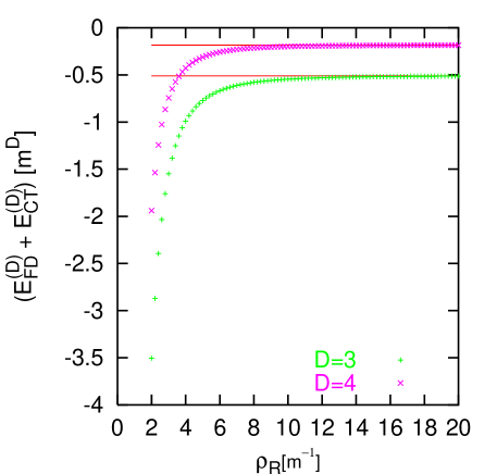
Figure 1: Renormalized $D=2+1$ and $D=3+1$ Feynman Diagram energies in appropriate units of $m$ as functions of the return flux radius for $w=1/m$ and $\mathcal{F}=4.8$. The solid lines correspond to the energies without the return flux.

In Fig. 2, we show the integrand of the phase shift part of the energy, eqs. (18, 19), in both the embedded configuration and the flux tube configuration, for two fixed values of $R$. The details of the calculation of the phase shifts of the non–zero flux configuration may be found in Appendix A.1. We observe that the integrands disagree only for small values of the momentum, at which the fermion is sensitive to the presence of the spread-out return flux. The integrand for the embedded configuration oscillates around the integrand of the flux tube configuration with an amplitude that decreases as $k$ increases. The region of disagreement gets pushed to smaller values of $k$ as $R$ increases. In the limit $R\to\infty$, we find that the phase shift contribution to the energy is identical for the embedded and the flux tube problems. Analogous results hold in $D=3+1$ because the integrand differs from that in $D=2+1$ only by a background-independent function of $k$, cf. eqs. (18) and (19).

         

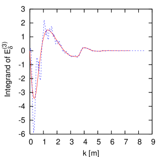
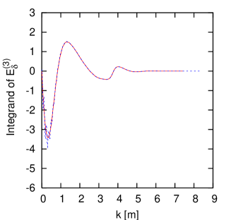
Figure 2: Integrand of the phase shift contribution to the energy in $D=2+1$ for $R=6/m$ (left panel) and $R=26/m$ (right panel). The solid lines correspond to the isolated flux tube problem and the dashed lines to the embedded problem.

Since the energy in the embedded problem approaches the energy in the isolated flux tube problem, for computational efficiency we can use the phase shifts in the background of the isolated flux tube to compute the energy, with the implicit understanding that there is a spread-out return flux present that does not affect the energy.

6 Results

In this Section we discuss our numerical results in more detail. The central issue will be the energy of the flux tube. We will also consider its energy and charge densities, as obtained from the embedded problem, and compare our results to the derivative expansion.

6.1 Energy

As already argued in the previous Section, we can compute the energy of a magnetic flux tube in three and four dimensions either independently or by embedding it in a zero–net–flux configuration. We then use scattering data to compute the vacuum polarization energy. Of course, there are other (approximate) methods to compute the vacuum polarization energy of such a configuration, most notably the derivative expansion [4, 24, 25], which represents an expansion in derivatives of the magnetic field. However, this expansion has recently been criticized, in particular in the four-dimensional case [9]. Since our approach is exact, we can easily test the validity of the derivative expansion. In addition, we may compare our results to a perturbative expansion in the magnitude of the magnetic field. For the Gaußian flux tube, eq. (6) we can formulate both expansions by varying the width, $w$ under appropriate constraints.

6.1.1 Derivative Expansion

As its width approaches infinity, a Gaußian flux tube with a fixed value of magnetic field at its center approaches a spatially constant magnetic field, for which the derivative expansion is reliable. Therefore, to compare with the derivative expansion, we compute the total energy of configurations with varying $w$ and fixed $B_{\rm G}(0)$ for the Gaußian magnetic field, eq. (5). The flux, eq. (6), is not held fixed in this approach.

In $D=2+1$, the derivative expansion of the unrenormalized one-loop vacuum polarization energy is given by [4, 24]

$$E^{(3)}_{{\rm vac},DE}-E^{(3)}_{\rm CT}=E^{(3)}_{{\rm DE},0}+E^{(3)}_{{\rm DE},2}+\ldots\,,$$ (36)

to next-to-leading order in the derivative, where

$$E^{(3)}_{{\rm DE},0} = \int d^{2}x\frac{|eB|^{3/2}}{4\pi^{3/2}}\int_{0}^{\infty}dse^{-sm^{2}/|eB|}s^{-3/2}\left(\coth(s)-\frac{1}{s}\right)\,,$$

$$E^{(3)}_{{\rm DE},2} = \frac{1}{4}\int d^{2}x|\nabla(eB)|^{2}|4\pi eB|^{-3/2}\int_{0}^{\infty}dse^{-sm^{2}/|eB|}s^{-1/2}\frac{d^{3}(s\coth s)}{ds^{3}}\,.$$ (37)

Note that the above expressions are for four-component fermions in the loop, which give twice the result for two-component spinors. Scaling the spatial integration variable by $\xi=x/w$ straightforwardly yields $E^{(3)}_{{\rm DE},0}\propto w^{2}$ and $E^{(3)}_{{\rm DE},2}\propto w^{0}$. The counterterm contribution to the energy is also proportional to $w^{2}$. We stress that keeping $B(0)$ fixed is important to obtain this simple power law behavior. (Taking the limit differently, for example with the flux fixed, the proper-time integrals in eqs. (37) would induce more complicated dependences on $w$.) For the special case of the Gaußian flux tube we find

$$E^{(3)}_{\rm CT}=-\frac{e^{2}B_{\rm G}^{2}(0)w^{2}}{24m}\,.$$ (38)

We add the counterterm to get the renormalized derivative expansion

$$E^{(3)}_{{\rm vac},DE}=E^{(3)}_{\rm CT}+E^{(3)}_{{\rm DE},0}+E^{(3)}_{{\rm DE},2}+\ldots\,.$$ (39)

It is straightforward to verify that this expression satisfies the on-shell renormalization condition that we imposed on our scattering data result in subsection 3.1. The first two terms on the right hand side of eq. (39) are proportional to $w^{2}$, while the last term is independent of $w$. All omitted terms contain more derivatives, and thus they vanish as $w\to\infty$.

In $D=3+1$, the next-to-leading order derivative expansion of the renormalized one-loop energy is

$$E^{(4)}_{{\rm vac},DE}=E^{(4)}_{{\rm DE},0}+E^{(4)}_{{\rm DE},2}\,+\ldots,$$ (40)

where [25]

$$E^{(4)}_{{\rm DE},0} = \int d^{2}x\frac{|eB|^{2}}{8\pi^{2}}\int_{0}^{\infty}dse^{-sm^{2}/|eB|}s^{-2}\left(\coth(s)-\frac{1}{s}-\frac{s}{3}\right)\,,$$

$$E^{(4)}_{{\rm DE},2} = -\int d^{2}x|\nabla(eB)|^{2}|32\pi^{2}eB|^{-1}$$

$$\hskip 56.9055pt\times\int_{0}^{\infty}dse^{-sm^{2}/|eB|}\left(1-4\coth^{2}s+3\coth^{4}s+\frac{3\coth s}{s}(1-\coth^{2}s)\right)\,.$$

Again we have $E^{(4)}_{{\rm DE},0}\propto w^{2}$ and $E^{(4)}_{{\rm DE},2}\propto w^{0}$, with higher orders going as inverse powers of $w$.

In Fig. 3, we compare our exact result $E^{(D)}_{\rm vac}$ with the derivative expansion approximation $E^{(D)}_{{\rm vac},DE}$ for different values of $eB_{\rm G}(0)$, and find excellent agreement for widths larger than 1. There appears to be no qualitative difference $D=2+1$ and $D=3+1$. However, had we not included the counterterm in $D=2+1$, as is done in [9], we would be effectively imposing a different renormalization condition from the one in $D=3+1$, and would see a qualitative difference between these two cases. As we will see below, the extra contribution from the off-shell scheme can dominate the underlying result. In particular, if this scheme is consistently imposed both exactly and in the derivative expansion, this dominant contribution can obscure differences between the exact result and the derivative expansion in cases where the derivative expansion is not valid.

         

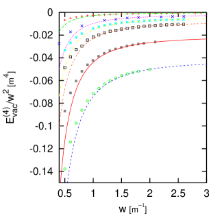
Figure 3: Renormalized one-loop energies in $D=2+1$ (left panel) and $D=3+1$ (right panel), for fixed values of the magnetic field at the origin, as a function of the width of the Gaußian flux tube. The lines correspond to the derivative expansion to lowest nontrivial order in the derivative. From top to bottom, $eB_{\rm G}(0)/m^{2}=1.1,2,2.5,3,4,5$.

6.1.2 Fixed Flux

We next turn to such a limit, which is the case of configurations for which the flux, rather than the magnetic field at the origin, is held fixed as the width approaches infinity. This limit was considered in ref. [9]. In this case the energy of the flux tube goes to zero as $w$ goes to infinity, and it is the perturbation expansion, rather than the derivative expansion, that becomes exact.

First consider the classical energy, eq. (8),

$$E_{\rm cl}=\frac{\pi\mathcal{F}^{2}}{e^{2}}\int_{0}^{\infty}\frac{dr}{r}\,\left(\frac{df_{G}(r)}{dr}\right)^{2}=\frac{\pi\mathcal{F}^{2}}{e^{2}w^{2}}\,,$$ (42)

for the Gaußian flux tube, eq. (5). For large widths, it goes to zero like $1/w^{2}$. In this limit, the magnetic field becomes weak, as can easily be seen from eq. (6). Hence the dominant contribution to the vacuum polarization energy comes from the two-point function. In $D=2+1$, the unrenormalized two-point energy can be expressed as a series in $1/w^{2}$. The leading term proportional to $1/w^{2}$ turns out to be exactly equal to minus the counterterm energy in the on–shell subtraction scheme. Thus only the subleading term survives in the renormalized two-point energy. For a Gaußian flux tube,

$$E^{(3)}_{\rm FD} = \frac{\mathcal{F}^{2}}{6mw^{2}}\left(1-\frac{1}{5m^{2}w^{2}}+\mathcal{O}(1/w^{4})\right)$$

$$E^{(3)}_{\rm FD}+E^{(3)}_{\rm CT} = -\frac{\mathcal{F}^{2}}{30m^{3}w^{4}}+\mathcal{O}(1/w^{6})\,.$$ (43)

For large widths, renormalization not only changes the sign of the one-loop energy, but also the rate at which zero is approached. The renormalized results in $D=3+1$ are similar to the results in $D=2+1$:

$$E^{(4)}_{\rm FD}+E^{(4)}_{\rm CT}=-\frac{\mathcal{F}^{2}}{30\pi m^{2}w^{4}}+\mathcal{O}(1/w^{6})$$ (44)

for the Gaußian flux tube. In the limit $w\rightarrow\infty$, the total energy for both $D=2+1$ and $D=3+1$ vanishes. This result enables us to introduce a return flux in the embedded problem without changing the energy.

While such fixed flux configurations are well approximated by the perturbative expansion, they are inappropriate to test the derivative expansion, as was done in ref. [9]. Since the magnitude of the magnetic field at the center of the vortex then depends on the width, so too will the proper-time integrals in eqs. (37, 6.1.1), and there is no longer any reason to expect that the the two-derivative contribution is less important than the no-derivative contribution for large widths.

In Fig. 4, we plot the exact one-loop energies for various values of the flux as a function of the width. We normalize the energies in units of $\mathcal{F}^{2}$ so that all differences between the different fluxes are due to three-point and higher contributions. We compare the energies with the leading order two-point energies and find good agreement for large widths. As the flux increases, we need to go to larger widths to get a weak magnetic field everywhere, cf. eq. (6). Hence the agreement with the leading order two–point function contribution to the energy sets in at larger widths when the flux increases.

         

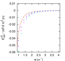
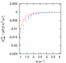
Figure 4: Renormalized fermion vacuum polarization energy in units of $\mathcal{F}^{2}$ as a function of the width, for various fixed values of the flux $\mathcal{F}$ (2.5, 4.5, 6.5, 8.5 from top to bottom) in the Gaußian flux tube. The full line represents the two-point function contribution. The left panel is for $D=2+1$ and the right panel for $D=3+1$.

6.1.3 Further Comments

Methods similar to our phase shift calculation have been used in ref. [26]. However, in this calculation infinite quantities are used without proper renormalization, such as eq. (26) of [26] for $D=3+1$. Although convergent results are reported, we believe that they are an artifact of taking a low, fixed upper limit in the sum over channels. Instead, this limit should scale with the momentum $k$. By keeping more terms in the sum, one should see this divergence.

n Ref. [8] a step function background $B(r)$ was studied in $D=2+1$ dimensions. In order to separate divergent contributions to the vacuum polarization energy the authors of Ref. [8] extracted the asymptotic behavior of the Jost function and identified that with pieces in the heat kernel expansion. Instead of using on-shell renormalization conditions, the renormalization is defined by requiring that the renormalized vacuum polarization energy vanishes in the limit where the fermion becomes infinitely heavy. However, this requirement is not sufficient to uniquely determine the renormalization scheme, as has been noted in [27]. As a result, we cannot make a quantitative comparison with our calculation, but qualitatively, our results seem to agree in the sense that they also find a negative vacuum polarization energy. Since different renormalization conditions amout to different contributions from the positive definite counterterm, eq. (11), this agreement may be not be conclusive.

6.2 Energy Density

So far we have only discussed the total vacuum polarization energy of the flux tube. We have argued that it is preferable to consider a flux tube embedded in system with no net flux, where the region carrying the return flux is well separated from the flux tube core. In this Section we make this argument more precise by studying the radial density of the vacuum polarization energy. We will observe that the contribution to the energy density from the central flux tube and the return flux can clearly be distinguished, giving a unique definition for the energy of the central flux tube alone. Numerical evaluation shows that it equals the energy of the non-embedded flux tube that we computed in Section 5. We will also take the opportunity to compare our results for the energy density with the derivative expansion approximation, which has recently been discussed in ref. [9].

We define the radial energy density in terms of the renormalized vacuum expectation value of the energy-momentum tensor $\hat{T}_{\mu\nu}(x)$ by $\epsilon(r)=2\pi r\langle\hat{T}_{00}(x)\rangle$. In Appendix B we discuss $\hat{T}_{00}(x)$ in more detail, with particular attention to total derivative terms. The radial energy density $\epsilon(r)$ has been normalized so that the total energy is $E^{(D)}_{\rm vac}=\int_{0}^{\infty}dr\,\epsilon(r)$. In figure 5 we show the energy density for the configuration defined in eq. (34). As the separation $R$ between $B_{G}$ and $B_{R}$ increases, the contribution from the return flux region decreases, going to zero as $R\to\infty$. In addition, we observe that the energy density localized around the flux tube at $r=0$ remains unchanged when we increase the separation. That part of the energy density does not depend on whether the return flux configuration is included once $B_{G}$ and $B_{R}$ are well separated. Finally, the intermediate region in which the density $\epsilon(r)$ vanishes becomes more pronounced.

         

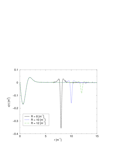
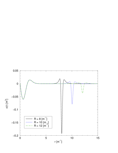
Figure 5: The vacuum polarization energy densities of configurations with zero net flux as functions of the separation $R=8,10,12/m$ between $B_{G}$ and $B_{R}$. We choose $eB(0)=4m^{2}$ and $w=1.5/m$. The left and right panels show $D=2+1$ and $D=3+1$, respectively.

Once the region with $\epsilon(r)\approx 0$ is large enough we can clearly distinguish between the energy densities due to $B_{G}$ and $B_{R}$.

In figure 6 we show the renormalized Feynman diagram and scattering data contributions to the energy density.

         

         

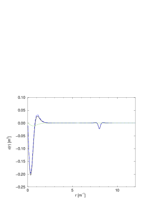
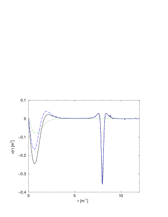
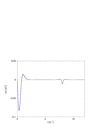
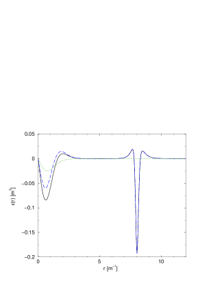
Figure 6: Feynman diagram (dashed) and scattering data (dotted) contributions to the energy density for configurations with zero net flux. Their sum (full) is the full vacuum polarization energy density. Two cases are considered, $w=0.75/m$ (left panel) and $w=1.5/m$ (right panel), both with $eB(0)=4m^{2}$ and $R=8/m$, for $D=2+1$ (top) and $D=3+1$ (bottom).

We observe that for small widths of the central Gaußian flux tube, the scattering data contributions are negligible, while for larger widths they contribute as much as 30% to the total energy. Note that $B(0)$ is kept fixed. We also see that the scattering data contribution to the energy density essentially vanishes in the return flux region. This numerical result reflects a cancellation when summing over many orbital angular momentum channels; the individual channels themselves contain sizable contributions to the energy density in the vicinity of $r=R$. This result is to be expected: Since the return flux region extends to large radii, large angular momentum channels contribute to the energy density there. We find that several hundred channels must be summed for convergence.

The computation of the Feynman diagram contribution to the energy density does not rely on any conditions for the background field. Since the energy densities are well approximated by their Feynman diagram contributions for small widths, we can compare energy densities for configurations with and without $B_{R}$ in cases with small $w$. This comparison is shown in figure 7.

         

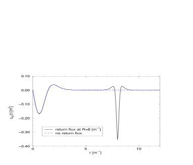
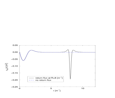
Figure 7: Renormalized Feynman diagram contributions to the energy density for configurations with and without return flux for $w=1.5/m$, $eB(0)=4m^{2}$ and $R=8/m$, in the case of zero net flux. The left and right panels show $D=2+1$ and $D=3+1$ respectively.

Integrating the energy density over the region of return flux, we find that even at moderate separation it only contributes a small amount to the vacuum polarization energy. However, as figure 7 illustrates, this result arises from the cancellation of significant positive and negative densities in this region. It is not surprising that the energy density of the return flux is nontrivial: We keep $B(0)$ fixed, so as the width of the flux tube increases, its flux does too, according to eq. (6). To have zero net flux, the amplitude of the return flux piece must increase when $w$ gets larger and $R$ remains unchanged, as can be seen from eq. (32).

To compare the results for the exact vacuum polarization energy density with the derivative expansion, we must identify the energy density in that approximation. The derivative expansion for the vacuum polarization energy, eqs. (37,6.1.1), originates from the expansion for the action. Hence simply omitting the radial integrals in those expressions can only be expected to yield an approximation to the action density. Formally we may write

$$E_{{\rm DE},n}^{(D)}=\int_{0}^{\infty}drr\left(\frac{dB(r)}{dr}\right)^{n}f^{(D)}_{n}(B(r))\,,$$ (45)

with $f_{n}^{(D)}(B(r))$ to be read off eqs. (37,6.1.1) for $n=0,2$. As discussed in Appendix B the action and energy densities differ by total derivatives, which vanish when integrated over space. These total derivates only affect the orders $n\geq 2$ because for constant magnetic fields both the energy and action density should be constant. Thus only $E_{\rm DE,2}^{(D)}$ is affected at next-to-leading order. The direct determination of this total derivate term involves all orders in perturbation theory and seems difficult to accomplish. We therefore introduce the parameter $\xi$ to define the energy density at next-to-leading order in the derivative expansion,

$$\epsilon_{\rm DE}^{(D)}(r)=r\left[f^{(D)}_{0}(B(r))+\left(\frac{dB(r)}{dr}\right)^{2}f^{(D)}_{2}(B(r))\right]+\xi\frac{d}{dr}\left[r\frac{dB(r)}{dr}f^{(D)}_{2}(B(r))\right]\,,$$ (46)

where the case $\xi=0$ corresponds to the the derivative expansion for the action density. Then we can fit for $\xi$ by comparing to the exact result $\epsilon(r)$.

For the derivative expansion to be applicable we need to consider increasing widths $w$ with $B(0)$ unchanged. As discussed above, for such configurations we may not omit the scattering data contribution and therefore we consider configurations with zero net flux. The comparison of the energy density is displayed in figure 8.

         

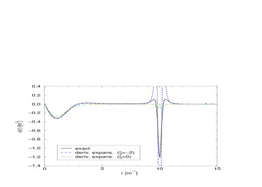
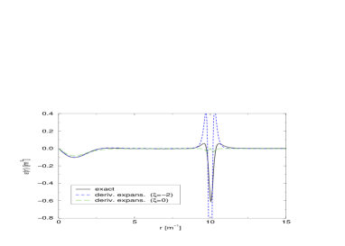
Figure 8: Comparison between the computed energy density for configurations with zero net flux and the derivative expansion approximation. We take $w=2.5/m$, $eB(0)=4m^{2}$ and $R=10/m$ and consider the case without ($\xi=0$) and with ($\xi=-2$) total derivative term, (46). The left and right panels show $D=2+1$ and $D=3+1$, respectively.

We find reasonable agreement with the derivative expansion for sizable $w$ in the region of the central flux tube for both $D=2+1$ and $D=3+1$, where the magnetic field is slowly varying. Since we keep the position and the width of the return flux unchanged as we increase the width of the flux tube, we do not expect the derivative expansion to match the exact result in the vicinity of the return flux. From figure 8 we observe that $\xi=-2$ appears optimal for both $D=2+1$ and $D=3+1$.

         

         

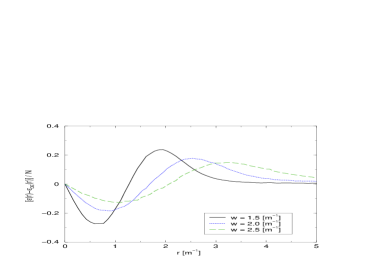
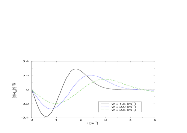
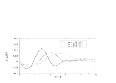
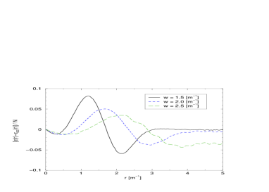
Figure 9: The difference between the exact result and derivative expansion for the energy density in the vicinity of the central flux tube as a function of its width. These differences are always normalized to maximal absolute value of the exact energy density in the flux tube region. The left and right panels show $D=2+1$ and $D=3+1$, respectively. Also we consider $\xi=0$ (top) and $\xi=-2$ (bottom). Note the different scale of the latter.

This result confirms the assertion of Appendix B that the energy and action densities differ by total derivatives.

In fig. 9 we display the normalized difference $\left[\epsilon(r)-\epsilon_{\rm DE}(r)\right]/N$ with the normalization factor $N={\rm max}\{|\epsilon(r)|,r\leq 2w\}$ for various widths $w$. Of course, we have to ensure that there is no overlap with the return flux when we consider large values of $w$. For $w=2.5/m$ (the largest value we consider) this requirement is well satisfied for $R=10/m$. As expected, this normalized difference decreases as $w$ increases. A non-zero difference extends to larger $r$ as $w$ increases, reflecting the growing extension of the central flux tube. Again, we observe that the inclusion of the total derivative term improves the agreement with derivative expansion approximation. As can be clearly seen from fig. 9, even though the difference between the derivative expansion and the exact result for the density is quite sizable at small widths, it is close to a total derivative, which explains the good convergence of the derivative expansion for the total energy, even at moderate widths $w$.

To summarize, we find reasonable agreement for the energy density between our exact results and the derivative expansion approximation at next–to–leading order for both $D=2+1$ and $D=3+1$. Our result for the $D=3+1$ case contradicts the findings of ref. [9]. That work uses the world-line formalism as a non-perturbative computation of the action density and finds a discrepency with the derivative expansion approximation in $D=3+1$. We note that this discrepency cannot originate from the total derivative terms in the derivative expansion, since that work also considered the action density. Also, we have seen that the total derivative terms affect $D=2+1$ and $D=3+1$ similarly.

On the other hand, in ref. [9], a fixed flux sequence of magnetic fields has been employed to test the derivative expansion. We have already argued that a fixed peak magnetic field configuration should be used instead. Thus one might wonder why ref. [9] finds a good agreement for a fixed flux configuration in the $D=2+1$ case. We ascribe this result to the choice of renormalization scheme, in which the finite counterterm has been omitted. For both the energy density and the total energy, we find that the inclusion of the counterterm leads to considerable changes in the case of $D=2+1$. Since the counterterm only affects the second-order contribution to the energy and energy density, it is sufficient to consider the corresponding Feynman diagrams to study the influence of renormalization for $D=2+1$. This comparison is shown in figure 10.

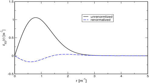
Figure 10: Comparison of renormalized and unrenormalized $2^{\rm nd}$ order Feynman diagram contribution to the energy density for $D=2+1$. For simplicity we set $B_{R}\equiv 0$ and take $eB(0)=4m^{2}$ and $w=1.5/m$.

The renormalized energy density is about an order of magnitude smaller and of opposite sign than the unrenormalized one. Thus if one does not add a counterterm in $D=2+1$, the leading order term $E_{\rm DE,0}$ contains a large, though unphysical, contribution to the energy and energy density. But then the comparision with the derivative expansion merely tests the agreement in this term, which masks the underlying differences between the exact and approximate results. We thus conjecture that the authors of ref. [9] would also have found disagreement between their results and the derivative expansion approximation in $D=2+1$ if they had imposed the on–shell renormalization condition for their fixed flux background configuration. In substance, the (dis)agreements between the derivative expansion and the world line formalism observed in ref. [9] do not reflect short-comings of either of these approaches but merely the inappropriateness of the fixed flux configuration to check these approaches against each other.

6.3 Charge Density

In this subsection, we concentrate on ${\rm QED}_{2+1}$ with a single two–component fermion since for a four–component fermion the charge density vanishes identically. Since the charge density is a component of a conserved current, it is not renormalized by quantum effects. Therefore, we can diagonalize the Dirac Hamiltonian within a Hilbert space that contains a large but finite number of states. We then simply compute

$$\rho(r)=r\,\sum_{j}{\rm sign}(\epsilon_{j})\,\int_{0}^{2\pi}d\varphi\,\Psi_{j}^{\dagger}(\vec{x\,})\Psi_{j}(\vec{x\,})$$ (47)

where $\epsilon_{j}$ and $\Psi_{j}(\vec{x\,})$ are the eigenvalues and eigenspinors respectively. The technical details of this calculation are summarized in Appendix C. We have verified the stability of the sum (47) with respect to variation of the cut-off that restricts the Hilbert space. In figure 11 we display the resulting densities for the background field defined in eq. (33).

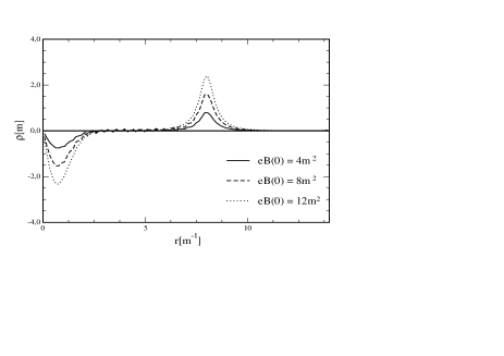
Figure 11: The charge density computed from eq. (47) for various locations of the return flux and strength of the magnetic field. The return flux is at $6/m$ in the left panel and at $8/m$ in the right panel.

Clearly the charge density is localized at the regions of the flux tube and return flux. As these regions are separated, so are the peaks of the charge density. While the total charge vanishes, the integral up to some intermediate point $r_{M}\approx R/2$, with $\rho(r_{M})\approx 0$ gives

$$\int_{0}^{r_{M}}dr\,\rho(r)\approx-\frac{\mathcal{F}}{2}\,$$ (48)

exactly as expected from a single vortex located at $r=0$ [6, 5]. In figure 12, we display the charge density obtained from the same calculation for background fields without return flux.

       

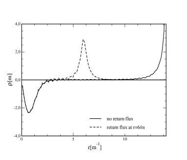
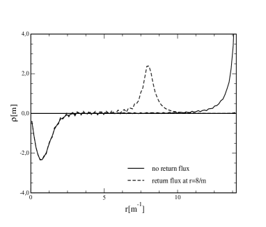
Figure 12: The charge density computed from eq. (47) with and without return flux. In both cases $eB(0)=12m^{2}$.

We observe that in the vicinity of the central vortex, the resulting densities with and without return flux are identical, again verifying that we may consider the vortex as part of a configuration with vanishing total flux.

It is illuminating to study the charge density using the Green’s function formalism as we did for the energy density in the previous Section, using the results of Appendix A. For background configurations with vanishing total flux, the solutions to Dirac equation come in pairs with opposite signs of the energy eigenvalues. From equations (LABEL:poseng) and (69) in Appendix A we then find that the scattering states obey

$$\sum_{j}{\rm sign}(\epsilon_{j})\,\frac{1}{2}\left[\Theta(|\epsilon_{j}|-\delta)-\Theta(|\epsilon_{j}|+\delta)\right]\int_{0}^{2\pi}d\varphi\,\Psi_{j}^{\dagger}(\vec{x\,})\Psi_{j}(\vec{x\,})=0\,.$$ (49)

for arbitrarily small but non–vanishing $\delta$. Hence they do not contribute to the charge density. Of course, this argument applies to any order of the Born expansion as well. However, to apply our Green’s function formalism we have to subtract enough Born terms that integrations in the complex momentum plane become well defined. For the charge density in $D=2+1$ only the first-order subtraction is required. The corresponding Feynman diagram gives

$$\rho_{\rm FD}(r)=r{\cal F}\int_{0}^{\infty}dp\left[\int_{0}^{\infty}dr^{\prime}\,\frac{df(r^{\prime})}{dr^{\prime}}\,J_{0}(pr^{\prime})\right]{\rm arctan}\left(\frac{p}{2m}\right)J_{0}(pr)\,.$$ (50)

Since we argued that the scattering Green’s function does not contribute to the charge density we expect the charge to be given exactly by this Feynman diagram. This result is confirmed by numerical calculations, shown in figure 13. We also compare to the local contribution, $\frac{{\cal F}}{2}\frac{df(r)}{dr}$, which is the leading term of the derivative expansion to $\rho_{\rm FD}(r)$.

     

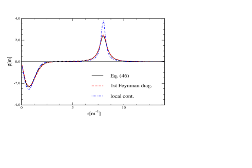
Figure 13: The charge density computed from the Feynman diagram (50) compared to the calculation from eq. (47) and the local contribution $\frac{{\cal F}}{2}\frac{df(r)}{dr}$. Here $eB(0)=12m^{2}$ and the return flux is at $8/m$.

We see that the charge density contains sizable non–localities, mostly in the vicinity of the return flux where the background is not slowly varying.

7 Summary

We have studied exact one-loop quantum energies and energy densities of static electromagnetic flux tubes in three and four spacetime dimensions. To this order only fermion fluctuations contribute to the vacuum polarization energy and energy density, which we compute exactly from scattering data. In general, this quantum contribution contains ultraviolet divergences and an important feature of our approach is that it allows us to impose the standard renormalization conditions of perturbative quantum electrodynamics. Even though the calculation in three spacetime dimensions does not suffer from such divergences, a meaningful comparison between three and four dimensions can only be made when identical renormalization conditions are imposed. Thus we must include a finite renormalization of the three-dimensional result. Furthermore, the use of scattering data to compute the vacuum polarization energy of an individual flux tube leads to subtleties arising from the long-range potential induced by the flux tube background, which does not satisfy the standard conditions of scattering theory. Consequently, the scattering data do not necessarily have the standard analytic properties and the phase shifts are discontinuous at small momenta. We have circumvented these problems by considering field configurations in which the flux tube is embedded with a well-separated return flux so that the total flux vanishes. We have constructed a limiting procedure in which this return flux does not contribute to the energy, enabling us to compute the energy of an isolated flux tube. While the return flux can give a nontrivial contribution to the charge and energy densities (which integrates to zero in the case of the energy density), such contributions are well separated from the flux tube and thus easily identified. Thus we have an unambiguous definition of the energy and charge of the isolated flux tube even in the embedded configuration. This embedding is analogous to considering a kink-antikink rather than an isolated kink to avoid boundary effects in one dimensional $\phi^{4}$ theory [16].

We do not see qualitative differences between three and four dimensions for either the energy or energy density, once identical renormalization conditions have been imposed. However, we stress that renormalization in the case of three dimensions proved essential to this result because the (finite) counterterm contribution turned out to be large, thus causing sizable cancellations in the final result.

We have tested various approximation schemes to the vacuum polarization energy of the flux. Though we have observed convergence of the perturbative expansion for small fluxes, we have concentrated on the derivative expansion. While we find good agreement between our exact calculation and the derivative expansion approximation for the total energy, there are discrepancies for the energy density, which arise because the derivative expansion result is an approximation to the effective action, which differs from the appropriate matrix element of the energy momentum tensor by a total derivative.

This study gives an initial step toward understanding flux tubes and vortices in more complicated theories. The next step would be to consider the complete $U(1)$ model, including a Higgs field with spontaneous symmetry breaking, which would describe flux tubes in a Type II superconductor. It could then be generalized to non-Abelian gauge bosons for the study of $Z$-strings in the Standard Model, which are flux tubes in the $Z$ gauge boson field. The methods developed here could then be used to determine whether quantum corrections stabilize the classically unstable $Z$-string.

Acknowledgments

We gratefully acknowledge helpful discussions with G. V. Dunne, E. Farhi, H. Gies and R. L. Jaffe. N. G. was supported in part by the Vermont Experimental Program to Stimulate Competitive Research (VT-EPSCoR). V. K. is supported in part by the U.S. Department of Energy (D.O.E.) under cooperative research agreements DF-FC02-94ER40818 and DE-FG02-92ER40716. O.S. was supported by the Deutsche Forschungsgemeinschaft under grant DFG Schr 749/1-1. This work is also supported in part by funds provided by the U.S. Department of Energy (D.O.E.) under cooperative research agreement DF-FC02-94ER40818.

Appendix A Energy Density from Green’s Function

In this Appendix we describe the construction of the exact fermion Green’s function in the flux tube background in terms of scattering data. We then use it to compute the quantum energy density due to the fermion fluctuations.

We will begin by considering four–component Dirac spinors $\Psi$ in $D=3+1$ dimensions. The calculation for two–component Dirac spinors in $D=2+1$ dimensions is then a simple manipulation. For the electromagnetic field $A^{\mu}=(0,A_{\varphi}\,\hat{e}_{\varphi})^{\mu}$, the $4\times 4$ Dirac equation decomposes into $2\times 2$ blocks

$$H\Psi=\begin{pmatrix}m&H_{2}\cr H_{2}&-m\end{pmatrix}\Psi=\omega\Psi\,,$$ (51)

where we now use the Bjorken–Drell representation for the Dirac matrices. Since the system is translationally invariant in the $z$ direction, we can choose $\Psi$ to be an eigenstate of $z$ momentum with eigenvalue $p$. Then the $2\times 2$ block becomes

$$H_{2} = \begin{pmatrix}\ p\ &\ L^{\dagger}\ \cr L&-p\end{pmatrix},$$ (52)

$$L = -i{\rm e}^{i\varphi}\left[\partial_{r}+eA_{\varphi}(r)+\frac{i}{r}\partial_{\varphi}\right],\quad L^{\dagger}=-i{\rm e}^{-i\varphi}\left[\partial_{r}-eA_{\varphi}(r)-\frac{i}{r}\partial_{\varphi}\right]\,.$$ (54)

where $r=\sqrt{x^{2}+y^{2}}$. Accordingly we decompose the four-spinor into two two-spinors $\Psi=\begin{pmatrix}\xi~{}~{}\eta\end{pmatrix}$, which obey the second-order equations

$$H_{2}^{2}\eta=\left(\omega-m\right)H_{2}\xi=\left(\omega^{2}-m^{2}\right)\eta\hbox{\quad with \quad}H_{2}^{2}=\begin{pmatrix}p^{2}+L^{\dagger}L&0\cr 0&LL^{\dagger}+p^{2}\end{pmatrix}$$ (55)

and similarly for $\xi$. Thus we only have to diagonalize $L^{\dagger}L$ and $LL^{\dagger}$ by solving

$$L^{\dagger}L\left[g_{\ell}^{(1)}(r){\rm e}^{i\ell\varphi}\right] = {\rm e}^{i\ell\varphi}\left\{-\partial_{r}^{2}-\frac{1}{r}\partial_{r}+\frac{\left(l-h(r)\right)^{2}}{r^{2}}-\frac{h^{\prime}(r)}{r}\right\}g_{\ell}^{(1)}(r)$$ (56)

$$= k^{2}\left[g_{\ell}^{(1)}(r){\rm e}^{i\ell\varphi}\right]$$ (57)

$$LL^{\dagger}\left[g_{\ell}^{(2)}(r){\rm e}^{i(\ell+1)\varphi}\right] = {\rm e}^{i(\ell+1)\varphi}\left\{-\partial_{r}^{2}-\frac{1}{r}\partial_{r}+\frac{\left(l+1-h(r)\right)^{2}}{r^{2}}+\frac{h^{\prime}(r)}{r}\right\}g_{\ell}^{(2)}(r)$$

$$= k^{2}\left[g_{\ell}^{(2)}(r){\rm e}^{i(\ell+1)\varphi}\right]\,,$$

where $h(r)=erA_{\varphi}(r)=\mathcal{F}f(r)$, as in eqs. (2) and (4). Note that $\ell$ takes positive and negative integer values.

The equations in (56) represent problems in ordinary scattering theory, with potentials

$$V_{1}^{(\ell)}(r) = \frac{h(r)^{2}}{r^{2}}-2\ell\frac{h(r)}{r^{2}}+\frac{h^{\prime}(r)}{r}$$ (59)

$$V_{2}^{(\ell)}(r) = \frac{h(r)^{2}}{r^{2}}-2(\ell+1)\frac{h(r)}{r^{2}}-\frac{h^{\prime}(r)}{r}$$ (60)

and their solutions possess the standard analytic properties in the complex $k$ plane if these potentials obey the usual conditions[15]. This is the case for the embedded flux tube, where we can use the techniques of ref. [23] to construct solutions for $g_{\ell}^{(i)}$ that obey the Jost and scattering boundary conditions. Since the rotation to the imaginary $k$ axis removes the explicit contribution of any bound states to the energy density[8], it is sufficient to concentrate on the scattering solutions.

We construct the scattering eigenspinors of eq. (51) in analogy to the plane wave solution to a free Dirac field. The eigenvalues of the full Dirac problem are $\omega=\pm\sqrt{k^{2}+p^{2}+m^{2}}$, and we define the positive quantity $E=\sqrt{k^{2}+p^{2}+m^{2}}$. Spinors with eigenvalue $\omega=+E$ are

$$\Psi_{\ell}^{(1)}(k,p;r,z) = \sqrt{\frac{E+m}{4\pi E}}{\rm e}^{ipz}\begin{pmatrix}g_{\ell}^{(1)}(k;r){\rm e}^{i\ell\varphi}\cr 0\cr\frac{p}{E+m}g_{\ell}^{(1)}(k;r){\rm e}^{i\ell\varphi}\cr\frac{L}{E+m}g_{\ell}^{(1)}(k;r){\rm e}^{i\ell\varphi}\end{pmatrix}$$ (61)

$$= \sqrt{\frac{E+m}{4\pi E}}\,{\rm e}^{i\ell\varphi}{\rm e}^{ipz}\begin{pmatrix}g_{\ell}^{(1)}(k;r)\cr 0\cr\frac{p}{E+m}g_{\ell}^{(1)}(k;r)\cr\frac{-i{\rm e}^{i\varphi}}{E+m}L_{r}^{(-)}g_{\ell}^{(1)}(k;r)\cr\end{pmatrix}$$ (63)

$$\Psi_{\ell}^{(2)}(k,p;r,z) = \sqrt{\frac{E+m}{4\pi E}}\,{\rm e}^{i(\ell+1)\varphi}{\rm e}^{ipz}\begin{pmatrix}0\cr-g_{\ell}^{(2)}(k;r)\cr\frac{i{\rm e}^{-i\varphi}}{E+m}L_{r}^{(+)}g_{\ell}^{(2)}(k;r)\cr\frac{p}{E+m}g_{\ell}^{(2)}(k;r)\end{pmatrix}\,,$$

where we have introduced the linear differential operators

$$L_{r}^{(+)}=\partial_{r}+\frac{\ell+1-h(r)}{r}\qquad{\rm and}\qquad L_{r}^{(-)}=\partial_{r}-\frac{\ell-h(r)}{r}\,.$$ (65)

These equations exhibit the symmetry

$$g_{-\ell-1}^{(1)}(k;r)[h]=g_{\ell}^{(2)}(k;r)[-h]\,.$$ (66)

Similarly, the spinors for the anti–fermions with eigenvalues $\omega=-E$ are

$$\Psi_{\ell}^{(3)}(k,p;r,z) = \sqrt{\frac{E+m}{4\pi E}}{\rm e}^{i\ell\varphi}{\rm e}^{ipz}\begin{pmatrix}\frac{-p}{E+m}g_{\ell}^{(1)}(k;r)\cr\frac{i{\rm e}^{i\varphi}}{E+m}L_{r}^{(-)}g_{\ell}^{(1)}(k;r)\cr g_{\ell}^{(1)}(k;r)\cr 0\end{pmatrix}$$ (67)

$$\Psi_{\ell}^{(4)}(k,p;r,z) = \sqrt{\frac{E+m}{4\pi E}}\,{\rm e}^{i(\ell+1)\varphi}{\rm e}^{ipz}\begin{pmatrix}\frac{i{\rm e}^{-i\varphi}}{E+m}L_{r}^{(+)}g_{\ell}^{(2)}(k;r)\cr\frac{p}{E+m}g_{\ell}^{(2)}(k;r)\cr 0\cr g_{\ell}^{(2)}(k;r)\end{pmatrix}\,.\hskip 5.69046pt$$ (69)

Assuming the normalization condition for boson wavefunctions as in ref. [23]

$$\int_{0}^{\infty}rdr\,g_{\ell}^{(i)*}(k^{\prime};r)g_{\ell}^{(i)}(k,r)=\frac{\pi}{2}\delta(k^{\prime}-k)\qquad i=1,2$$ (70)

the spinors obey

$$\int d^{2}r\,\Psi_{\ell^{\prime}}^{(\alpha^{\prime})\dagger}(k^{\prime},p;r)\Psi_{\ell}^{(\alpha)}(k;r)=\delta_{\alpha^{\prime}\alpha}\delta_{\ell^{\prime}\ell}\frac{\pi}{2}\delta(k^{\prime}-k)\,.$$ (71)

The solutions in the two-dimensional case are obtained by setting $p=0$. Then the spinors are also eigenstates of ${\rm diag}(1,-1,-1,1)$, reflecting the decomposition of the four-spinor into two decoupled two-spinors.

We would like to compute the renormalized radial energy density,

$$\epsilon(r)=2\pi r\langle\Omega|\hat{T}_{00}(x)|\Omega\rangle_{\rm ren}\,.$$ (72)

Here $|\Omega\rangle$ denotes the vacuum of fluctuating fermions that are polarized by the background electromagnetic field, $A_{\mu}(x)$ and

$$\hat{T}_{00}(x)=\bar{\Psi}(x)\left(-i\gamma^{i}\partial_{i}+eA\hskip-6.00006pt/+m\right)\Psi(x)$$ (73)

is the energy field operator. The polarized vacuum is annihilated by the operators $a_{\ell}^{(s)}(k,p)$ and $b_{\ell}^{(s)}(k,p)$ that appear in the decomposition of the field operator

$$\Psi(x) = \int\frac{dp}{\sqrt{2\pi}}{\rm e}^{ipz}\,\int_{0}^{\infty}\frac{dk}{\sqrt{\pi E}}\sum_{\ell=-\infty}^{\infty}\sum_{s=1}^{2}\Big{[}\Psi_{\ell}^{(s)}(k,p;r)\,{\rm e}^{-iEt}\,a_{\ell}^{(s)}(k,p)$$ (75)

$$\hskip 199.16928pt+\Psi^{(s+2)}_{\ell}(k,p;r)\,{\rm e}^{iEt}\,b_{\ell}^{(s)\dagger}(k,p)\Big{]}\,.$$

Again, we have omitted potential bound state contributions.

The ultraviolet divergences in the matrix element (72) are canceled by counterterms that we determine by suitable renormalization conditions. These divergences are at most quadratic in the background field, $A_{\varphi}$. The Taylor expansion in $A_{\varphi}$ for $\left[\epsilon(r)\right]_{2}$, the radial energy density with the first two Born approximations subtracted, starts at cubic order and is free of ultraviolet divergences. We will therefore first compute $\left[\epsilon(r)\right]_{2}$ and in the next Appendix add back the subtracted pieces in form of Feynman diagrams combined with the counterterms. We obtain $\left[\epsilon(r)\right]_{2}$ using the standard anti-commutation relations for $a_{\ell}^{(s)}(k,p)$ and $b_{\ell}^{(s)}(k,p)$. Since the spinors $\Psi_{\ell}^{(s)}(k,p;r)$ obey the Dirac equation this yields

$$\left[\epsilon(r)\right]_{2}=-r\int_{0}^{2\pi}d\varphi\int\frac{dp}{2\pi}\int_{0}^{\infty}\frac{dk}{\pi}\sum_{\ell=-\infty}^{+\infty}\sum_{\alpha=1}^{4}\sqrt{k^{2}+p^{2}+m^{2}}\,\left[\Psi_{\ell}^{(\alpha)\dagger}(k,p;r)\Psi_{\ell}^{(\alpha)}(k,p;r)\right]_{2}\,.$$ (76)

We note that $L_{r}^{(-)}g_{\ell}^{(1)}(k;r)$ and $g_{\ell}^{(2)}(k;r)$ satisfy the same linear second order differential equation, as do $L_{r}^{(+)}g_{\ell}^{(2)}(k;r)$ and $g_{\ell}^{(1)}(k;r)$. To relate one solution to the other, we need to consider the boundary conditions. The radial functions that enter the Green’s functions (78) obey physical scattering boundary conditions [23]. Thus we identify

$$L_{r}^{(-)}g_{\ell}^{(1)}(k;r)=-ikg_{\ell}^{(2)}(k;r)\qquad{\rm and}\qquad L_{r}^{(+)}g_{\ell}^{(2)}(k;r)=ikg_{\ell}^{(1)}(k;r)\,,$$ (77)

which simplifies the sum in eq. (76) considerably. Our main objective is to express the right hand side of eq. (76) in terms of the Green’s functions for $g_{\ell}^{(1)}(k;r)$ and $g_{\ell}^{(2)}(k;r)$,

$$G^{(s)}_{\ell}(r,r^{\prime},k)=-\frac{2r}{\pi}\int_{0}^{\infty}dq\,\frac{g_{\ell}^{(s)*}(q;r)g_{\ell}^{(s)}(q;r^{\prime})}{(k+i\epsilon)^{2}-q^{2}}\,,\qquad s=1,2\,.$$ (78)

by noting that the imaginary part of the Green’s function at coincident points may be related to the wavefunctions,

$$\mathsf{Im}G_{\ell}^{(s)}(r,r,k)=\frac{r}{k}\,|g_{\ell}^{(s)}(k;r)|^{2}\,.$$

Collecting pieces finally yields the energy density

$$\left[\epsilon(r)\right]_{2}=-2\int_{-\infty}^{\infty}\frac{dp}{2\pi}\int_{-\infty}^{\infty}\frac{dk}{2\pi i}\sum_{\ell=-\infty}^{+\infty}\sum_{s=1}^{2}E\left[k\,G_{\ell}^{(s)}(r,r,k)\right]_{2}\,,$$ (79)

where we have also used that $\mathsf{Im}G_{\ell}^{(s)}(r,r,k)$ is odd in the momentum $k$. We have succeeded in finding the energy density from fermion fluctuations in terms of bosonic Green’s functions $G_{\ell}^{(s)}(r,r^{\prime},k)$. For further details on the decomposition of these bosonic Green’s functions into Jost and regular solutions we refer to ref. [23]. In that paper also the computation of the corresponding phase shifts $\delta_{\ell}^{(s)}$ is described. In the present case, $\delta_{\ell}^{(1)}(k)$ and $\delta_{\ell}^{(2)}(k)$ actually refer to the same Dirac spinor. They must be equal, which is a consequence of the identification (77).

It is also straightforward to obtain the expansion in the background field, $A_{\varphi}$. We iterate the differential equations starting from free solutions obeying outgoing wave boundary conditions, $g^{(s)}_{\ell}(k;r)\Big{|}_{0}=H^{(1)}_{\ell+s-1}(kr)$ [23].

Once we have removed the ultraviolet divergences by subtracting the leading contributions in $A_{\varphi}$, the integral in the complex $k$ plane over the semi-circle at infinity vanishes and we can compute the $k$ integral by contour integration. Then only branch cuts from multi-valued functions (such as $\sqrt{k^{2}+p^{2}+m^{2}}$) and poles due to bound states contribute. In our calculations, any contributions from bound state poles will be canceled by the explicit contributions of the bound states themselves, so we need not consider them. Thus if $f(p,k)$ is an analytic function in $k$ and goes to zero fast enough at infinity that it does not contribute to the integral over the semicircle, the replacement $E\to E-f(p,k)$ does not alter the value of the integral (79). In particular, we may choose $f(p,k)=\sqrt{p^{2}+m^{2}}+k^{2}/2\sqrt{p^{2}+m^{2}}$. This modification allows us to carry out the $p$ integration first,

$$\left[\epsilon(r)\right]_{2}=\frac{1}{\pi}\int_{-\infty}^{\infty}\frac{dk}{2\pi i}\sum_{\ell=-\infty}^{+\infty}\sum_{s=1}^{2}\omega_{k}^{2}\,{\rm ln}\left(\frac{\omega_{k}}{m}\right)\left[kG_{\ell}^{(s)}(r,r,k)\right]_{2}\,,$$ (80)

where $\omega_{k}=\sqrt{k^{2}+m^{2}}$ and we have dropped pieces analytic in $k$ because they vanish by the above argument as well. In the upper half plane, ${\rm ln}(\omega)$ has a branch cut along the imaginary axis, starting at $k=im$, where it jumps by $i\pi$. Therefore the energy density is given as an integral along the imaginary $k$-axis,

$$[\epsilon(r)]_{2}=\int_{m}^{\infty}\frac{dt}{2\pi}\sum_{\ell=-\infty}^{+\infty}\sum_{s=1}^{2}\left(t^{2}-m^{2}\right)\left[tG_{\ell}^{(s)}(r,r,it)\right]_{2}\,,$$ (81)

where $k=it$.

The integral of the Green’s function is related to the Jost function $F_{\ell}^{(s)}(k)$ by [23]

$$2k\,\int_{0}^{\infty}dr\left[G^{(s)}(r,r,k)\right]_{2}=-\frac{d}{dk}\,\left[{\rm ln}\,F_{\ell}^{(s)}(k)\right]_{2}\,\qquad{\rm for}\,\,\mathsf{Im}k>0\,,$$ (82)

which implies that the twice-subtracted total energy obtained by integrating $\left[\epsilon(r)\right]_{2}$ in the form of eq. (80) is given by the phase shift formula

$$\left[E\right]_{2}=\int_{0}^{\infty}dr\left[\epsilon(r)\right]_{2} = \int_{0}^{\infty}\frac{dk}{2\pi^{2}}\sum_{\ell=\infty}^{\infty}\sum_{s=1}^{2}\,\omega_{k}^{2}\,{\rm ln}\frac{\omega_{k}}{m}\,\frac{d}{dk}\left[\delta_{\ell}^{(s)}(k)\right]_{2}$$ (83)

$$= -\int_{0}^{\infty}\frac{dk}{2\pi^{2}}\sum_{\ell=-\infty}^{\infty}\sum_{s=1}^{2}\,k\,{\rm ln}\frac{\omega_{k}^{2}}{m^{2}}\left[\delta_{\ell}^{(s)}(k)\right]_{2}\,$$ (84)

where again terms that do not cause branch cuts in the complex plane have been omitted. Taking into account that the two phase shifts are identical we may define $\bar{\delta}_{\ell+\frac{1}{2}}(k)=4\left[\delta_{\ell}^{(1)}(k)\right]_{2}=4\left[\delta_{\ell}^{(2)}(k)\right]_{2}$ to write

$$\left[E\right]_{2}=-\int_{0}^{\infty}\frac{dk}{2\pi^{2}}k\,{\rm ln}\frac{\omega_{k}}{m}\sum_{\ell=-\infty}^{\infty}\bar{\delta}_{\ell+\frac{1}{2}}(k)\,,$$

which is eq. (19) in the absence of bound states. (On the real axis, the bound state contribution does not cancel, so to find it requires that we restore the contribution from the analytic terms in the momentum integrands.) The fourfold degeneracy for each momentum $k$ represents the two possible energies $\pm\omega_{k}$ and the two decoupled spin channels $s=1,2$.

Finally let us consider the $D=2+1$ case. In that case we drop the $p$ integral in eq. (79), yielding

$$\left[\epsilon_{2D}(r)\right]_{2}=-\int_{-\infty}^{\infty}\frac{dk}{\pi i}\sum_{\ell=-\infty}^{+\infty}\sum_{s=1}^{2}\sqrt{k^{2}+m^{2}}\,\left[kG_{\ell}^{(s)}(r,r,k)\right]_{2}\,.$$ (85)

Integrating along the branch cut we find

$$\left[\epsilon_{2D}(r)\right]_{2}=2\int_{m}^{\infty}\frac{dt}{\pi}\sum_{\ell=-\infty}^{+\infty}\sum_{s=1}^{2}\sqrt{t^{2}-m^{2}}\,[tG_{\ell}^{(s)}(r,r,it)]_{2}\,.$$ (86)

We recover the expression for the total energy, eq. (18), similarly to the $D=3+1$ case using the spatial integral in eq. (82).

A.1 Phase shifts for non-zero flux

When there is no net flux, the potential, eq. (60) approaches zero as $r\to\infty$ and it is convenient to parameterize the radial fermion wavefunctions as

$$g_{\ell}^{(s)}(k;r)={\rm e}^{i\beta_{\ell}^{(s)}(k;r)}H^{(1)}_{\ell+s-1}(kr)\,.$$ (87)

These ansätze induce non-linear second order differential equations for the complex radial functions $\beta_{\ell}^{(s)}(k;r)$. Imposing the boundary condition $\lim_{r\to\infty}\beta_{\ell}^{(s)}(k;r)=0$, the solutions to these differential equations yield the phase shifts [17]

$$\delta^{(s)}_{\ell}(k)=-\lim_{r\to 0}\mathsf{Re}\left(\beta_{\ell}^{(s)}(k;r)\right)\,.$$ (88)

As usual, the Born expansion for the phase shifts is obtained by expanding $\beta_{\ell}^{(s)}(k;r)$ in powers of the backgroud field. The solution to the iterated differential equations for $\beta_{\ell}^{(n,s)}(k;r)$ then yields the $n$-th Born approximation for the phase shifts $\delta^{(n,s)}_{\ell}(k)=-\lim_{r\to 0}\mathsf{Re}\left(\beta_{\ell}^{(n,s)}(k;r)\right)$ [17].

In the case of non–zero flux, i.e. $\lim_{r\to\infty}h(r)={\mathcal{F}}\neq 0$, the situation is more complicated. The ansätze (87) are changed to

$$g_{\ell}^{(s)}(k;r)={\rm e}^{i\beta_{\ell}^{(s)}(k;r)}H^{(1)}_{\ell+s-1+{\mathcal{F}}}(kr)\,,$$ (89)

to accommodate the modified asymptotic behavior. The phase shifts are again defined as in eq. (88), but the Born expansion needs to be modified. It is essentially a series in powers of ${\mathcal{F}}$, but in the product ansatz (89), both factors depend on ${\mathcal{F}}$. For the computation of the Born series it is therefore more useful to decompose as in eq. (87),

$$g_{\ell}^{(s)}(k;r)={\rm e}^{i\beta_{\ell\mathcal{F}}^{(s)}(k;r)}H^{(1)}_{\ell+s-1}(kr)\,,$$ (90)

and expand the exponent according to $\beta_{\ell\mathcal{F}}^{(s)}(k;r)=\sum_{n}{\mathcal{F}}^{n}\beta_{\ell\mathcal{F}}^{(n,s)}(k;r)$ where $n$ labels the order in the Born series. Thus the $n$-th Born approximation for the phase shift is formally the same with and without net flux. However, for ${\mathcal{F}}\neq 0$ the background potential approaches zero only slowly as $r\to\infty$. Then the numerical treatment requires special care because we start integrating from large but finite $r_{\infty}$, where it is no longer accurate enough to adopt the naïve boundary conditions $\beta_{\ell\mathcal{F}}^{(n,s)}(k;r_{\infty})=0$. Rather we take [26]

$$\beta_{\ell\mathcal{F}}^{(1,s)}(k;r_{\infty}) = -\frac{1}{k}\frac{\ell+s-1}{r_{\infty}}\,,\qquad\frac{d}{dr}\beta_{\ell\mathcal{F}}^{(1,s)}(k;r)\Big{|}_{r=r_{\infty}}=\frac{1}{k}\frac{\ell+s-1}{r^{2}_{\infty}}\,,$$ (91)

$$\beta_{\ell\mathcal{F}}^{(2,s)}(k;r_{\infty}) = \frac{1}{2kr_{\infty}}\,,\qquad\frac{d}{dr}\beta_{\ell\mathcal{F}}^{(2,s)}(k;r)\Big{|}_{r=r_{\infty}}=-\frac{1}{2kr_{\infty}^{2}}\,.$$ (92)

to integrate the corresponding differential equations from $r=r_{\infty}$ towards $r=0$.

A.2 Known properties of threshold states

In this Appendix we review results for threshold states in magnetic backgrounds [1, 30]. We concentrate on a single two-component spinor in $2+1$ dimensions, obeying the Dirac equation in eq. (54). We parameterize the two-component spinor as $\Psi=\left({\rm e}^{i\ell\varphi}g_{\ell}^{(1)}(r),{\rm e}^{i(\ell+1)\varphi}g_{\ell}^{(2)}(r)\right)^{\rm T}$. At the positive energy threshold, $\omega=+m$, we find the solutions

$$g_{\ell}^{(1)}(r)=r^{\ell}\exp{\left(-\Phi(r)\right)}\quad{\rm and}\quad g_{\ell}^{(2)}(r)\equiv 0\,,$$ (93)

where

$$\Phi(r)=\int_{0}^{r}dr^{\prime}\frac{h(r^{\prime})}{r^{\prime}}=\mathcal{F}\int_{0}^{r}dr^{\prime}\frac{f(r^{\prime})}{r^{\prime}}\,.$$ (94)

At the negative energy threshold, $\omega=-m$, we find

$$g_{\ell}^{(2)}(r)=r^{-\ell-1}\exp{\left(\Phi(r)\right)}\quad{\rm and}\quad g_{\ell}^{(1)}(r)\equiv 0\,.$$ (95)

In a system with net flux $\mathcal{F}\neq 0$, $f(r^{\prime})$ approaches unity as $r^{\prime}\to\infty$, and thus $\Phi(r)\to\mathcal{F}\,\mbox{ln}\,{r}$ as $r\to\infty$. For $r\to 0$ we demand $f(r^{\prime})\approx r^{\prime}{}^{2}$, and thus $\lim_{r\to 0}\Phi(r)\to 0$. Normalizability of the wave function thus requires:

$$\omega=+m: \mathcal{F}>\ell+1>0\,,$$ (96)

$$\omega=-m: 0>\ell>\mathcal{F}\,.$$ (97)

Hence a positive (negative) flux is required to generate threshold states at positive (negative) threshold. The same analysis can be performed for 3+1 dimensions, but there we have two two-component spinors of opposite chirality. As a result, for a given flux we find equal numbers of states at the two thresholds in that case.

The threshold states have a very close relation to the famous Landau levels in a constant magnetic field $B_{0}$, where the total number of threshold states is infinite. For $B_{0}>0$, we find positive energy threshold states

$$g_{\ell}^{(1)}(r)=r^{\ell}{\rm e}^{-\frac{eB_{0}}{4}r^{2}}\quad{\rm and}\quad g_{\ell}^{(2)}(r)\equiv 0\,,$$ (98)

Analogously for $B_{0}<0$ we find at negative energy threshold states

$$g_{\ell}^{(2)}(r)=r^{-\ell-1}{\rm e}^{\frac{eB_{0}}{4}r^{2}}\quad{\rm and}\quad g_{\ell}^{(1)}(r)\equiv 0\,.$$ (99)

Infinitely many threshold states emerge because these wavefunctions are normalizable for any value $\ell$ that allows a regular solution at $r=0$. These solutions lead to the standard Landau density of states, appearing at the appropriate threshold.

Appendix B Feynman Diagrams

We begin this Appendix by showing formally that for any static electromagnetic background field, the total energy obtained from the spatial integral of the vacuum matrix element of the energy density operator equals minus the action per unit time, as one would expect. We show that this identification does not extend to the energy density, however. Finally, we use these results to compute the first two terms in the Feynman series for the flux tube background.

B.1 Feynman series for the total energy

We would like to develop a Feynman series for the total energy in a static background. It will contain divergent terms, so we must carry out our calculation using a gauge-invariant regulator, such as dimensional regularization. Since we are considering only static background fields, the time coordinate is special. Thus we can use dimensional regularization in one time dimension and $D-1$ space dimensions, where only the latter may be fractional.

The energy density is obtained as the vacuum expectation value of the operator defined in eq. (73). In order to generate the Feynman series we adopt the functional language, and for simplicity we rescale the vector field $A_{\mu}$ to contain the coupling constant $e$. We have

$$\langle\hat{T}_{00}(x)\rangle = -i\,{\rm Tr}\left\{\left(iD\hskip-6.00006pt/-m\right)^{-1}\delta(x-\hat{x})\left[-i\gamma^{i}\partial_{i}+A\hskip-6.00006pt/+m\right]\right\}$$ (100)

$$= -i\,{\rm Tr}\left\{\left(iD\hskip-6.00006pt/-m\right)^{-1}\delta(x-\hat{x})\left[i\gamma^{0}\partial_{0}-iD\hskip-6.00006pt/+m\right]\right\}$$ (101)

$$= -i\,{\rm Tr}\left\{\left(iD\hskip-6.00006pt/-m\right)^{-1}\delta(x-\hat{x})i\gamma^{0}\partial_{0}\right\}$$ (102)

$$= -i\,{\rm Tr}\left\{i\gamma^{0}\partial_{0}\left(iD\hskip-6.00006pt/-m\right)^{-1}\delta(x-\hat{x})\right\}\,,$$ (103)

where we have omitted $A_{\mu}$ independent terms because they are canceled by subtracting the zeroth order term of the Born series, the cosmological constant. The rest of the Feynman diagrams are obtained by expanding

$$\langle\hat{T}_{00}(x)\rangle = -i\,{\rm Tr}\left\{i\gamma^{0}\partial_{0}\left(1-SA\hskip-6.00006pt/\right)^{-1}S\delta(x-\hat{x})\right\}$$ (104)

in powers of $A_{\mu}$. Here $S=(i\gamma^{\mu}\partial_{\mu}-m)^{-1}$ is the free Dirac propagator. The $n^{\rm th}$ term in the expansion is

$$\langle\hat{T}_{00}(x)\rangle_{n} = -i\,{\rm Tr}\left\{i\gamma^{0}\partial_{0}\left(SA\hskip-6.00006pt/\right)^{n}S\delta(x-\hat{x})\right\}\,.$$ (105)

Since the background field $A_{\mu}$ is static, it is useful to introduce frequency states $|\omega\rangle$ with $\langle\omega|A_{\mu}|\omega^{\prime}\rangle=A_{\mu}\delta(\omega-\omega^{\prime})$. Then the expectation value becomes

$$\langle\hat{T}_{00}(x)\rangle_{n} = -i\int\frac{d\omega}{2\pi}{\rm Tr^{\prime}}\left\{\gamma^{0}\omega\left[S(\omega)A\hskip-6.00006pt/\right]^{n}S(\omega)\delta(\vec{x}-\hat{\vec{x}})\right\}\,.$$ (106)

where $S(\omega)=(\gamma^{0}\omega-i\vec{\gamma}\cdot\vec{\partial}-m)^{-1}$ and ${\rm Tr^{\prime}}$ is the trace over all remaining degrees of freedom, spatial and discrete. The total energy at order $n$ is

$$E_{n}=\int d^{D-1}x\langle\hat{T}_{00}(x)\rangle_{n} = -i\int\frac{d\omega}{2\pi}{\rm Tr^{\prime}}\left\{S(\omega)\gamma^{0}\omega\left[S(\omega)A\hskip-6.00006pt/\right]^{n}\right\}$$ (107)

$$= -i\int\frac{d\omega}{2\pi}{\rm Tr^{\prime}}\left\{S(\omega)\gamma^{0}\omega S(\omega)A\hskip-6.00006pt/S(\omega)A\hskip-6.00006pt/S(\omega)A\hskip-6.00006pt/\ldots\right\}.$$ (108)

We use the Ward identity $\frac{\partial}{\partial\omega}S(\omega)=-S(\omega)\gamma^{0}S(\omega)$ to write

$$E_{n} = i\int\frac{d\omega}{2\pi}{\rm Tr^{\prime}}\left\{\omega\left[\frac{\partial}{\partial\omega}S(\omega)\right]A\hskip-6.00006pt/S(\omega)A\hskip-6.00006pt/S(\omega)A\hskip-6.00006pt/\ldots\right\}$$ (111)

$$= -i\int\frac{d\omega}{2\pi}{\rm Tr^{\prime}}\Bigg{\{}S(\omega)A\hskip-6.00006pt/S(\omega)A\hskip-6.00006pt/S(\omega)A\hskip-6.00006pt/\ldots+\omega A\hskip-6.00006pt/\left[\frac{\partial}{\partial\omega}S(\omega)\right]A\hskip-6.00006pt/S(\omega)A\hskip-6.00006pt/\ldots$$

$$\hskip 56.9055pt+\omega A\hskip-6.00006pt/S(\omega)A\hskip-6.00006pt/\left[\frac{\partial}{\partial\omega}S(\omega)\right]A\hskip-6.00006pt/\ldots\,\,+\,\,\ldots\Bigg{\}}$$

$$= -i\int\frac{d\omega}{2\pi}{\rm Tr^{\prime}}\Bigg{\{}S(\omega)A\hskip-6.00006pt/S(\omega)A\hskip-6.00006pt/S(\omega)A\hskip-6.00006pt/\ldots$$

$$\hskip 56.9055pt+(n-1)\omega A\hskip-6.00006pt/\left[\frac{\partial}{\partial\omega}S(\omega)\right]A\hskip-6.00006pt/S(\omega)A\hskip-6.00006pt/\ldots\Bigg{\}}\,,$$

where we have integrated by parts and used the cyclic properties of the trace. We identify the first and the third terms of the above equations to eliminate the derivative terms,

$$E_{n} = -\frac{i}{n}\int\frac{d\omega}{2\pi}{\rm Tr^{\prime}}\left\{\left[S(\omega)A\hskip-6.00006pt/\right]^{n}\right\}=-\frac{i}{n}\frac{1}{T}{\rm Tr}\left\{\left[SA\hskip-6.00006pt/\right]^{n}\right\}\,.$$ (112)

The time interval, $T$, appears because we have re-established the full functional trace. This expansion can then be re-summed

$$E=\sum_{n}E_{n}=\frac{i}{T}{\rm Tr}\,{\rm ln}\left[1-SA\hskip-6.00006pt/\right]=\frac{i}{T}{\rm Tr}\,{\rm ln}\left[iD\hskip-6.00006pt/-m\right]\,,$$ (113)

where again $A_{\mu}$ independent terms have been omitted. We see that order by order the total energy can be obtained from the effective action.

However, this is not the case for the density. The action density would be

$$\langle{\mathcal{A}}(x)\rangle = -i{\rm Tr}\left\{{\rm ln}\left[1-SA\hskip-6.00006pt/\right]\delta(x-\hat{x})\right\}=\sum_{n}\langle{\mathcal{A}}(x)\rangle_{n}$$ (114)

$$\langle{\mathcal{A}}(x)\rangle_{n} = \frac{i}{n}{\rm Tr}\left\{\left[SA\hskip-6.00006pt/\right]^{n}\delta(x-\hat{x})\right\}\,.$$ (115)

The terms in this expansion are simpler than those in eq. (105) because they only have $n$ Dirac propagators at order $n$, instead of the $n+1$ in eq. (105).

Upon inserting $1=\frac{\partial}{\partial\omega}\omega$ and integrating by parts, eq. (115) turns into

$$\langle{\mathcal{A}}(x)\rangle_{n}=\frac{i}{n}\sum_{k=0}^{n-1}\int\frac{d\omega}{2\pi}{\rm Tr^{\prime}}\Bigg{\{}S(\omega)\gamma^{0}\omega\left[S(\omega)A\hskip-6.00006pt/\right]^{n-k}\delta(\vec{x}-\hat{\vec{x}})\left[S(\omega)A\hskip-6.00006pt/\right]^{k}\Bigg{\}}\,.$$ (116)

These are the same operators as in eq. (106), but in different orders. The differences are characterized by the commutator $[\delta(x-\hat{x}),S]$ which has the matrix elements

$$\langle k^{\prime}|[\delta(x-\hat{x}),S]|k\rangle={\rm e}^{i(k-k^{\prime})\cdot x}\left[\frac{1}{k\hskip-5.0pt/-m}-\frac{1}{k\hskip-5.0pt/^{\prime}-m}\right]\,.$$ (117)

These matrix elements have expansions in $k-k^{\prime}$, starting at linear order. That is, in coordinate space they will give total derivative contributions to the energy density (thus leading to the same total energy). When expanding the energy density we deal with three operators, $S,A\hskip-6.00006pt/$ and $\delta(x-\hat{x})$, while the total energy contains only the combination $S-A\hskip-6.00006pt/$. Thus the total only involves two operators, which that can always be brought under the trace in the desired order.

The expansion (115) will always be of the form

$${\rm tr}\Bigg{\{}A\hskip-6.00006pt/(x)\int d^{4}q_{1}\ldots d^{4}q_{n-1}\tilde{A\hskip-6.00006pt/}(q_{1})\ldots\tilde{A\hskip-6.00006pt/}(q_{n-1}){\rm e}^{ix\cdot(q_{1}...)}\Pi(q_{1},\ldots,q_{n-1})\Bigg{\}}$$

with some $(n-1)$–point function $\Pi(q_{1},\ldots,q_{n-1})$. Thus it is semi-local — it vanishes everywhere where $A_{\mu}$ vanishes.

B.2 Feynman diagrams for energy density

In Appendix A we have computed the energy density with the first two terms of the expansion in $A_{\mu}$ subtracted. This subtracted quantity was then amenable to contour integration in the complex momentum plane. Now we have to add back in the terms we have subtracted, which we will do in terms of Feynman diagrams, treating renormalization the standard way.

We start from the formal expansion in eq. (106). The first-order contribution is given by

$$\langle\hat{T}_{00}(x)\rangle_{1} = -i\int\bar{d}k_{1}\bar{d}k_{2}\,{\rm tr}\,\left\{\gamma_{0}k_{1}^{0}(k\hskip-5.0pt/_{1}-m)^{-1}\tilde{A\hskip-6.00006pt/}(k_{1}-k_{2})(k\hskip-5.0pt/_{2}-m)^{-1}{\rm e}^{i(k_{2}-k_{1})\cdot x}\right\}$$ (118)

$$= -i\int\bar{d}l\bar{d}q\tilde{A}_{\mu}(q){\rm e}^{-iq\cdot x}\int_{0}^{1}d\xi\left[l^{2}-m^{2}+\xi(1-\xi)q^{2}\right]^{-2}$$ (120)

$$\hskip 56.9055pt\times{\rm tr}\,\left\{\gamma_{0}l^{0}[l\hskip-5.0pt/+\xi q\hskip-5.0pt/+m]\gamma^{\mu}[l\hskip-5.0pt/+(\xi-1)q\hskip-5.0pt/+m]\right\}\,.$$

where $\bar{d}k=\frac{d^{D}k}{(2\pi)^{D}}$ for momenta and $\bar{d}x=d^{D}x$ for coordinates in $D$ dimensions. Here we have already used that the background field is static, so that $\tilde{A}_{\mu}(q)\propto\delta(q_{0})$, which allows us to set $q^{0}=0$ inside the integrand and therefore the shift $k_{1}=l+\xi q$ does not affect the time component. We observe that

$$l^{0}\left[l^{2}-m^{2}+\xi(1-\xi)q^{2}\right]^{-2}=-\frac{1}{2}\frac{\partial}{\partial l_{0}}\left[l^{2}-m^{2}+\xi(1-\xi)q^{2}\right]^{-1}$$ (121)

and integrate by parts in $l_{0}$,

$$\langle\hat{T}_{00}(x)\rangle_{1} = -\frac{i}{2}\int\bar{d}l\bar{d}q\tilde{A}_{\mu}(q){\rm e}^{-iq\cdot x}\int_{0}^{1}d\xi\,{\rm tr}\,\frac{\gamma^{\mu}(l\hskip-5.0pt/+(2\xi-1)q\hskip-5.0pt/+m)}{l^{2}-m^{2}+\xi(1-\xi)q^{2}}$$ (122)

$$= -2i\int\bar{d}qq^{\mu}\tilde{A}_{\mu}(q){\rm e}^{-iq\cdot x}\int_{0}^{1}d\xi\int\bar{d}l\,\frac{2\xi-1}{l^{2}-m^{2}+\xi(1-\xi)q^{2}}$$ (123)

$$= 0$$ (124)

because the $\xi$–integral vanishes. As expected from Furry’s theorem, the first-order contribution vanishes.

The second-order contribution is

$$\langle\hat{T}_{00}(x)\rangle_{2} = -i{\rm Tr}\left\{i\gamma_{0}\partial_{0}SA\hskip-6.00006pt/SA\hskip-6.00006pt/S\delta(x-\hat{x})\right\}$$ (125)

$$= -2i\int\bar{d}q\bar{d}p\,\tilde{A}_{\mu}(p)\tilde{A}_{\nu}(q-p){\rm e}^{-iq\cdot x}\int_{0}^{1}d\xi\int_{0}^{1-\xi}d\eta$$

$$\hskip 5.69046pt\times\int\bar{d}l\,{\rm tr}\,\frac{l^{0}\gamma_{0}(l\hskip-5.0pt/+k\hskip-5.0pt/+m)\gamma^{\mu}(l\hskip-5.0pt/+k\hskip-5.0pt/-p\hskip-5.0pt/+m)\gamma^{\nu}(l\hskip-5.0pt/+k\hskip-5.0pt/-q\hskip-5.0pt/+m)}{\left[l^{2}-m^{2}+\Delta\right]^{3}}\,,$$

where we have introduced the abbreviations

$$k_{\mu}=\xi p_{\mu}+\eta q_{\mu}\,,\quad\Delta=\xi(1-\xi)p^{2}+\eta(1-\eta)q^{2}-2\xi\eta p\cdot q=\xi p^{2}+\eta q^{2}-k^{2}\,,$$ (127)

and again used that the background field is static to set $p^{0}=q^{0}=0$ inside the integrand. We integrate by parts in $l^{0}$ to obtain

$$\langle\hat{T}_{00}(x)\rangle_{2}=-\frac{i}{2}\int\bar{d}q\bar{d}p\,\tilde{A}_{\mu}(p)\tilde{A}_{\nu}(q-p){\rm e}^{-iq\cdot x}\,\Pi^{\mu\nu}(p,q)\,,$$ (128)

where

$$\Pi^{\mu\nu}(p,q) = \int_{0}^{1}d\xi\int_{0}^{1-\xi}d\eta\int\frac{\bar{d}l}{\left[l^{2}-m^{2}+\Delta\right]^{2}}\,{\rm tr}\,\Bigg{\{}2\gamma^{\mu}(l\hskip-5.0pt/+k\hskip-5.0pt/-p\hskip-5.0pt/+m)\gamma^{\nu}(l\hskip-5.0pt/+k\hskip-5.0pt/-\frac{q\hskip-5.0pt/}{2}+m)\hskip 28.45274pt$$ (130)

$$\hskip 113.81102pt+\gamma^{0}(l\hskip-5.0pt/+k\hskip-5.0pt/+m)\gamma^{\mu}\gamma^{0}\gamma^{\nu}(l\hskip-5.0pt/+k\hskip-5.0pt/-q\hskip-5.0pt/+m)\Bigg{\}}\,.$$

Obviously, $\Pi^{\mu\nu}(p,q)$ contains ultraviolet divergences as $D\to 4$. However, $\Pi^{\mu\nu}(p,q)$ should become finite by merely adding the conventional counterterm proportional to $F_{\mu\nu}^{2}$; no other counterterms are available in this theory. To see how this result emerges from the equations, we evaluate the trace in eq. (130) and keep only terms that do not vanish under the $l$–integral

$${\rm tr}\Big{\{}\ldots\Big{\}} = {\rm tr}\Bigg{\{}2\left(\frac{2-D}{D}l^{2}+m^{2}-\Delta\right)\gamma^{\mu}\gamma^{\nu}+2\Delta\gamma^{\mu}\gamma^{\nu}$$ (133)

$$\hskip 28.45274pt+\left(\frac{2-D}{D}l^{2}+m^{2}-\Delta\right)\gamma^{0}\gamma^{\mu}\gamma^{0}\gamma^{\nu}+\Delta\gamma^{0}\gamma^{\mu}\gamma^{0}\gamma^{\nu}$$

$$\hskip 28.45274pt+2\gamma^{\mu}(k\hskip-5.0pt/-p\hskip-5.0pt/)\gamma^{\nu}(k\hskip-5.0pt/-\frac{q\hskip-5.0pt/}{2})+\gamma^{0}k\hskip-5.0pt/\gamma^{\mu}\gamma^{0}\gamma^{\nu}(k\hskip-5.0pt/-q\hskip-5.0pt/)\Bigg{\}}\,.$$

and the quadratic divergences drop out, giving

$$\Pi^{\mu\nu}(p,q)=\int_{0}^{1}d\xi\int_{0}^{1-\xi}d\eta\int\bar{d}l\frac{N^{\mu\nu}(p,q;\xi,\eta)}{\left[l^{2}-m^{2}+\Delta\right]^{2}}\$$ (134)

with

$$N^{\mu\nu}(p,q;\xi,\eta)={\rm tr}\,\Big{\{}2\Delta\gamma^{\mu}\gamma^{\nu}+2\gamma^{\mu}(k\hskip-5.0pt/-p\hskip-5.0pt/)\gamma^{\nu}(k\hskip-5.0pt/-\frac{q\hskip-5.0pt/}{2})+\Delta\gamma^{0}\gamma^{\mu}\gamma^{0}\gamma^{\nu}+\gamma^{0}k\hskip-5.0pt/\gamma^{\mu}\gamma^{0}\gamma^{\nu}(k\hskip-5.0pt/-q\hskip-5.0pt/)\Big{\}}\,.$$ (135)

To deal with the logarithmic divergence, we first consider $\Pi^{\mu\nu}(p,0)$. In that case the $\eta$–integral becomes trivial and yields a factor $1-\xi$. The $\xi$–integral simplifies due to the identity

$$\int_{0}^{1}d\xi\xi^{2}(1-\xi)f\big{(}\xi(1-\xi)\big{)}=\int_{0}^{1}d\xi\xi(1-\xi)^{2}f\big{(}\xi(1-\xi)\big{)}=\frac{1}{2}\int_{0}^{1}d\xi\xi(1-\xi)f\big{(}\xi(1-\xi)\big{)}\,,$$ (136)

which leads to

$$\Pi^{\mu\nu}(p,0)=8\left(p^{2}g^{\mu\nu}-p^{\mu}p^{\nu}\right)\int_{0}^{1}d\xi\xi(1-\xi)\int\frac{\bar{d}l}{\left[l^{2}-m^{2}+\xi(1-\xi)p^{2}\right]^{2}}\,.$$ (137)

This has the form of the unrenormalized second order contribution to the total energy, cf. eq. (130). Therefore one might assume that in the decomposition

$$\langle\hat{T}_{00}(x)\rangle_{2}=-\frac{i}{2}\int\bar{d}q\bar{d}p\,\tilde{A}_{\mu}(p)\tilde{A}_{\nu}(q-p){\rm e}^{-iq\cdot x}\left\{\Pi^{\mu\nu}(p,0)+\left[\Pi^{\mu\nu}(p,q)-\Pi^{\mu\nu}(p,0)\right]\right\}\,,$$ (138)

the divergence from the first term in curly brackets would be canceled by the usual counterterm and the difference $\Pi^{\mu\nu}(p,q)-\Pi^{\mu\nu}(p,0)$ would give a finite result on its own. The latter conjecture can easily be proven incorrect, since the traces in eq. (134) are different for $q\neq 0$ and $q=0$, hence the integrands in the $\Pi^{\mu\nu}(p,q)-\Pi^{\mu\nu}(p,0)$ do not cancel at large $l$. Nevertheless, let us continue and consider the first term in eq. (138),

$$T_{1}(x) = -\frac{i}{2}\int\bar{d}q\bar{d}p\,\tilde{A}_{\mu}(p)\tilde{A}_{\nu}(q-p){\rm e}^{-iq\cdot x}\Pi^{\mu\nu}(p,0)$$

$$= -4i\int\bar{d}q\bar{d}p\,\tilde{A}_{\mu}(p)\tilde{A}_{\nu}(q-p){\rm e}^{-iq\cdot x}\left(p^{2}g^{\mu\nu}-p^{\mu}p^{\nu}\right)\Pi(p^{2})\,,$$

where, as usual

$$\Pi(p^{2})=\int_{0}^{1}d\xi\xi(1-\xi)\int\frac{\bar{d}l}{\left[l^{2}-m^{2}+\xi(1-\xi)p^{2}\right]^{2}}\,.$$ (140)

Note that the piece $T_{1}(x)$ is semi-local — it vanishes everywhere where $A_{\nu}(x)$ is zero because $\int\bar{d}q\tilde{A}_{\nu}(q-p){\rm e}^{-iq\cdot x}={\rm e}^{-ip\cdot x}A_{\nu}(x)$. Furthermore, eq. (B.2) is the second-order contribution, ${\mathcal{A}}_{2}(x)$, in eq. (115).

Next we add the usual local counterterm determined at the renormalization scale $M^{2}$. (For the calculations reported in the main text we used on-shell renormalization conditions corresponding to $M^{2}=0$.) This term,

$${\cal L}_{\rm ct} = -2i\Pi(M^{2})F_{\mu\nu}(x)F^{\mu\nu}(x)$$

$$= -4i\Pi(M^{2})\left\{\partial_{\mu}\left[A_{\nu}(x)\partial^{\mu}A^{\nu}(x)-A_{\nu}(x)\partial^{\nu}A^{\mu}(x)\right]-A_{\nu}(x)\left[g^{\mu\nu}\partial^{2}-\partial^{\mu}\partial^{\nu}\right]A_{\mu}(x)\right\}\,,$$

does not make the piece $T_{1}(x)$ finite because of the surface term. Rather we find

$$T_{1}(x)+\epsilon_{\rm ct}(x) = -4iA_{\nu}(x)\int\bar{d}p\tilde{A}_{\mu}(p){\rm e}^{-ip\cdot x}\left(p^{2}g^{\mu\nu}-p^{\mu}p^{\nu}\right)\Pi_{\rm R}(p^{2},M^{2})$$ (143)

$$+4i\Pi(M^{2})\int\bar{d}p\bar{d}q\tilde{A}_{\mu}(p)\tilde{A}_{\nu}(q-p){\rm e}^{-iq\cdot x}\left(q^{\mu}p^{\nu}-g^{\mu\nu}p\cdot q\right)\,,$$

where the renormalized polarization tensor is

$$\Pi_{\rm R}(p^{2},M^{2})=\Pi(p^{2})-\Pi(M^{2})\,.$$ (144)

Since the theory is renormalizable, the divergence in eq. (143) must cancel the divergence in the difference $\Pi^{\mu\nu}(p,q)-\Pi^{\mu\nu}(p,0)$. To evaluate that difference we have to compute the numerator trace (135). Because the background is static and its time component vanishes, we may replace $\gamma^{0}\gamma^{\mu}\gamma^{0}\gamma^{\nu}\to-\gamma^{\mu}\gamma^{\nu}$ and $\gamma^{0}k\hskip-5.0pt/\gamma^{\mu}\gamma^{0}\gamma^{\nu}(k\hskip-5.0pt/-q\hskip-5.0pt/)\to k\hskip-5.0pt/\gamma^{\mu}\gamma^{\nu}(k\hskip-5.0pt/-q\hskip-5.0pt/)$. We obtain

$$N^{\mu\nu}(p,q;\xi,\eta) = 4\left[\xi(3-2\xi)p^{2}+(2\eta-4\xi\eta-1)p\cdot q+\eta(1-2\eta)q^{2}\right]g^{\mu\nu}$$ (147)

$$\hskip 5.69046pt+16\xi(\xi-1)p^{\mu}p^{\nu}+8\eta(2\eta-1)q^{\mu}q^{\nu}+8\xi q^{\mu}p^{\nu}$$

$$\hskip 5.69046pt+4\left[(\xi-1)(2\eta-1)+2\xi\eta-\xi\right]\left(p^{\mu}q^{\nu}+q^{\mu}p^{\nu}\right)\,.$$

Using

$$\int_{0}^{1}d\xi\int_{0}^{1-\xi}d\eta\left[N^{\mu\nu}(p,q;\xi,\eta)-N^{\mu\nu}(p,0;\xi,\eta)\right]=\frac{4}{3}\left(q^{\mu}p^{\nu}-p\cdot qg^{\mu\nu}\right)\,,$$ (148)

we have

$$\frac{i}{2}\int_{0}^{1}d\xi\int_{0}^{1-\xi}d\eta\int\bar{d}l\,\frac{N^{\mu\nu}(p,q;\xi,\eta)-N^{\mu\nu}(p,0;\xi,\eta)}{\left[l^{2}-m^{2}\right]^{2}}=4i\Pi(0)\left(q^{\mu}p^{\nu}-p\cdot qg^{\mu\nu}\right)\,,$$ (149)

which indeed cancels the UV divergence in eq. (143).

Putting everything together, we have

$$\langle\hat{T}_{00}(x)\rangle_{2}+\epsilon_{\rm ct}(x) = 4i\Pi_{\rm R}(M^{2},0)\partial_{\mu}\left[A_{\nu}(x)\partial^{\mu}A^{\nu}(x)-A_{\nu}(x)\partial^{\nu}A^{\mu}(x)\right]$$ (156)

$$-4iA_{\nu}(x)\int\bar{d}p\tilde{A}_{\mu}(p){\rm e}^{-ip\cdot x}\left(p^{2}g^{\mu\nu}-p^{\mu}p^{\nu}\right)\Pi_{\rm R}(p^{2},M^{2})$$

$$-\frac{1}{2(4\pi)^{2}}\int\bar{d}q\bar{d}p\tilde{A}_{\mu}(p)\tilde{A}_{\nu}(q-p){\rm e}^{-iq\cdot x}\int_{0}^{1}d\xi\int_{0}^{1-\xi}d\eta$$

$$\times\Bigg{\{}N^{\mu\nu}(p,q;\xi,\eta){\rm ln}\frac{m^{2}-\Delta}{m^{2}}-N^{\mu\nu}(p,0;\xi,\eta){\rm ln}\frac{m^{2}-\xi(1-\xi)p^{2}}{m^{2}}\Bigg{\}}$$

$$=2i\Pi_{\rm R}(M^{2},0)F_{\mu\nu}F^{\mu\nu}-4iA_{\nu}(x)\int\bar{d}p\tilde{A}_{\mu}(p){\rm e}^{-ip\cdot x}\left(p^{2}g^{\mu\nu}-p^{\mu}p^{\nu}\right)\Pi_{\rm R}(p^{2},0)$$

$$-\frac{1}{2(4\pi)^{2}}\int\bar{d}q\bar{d}p\tilde{A}_{\mu}(p)\tilde{A}_{\nu}(q-p){\rm e}^{-iq\cdot x}\int_{0}^{1}d\xi\int_{0}^{1-\xi}d\eta$$

$$\times\Bigg{\{}N^{\mu\nu}(p,q;\xi,\eta){\rm ln}\frac{m^{2}-\Delta}{m^{2}}-N^{\mu\nu}(p,0;\xi,\eta){\rm ln}\frac{m^{2}-\xi(1-\xi)p^{2}}{m^{2}}\Bigg{\}}\,.$$

We define

$$8\pi i\Pi_{\rm R}(M^{2},0) = F_{1}(M)=\frac{-1}{2\pi}\left[\frac{5}{18}+\frac{2m^{2}}{3M^{2}}+\frac{M^{4}-2m^{2}M^{2}-8m^{4}}{3M^{3}\sqrt{4m^{2}-M^{2}}}\,{\rm arcsin}\left(\frac{M}{2m}\right)\right]\,,$$ (157)

$$8\pi i\Pi_{\rm R}(-\vec{p\,}^{2},0) = F_{2}(p)=\frac{-1}{2\pi}\left[\frac{5}{18}-\frac{2m^{2}}{3p^{2}}-\frac{p^{4}+2m^{2}p^{2}-8m^{4}}{6p^{3}\sqrt{4m^{2}+p^{2}}}\,{\rm ln}\frac{\sqrt{4m^{2}+p^{2}}+p}{\sqrt{4m^{2}+p^{2}}-p}\right]\,,\hskip 17.07182pt$$ (158)

for $M\leq 2m$ with $p=|\vec{p\,}|$ and

$$\tilde{h}(p)=-\frac{2\pi}{p}\int drJ_{0}(pr)h^{\prime}(r)\,,$$ (159)

so that

$$\tilde{\vec{A\,}}(\vec{p\,})=i\tilde{h}(p)\hat{z}\times\hat{p}\,,$$ (160)

where $\vec{p\,}$ is in the $x-y$ plane. We finally find

$$\langle\hat{T}_{00}(x)\rangle_{2}+\epsilon_{\rm ct}(x) = \frac{1}{\pi}F_{1}(M)\left(\frac{h^{\prime}(r)}{r}\right)^{2}+\frac{h(r)}{4\pi^{2}r}\int_{0}^{\infty}p^{3}dpF_{2}(p)\tilde{h}(p)J_{1}(pr)$$ (161)

$$-\frac{1}{64\pi^{5}}\int qdqJ_{0}(qr)\int dp\,\tilde{h}(p)\int_{0}^{2\pi}d\phi\,\frac{\tilde{h}(\sqrt{p^{2}+q^{2}-2pq\,{\rm cos}\phi}\,)}{\sqrt{p^{2}+q^{2}-2pq\,{\rm cos}\phi}}$$

$$\hskip 14.22636pt\times\left[\left(p^{2}-pq\,{\rm cos}\phi\right)Z_{1}(p,q,{\rm cos}\phi)+(pq\,{\rm sin}\phi)^{2}Z_{2}(p,q,{\rm cos}\phi)\right]\,.\hskip 28.45274pt$$

We have used the Lorentz gauge condition, which in momentum space llows us to substitute $p_{\nu}\tilde{A}^{\nu}(q-p)\to q_{\nu}\tilde{A}^{\nu}(q-p)$ and $p_{\mu}\tilde{A}^{\mu}(p)\to 0$, so that the only tensor structures are $\delta_{mn}$ and $q_{m}q_{n}$. They multiply Feynman parameter integrals

$$Z_{1}(p,q,z) = \int_{0}^{1}d\xi\Bigg{\{}\xi(3-2\xi)p^{2}I_{0}+\left[(2-4\xi)I_{1}-I_{0}\right]pqz+(I_{1}-2I_{2})q^{2}\,,$$ (163)

$$\hskip 42.67912pt-2\xi(1-\xi)p^{2}{\rm ln}\left[1+\xi(1-\xi)\frac{p^{2}}{m^{2}}\right]\Bigg{\}}$$

$$Z_{2}(p,q,z) = \int_{0}^{1}d\xi\left[I_{0}+4(\xi-1)I_{1}+4I_{2}\right]\,.$$ (164)

The $\eta$ integrals

$$I_{n}(p,q,z;\xi)=\int_{0}^{1-\xi}d\eta\,\eta^{n}\,{\rm ln}\left[1+\xi(1-\xi)\frac{p^{2}}{m^{2}}+\eta(1-\eta)\frac{q^{2}}{m^{2}}-2\xi\eta\frac{pq}{m^{2}}z\right]$$ (165)

can be performed analytically. We define $\eta_{0}=q-2\xi pz$ and $s=\sqrt{4m^{2}+4\xi(1-\xi)p^{2}+\eta_{0}^{2}}$ and find

$$I_{0} = (1-\xi)\left\{{\rm ln}\frac{m^{2}+\xi(1-\xi)(p^{2}+q^{2}-2pqz)}{m^{2}}-2\right\}$$ (167)

$$\hskip 5.69046pt-\frac{\eta_{0}}{2q}\,{\rm ln}\,\frac{m^{2}+\xi(1-\xi)(p^{2}+q^{2}-2pqz)}{m^{2}+\xi(1-\xi)p^{2}}+\frac{s}{2q}\,{\rm ln}\Bigg{|}\frac{\left[2q(1-\xi)-\eta_{0}+s\right](\eta_{0}+s)}{\left[2q(1-\xi)-\eta_{0}-s\right](\eta_{0}-s)}\Bigg{|}$$

$$I_{1} = \frac{1}{2}(1-\xi)^{2}\left\{{\rm ln}\frac{m^{2}+\xi(1-\xi)(p^{2}+q^{2}-2pqz)}{m^{2}}-1\right\}-\frac{1}{2}(1-\xi)\frac{\eta_{0}}{q}$$ (169)

$$\hskip 5.69046pt-\frac{\eta_{0}^{2}+s^{2}}{8q^{2}}\,{\rm ln}\frac{m^{2}+\xi(1-\xi)(p^{2}+q^{2}-2pqz)}{m^{2}+\xi(1-\xi)p^{2}}+\frac{\eta_{0}s}{4q^{2}}\,{\rm ln}\Bigg{|}\frac{\left[2q(1-\xi)-\eta_{0}+s\right](\eta_{0}+s)}{\left[2q(1-\xi)-\eta_{0}-s\right](\eta_{0}-s)}\Bigg{|}$$

$$I_{2} = \frac{1}{3}(1-\xi)^{3}\left\{{\rm ln}\frac{m^{2}+\xi(1-\xi)(p^{2}+q^{2}-2pqz)}{m^{2}}-\frac{2}{3}\right\}$$ (173)

$$\hskip 5.69046pt-\frac{1}{6}(1-\xi)^{2}\frac{\eta_{0}}{q}-\frac{1}{6}(1-\xi)\frac{\eta_{0}^{2}+s^{2}}{q^{2}}$$

$$\hskip 5.69046pt-\frac{\eta_{0}}{8q^{3}}\left(\frac{\eta_{0}^{2}}{3}+s^{2}\right)\,{\rm ln}\frac{m^{2}+\xi(1-\xi)(p^{2}+q^{2}-2pqz)}{m^{2}+\xi(1-\xi)p^{2}}\,,$$

$$\hskip 5.69046pt+\frac{s}{8q^{3}}\left(\frac{s^{2}}{3}+\eta_{0}^{2}\right)\,{\rm ln}\Bigg{|}\frac{\left[2q(1-\xi)-\eta_{0}+s\right](\eta_{0}+s)}{\left[2q(1-\xi)-\eta_{0}-s\right](\eta_{0}-s)}\Bigg{|}\,.$$

Although these formulas look awkward, they can straightforwardly be included in a numerical program. The separation of $\Pi^{\mu\nu}(p,0)$ was advantageous to integrate over the loop momentum. Once that integral was computed, the $\eta$–integral in eq. (156) could be done. It then turned out that this term exactly canceled the semi-local contribution. That is,

$$\langle\hat{T}_{00}(x)\rangle_{2}+\epsilon_{\rm ct}(x) = 2i\Pi_{\rm R}(M^{2},0)F_{\mu\nu}F^{\mu\nu}$$ (175)

$$-\frac{1}{2(4\pi)^{2}}\int\bar{d}q\bar{d}p\tilde{A}_{\mu}(p)\tilde{A}_{\nu}(q-p){\rm e}^{-iq\cdot x}\int_{0}^{1}d\xi\int_{0}^{1-\xi}d\eta N^{\mu\nu}(p,q;\xi,\eta){\rm ln}\frac{m^{2}-\Delta}{m^{2}}\,.$$

This turns into

$$\langle\hat{T}_{00}(x)\rangle_{2}+\epsilon_{\rm ct}(x) = \frac{1}{\pi}F_{1}(M)\left(\frac{h^{\prime}(r)}{r}\right)^{2}$$ (177)

$$-\frac{1}{64\pi^{5}}\int qdqJ_{0}(qr)\int dp\,\tilde{h}(p)\int_{0}^{2\pi}d\phi\,\frac{\tilde{h}(\sqrt{p^{2}+q^{2}-2pq\,{\rm cos}\phi})}{\sqrt{p^{2}+q^{2}-2pq\,{\rm cos}\phi}}$$

$$\hskip 14.22636pt\times\left[\left(p^{2}-pq\,{\rm cos}\phi\right)\bar{Z}_{1}(p,q,{\rm cos}\phi)+(pq\,{\rm sin}\phi)^{2}Z_{2}(p,q,{\rm cos}\phi)\right]\,.\hskip 28.45274pt$$

Here

$$\bar{Z}_{1}(p,q,z)=\int_{0}^{1}d\xi\left\{\xi(3-2\xi)p^{2}I_{0}+\left[(2-4\xi)I_{1}-I_{0}\right]pqz+(I_{1}-2I_{2})q^{2}\right\}$$ (178)

while $Z_{2}$ is the same as in eq. (164). Though eq. (177) looks simpler than eq. (161) it is not obvious whether it is easier to handle numerically because in eq. (161) the semi-local and the total derivative terms have been separated. The latter vanishes under spatial integration, and tends to be smaller because in eq. (164) the leading $p^{2}\,\mbox{ln}\,p$ terms cancel for $Z_{1}$, but they do not for $\bar{Z_{1}}$. The numerical computations presented in the main text are based on eq. (161).

The case $D=2+1$ is similarly given by eqs. (128) and (134). In particular the numerator trace (147) is identical, since we chose to work with four–component spinors. However, now the loop integral (134) is finite and there is no need to split up $\Pi^{\mu\nu}(p,q)$ into $\Pi^{\mu\nu}(p,0)$ and $\Pi^{\mu\nu}(p,q)-\Pi^{\mu\nu}(p,0)$. Otherwise, the result is very similar to eq. (161),

$$\langle\hat{T}_{00}(x)\rangle_{2} = \frac{1}{32\pi^{4}}\int qdqJ_{0}(qr)\int dp\,\tilde{h}(p)\int_{0}^{2\pi}d\phi\,\frac{\tilde{h}(\sqrt{p^{2}+q^{2}-2pq\,{\rm cos}\phi})}{\sqrt{p^{2}+q^{2}-2pq\,{\rm cos}\phi}}$$ (179)

$$\hskip 28.45274pt\times\left[\left(p^{2}-pq\,{\rm cos}\phi\right)Z_{1}(p,q,{\rm cos}\phi)+(pq\,{\rm sin}\phi)^{2}Z_{2}(p,q,{\rm cos}\phi)\right]\,.\hskip 28.45274pt$$

While the integral $Z_{1}$ is different from the $D=3+1$ case, splitting up $\Pi^{\mu\nu}(p,q)$ does not affect $Z_{2}$,

$$Z_{1}(p,q,z) = \int_{0}^{1}d\xi\left\{\xi(3-2\xi)p^{2}I_{0}+\left[(2-4\xi)I_{1}-I_{0}\right]pqz+(I_{1}-2I_{2})q^{2}\right\}$$ (180)

$$Z_{2}(p,q,z) = \int_{0}^{1}d\xi\left[I_{0}+4(\xi-1)I_{1}+4I_{2}\right]\,.$$ (181)

Of course, the $\eta$ integrals reflect the reduced dimension

$$I_{n}(p,q,z;\xi)=\int_{0}^{1-\xi}d\eta\,\frac{\eta^{n}}{\left[m^{2}+\xi(1-\xi)p^{2}+\eta(1-\eta)q^{2}-2\xi\eta pqz\right]^{1/2}}\,.$$ (182)

These integrals can be computed analytically,

$$I_{0} = \frac{-1}{q}\left\{{\rm arcsin}\left(\frac{\eta_{0}-2q+2\xi q}{s}\right)-{\rm arcsin}\left(\frac{\eta_{0}}{s}\right)\right\}\,,$$ (183)

$$I_{1} = \frac{-1}{q^{2}}\left\{\sqrt{m^{2}+\xi(1-\xi)(p^{2}+q^{2}-2pqz)}-\sqrt{m^{2}+\xi(1-\xi)p^{2}}\right\}+\frac{\eta_{0}}{2q}I_{0}\,,$$ (184)

$$I_{2} = \frac{-3\eta_{0}}{q^{3}}\left\{\sqrt{m^{2}+\xi(1-\xi)(p^{2}+q^{2}-2pqz)}-\sqrt{m^{2}+\xi(1-\xi)p^{2}}\right\}$$ (186)

$$\hskip 5.69046pt+\frac{\xi-1}{2q^{2}}\sqrt{m^{2}+\xi(1-\xi)(p^{2}+q^{2}-2pqz)}+\frac{2\eta_{0}^{2}+s^{2}}{8q^{2}}I_{0}\,,$$

with $\eta_{0}$ and $s$ already defined above eq. (173).

Finally we allow for a finite counterterm as in eq. (B.2). This adds

$$\epsilon_{\rm ct}(x) = -F_{3}(M)F_{\mu\nu}F^{\mu\nu}=-2F_{3}(M)\left(\frac{h^{\prime}}{r}\right)^{2}\,,$$ (187)

$$F_{3}(M) = \frac{1}{4\pi}\int_{0}^{1}d\xi\frac{\xi(1-\xi)}{\sqrt{m^{2}-\xi(1-\xi)M^{2}}}\,,$$ (188)

$$= \frac{-m^{2}}{32\pi M^{3}}\left\{4\frac{M}{m}+\left(4+\frac{M^{2}}{m^{2}}\right){\rm ln}\,\frac{2m-M}{2m+M}\right\}$$ (189)

to the energy density. This regulator has a finite limit as $M\to 0$, specifically $\lim_{M\to 0}F_{3}(M)=\frac{1}{24\pi}$.

Appendix C Charge Density

In this Appendix we describe our computation of the charge density matrix element

$$\rho=\langle\Omega|\Psi^{\dagger}(x)\Psi(x)|\Omega\rangle$$ (190)

in the vacuum that is polarized by the flux tube background. Here we consider only the case $D=2+1$. The charge density is finite without renormalization and is not affected by the finite counterterm. It can therefore be reliably computed in a simplified approach in which we put the system in a large box and sum the contributions from all modes up to a finite momentum cutoff $\Lambda$. Since no renormalization is required for this quantity, saturation of the matrix element (190) is observed for large but finite $\Lambda$. We follow the method used to obtain the soliton in the regularized Nambu–Jona–Lasinio model [29] (but with two-component spinors in this case). We start with the spinors

$$\Psi^{(0)}_{\ell n}(r)=\frac{N_{\ell n}}{\sqrt{2\pi}}\,{\rm e}^{i(\ell+1)\varphi}\begin{pmatrix}J_{l}(q_{\ell n}r)\,{\rm e}^{-i\varphi}\cr{\rm sign}(E_{\ell n})\sqrt{\frac{E_{\ell n}-m}{E_{\ell n}+m}}\,J_{l+1}(q_{\ell n}r)\end{pmatrix}=\frac{{\rm e}^{i\ell\varphi}}{\sqrt{2\pi}}\begin{pmatrix}u_{\ell,n}(r)\cr l_{\ell,n}(r)\,{\rm e}^{i\varphi}\end{pmatrix}\,,$$ (191)

where $J_{\ell}(qr)$ are Bessel functions. Discretization is achieved by the boundary condition $J_{\ell}(q_{\ell n}R)=0$ at a large radius $R$. This boundary condition ensures that no flux runs through the boundary at $r=R$ and determines the allowed momenta $q_{\ell n}$. Assume there are $N_{\ell}$ such momenta below the cutoff. Then we label the energy eigenvalues as

$$E_{\ell n} = -\sqrt{q_{\ell n}^{2}+m^{2}}\,,\qquad n=1,\ldots,N_{\ell}\,,$$ (192)

$$E_{\ell n} = \sqrt{q_{\ell n-N_{\ell}}^{2}+m^{2}}\,,\qquad n=N_{\ell}+1,\ldots,2N_{\ell}\,,$$ (193)

where $n$ runs from $1,\ldots,2N_{\ell}$. The normalization coefficients are easily verified to be

$$N_{\ell n}=\frac{1}{R|J_{\ell+1}(q_{\ell n}R)|}\sqrt{\frac{E_{\ell n}+m}{E_{\ell n}}}\,,$$ (194)

with the momenta $q_{\ell n}$ assigned as in eq. (193). Note that there is no problem with the square roots in eqs. (191) and (194) because the definition of $E_{\ell n}$ ensures that the arguments are positive for any value of $n$.

These states diagonalize the free Dirac operator in $D=2+1$ dimensions. The interaction associated with the flux tube background is

$$H_{\rm int}=\frac{h(r)}{r}\begin{pmatrix}0&{\rm e}^{-i\varphi}\cr{\rm e}^{i\varphi}&0\end{pmatrix}\,.$$ (195)

We now evaluate the matrix elements

$$\langle m\ell^{\prime}|H_{0}+H_{\rm int}|n\ell\rangle=\delta_{\ell\ell^{\prime}}\left(E_{\ell n}\delta_{nm}+\int_{0}^{R}drh(r)\left[u_{\ell m}(r)l_{\ell n}(r)+l_{\ell m}(r)u_{\ell n}(r)\right]\right)\,$$ (196)

which by construction are diagonal in the angular momentum $\ell$. Diagonalization of the Hamiltonian matrix (196) yields eigenvalues ${\mathcal{E}}_{\ell\mu}$ and eigenstates $\Psi_{\ell\mu}=\sum_{n=1}^{2N_{\ell}}C^{(\ell)}_{\mu n}\Psi^{(0)}_{\ell n}$. The charge density is then simply given by

$$\rho(r) = 2\pi\sum_{\ell=-\infty}^{\infty}\sum_{\mu=1}^{2N_{\ell}}\frac{{\rm sgn}({\mathcal{E}}_{\ell\mu})}{2}\Psi^{\dagger}_{\ell\mu}(r)\Psi_{\ell\mu}(r)$$ (197)

$$= \sum_{\ell=-\infty}^{\infty}\sum_{\mu=1}^{2N_{\ell}}\frac{{\rm sgn}({\mathcal{E}}_{\ell\mu})}{2}\sum_{n,m=1}^{2N_{\ell}}C^{(\ell)}_{\mu n}C^{(\ell)}_{\mu m}\left[u_{\ell m}(r)u_{\ell n}(r)+l_{\ell m}(r)l_{\ell n}(r)\right]\,.$$ (198)

In order to mitigate unphysical boundary effects we subtract the free charge density in the same geometry, $\rho^{(0)}(r)=\sum_{\ell n}{\rm sgn}(E_{\ell n})\Psi^{\dagger}_{\ell n}(r)\Psi_{\ell n}(r)/2$. The difference $\rho(r)-\rho^{(0)}(r)$ smoothly approaches zero as $r\to R$.

This discretization procedure is not unique. However, a different choice would only cause a change in the unphysical boundary effects as $R\to\infty$. Hence, subtraction of $\rho^{(0)}(r)$ also removes ambiguities in the choice of the discretization condition.

References

- [1] Y. Aharonov and A. Casher, Phys. Rev. A19 (1979) 2461.
- [2] M. Alford and F. Wilczek, Phys. Rev. Lett. 62 (1989) 1071.
- [3] A. N. Redlich, Phys. Rev. D29 (1984) 2366.
- [4] D. Cangemi, E. d’Hoker, and G. V. Dunne, Phys. Rev. D51 (1995) 2513.
- [5] R. Blankenbecler and D. Boyanovsky, Phys. Rev. D34 (1986) 612.
- [6] J. Kiskis, Phys. Rev. D15 (1977) 2329.
- [7] A. J. Niemi and G. W. Semenoff, Phys. Rev. Lett. 51 (1983) 2077.
- [8] M. Bordag and K. Kirsten, Phys. Rev. D60 (1999) 105019.
- [9] K. Langfeld, L. Moyaerts, and H. Gies, Nucl. Phys. B646 (2002) 158.
- [10] A. Achucarro and T. Vachaspati, Phys. Rept. 327 (2000) 347.
- [11] T. Vachaspati, Phys. Rev. Lett. 68 (1992) 1977.
- [12] E. Farhi, N. Graham, R. L. Jaffe, and H. Weigel, Nucl. Phys. B585 (2000) 443.
- [13] A. A. Abrikosov, Sov. Phys. JETP 5 (1957) 1174.
-
[14]
A. Rebhan, P. van Nieuwenhuizen and R. Wimmer,
Nucl. Phys. B 679, 382 (2004)
[arXiv:hep-th/0307282],
D. V. Vassilevich, Phys. Rev. D 68 (2003) 045005 [arXiv:hep-th/0304267],
A. S. Goldhaber, A. Rebhan, P. van Nieuwenhuizen, and R. Wimmer, Phys. Rept. 398 (2004) 179 [arXiv:hep-th/0401152]. - [15] R. G. Newton, Scattering Theory of Waves and Particles, Springer, 1982, New York; K. Chadan, P. C. Sabatier Inverse Problems in Quantum Scattering Theory, Springer, 1989, New York.
- [16] N. Graham and R. L. Jaffe, Nucl. Phys. B549 (1999) 516.
- [17] N. Graham, R. L. Jaffe, and H. Weigel, Int. J. Mod. Phys. A17 (2002) 846.
- [18] N. Graham, R. L. Jaffe, M. Quandt, and H. Weigel, Phys. Rev. Lett. 87 (2001) 131601.
- [19] E. Farhi, N. Graham, R. L. Jaffe, and H. Weigel, Nucl. Phys. B595 (2001) 536.
- [20] S. N. M. Ruijsenaars, Ann. Phys. 146 (1983) 1.
-
[21]
D. Boyanovsky and R. Blankenbecler,
Phys. Rev. D31 (1985) 3234.
A. P. Polychronakos, Nucl. Phys. B278 (1986) 207, Nucl. Phys. B283 (1987) 268. - [22] T. Jaroszewicz, Phys. Rev. D34 (1986) 3128.
- [23] N. Graham, R. L. Jaffe, V. Khemani, M. Quandt, M. Scandurra, and H. Weigel, Nucl. Phys. B645 (2002) 49.
- [24] V. P. Gusynin and I. A. Shovkovy, J. Math. Phys. 40 (1999) 5406.
- [25] H. W. Lee, P. Y. Pac, and H. K. Shin, Phys. Rev. D40 (1989) 4202.
- [26] P. Pasipoularides, Phys. Rev. D64 (2001) 105011.
- [27] M. Bordag, A. S. Goldhaber, P. van Nieuwenhuizen, and D. Vassilevich, Phys. Rev. D66 (2002) 125014.
- [28] N. Graham, R. L. Jaffe, M. Quandt, and H. Weigel, Annals Phys. 293 (2001) 240.
- [29] R. Alkofer, H. Reinhardt, and H. Weigel, Phys. Rep. 265 (1996) 139.
- [30] R. Jackiw, Phys. Rev. D29 (1984) 2375 [Erratum-ibid. D33 (1986) 2500].