Super Yang-Mills, Matrix Models
and Geometric Transitions

Super Yang-Mills, modèles de matrices
et transitions géométriques

Abstract

I explain two applications of the relationship between four dimensional ${\mathcal{N}}=1$ supersymmetric gauge theories, zero dimensional gauged matrix models, and geometric transitions in string theory. The first is related to the spectrum of BPS domain walls or BPS branes. It is shown that one can smoothly interpolate between a D-brane state, whose weak coupling tension scales as $N\sim 1/g_{\mathrm{s}}$, and a closed string solitonic state, whose weak coupling tension scales as $N^{2}\sim 1/g_{\mathrm{s}}^{2}$. This is part of a larger theory of ${\mathcal{N}}=1$ quantum parameter spaces. The second is a new purely geometric approach to sum exactly over planar diagrams in zero dimension. It is an example of open/closed string duality.

Résumé J’expose deux applications de la relation entre les théories de jauge supersymétriques ${\mathcal{N}}=1$ à quatre dimensions, les modèles de matrices jaugés à zéro dimension, et les transitions géométriques en théorie des cordes. La première traite du spectre des parois ou branes BPS. Il est démontré qu’un état de type D-brane, dont la tension en couplage faible est proportionnelle à $N\sim 1/g_{\mathrm{s}}$, et un état de type soliton de corde fermée, dont la tension en couplage faible est proportionnelle à $N^{2}\sim 1/g_{\mathrm{s}}^{2}$, peuvent être continument déformés l’un en l’autre. Ceci est un aspect de la théorie plus générale des espaces quantiques de paramètres ${\mathcal{N}}=1$. La deuxième est une nouvelle méthode, purement géométrique, pour calculer exactement la somme sur les diagrammes planaires en zéro dimension. C’est un exemple de dualité entre cordes ouvertes et cordes fermées.

Key words: Supersymmetric gauge theories; Matrix models; String theory

Mots-clés : Théories de jauge supersymétriques ; Modèles de matrices ; Théorie des cordes To appear in the proceedings of the Strings 2004 conference in Paris, published in the Comptes Rendus de l’Académie des Sciences.

Version française abrégée

L’étude des théories de jauge supersymétriques en couplage fort a connu deux avancées majeures ces dix dernières années. L’une est fondée sur la notion de dualité S et sur l’utilisation des propriétés d’analyticité de certaines observables pour obtenir des résultats exacts [1, 2, 3, 10]. L’autre est fondée sur la construction de théories de cordes, mathématiquement équivalentes aux théories de jauge, mais plus simples à étudier dans le régime de couplage fort [12]. Le point de contact entre ces deux développements [14, 15, 16, 13] est à l’origine d’une activité intense depuis 2002. Nous souhaitons présenter deux aspects complémentaires de ces recherches, à la suite de travaux publiés dans [17, 18].

Parois

Le premier sujet concerne le spectre des parois (ou membranes) BPS dans les théories ${\mathcal{N}}=1$. Dans la théorie de jauge pure ${\rm U}(N)$, ces parois existent en raison de la brisure dynamique de la symétrie chirale $\mathbb{Z}_{2N}\rightarrow\mathbb{Z}_{2}$. Elles ont été étudiées, par exemple, par Witten [19]. Elles se comportent comme des deux-branes de Dirichlet: leur tension est proportionnelle à $N\sim 1/g_{\mathrm{s}}$, et des cordes ouvertes peuvent s’y attacher. Lorsque l’on rajoute à la théorie un multiplet chiral de matière dans la représentation adjointe, avec un superpotentiel $W$ à l’ordre des arbres tel que (8), il apparaît un nouveau type de parois qui interpolent entre les vides $\langle X\rangle=x_{+}$ et $\langle X\rangle=x_{-}$. Ces parois peuvent être étudiées en détail dans la théorie classique. Elles se comportent comme des deux-branes solitoniques, avec une tension proportionnelle à $N^{2}\sim 1/g_{\mathrm{s}}^{2}$.

Il est possible de calculer exactement les tensions de ces diverses parois ou membranes, en utilisant soit le formalisme du modèle de matrice [16] en théorie des champs, soit celui de la transition géométrique en théorie des cordes [15]. Le résultat [17], de nature purement non-perturbative, est explicité dans les formules (13,16,17). La propriété fondamentale de ces formules [17] est de montrer qu’il est possible de déformer de manière continue les membranes de type Dirichlet en membrane de type soliton et vice-versa (voir Figure 1). De plus, pour certaines valeurs particulières des paramètres, la tension de la membrane peut être proportionnelle à une puissance fractionnaire de $N$.

Ces propriétés de continuation analytique sont très générales et ont des conséquences drastiques sur la structure de l’espace quantique des paramètres des théories ${\mathcal{N}}=1$ [17, 21, 22]. En particulier, cet espace, qui a de multiples composantes disconnectées au niveau classique, s’avère être connexe dans tous les cas étudiés lorsque les corrections quantiques non-perturbatives sont prises en compte [17, 21]. Le résultat dans le cas de la théorie de jauge ${\rm U}(4)$ est représenté sur la Figure 2.

L’un de nos résultats les plus important a été de montrer que l’on pouvait déformer continument une D-brane en une brane solitonique et vice-versa. Nous avons aussi découvert de nouveaux objets étendus avec une tension proportionnelle à une puissance fractionnaire de la constante de couplage de corde. Un point intéressant est la possibilité de construire des branes solitoniques dans le cadre d’une théorie de jauge classique. Une description explicite de la théorie microscopique sur la membrane peut alors être donnée en principe par la quantification semiclassique. Une telle description microscopique n’a pas pu être obtenue jusqu’à présent dans le cadre de la théorie des cordes.

Diagrammes planaires et géométrie

Nous avons deux techniques à notre disposition pour calculer le potentiel effectif d’une théorie de jauge ${\mathcal{N}}=1$. La première consiste à utiliser le modèle de matrice associé (2), l’autre consiste à construire la théorie de jauge sur une D-brane de la théorie des cordes puis à utiliser la dualité entre cordes ouvertes et cordes fermées. L’équivalence des deux procédures implique que les intégrales (2) peuvent être calculées dans la limite planaire par une méthode purement géométrique, que nous nous proposons de décrire [18].

Le point de départ est la variété de Calabi-Yau $\mathscr{M}$, couverte par deux cartes et définie par les fonctions de transition (27). On peut montrer que cette variété non-compacte contient des deux-sphères holomorphes autour desquelles peuvent être enroulées des D5-branes de la théorie de type IIB. La théorie à quatre dimensions qui en résulte est ${\mathcal{N}}=1$ avec groupe de jauge ${\rm U}(N)$, $M$ multiplets chiraux dans la représentation adjointe, et un superpotentiel à l’ordre des arbres donné par (30) [18]. Ce superpotentiel est le plus général jamais construit pour des théories de ce type. Par exemple, pour $M=2$, on peut obtenir un superpotentiel arbitraire $W(x,y)$ dans le cas $N=1$ où les deux matrices $X=X_{1}$ et $Y=X_{2}$ commutent. Dans le cas général, la formule (30) indique que l’ordre des termes à adopter correspond à celui introduit par Weyl en mécanique quantique (31). La méthode géométrique que nous étudions doit permettre, en principe, de résoudre tous les modèles du type (30), un résultat qui semble impossible à obtenir par les techniques traditionnelles.

En raison de la relation (25) entre couplage de Yang-Mills et volume des deux-sphères, on peut s’attendre à ce que les deux-sphères sur lesquelles s’enroulent les D5-branes aient tendance à rétrécir, puis à disparaître, lorsque l’effet du groupe de renormalisation est pris en compte. Mathématiquement, cette transformation est décrite par une application birationnelle $\pi$ (32) qui transforme l’espace $\mathscr{M}$ en un espace singulier ${\mathscr{M}}_{0}$ (l’application inverse est en général appelée éclatement). Le nouvel espace de Calabi-Yau ${\mathscr{M}}_{0}$ est en tout point semblable à l’espace de départ $\mathscr{M}$, si ce n’est que les deux-sphères de $\mathscr{M}$ sont remplacées par des points singuliers de ${\mathscr{M}}_{0}$. Le calcul de $\pi$, duquel se déduit immédiatement celui de ${\mathscr{M}}_{0}$, n’est pas systématique et peut présenter des difficultés. Un point remarquable est que la correspondance avec le modèle de matrice implique que la variété ${\mathscr{M}}_{0}$ code complètement la théorie des représentations des équations matricielles (33). Ceci est un résultat puissant et inattendu pour les représentations de dimensions supérieures ou égales à deux. Il montre que la géométrie classique est capable de rendre compte de la structure non-commutative qui apparaît lorsque l’on considère des D-branes. Cette propriété peut être vérifiée sur des exemples particuliers au prix de calculs détaillés [18].

Pour résoudre le modèle de matrice (2) quand $S\not=0$, une étape supplémentaire est nécessaire au cours de laquelle l’espace ${\mathscr{M}}_{0}$ est déformé en un nouveau Calabi-Yau non-singulier $\hat{\mathscr{M}}$. Les déformations autorisées sont soumises à certaines contraintes de normalisabilité décrites dans [18]. Le nombre $\mathscr{N}_{\mathrm{geo}}$ de paramètres indépendants qui en résultent doit être égal au nombre de paramètres $\mathscr{N}_{\mathrm{alg}}$ dans le modèle de matrices. Ces derniers sont associés au choix d’une solution classique à partir de laquelle les diagrammes de Feynman planaires sont définis, et leur nombre est donc égal au nombre de représentations irréductibles des équations (33). L’identité (38) traduit cette relation profonde entre géométrie classique et algèbre non-commutative. Elle est satisfaite par tous les exemples étudiés [18]. À partir de la connaissance de $\hat{\mathscr{M}}$, on peut aussi calculer explicitement les résolvantes (41) pour les différentes matrices du modèle en utilisant (42), ainsi que la fonction de partition [18].

De nombreuses questions n’ont pas encore été élucidées dans cette correspondance entre modèles de matrices et géométrie. Par exemple, on peut se demander quelles sont les propriétés particulières des modèles (30) qui font qu’ils puissent être reliés à une géométrie de Calabi-Yau (théorie des représentations de (33), équations de boucle, etc…). Le problème ouvert le plus important est de comprendre si l’application $\pi$ existe toujours pour la géométrie (27). Fournir une preuve d’existence rigoureuse est un problème mathématique difficile [27]. Si l’on pouvait trouver un algorithme permettant de construire $\pi$, on pourrait alors résoudre automatiquement tous les modèles de matrices (30). Si, par contre, l’application $\pi$ n’existait pas en général, alors le cadre des transitions géométriques serait insuffisant pour décrire nos modèles. Ceci aurait des conséquences fondamentales pour notre compréhension des vides ${\mathcal{N}}=1$ en théorie des cordes.

1 Introduction

In the last decade, a wealth of exact results in supersymmetric gauge theories have been derived. Beyond the original physical insight based on S-duality [1, 2, 3], a great variety of ideas and techniques have been used: singularity theory [4], integrable systems [5], geometric engineering [6], brane constructions [7], etc…The common thread of these developments is that they deal with observables that depend holomorphically on the couplings/moduli/parameters of the problem. This includes the low energy effective actions of ${\mathcal{N}}=2$ theories [3, 8, 9] and the effective superpotentials and ${\rm U}(1)$ couplings of ${\mathcal{N}}=1$ theories [10]. The set of stable BPS states in ${\mathcal{N}}=2$ theories can also be determined in this framework [11].

Another major breakthrough has been the explicit construction of gauge theory/string theory dual pairs [12]. This open/closed string duality is in principle exact. However, most of the useful calculations can only be performed approximately, and are valid in a regime where either the closed string theory is tractable (small string coupling or large $N$, and small curvature or large $g_{\mathrm{Y}M}^{2}N$), or the open string theory is tractable (small $g_{\mathrm{Y}M}^{2}N$, which is the usual Feynman perturbation theory).

The point of contact between the two above-mentioned line of developments has generated an intense activity in the last couple of years [13]. The basic observation is that the holomorphic observables in gauge theories correspond to the topological sector of the string theories [14]. The open/closed string duality can be implemented exactly in the context of the topological strings, using the idea of geometric transitions [15]. It turns out that the result is encoded in the sum over planar diagrams of a particular zero-dimensional gauged matrix model [16]. This provides a beautifully simple and unified framework to rederive many of the already known exact results. It also opens up new directions of research. The aim of this talk is to discuss two complementary aspects of this subject, based on work first published in [17, 18].

We shall consider four dimensional ${\mathcal{N}}=1$ super Yang-Mills theories with gauge group ${\rm U}(N)$ and $M$ matter chiral multiplets $X_{i}$ in the adjoint representation. Asymptotic freedom is guaranteed for $M\leq 2$. The case $M=3$ includes the conformally invariant ${\mathcal{N}}=4$ theory. The cases $M>3$ can be defined by embedding the gauge theory in string theory, which provides a natural UV cut-off $\Lambda_{0}$. We consider tree-level superpotentials for the matter fields of the form

$$W=\mathop{\rm tr}\nolimits V(X_{i})\,,$$ (1)

where $V$ is a polynomial. Renormalizability is not an issue, because the holomorphic datas ($F$-terms) cannot depend on the UV cut-off $\Lambda_{0}$. Equivalently, we can always introduce auxiliary fields to make $W$ at most cubic. Our super Yang-Mills theories can be geometrically engineered by considering a stack of $N$ D5 branes in type IIB string theory on $\mathbb{R}^{4}\times\mathscr{M}$. The space $\mathscr{M}$ is a non-compact Calabi-Yau threefold. The D5 branes span $\mathbb{R}^{4}$ and wrap two-spheres $\mathbb{P}^{1}\subset\mathscr{M}$. We shall explain in Section 3 how to choose the space $\mathscr{M}$ to get an arbitrary number $M$ of adjoint chiral superfields and a large class of superpotentials $W$ of the form (1).

From the gauge theory point of view, the quantum corrections to $F$-terms are computed, according to Dijkgraaf and Vafa [16], by summing up the planar diagrams of a zero dimensional gauged matrix model

$$\int_{\mathrm{planar}}\!\!e^{-\frac{n}{S}W}\,\prod_{i}{\rm d}X_{i}\,.$$ (2)

The coupling $S$ of the matrix model is identified with the glueball superfield of the gauge theory,

$$S=-\frac{\mathop{\rm tr}\nolimits W^{\alpha}W_{\alpha}}{16\pi^{2}N}\,\cdotp$$ (3)

From the string theory point of view, the quantum corrections are obtained by using the open/closed string duality. Following [15], the closed string dual is type IIB on a new non-compact Calabi-Yau $\hat{\mathscr{M}}$, with no D-branes, but with three-form flux turned on (consistently with the original D-branes charges). The space $\hat{\mathscr{M}}$ is a deformation of the singular Calabi-Yau obtained by blowing down $\mathscr{M}$. Examples are presented in Section 3.

We thus have two powerful tools to compute the exact effective superpotentials of the gauge theories. An interesting consequence of the results so obtained is described in Section 2. In Section 3 we use the fact that the two approaches, gauge-theoretic and string-theoretic, must be equivalent, to describe a new purely geometric method to sum up planar diagrams in zero dimension.

2 Domain walls

2.1 Pure ${\rm U}(N)$ super Yang-Mills

The pure ${\rm U}(N)$ super Yang-Mills theory has a $\mathbb{Z}_{2N}$ chiral symmetry that acts on the gluino field, $\lambda_{\alpha}\rightarrow e^{i\pi k/N}\lambda_{\alpha}$. The glueball superfield (3) is a good, gauge invariant, order parameter for this symmetry. It turns out that strong quantum effects break $\mathbb{Z}_{2N}$ down to $\mathbb{Z}_{2}$. This breaking implies an $N$-fold degeneracy of the space of vacua, which are denoted by $|p\rangle$, $p\in\mathbb{Z}_{N}$. In the $p^{\mathrm{th}}$ vacuum,

$$\langle p|S|p\rangle=\frac{1}{16\pi^{2}N}\langle p|\mathop{\rm tr}\nolimits\lambda^{\alpha}\lambda_{\alpha}|p\rangle=\Lambda^{3}e^{2i\pi k/N}\,,$$ (4)

where $\Lambda$ is a conveniently normalized dynamically generated complex mass scale. The existence of a discrete set of degenerate vacua implies the existence of domain walls $(|p\rangle,|q\rangle)$ interpolating between them. These domain walls are discussed for example in [19]. They are BPS two-branes, which implies in particular that their tension can be expressed in terms of the quantum effective superpotential,

$$T_{(|p\rangle,|q\rangle)}=N\bigl{|}W_{\rm low}^{|p\rangle}-W_{\rm low}^{|q\rangle}\bigr{|}\,,$$ (5)

with

$$W_{\rm low}^{|p\rangle}=N\Lambda^{3}e^{2i\pi p/N}\,.$$ (6)

For “elementary” domain walls, that join the $p^{\mathrm{th}}$ and the $(p+1)^{\mathrm{th}}$ vacua, (5) yields

$$T_{(|p\rangle,|p+1\rangle)}=2N^{2}\Lambda^{3}\sin\frac{\pi}{N}\,\cdotp$$ (7)

In the large $N$ or small string coupling limit, the tension scales as $N\sim 1/g_{\mathrm{s}}$. This is the behaviour expected for a D-brane, and it was indeed argued in [19] that open strings can end on these domain walls. It is in principle very difficult to study these walls in the framework of gauge theory, because they belong entirely to the strong coupling regime of the theory. On the other hand, we see that in principle a simple description in terms of open strings exists. Of course, the explicit construction of these open strings remains an outstanding unsolved problem.

2.2 ${\rm U}(N)$ super Yang-Mills with one adjoint $X$

Let us now add one adjoint chiral multiplet $X$ to the pure theory, with a tree level superpotential $W$ such that

$${\rm d}W=g\mathop{\rm tr}\nolimits\bigl{[}(X-x_{+})(X-x_{-})\,{\rm d}X\bigr{]}\,.$$ (8)

We now have $\frac{1}{6}N(N^{2}+11)$ vacua corresponding to various patterns of gauge and chiral symmetry breaking. For example, for $N=2$, we have two chirally asymmetric vacua similar to the pure gauge theory case and corresponding to $\langle X\rangle_{\mathrm{cl}}=x_{+}I_{2}$, two other similar vacua corresponding to $\langle X\rangle_{\mathrm{cl}}=x_{-}I_{2}$, and a Coulomb phase vacuum corresponding to $\langle X\rangle_{\mathrm{cl}}=\mathop{\rm diag}\nolimits(x_{+},x_{-})$ and pattern of gauge symmetry breaking ${\rm U}(2)\rightarrow{\rm U}(1)\times{\rm U}(1)$.

We focus on the $2N$ vacua $|p,\pm\rangle$ corresponding to $\langle X\rangle_{\mathrm{cl}}=x_{\pm}I_{2}$ and for which the low energy theory is the pure ${\rm U}(N)$ theory with scale $\Lambda$. We now have to consider two types of domain walls. The first type corresponds to walls interpolating between the vacua $|p,+\rangle$ and $|q,+\rangle$ or $|p,-\rangle$ and $|q,-\rangle$. These are the D-brane states of the pure low energy Yang-Mills theory discussed before. The second type corresponds to walls interpolating between the vacua $|p,-\rangle$ and $|q,+\rangle$. These walls exist in the classical theory, and in particular they can be quantized semiclassically. It is straightforward to show that they are BPS and to compute their tension in the classical limit. The result shows that the tension scales as $N^{2}\sim 1/g_{\mathrm{s}}^{2}$. These domain walls are thus closed string solitons.

The spectrum of extended objects in the gauge theory with one adjoint is thus very similar to the spectrum in ordinary supersymmetric string theories: we have both D-branes and closed string solitons.

2.3 Interpolation

We now come to our main point. For concreteness, let us specialize to

$$W=\mathop{\rm tr}\nolimits\Bigl{(}\frac{1}{2}mX^{2}+\frac{1}{3}gX^{3}\Bigr{)}\,,$$ (9)

for which

$$x_{+}=0\,,\quad x_{-}=-m/g\,.$$ (10)

If the dynamically generated scale of the full theory is $\Lambda_{\mathrm{u}}$, then the low energy scales $\Lambda_{\pm}$ in the vacua $|p,\pm\rangle$ are given by

$$\Lambda_{\pm}^{3}=\pm m\Lambda_{\mathrm{u}}^{2}=\pm\Lambda^{3}\,.$$ (11)

Let us introduce the dimensionless parameter

$$\lambda=\frac{8g^{2}\Lambda^{3}}{m^{3}}\,\cdotp$$ (12)

The effective superpotentials can be computed exactly [20] in the various vacua $|p,\pm\rangle$, by using for example the Dijkgraaf-Vafa matrix model prescription. The result is

$$W_{\rm low}^{|p,\pm\rangle}=\frac{2N}{3}\Lambda^{3}\,\frac{1}{\lambda}\Bigl{[}1\mp\bigl{(}1-\lambda e^{2i\pi p/N}\bigr{)}^{3/2}\Bigr{]}\,.$$ (13)

This is a highly non-perturbative formula. The weak coupling expansions, in powers of $\lambda\propto\Lambda^{3}$, are fractional instanton series. The leading terms yield

$$W_{\rm low}^{|p,\pm\rangle}=W_{\mathrm{low,\,cl}}^{|\pm\rangle}+N\Lambda_{\pm}^{3}e^{2i\pi p/N}+\mathcal{O}(\Lambda^{6}/m^{3})\,,$$ (14)

consistently with (6). In particular, the tension of the solitonic branes in the classical limit is given by

$$T_{\mathrm{cl}}=N\bigl{|}W_{\mathrm{low,\,cl}}^{|+\rangle}-W_{\mathrm{low,\,cl}}^{|-\rangle}\bigr{|}=N^{2}\,\Bigl{|}\frac{m^{3}}{6g^{2}}\Bigr{|}\,,$$ (15)

which is proportional to $N^{2}$ as already advertised. More generally, the exact tensions of the various branes are given in terms of (13) by

$$T_{(|p,\pm\rangle,|q,\pm\rangle)} =N\bigl{|}W_{\rm low}^{|p,\pm\rangle}-W_{\rm low}^{|q,\pm\rangle}\bigr{|}$$ (16)

$$T_{(|p,\pm\rangle,|q,\mp\rangle)} =N\bigl{|}W_{\rm low}^{|p,\pm\rangle}-W_{\rm low}^{|q,\mp\rangle}\bigr{|}\,.$$ (17)

A very important and general feature of the fractional instanton series for $W_{\rm low}$ is that they have a finite radius of convergence. This implies that analyticity is lost at special points and that $W_{\rm low}$ is a multivalued function of the parameters. In our example (13), $W_{\rm low}^{|p,\pm\rangle}$ is a two-sheeted function. Analyticity is lost at the square root branching point

$$\lambda=\lambda_{p}=e^{-2i\pi p/N}\,.$$ (18)

By going through the branch cut, we flip the sign of the square root, and thus permute $W_{\rm low}^{|p,+\rangle}$ and $W_{\rm low}^{|p,-\rangle}$. For example, by following the path in parameter space depicted in Figure 1, we join smoothly a weakly coupled region in the vacuum $|p,+\rangle$ to a weakly coupled region in the vacuum $|p,-\rangle$. Exchanging a $|+\rangle$ vacuum with a $|-\rangle$ vacuum by smoothly varying the parameters is not an exploit. This can be achieved classically by permuting the roots $x_{+}$ and $x_{-}$. The highly non-trivial feature is that we are able to exchange $|p,+\rangle$ and $|p,-\rangle$, without changing any of the other vacua $|q,\pm\rangle$ for $q\not=p$ [17]. This is a non-perturbative property, made possible by the fact that the branching points (18) and associated branch cuts for the vacua with different values of $p$ are at different locations.

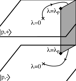
Figure 1: A path in parameter space interpolating smooothly between the vacua $|p,+\rangle$ and $|p,-\rangle$. The other vacua $|q,\pm\rangle$ for $q\not=p$ are not changed.

The physics underlying the smooth interpolation

$$|p,+\rangle\rightarrow|p,-\rangle$$ (19)

depicted in Figure 1 is best illustrated by looking at the domain walls. Consistently with the multivaluedness of the tension formulas (16,17,13), a D-brane is smoothly deformed into a solitonic brane,

$$(|p,+\rangle,|p+1,+\rangle)\rightarrow(|p,-\rangle,|p+1,+\rangle)\,,$$ (20)

and vice versa. In other words, the multivaluedness implies that there are several possible classical limits, some for which the tension scales as $N$, and others for which the tension scales as $N^{2}$. Obviously, at strong coupling, the distinction between D-branes and solitons does not make sense. This is particularly striking at the point $\lambda=\lambda_{p}$, for which

$$T_{(|p,+\rangle,|p+1,+\rangle)}(\lambda_{p}) =T_{(|p,-\rangle,|p+1,+\rangle)}(\lambda_{p})$$ (21)

$$\hskip-5.69046pt\mathop{\propto}_{N\rightarrow\infty}\sqrt{N}\sim 1/\sqrt{g_{\mathrm{s}}}\,.$$ (22)

We have discovered a new type of extended object in the theory at $\lambda=\lambda_{p}$, with a tension proportional to $\sqrt{N}\sim\sqrt{1/g_{\mathrm{s}}}$ [17]. Other fractional powers can be achieved by looking at more complicated branching points [17].

2.4 Quantum parameter space

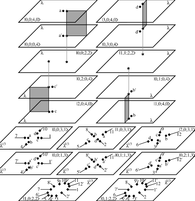
Figure 2: Sketch of the quantum parameter space $\mathcal{M}_{\mathrm{q}}$ for gauge group ${\rm U}(4)$. The sheets are parametrized by $\lambda$ or $\lambda^{1/3}$. The vacua for which $X$ has $N_{1}$ eigenvalues at zero and $N_{2}$ eigenvalues at $-m/g$ are denoted by $|k_{1},k_{2};N_{1},N_{2}\rangle$, with $k_{j}\in\mathbb{Z}_{N_{j}}$. The dots, squares and stars represent massless monopole points (at $\lambda=(4/5)e^{-ik\pi/2}$), branching points (at $\lambda^{1/3}=(3^{1/4}/2^{1/6})e^{-ik\pi/6}$), or both (at $\lambda=e^{-ik\pi/2}$), respectively. Due to the complexity of the diagram, we have not been able to represent explicitly all the identifications between sheets. It is understood that singularities and branch cuts with the same label are identified.

The physics discussed above is a basic consequence of a very general structure [17, 21, 22]. Let us consider the space, that we call the classical parameter space $\mathcal{M}_{\mathrm{cl}}$, whose points are labeled by the parameters of the gauge theory and by a given vacuum. The space $\mathcal{M}_{\mathrm{cl}}$ has many disconnected components, or sheets, each labeled by a vacuum. For example, in the theory (8), $\mathcal{M}_{\mathrm{cl}}$ has $\frac{1}{6}N(N^{2}+11)$ components parametrized by $\lambda$. In the full quantum theory, $W_{\rm low}$ is multivalued and the associated branch cuts glue some of the sheets together. The resulting space is called the quantum parameter space $\mathcal{M}_{\mathrm{q}}$ [17, 21]. The effective superpotential $W_{\rm low}$ is always a single-valued function on $\mathcal{M}_{\mathrm{q}}$.

For example, in the ${\rm U}(2)$ theory, $\mathcal{M}_{\mathrm{cl}}$ has five disconnected components corresponding to the four confining vacua $|0,+\rangle$, $|1,+\rangle$, $|0,-\rangle$, $|1,-\rangle$ and the Coulomb vacuum $|\mathrm{C}\rangle$. From the above discussion, we know that the sheets labeled by $|0,+\rangle$ and $|0,-\rangle$ on the one hand, and $|1,+\rangle$ and $|1,-\rangle$ on the other hand, are glued together. The Coulomb sheet cannot be smoothly connected to the other sheets, because it is in a different phase. However, there is a connection at points where monopoles become massless. The phase transition is triggered by the condensation of the massless monopoles through a standard Higgs mechanism in magnetic variables. Taking into account both the smooth interpolations through branch cuts and the phase transitions through massless monopole points, we get a fully connected quantum parameter space $\mathcal{M}_{\mathrm{q}}$ [17].

The ${\mathcal{N}}=1$ quantum parameter spaces are reminiscent of the ${\mathcal{N}}=2$ quantum moduli spaces, but there are important differences. The most notable is that motion on parameter space is not associated with a massless scalar, which makes the ${\mathcal{N}}=1$ models much more realistic. Moreover, the quantum corrections in ${\mathcal{N}}=1$ have even more drastic effects than in ${\mathcal{N}}=2$, since they change the topology of the classical space in addition to producing monopole singularities.

In all cases that have been studied so far, $\mathcal{M}_{\mathrm{q}}$ turns out to be fully connected. It is not known whether this is a general property. For example, the rather intricate case of ${\rm U}(4)$, with classically eighteen disconnected components, was worked out in [21]. The result is depicted in Figure 2. There are ten sheets in a confining phase and eight sheets in a Coulomb phase. The unbroken gauge group in the Coulomb phase can be either ${\rm U}(2)\times{\rm U}(2)$ (two vacua) or ${\rm U}(3)\times{\rm U}(1)$ (six vacua). To show that these eight sheets can be smoothly connected, we can study the analytic structure of $W_{\rm low}$ as already explained. It is often more convenient to work with the derivatives of $W_{\rm low}$, that yield the expectation values of various chiral operators. Remarquably, these vevs are the solutions of algebraic equations. In our case, it is natural to consider

$$u=-\frac{g}{m}\langle\mathop{\rm tr}\nolimits X\rangle\,.$$ (23)

The possible classical values of $u$ in the Coulomb phase are either one (three vacua with unbroken gauge group ${\rm U}(3)\times{\rm U}(1)$), two (the two ${\rm U}(2)\times{\rm U}(2)$ vacua) or three (three ${\rm U}(1)\times{\rm U}(3)$ vacua). This structure is manifest on the quantum equation satisfied by $u$ [21],

$$(u-1)^{3}(u-2)^{2}(u-3)^{3}+\frac{\lambda^{4}}{64}=0\,.$$ (24)

Varying $\lambda$, it is straightforward to show that the eight roots of (24) can be permuted, and thus that the eight Coulomb sheets are glued together by branch cuts. The full $\mathcal{M}_{\mathrm{q}}$ can be found by repeating this kind of argument and studying the possible phase transitions [21]. In [22], it was emphasized that the smooth interpolations can connect vacua with different patterns of gauge symmetry breaking. In our framework, this is a direct consequence of (24) for example.

2.5 Conclusions

Our main result was to show that D-branes can be smoothly deformed into solitonic branes and vice versa. We have also discovered new extended objects, with tensions scaling as fractional powers of the string coupling.

D-branes are simple in string theory but are hard to study in gauge theory. On the other hand, we have explained that solitonic branes can be quantized semiclassically in gauge theory. This provides a microscopic description of solitonic branes using gauge theories, which is the counterpart of the microscopic description of D-branes using open strings. Since a microscopic description of solitonic branes in string theory has remained elusive, this approach is probably worth pursuing.

3 Planar diagrams and Geometry

3.1 Calabi-Yau geometries

A famous non-compact Calabi-Yau geometry is the conifold $\mathcal{O}(-1)\oplus\mathcal{O}(-1)\rightarrow{\mathbb{P}}^{1}$. By wrapping $N$ D5 branes on the ${\mathbb{P}}^{1}$, we engineer the pure ${\mathcal{N}}=1$, ${\rm U}(N)$ gauge theory [23] with a Yang-Mills coupling

$$g^{2}_{\mathrm{YM}}\sim\frac{1}{\mathrm{vol}({\mathbb{P}}^{1})}\,\cdotp$$ (25)

To add adjoint chiral multiplets, we need to consider a more general local geometry

$$\mathcal{O}(-1+M)\oplus\mathcal{O}(-1-M)\rightarrow{\mathbb{P}}^{1}\,.$$ (26)

This space is Calabi-Yau because the first Chern class $2$ of the ${\mathbb{P}}^{1}$ and $-1-M-1+M=-2$ of the normal bundle compensate each other. It is not difficult to check, by direct analysis or by using the Riemann-Roch theorem, that the geometry (26) has a $M$-parameter family of holomorphic two-spheres. These $M$ parameters yield $M$ adjoint chiral multiplets $X_{i}$ in the world-volume gauge theory of D-branes wrapped on one of these two-spheres.

The existence of an $M$ dimensional continuous family of ${\mathbb{P}}^{1}$s implies that there is no superpotential for the $X_{i}$. To turn on a $W$, we generalize the geometry (26) to a new Calabi-Yau $\mathscr{M}$, covered by two coordinate patches $(z,w_{1},w_{2})$ and $(z^{\prime},w_{1}^{\prime},w_{2}^{\prime})$, and defined by the transition functions [18]

$$\mathscr{M}:\,\left\{\begin{matrix}\,\,z^{\prime}=1/z\hfill\ \\ w_{1}^{\prime}=z^{1-M}w_{1}\hfill\ \\ w_{2}^{\prime}=z^{1+M}w_{2}+\partial_{w}E(z,w_{1})\,.\hfill\ \end{matrix}\right.$$ (27)

When $E=0$, we find (26), but in general the perturbation $E$ is a non-zero function of two complex variables. It can be Laurent expanded in terms of entire functions (often polynomials) $E_{j}$ in the form

$$E(z,w)=\sum_{j=-\infty}^{+\infty}E_{j}(w)z^{j}\,.$$ (28)

From general arguments [24], it is known that perturbing the geometry (26) induces an obstruction to the space of versal deformations of the ${\mathbb{P}}^{1}$s. Holomorphic ${\mathbb{P}}^{1}$s can only exist at discrete values of the $X_{i}$ that are solutions of $M$ constraints (interestingly, the fact that the number of constraints is equal to the number of parameters is equivalent to the Calabi-Yau condition). In the case of (27), the constraints can be put in the form ${\rm d}W=0$ for a certain holomorphic function $W(X_{1},\ldots,X_{M})$. Turning on $E$ is the most general known perturbation having this property. Obviously, $W$ is the tree-level superpotential of the world volume gauge theory.

3.2 Superpotential

A formula to compute the superpotential in a variety of cases where branes are wrapped on two-cycles $\Sigma$ was given by Witten in [19],

$$W(\Sigma)=\int_{B}\Omega+\mathrm{constant}\,.$$ (29)

The chain $B$ is such that $\partial B=\Sigma-\Sigma_{0}$ for some fixed two-cycle $\Sigma_{0}$, and $\Omega$ is the holomorphic three-form. It is not difficult to check that the equations ${\rm d}W=0$ yield the correct conditions for $\Sigma$ to be holomorphic. In our case, $\Sigma$ is a two-sphere in $\mathscr{M}$, parametrized by the $X_{i}$, and computing the integral (29) yields $W(X_{1},\ldots,X_{M})$. This is perfectly good as long as we consider a single wrapped brane. When dealing with two or more branes, the $X_{i}$ are non-commuting matrices and (29) becomes ambiguous. The correct procedure is then to write directly the conditions for supersymmetry to be preserved. The $M$ equations for non-commuting variables so obtained can still be derived by extremizing a superpotential $W$ [18]

$$W=\frac{1}{2i\pi}\oint_{C_{0}}\!z^{-M-1}\mathop{\rm tr}\nolimits E\Bigl{(}z,\sum_{j=1}^{M}X_{j}z^{j-1}\Bigr{)}{\rm d}z\,.$$ (30)

The contour integral is over a small loop $C_{0}$ encircling the origin. In the commutative limit, (30) and (29) are of course equivalent.

For example, in the case $M=1$, (30) yields $W(X)=\mathop{\rm tr}\nolimits E_{1}(X)$. In the case $M=2$, we can consider an arbitrary superpotential $W(x,y)=\sum_{i,j\geq 0}a_{ij}x^{i}y^{j}$ in the commutative limit. The formula (30) gives the ordering prescription for any given monomial,

$$x^{i}y^{j}\mapsto\frac{i!j!}{(i+j)!}\oint_{C_{0}}\frac{{\rm d}z}{2i\pi}z^{-1-j}(X+Yz)^{i+j}\,.$$ (31)

This is the standard Weyl ordering.

The superpotential (30) includes as special cases all the previously engineered superpotentials for gauge theory with adjoints (see for example [25]). The associated multi-matrix integrals (2) are highly non-trivial and far beyond the grasp of ordinary matrix model techniques. Fortunately, we now have an entirely new point of view on the problem: the solution of the model amounts to finding the closed string background $\hat{\mathscr{M}}$ dual to the brane theory on $\mathscr{M}$. We shall now explore this strategy, by describing the two main steps required in the computation of the space $\hat{\mathscr{M}}$.

3.3 Blowing down

Holomorphic two-spheres in the geometry (27) are associated with the critical points of the superpotential (30). For a generic Morse critical point, the adjoint fields are massive and can be integrated out. This means that the normal bundle to the associated ${\mathbb{P}}^{1}$ is $\mathcal{O}(-1)\oplus\mathcal{O}(-1)$ as in the case of the pure ${\mathcal{N}}=1$ theory. More generally, if the corank of the Hessian of $W$ at the critical point is $r$, we expect the normal bundle to be $\mathcal{O}(-1+r)\oplus\mathcal{O}(-1-r)$, corresponding to a massless theory with $r$ adjoint multiplets. This was checked explicitly in the case $M=2$ in [18]. When $r\leq 2$, the low energy theory is asymptotically free, and we may expect that quantum mechanically the ${\mathbb{P}}^{1}$ shrinks to zero size. This heuristic RG argument is in beautiful agreement with a theorem by Laufer [26] that states that shrinkable spheres with normal bundle $\mathcal{O}(-1+r)\oplus\mathcal{O}(-1-r)$ must have $r=0,1$ or 2.

The blow down map

$$\pi:\ \mathscr{M}\rightarrow{\mathscr{M}}_{0}$$ (32)

is a birational isomorphism except on the ${\mathbb{P}}^{1}\subset\mathscr{M}$ that are mapped onto singular points of ${\mathscr{M}}_{0}$. Blowing down is a mathematically precise way to implement the heuristic picture of shrinking spheres. The calculation of the blow down map, for given $\mathscr{M}$, is a non-trivial problem. In the simplest cases, it amounts to finding four globally holomorphic functions $\pi_{i}(z,w_{1},w_{2})\in\mathbb{C}$ on $\mathscr{M}$ that maps the ${\mathbb{P}}^{1}$ onto points. Global holomorphicity is checked by using the transition functions (27). The four functions $\pi_{i}$ depend on three variables and satisfy in general an algebraic equation that defines the singular variety ${\mathscr{M}}_{0}$ as a hypersurface in $\mathbb{C}^{4}$. Several explicit examples can be found in [18].

In the geometric transition picture, the singular space ${\mathscr{M}}_{0}$ describes the classical $S\rightarrow 0$ matrix model (2), or equivalently the classical equations of motion

$${\rm d}W=\mathop{\rm tr}\nolimits{\rm d}V(X_{i})=0\,.$$ (33)

When the matrices $X_{i}$ are commuting (one dimensional representations), (33) reduces to a set of algebraic equations. By construction of the blow down map, these solutions are automatically associated with singular points in ${\mathscr{M}}_{0}$. More generally, the correspondence with the matrix model implies that the higher dimensional representations of (33) must also be associated with singular points on ${\mathscr{M}}_{0}$. This means that classical algebraic geometry must know about the non-commutative structure that emerges when considering D-branes.

Let us illustrate this point on a non-trivial example [18]. We consider the geometry

$$\mathscr{M}:\,\left\{\begin{matrix}\,\,z^{\prime}=1/z\hfill\ \\ w_{1}^{\prime}=z^{-1}w_{1}\hfill\ \\ w_{2}^{\prime}=z^{3}w_{2}+w_{1}^{2}-zG(w_{1}^{2}/z^{2})\\ &\hskip-85.35826pt-z^{2}F_{1}(w_{1}^{2})-z^{2}w_{1}F_{2}(w_{1}^{2})\,.\hfill\ \end{matrix}\right.$$ (34)

The corresponding superpotential is

$$W(X,Y)=\mathop{\rm tr}\nolimits\bigl{(}XY^{2}+A(X)+B(Y)\bigr{)}\,,$$ (35)

with $A^{\prime}(X)=-F_{1}(X^{2})-XF_{2}(X^{2})$ and $B^{\prime}(Y)=-G(Y^{2})$. The classical equations of motion are

$$\{X,Y\}=G(Y^{2})\,,\ Y^{2}=F_{1}(X^{2})+XF_{2}(X^{2})\,.$$ (36)

These equations can be analysed by noting that $X^{2}$ and $Y^{2}$ are Casimir operators. We find that there are $\max(\deg A^{\prime}+2,2\deg A^{\prime}\deg G)$ one dimensional irreducible representations and $[\frac{1}{2}(\deg A^{\prime}-1)]$ two dimensional irreducible representations (for which $X$ and $Y$ are linear combinations of Pauli matrices). On the other hand, the blow down map can be explicitly constructed [18] and the singular Calabi-Yau is found to be

$$\hskip-7.11317pt{\mathscr{M}}_{0}:\,x_{2}\bigl{[}(x_{2}-F_{1}(x_{1}))^{2}-x_{1}F_{2}^{2}(x_{1})\bigr{]}=x_{4}^{2}-x_{1}x_{3}^{2}\\ -G(x_{2})\bigl{[}(x_{2}-F_{1}(x_{1}))x_{3}+x_{4}F_{2}(x_{1})\bigr{]}\,.$$ (37)

It is not difficult to check that ${\mathscr{M}}_{0}$ has singular points for both one and two dimensional representations.

The fact that the full set of solutions of matrix equations can be encoded in a set of algebraic equations describing the singularities of a Calabi-Yau is a remarkable feature. In all the cases that have been worked out, the solutions to the matrix equations can be characterized by a set of Casimir operators. These Casimirs turn out to be associated with some coordinates on ${\mathscr{M}_{0}}$. The special values of the Casimirs labeling the solutions then match the values of the coordinates at the singular points. For example, in the case (37), the coordinate $x_{1}$ is associated with the Casimir $X^{2}$ and the coordinate $x_{2}$ with the Casimir $Y^{2}$.

3.4 Deforming

The full $S\not=0$ matrix model (2) is described by a deformed non-singular geometry $\hat{\mathscr{M}}$ whose equation is obtained from the equation for ${\mathscr{M}}_{0}$ by adding certain monomials $\sum c_{abcd}x_{1}^{a}x_{2}^{b}x_{3}^{c}x_{4}^{d}$. The allowed monomials must be such that the divergences in the period integrals $\oint\Omega$ of the holomorphic three-form over non-compact cycles are either $S$-independent of linear in $S$ and logarithmic. This condition is the mathematical counterpart of the renormalization properties of the ${\mathcal{N}}=1$ Yang-Mills theories. After implementing this constraint, and taking into account possible coordinate redefinitions, we obtain a certain number ${\mathscr{N}}_{\mathrm{geo}}$ of independent and freely adjustable coefficients $c_{abcd}$ that parametrize the geometry $\hat{\mathscr{M}}$.

The parameters $c_{abcd}$ should not be confused with the parameters in the superpotential or equivalently in the original geometry (27). They have a very natural interpretation in terms of the matrix model. The matrix integrals (2) are defined by summing over planar Feynman diagrams. The Feynman rules are themselves defined by expanding around a particular solution of the classical equations of motion. The most general classical solution is the direct sum of the irreducible representations of (33), and is thus characterized by parameters, called filling fractions, giving the fraction of eigenvalues in given irreducible representations. The number ${\mathscr{N}}_{\mathrm{alg}}$ of filling fractions that need to be specified is thus equal to the number of irreducible representations of (33). Consistency requires that there should exist a one-to-one mapping between the filling fractions and the $c_{abcd}$, and thus that

$${\mathscr{N}}_{\mathrm{geo}}={\mathscr{N}}_{\mathrm{alg}}\,.$$ (38)

This is a profound equality relating classical geometry and non-commutative algebra: the left-hand side is computed by studying the “renormalizable” deformation of a certain singular Calabi-Yau space, and the right-hand side is computed by working out the representation theory of a certain matrix algebra. This correspondence follows rather straightforwardly from the physical picture, but remains to be understood at a deeper mathematical level. It was checked explicitly in a variety of non-trivial examples in [18]. For example, in the theory (34,35,37), detailed calculations show that

$${\mathscr{N}}_{\mathrm{alg}}=\max\bigl{(}\deg A^{\prime}+2,2\deg A^{\prime}\deg G\bigr{)}\\ +\bigl{[}(\deg A^{\prime}-1)/2\bigr{]}={\mathscr{N}}_{\mathrm{geo}}$$ (39)

as expected.

3.5 The solution

In the case of the one-matrix model $W=\mathop{\rm tr}\nolimits V(X)$, it is well-known that the deformed geometry takes the simple form

$$\hat{\mathscr{M}}:\ x_{4}^{2}=x_{3}^{2}+x_{2}^{2}-V^{\prime}(x_{1})^{2}+S\Delta(x_{1})\,,$$ (40)

where $\Delta$ is a polynomial of degree $\deg V^{\prime}-1$ describing the deformation of ${\mathscr{M}}_{0}$ (in this case it is obvious that $\mathscr{N}_{\mathrm{alg}}=\deg V^{\prime}$; it is also straightforward to show that $\mathscr{N}_{\mathrm{geo}}=\deg V^{\prime}$ by computing the periods $\oint\Omega$). It is useful to think about (40) as a fibration over a base parametrized by $x_{1}$. The fiber $F_{x_{1}}$ at $x_{1}$ is the simplest ALE space $\mathbb{C}^{2}/\mathbb{Z}_{2}$, and contains a single holomorphic two-sphere $S^{2}$. The discontinuity of the resolvent

$$g^{X}(x)=S\Bigl{\langle}\frac{\mathop{\rm tr}\nolimits}{n}\frac{1}{x-X}\Bigr{\rangle}$$ (41)

across its branch cuts is then simply given by

$$g^{X}(x+i\epsilon)-g^{X}(x-i\epsilon)=\int_{S^{2}\subset F_{x}}\mathrm{i}_{X}\Omega\,,$$ (42)

where $\mathrm{i}_{X}$ denotes the interior product with respect to the vector field $\partial/\partial x_{1}$.

More general multi-matrix models can always be reduced to one matrix models with a complicated effective potential after integration over all but one matrix. This shows that the structure just described is still relevant, but the fibers $F_{x}$ are typically much more complicated than $\mathbb{C}^{2}/\mathbb{Z}_{2}$, and contains many two-spheres (as a consequence of the multivaluedness of the effective potential). The basic formula (42) is still valid [18] and can be used to find explicitly the resolvents of the various matrices of multi-matrix models. For example, in the case of (35), it is shown with this method that $g^{X}$ satisfies a degree $\max(3,2+2\deg G)$ algebraic equation and that $g^{Y}$ lies at the intersection of $d$ quadrics in a $d$-dimensional auxiliary space [18]. It appears to be very difficult to obtain these results using standard matrix model technology. Nevertheless, in the special case where $G$ is a constant, the loop equations can be solved [18] and full agreement is found with the geometry.

3.6 Conclusions

We have a rich interplay between algebraic geometry and matrix models, that suggests many non-trivial results. There are many open problems: can we understand the special properties of the matrix models with potentials (30) (irreducible representations of the classical equations of motion, loop equations, etc…)?; does the potential (30) describes the most general matrix model that can be engineered in string theory?; can we give a direct mathematical proof of the relation between the singularity structure of ${\mathscr{M}}_{0}$ and the representations of (33)?; and so on. The most important question is probably to understand whether the blow down map for the geometry (27) always exists. This is a hard mathematical problem [27]. If it does, and if we can find an algorithm to compute it, then we have solved a huge class of multi-matrix models (30). If it does not, then the picture of geometric transitions cannot deal with our examples in general, with fundamental consequences for our understanding of the structure of ${\mathcal{N}}=1$ vacua in string theory.

4 Homework

4.1 Exercices

a) Prove or disprove that the ${\mathcal{N}}=1$ quantum parameter spaces are always connected.

b) Describe the correct microscopic description of solitonic branes using gauge theory.

4.2 Problem

Consider the geometry (27).

i) Find the blow down geometry. Compare with the algebra ${\rm d}W=0$ where $W$ is given by (30).

ii) Find the deformed geometry. Check (38).

iii) Compute the resolvents from the geometry. Compare with the loop equations.

References

- [1] C. Montonen and D. Olive, Phys. Lett. B 72 (1977) 117.
- [2] A. Sen, Phys. Lett. B 329 (1994) 217, hep-th/9402032.
- [3] N. Seiberg and E. Witten, Nucl. Phys. B 426 (1994) 19, erratum B 430 (1994) 485, hep-th/9407087.
- [4] A. Klemm, W. Lerche, S. Yankielowicz and S. Theisen, Phys. Lett. B 344 (1995) 169, hep-th/9411048.
- [5] R.Y. Donagi, Seiberg-Witten integrable systems, alg-geom/9705010.
-
[6]
A. Klemm, W. Lerche, P. Mayr, C. Vafa and N. Warner,
Nucl. Phys. B 477 (1996) 746, hep-th/9604034,
S. Katz, A. Klemm and C. Vafa, Nucl. Phys. B 497 (1997) 173, hep-th/9609239. - [7] A. Giveon and D. Kutasov, Rev. Mod. Phys. 71 (1999) 983, hep-th/9802067.
- [8] N. Seiberg and E. Witten, Nucl. Phys. B 431 (1994) 484, hep-th/9408099.
-
[9]
A. Bilal, in Quantum fields and quantum
space-time, Cargèse 1996, page 21, hep-th/9601007,
L. Alvarez-Gaumé and S.F. Hassan, Fortsch. Phys. 45 (1997) 159, hep-th/9701069. - [10] K. Intriligator and N. Seiberg, Lectures on supersymmetric gauge theories and electric-magnetic duality,, Nucl. Phys. Proc. Suppl. 55 (1997) 1, hep-th/9509066.
-
[11]
F. Ferrari and A. Bilal, Nucl. Phys. B 469 (1996) 387,
hep-th/9602082,
F. Ferrari, Nucl. Phys. B 516 (1998) 175, hep-th/9706145. - [12] O. Aharony, S.S. Gubser, J.M. Maldacena, H. Ooguri and Y. Oz, Phys. Rep. 323 (2000) 183, hep-th/9905111.
- [13] F. Ferrari, Lectures on Supersymmetric Gauge Theories, Matrix Models and Geometric Transitions, to appear, NEIP-03-003, LPTENS-04/43, hep-th/0411nnn.
-
[14]
I. Antoniadis, E. Gava, K.S. Narain and T.R. Taylor,
Nucl. Phys. B 413 (1994) 162, hep-th/9307158,
M. Bershadsky, S. Cecotti, H. Ooguri and C. Vafa, Comm. Math. Phys. 165 (1994) 311, hep-th/9309140. -
[15]
R. Gopakumar and C. Vafa, Adv. Theor. Math. Phys. 3 (1999) 1415,
hep-th/9811131,
C. Vafa, J. Math. Phys. 42 (2001) 2798, hep-th/0008142,
F. Cachazo, K. Intriligator and C. Vafa, Nucl. Phys. B 603 (2001) 3, hep-th/0103067. - [16] R. Dijkgraaf and C. Vafa, hep-th/0208048.
- [17] F. Ferrari, Phys. Rev. D 67 (2003) 85013, hep-th/0211069.
- [18] F. Ferrari, Adv. Theor. Math. Phys. 7 (2003) 619, hep-th/0309151.
- [19] E. Witten, Nucl. Phys. B 507 (1997) 658, hep-th/9706109.
- [20] F. Ferrari, Nucl. Phys. B 648 (2002) 68, hep-th/0210135.
- [21] F. Ferrari, Phys. Lett. B 557 (2003) 290, hep-th/0301157.
- [22] F. Cachazo, N. Seiberg and E. Witten, J. High Energy Phys. 02 (2003) 042, hep-th/0301006.
- [23] J.M. Maldacena and C. Nuñez, Phys. Rev. Lett. 86 (2001) 588, hep-th/0008001.
- [24] M. Namba, Tôhoku Math. J. 24 (1972) 581.
- [25] F. Cachazo, S. Katz and C. Vafa, hep-th/0108120.
- [26] H.B. Laufer, Ann. of Math. Stud. 100 (1981) 261.
- [27] J. Kollár, private communication.