Abstract

In ten dimensional type II superstring, all perturbative massive states are unstable, typically with a short lifetime compared to the string scale. We find that the lifetime of the average string state of mass $M$ has the asymptotic form $\bar{\cal T}\leq{\rm const.}g_{s}^{-2}\ M^{-1}$. The most stable string state seems to be a certain state with high angular momentum which can be classically viewed as a circular string rotating in several planes (“the rotating ring”), predominantly decaying by radiating soft massless NS-NS particles, with a lifetime ${\cal T}=c_{0}g_{s}^{-2}M^{5}$. Remarkably, the dominant channel is the decay into a similar rotating ring state of smaller mass. The total lifetime to shrink to zero size is $\sim M^{7}$. In the presence of D branes, decay channels involving open strings in the final state are exponentially suppressed, so the lifetime is still proportional to $M^{5}$, except for a D brane at a special angle or flux. For large mass, the spectrum for massless emission exhibits qualitative features typical of a thermal spectrum, such as a maximum and an exponential tail. We also discuss the decay properties of rotating rings in the case of compact dimensions.

UB-ECM-PF-04/30 SISSA-72/2004/EP hep-th/0410152

Search for the most stable massive state
in superstring theory

Diego Chialva ^a,b , Roberto Iengo ^a,b and Jorge G. Russo ^c

^a International School for Advanced Studies (SISSA)
Via Beirut 2-4, I-34013 Trieste, Italy

^b INFN, Sezione di Trieste

^c Institució Catalana de Recerca i Estudis Avançats (ICREA),

Departament ECM, Facultat de Física, Universitat de Barcelona, Spain

chialva@sissa.it, iengo@he.sissa.it, jrusso@ecm.ub.es

1 Introduction

Understanding the decay properties of massive string states may uncover new aspects of string theory dynamics, and it may also have direct implications in cosmology (see e.g. [1, 2, 3, 4]). According to their decay properties, the quantum states of the type II string spectrum can be divided into two classes:

i) Those for which the dominant decay channel is by massless emission.

ii) Those for which the dominant decay channel is by emission of massive particles.

In [5] we argued that massless emission is the dominant channel whenever the quantum state corresponds to large closed strings which cannot break during the evolution. An example of this is the rotating ring: the string is circular, and there is never a contact between two points of the string. For these class i) string states, the decay channels into massive states are exponentially suppressed, we indeed find $\Gamma_{\rm massive}=O(e^{-cM^{2}})$, where the value of $c$ depends on the specific state. An example of a class ii) state is the folded closed string corresponding to the quantum state with maximum angular momentum: the points of the string are always in contact with the other side so the string can break at any moment. This picture was confirmed in detail by the calculations of [5]. With this line of argument, in [5] we have identified a one-parameter family of long-lived string states.

For the class i) quantum states, the lifetime is given by ${\cal T^{\rm(i)}}=\Gamma_{\rm massless}^{-1}$, while for the class ii) quantum states, the decay rate for massless emission $\Gamma_{\rm massless}$ puts an upper bound on the lifetime, i.e. ${\cal T^{\rm(ii)}}\leq\Gamma_{\rm massless}^{-1}$. In this paper we will concentrate on the calculation of $\Gamma_{\rm massless}$, first finding a simple general formula, and then carrying out the analytic calculation in detail for the case of the rotating ring. The analytic calculation confirms the lifetime ${\cal T}_{\rm ring}={c_{0}\over g_{s}^{2}}M^{5}$, in ten uncompact spacetime dimensions, obtained in [5] by numerical evaluation of the imaginary part of the one-loop correction to the two-point function (here we also determine $c_{0}$). Further, we show that for large $M$ the decay occurs by the emission of massless quanta of feeble energy $\omega\sim 1/M$ and that the ring final state is just the same as the initial one, only slightly shrunk to conserve energy. Moreover, we show that for large mass a classical computation gives exactly the same results as the quantum one. That is, the rotating ring slowly radiates as a classical antenna (section 3.3). In section 4 we show that the rotating ring has the same lifetime ${\cal T}_{\rm ring}={c_{0}\over g_{s}^{2}}M^{5}$ in the presence of generic configurations of D branes. This is due to the fact that the decay into open strings is exponentially suppressed, except for a D brane at a special angle.

The case of compact dimensions is discussed in section 5. The decay properties of the ring then depend on the ring configuration, in particular, on whether the ring lies on compact or uncompact dimensions. For configurations where decay into winding modes is suppressed, the lifetime of the rotating ring is ${\cal T}={\rm const.}g_{s}^{-2}\ M^{d-4}$, where $d$ is the number of uncompact spatial dimensions, while the total lifetime for the ring to shrink to microscopic size is ${\cal T}_{\rm tot}={\rm const.}g_{s}^{-2}\ M^{d-2}$.

In section 6, we compute $\bar{\Gamma}_{\rm massless}$ representing the average over all initial states of given mass $M$ (following the similar calculation carried out in [9] for the bosonic string).

Some earlier discussions of decays of massive string states can be found in [6, 7, 8]. The average decay rate by massless emission in bosonic string theory is given in [9] and a study of massive emission from an average string state is in [10] (averages involving two massless vertices were discussed in [11]). The classical breaking of the string and the correspondence with the quantum calculation is discussed in [12]. A numerical study of the decay of the rotating ring in compactified dimensions from the one-loop two-point function is in [13].

2 General formula for decay rates

The total decay amplitude of a state $|\Phi_{0}\rangle$ of mass $M$ for emission of a massless (fermion or boson) particle $(\omega,\vec{k})$ represented by a vertex operator $V$ is given by

$$\Gamma(\omega)={g_{s}^{2}\over 8M}\int{d\Omega^{d-1}d\omega\ \omega^{d-2}\over(2\pi)^{d-1}E^{\prime}}\delta(M-E^{\prime}-\omega)\ \sigma_{R}\ \sigma_{L}\ ={g_{s}^{2}\over 8(2\pi)^{d-1}}{\omega^{d-2}\over M^{2}}\int d\Omega^{d-1}\ \sigma_{R}\ \sigma_{L}\ ,$$ (2.1)

where $d$ is the number of spatial dimensions and

$$\sigma_{R}=\sum_{\Phi_{N^{\prime}}}\langle\Phi_{0}|V_{R}(k,1)^{\dagger}|\Phi_{N^{\prime}}\rangle\langle\Phi_{N^{\prime}}|V_{R}(k,1)|\Phi_{0}\rangle\ ,$$ (2.2)

and a similar expression for $\sigma_{L}$. The sum goes over all states with mass $M^{\prime}=\sqrt{N^{\prime}}$, with energy $E^{\prime}=\sqrt{{M^{\prime}}^{2}+\omega^{2}}$, and (in units $\alpha^{\prime}=4$)

$$\omega={M^{2}-{M^{\prime}}^{2}\over 2M}={N_{0}\over 2\sqrt{N}}\ ,\ \ \ M^{2}=N\ ,\ \ N_{0}\equiv N-N^{\prime}\ .$$

Introducing a projector onto states of level $N^{\prime}$,

$$\sum_{\Phi_{N^{\prime}}}|\Phi_{N^{\prime}}\rangle\langle\Phi_{N^{\prime}}|=\oint{dz\over z}\ z^{\hat{N}_{R}-{N^{\prime}}}\ ,$$ (2.3)

the decay amplitude can be computed as

$$\sigma_{R}=\oint{dz\over z}\ z^{-{N^{\prime}}}\langle\Phi_{0}|V_{R}(k,1)^{\dagger}z^{\hat{N}_{R}}V_{R}(k,1)|\Phi_{0}\rangle\ .$$ (2.4)

By using the standard commutators

$$[a,a^{\dagger}]=1\ ,\ \ \ \{\psi,\psi^{\dagger}\}=1\ ,\ \ \ z^{na^{\dagger}a}e^{a}=e^{a/z^{n}}z^{na^{\dagger}a}\ ,\ \ \ z^{r\psi^{\dagger}\psi}e^{\psi}=e^{\psi/z^{r}}z^{r\psi^{\dagger}\psi}\ ,$$

one can write

$$z^{\hat{N}_{R}}V_{R}(k,1)=V_{R}(k,z)z^{\hat{N}_{R}}\ .$$ (2.5)

Thus

$$\sigma_{R}=\oint{dz\over z}\ z^{N-{N^{\prime}}}\langle\Phi_{0}|V_{R}(k,1)^{\dagger}V_{R}(k,z)|\Phi_{0}\rangle\ .$$ (2.6)

For massless NS-NS emission, one considers the vertex operator $V=g_{s}\ V_{L}V_{R}$, with

$$V_{R}=(\xi.\partial X_{R}+i\ \xi.\psi_{R}\ k.\psi_{R})\ e^{ik.X_{R}},\ \ V_{L}=(\tilde{\xi}.\bar{\partial}X_{L}+i\ \tilde{\xi}.\psi_{L}\ k.\psi_{L})\ e^{ik.X_{L}},$$ (2.7)

$$\xi.k=\tilde{\xi}.k=0\ ,\ \ \ \ k^{2}=0\ .$$ (2.8)

We will work in the gauge where $\xi_{0}=\tilde{\xi}_{0}=0$. Equations (2.1), (2.6), allow to compute the decay rate of any quantum state of the string spectrum by computing a matrix element involving standard free/creation annihilation operators. In the next section we carry out this calculation for the rotating ring. The calculation can also be carried out for other states in a straightforward way.

.

3 The rotating ring

3.1 Decay rate

We now consider the following state

$$|\Phi_{0}\rangle={{b^{\dagger}}^{N}\over\sqrt{N!}}\psi_{-1/2}^{Z_{1}}|0\rangle_{R}\ \times\ {({\tilde{c}}^{\dagger})^{N}\over\sqrt{N!}}\tilde{\psi}_{-1/2}^{Z_{2}}|0\rangle_{L}\ ,$$ (3.1)

where we define $b^{\dagger}\equiv b_{1+}^{\dagger}={\alpha_{-1}^{X_{1}}+i\alpha_{-1}^{X_{2}}\over\sqrt{2}}$, $\tilde{c}^{\dagger}\equiv\tilde{c}_{1+}^{\dagger}={\tilde{\alpha}_{-1}^{X_{3}}+i\tilde{\alpha}_{-1}^{X_{4}}\over\sqrt{2}}$ (see appendix A for notation). The operator $b^{\dagger}$ ($\tilde{c}^{\dagger}$) adds one unit of Right (Left) angular momentum in the plane 12 (34). This state has

$$N_{R}=N_{L}=N\ ,\ \ \ \ \alpha^{\prime}M^{2}=4N\ ,\ \ \$$ (3.2)

$$J_{12R}=N,\ \ \ J_{12L}=0,\ \ \ \ J_{34R}=0,\ \ \ J_{34L}=N,$$ (3.3)

so that $J_{12}=J_{34}=N$. The classical string soliton solution with the same values of $J_{12R},J_{12L}$, $J_{34R},J_{34L}$ is as follows

$$Z_{1}=L\ e^{-i(\sigma-\tau)}\ ,\ \ \ \ Z_{2}=L\ e^{i(\sigma+\tau)}\ ,\ \ \ \ \ L=\sqrt{\alpha^{\prime}N\over 2}\ ,$$ (3.4)

$$X_{0}=2\sqrt{2}L\ \tau\ ,\ \ \ \ \ \sigma\in[0,2\pi)\ .$$

It describes a circular string rotating around its axes in two orthogonal planes. One can also write similar rotating ring solutions (and the corresponding quantum states) with rotation in different planes.

The lifetime of this state was studied in [5] by a numerical evaluation of the imaginary part of the one-loop two point amplitude. It was shown that it goes like ${\cal T}\sim M^{5}$, and that the dominant decay channel is massless emission. Other decay channels representing decay into two massive particles are suppressed exponentially for large mass of the initial state, i.e. the decay rate for these massive channels is $\Gamma\sim\exp(-cM^{2})$. Thus in the large mass limit, the only contribution which is not exponentially suppressed is decay by emission of a single massless particle (multiple massless particle emission is suppressed by extra factors of $g_{s}^{2}$). This can be computed analytically by using the operator approach, as explained in section 2.

Let us start considering emission of a NS-NS massless particle. It is convenient to introduce complex notation

$$\kappa={1\over\sqrt{2}}(k_{1}+ik_{2})\ ,\ \ \ \ \tilde{\kappa}={1\over\sqrt{2}}(k_{3}+ik_{4})\ ,$$ (3.5)

$$\varepsilon={1\over\sqrt{2}}(\xi_{1}+i\xi_{2})\ ,\ \ \ \tilde{\varepsilon}={1\over\sqrt{2}}(\tilde{\xi}_{3}+i\tilde{\xi}_{4})\ .$$ (3.6)

Now consider the computation of $\sigma_{R}$ (2.6),

$$\sigma_{R}=\oint{dz\over z}\ z^{N_{0}}\langle 0|{b^{N}\over\sqrt{N!}}\psi_{1/2}^{\bar{Z}}V_{R}(k,1)^{\dagger}V_{R}(k,z){{b^{\dagger}}^{N}\over\sqrt{N!}}\psi_{-1/2}^{Z}|0\rangle\ ,$$ (3.7)

with $N_{0}\equiv N-N^{\prime}$. The product $V_{R}(1)^{\dagger}V_{R}(z)$ gives rise to five contributions,

$$\sigma_{R}=\sigma_{1}+\sigma_{2}+\sigma_{3}+\sigma_{4}+\sigma_{5}\ ,$$ (3.8)

with

$$\sigma_{1}=-{1\over N!}\oint{dz\over z}\ z^{N_{0}}\langle 0|b^{N}:e^{-ik.X(1)}e^{ik.X(z)}\xi.\partial X(1)\xi.\partial X(z):{b^{\dagger}}^{N}|0\rangle\ ,$$ (3.9)

where we have used $\langle 0|\psi_{1\over 2}^{\bar{Z}}\psi_{-{1\over 2}}^{Z}|0\rangle=1$, and $\sigma_{2},...,\sigma_{5}$ are given in appendix B.

For large $N$, $\sigma_{1}$ turns out to be the dominant contribution, while $\sigma_{2},...,\sigma_{5}$ are suppressed by inverse powers of $N$ (see Section 3.2).

Using the algebra of creation/annihilation operators, we obtain $\sigma_{1}=\sigma_{1}^{(I)}+\sigma_{1}^{(II)}$, with

$$\sigma_{1}^{(I)}=\big{(}\bar{\varepsilon}^{2}\kappa^{2}+\varepsilon^{2}\bar{\kappa}^{2}\big{)}\oint{dz\over z^{2}}z^{N_{0}}\sum_{m=0}^{N-2}{4\ N!(2\kappa\bar{\kappa})^{m}\over m!(m+2)!(N-m-2)!}{(1-z)^{2m+2}\over z^{m}}\ ,$$

$$\sigma_{1}^{(II)}=2\bar{\varepsilon}\varepsilon\oint{dz\over z}z^{N_{0}}\big{(}z+z^{-1}\big{)}\sum_{m=0}^{N-1}{N!(2\kappa\bar{\kappa})^{m}\over m!^{2}(N-m-1)!}{(1-z)^{2m}\over z^{m}}\ .$$

Now we expand the binomial $(1-z)^{r}$ and perform the integrals in $z$ around a small contour near $z=0$. We find

$$\sigma_{1}^{(I)}=4(2\kappa\bar{\kappa})^{N_{0}-1}\big{(}\bar{\varepsilon}^{2}\kappa^{2}+\varepsilon^{2}\bar{\kappa}^{2}\big{)}\sum_{r=0}^{N-N_{0}-1}c_{I}(r)\ (-2\kappa\bar{\kappa})^{r}\ ,$$ (3.10)

$$\sigma_{1}^{(II)}=4(2\kappa\bar{\kappa})^{N_{0}-1}\bar{\varepsilon}\varepsilon\sum_{r=0}^{N-N_{0}}c_{II}(r)\ (-2\kappa\bar{\kappa})^{r}\ ,$$ (3.11)

where

$$c_{I}(r)={N!(2r+2N_{0})!\over r!(N-N_{0}-1-r)!(r+2N_{0})!(r+N_{0}-1)!(r+N_{0}+1)!}\ ,$$ (3.12)

$$c_{II}(r)={N!(2r+2N_{0}-2)![r^{2}+(r+N_{0})(2N_{0}-1)]\over r!(N-N_{0}-r)!(r+2N_{0})!(r+N_{0}-1)!^{2}}\ .$$ (3.13)

Next, we sum over polarizations, using the relations given in appendix A. We obtain

$$\sigma_{1}^{(I)}=-2\left({N_{0}^{2}v^{2}\over 4N}\right)^{N_{0}}\ v^{2}\sum_{r=0}^{N-N_{0}-1}c_{I}(r)\ \left(-{N_{0}^{2}v^{2}\over 4N}\right)^{r}\ ,$$ (3.14)

$$\sigma_{1}^{(II)}=4\left({N_{0}^{2}v^{2}\over 4N}\right)^{N_{0}-1}(1-{v^{2}\over 2})\sum_{r=0}^{N-N_{0}}c_{II}(r)\ \ \left(-{N_{0}^{2}v^{2}\over 4N}\right)^{r}\ .$$ (3.15)

where $v^{2}\equiv\sin^{2}\theta\cos^{2}\alpha\cos^{2}\beta$. The Left contributions are similar, changing $\kappa,\bar{\kappa}$ by $\tilde{\kappa},\bar{\tilde{\kappa}}$ and $\xi^{\mu}$ by $\tilde{\xi}^{\mu}$, with $2\tilde{\kappa}^{2}={N_{0}^{2}\over 4N}\ e^{2i\psi}\sin^{2}\theta\cos^{2}\alpha\sin^{2}\beta$.

Now we consider the product $\sigma_{T}=\sigma_{L}\times\sigma_{R}$ and perform the integral over the angular part. Defining

$$I(r,s)=\int d^{8}\Omega(\sin\theta\cos\alpha)^{2r+2s}(\cos\beta)^{2r}(\sin\beta)^{2s}={(2\pi)^{4}\sqrt{\pi}\ r!s!\over 8~{}\Gamma({9\over 2}+r+s)}\ ,$$ (3.16)

we find

$$\int d^{8}\Omega\ \sigma_{T}=\Sigma_{11}+\Sigma_{22}+2\Sigma_{12}\ ,$$ (3.17)

with

$$\Sigma_{11}=4\left({N_{0}^{2}\over 4N}\right)^{2N_{0}}\ \sum_{r,s=0}^{N-N_{0}-1}\left(-{N_{0}^{2}\over 4N}\right)^{r+s}c_{I}(r)c_{I}(s)I(r+N_{0}+1,s+N_{0}+1)\ ,$$ (3.18)

$$\Sigma_{22}=16\left({N_{0}^{2}\over 4N}\right)^{2N_{0}-2}\ \sum_{r,s=0}^{N-N_{0}}\left(-{N_{0}^{2}\over 4N}\right)^{r+s}c_{II}(r)c_{II}(s)J(r+N_{0}-1,s+N_{0}-1)\ ,$$ (3.19)

$$\Sigma_{12}=-8\left({N_{0}^{2}\over 4N}\right)^{2N_{0}-1}\ \sum_{r=0}^{N-N_{0}-1}\sum_{s=0}^{N-N_{0}}\left(-{N_{0}^{2}\over 4N}\right)^{r+s}c_{I}(r)c_{II}(s)K(r+N_{0}-1,s+N_{0}-1)\ ,$$ (3.20)

$$J(m,n)\equiv I(m,n)-{1\over 2}I(m+1,n)-{1\over 2}I(m,n+1)+{1\over 4}I(m+1,n+1)\ ,$$

$$K(m,n)\equiv I(m+2,n)-{1\over 2}I(m+2,n+1)\ .$$

Thus the total decay amplitude for emission of a massless NS-NS particle from the rotating ring is given by

$$\Gamma(\omega)={g_{s}^{2}\over 8(2\pi)^{8}}{\omega^{7}\over M^{2}}\big{(}\Sigma_{11}+\Sigma_{22}+2\Sigma_{12}\big{)}\ .$$ (3.21)

Using $\omega=N_{0}/(2M),\,m+\sqrt{N}$, this can be written as

$$\Gamma(\omega)=g_{s}^{2}\ N^{-{5\over 2}}\ f(N_{0},N)\ ,$$ (3.22)

with

$$f(N_{0},N)={g_{s}^{2}\over 2^{10}(2\pi)^{8}}{N_{0}^{7}\over N^{2}}\big{(}\Sigma_{11}+\Sigma_{22}+2\Sigma_{12}\big{)}\ .$$ (3.23)

This function $f(N_{0},N)$ becomes independent of $N$ for large $N$. This is due to the fact that the main contributions arise for finite $N_{0}$ for any $N$ (see sect. 3.4). In fact, it has a maximum at $N_{0}=3$ irrespective of the value of $N$ (provided $N>9$). For large $N$, one can then use the Stirling approximation to write, in $c_{I}(r),\ c_{II}(r)$,

$${N!\over(N-m)!}\sim N^{m}\ .$$ (3.24)

Then the $N$ dependence in $f(N_{0},N)$ fully cancels out. Indeed, from $c_{I}(r)c_{I}(s)$ one gets a power $N^{2N_{0}+r+s+2}$ which cancels all powers of $N$ in $\Sigma_{11}$, and similarly for $\Sigma_{12}$ and $\Sigma_{22}$. Thus we can replace $f(N_{0},N)$ by $\bar{f}(N_{0})=f(N_{0},\infty)$ so that the large $N$ result is

$$\Gamma(N_{0})=g_{s}^{2}\ M^{-{5}}\ \bar{f}(N_{0})\ .$$ (3.25)

The total decay rate can now be computed by summing over all $N_{0}$ from 1 to $N$:

$$\Gamma_{\rm massless}=g_{s}^{2}\ M^{-{5}}\sum_{N_{0}=1}^{N}f(N_{0},N)\cong g_{s}^{2}\ M^{-{5}}\sum_{N_{0}=1}^{\infty}\bar{f}(N_{0})\ ,$$ (3.26)

In the next section, we show that massless fermion emission and emission of massless RR states are suppressed by factors $1/N$ and $1/N^{2}$ respectively, so $\Gamma_{\rm massless}$ represents the complete decay rate modulo $1/N$ corrections. Thus, for large initial mass, the lifetime of the rotating ring is given by

$${\cal T}_{\rm ring}=\Gamma^{-1}_{\rm massless}=c_{0}g_{s}^{-2}\ M^{{5}}\ ,\ \ \ \ c_{0}\equiv\sum_{N_{0}=1}^{\infty}\bar{f}(N_{0})\cong{8(2\pi)^{8}\over 12.5}\ .$$ (3.27)

This exactly reproduces the result of [5] obtained by computing the imaginary part of the one-loop two-point function (modulo the numerical coefficient $c_{0}$ which had not been determined in [5]).

3.2 Dominant decay channel

The large $N$ behavior of the various terms giving the massless (radiation) emission rate can be understood in brief by the following sample computation.

Consider the term $\langle\Phi_{N}^{\rm ring}|\hat{O}\{X\}|\Phi_{N}^{\rm ring}\rangle$, $\hat{O}\{X\}\equiv:\xi.\partial X(1)\xi.\partial X(z)e^{-ik\cdot X(1)+ik\cdot X(z)}:$ , appearing in the Right factor. We can restrict the full operator $\hat{O}\{X\}$ to the part containing $b,b^{{\dagger}}$, as only this part gives a contribution. Ignoring the factors $\xi$ and the dependence on $z$, we have

$$\langle\Phi_{N}^{\rm ring}|\hat{O}\{X\}|\Phi_{N}^{\rm ring}\rangle\sim\langle 0|{b^{N}\over\sqrt{N!}}b^{\dagger}e^{-\sqrt{2}\bar{\kappa}b^{\dagger}}b\ e^{\sqrt{2}\kappa b}~{}{b^{\dagger N}\over\sqrt{N!}}|0\rangle=\sum_{m=0}^{N-1}{N!(-2\kappa\bar{\kappa})^{m}\over m!^{2}(N-1-m)!}\ .$$

For large $N$, one can use Stirling formula (3.24). One obtains

$$\langle\Phi_{N}^{\rm ring}|\hat{O}\{X\}|\Phi_{N}^{\rm ring}\rangle\ \to\ N\sum_{m=0}^{\infty}{(-2\kappa\bar{\kappa}N)^{m}\over m!^{2}}=Nf_{1}(N_{0})\ .$$ (3.28)

We have used $2\kappa\bar{\kappa}=k_{1}^{2}+k_{2}^{2}=\omega^{2}v^{2}={N_{0}^{2}v^{2}\over 4N}$. Thus this matrix element scales like $N$ for large $N$.

Another term (called $\sigma_{5}$ in appendix B) comes from the contraction

$$\langle\xi.\partial X(1)\xi.\partial X(z)\rangle\langle\Phi_{N}^{\rm ring}|:e^{-ik\cdot X(1)+ik\cdot X(z)}:|\Phi_{N}^{\rm ring}\rangle\ .$$ (3.29)

This gives rise to the following factor:

$$\langle 0|{b^{N}\over\sqrt{N!}}~{}e^{-\sqrt{2}\bar{\kappa}b^{\dagger}}e^{\sqrt{2}\kappa b}~{}{b^{\dagger N}\over\sqrt{N!}}|0\rangle=\sum_{m=0}^{N}{N!(-2\kappa\bar{\kappa})^{m}\over m!^{2}(N-m)!}\ \to\ f_{1}(N_{0})\ ,$$ (3.30)

which is of order 1 at large $N$. Therefore it is subleading by a factor $1/N$ with respect to expression (3.28). The origin of the extra factor of $N$ in (3.28) can be traced back to the action of $\partial X\partial X$ on the ring state $|\Phi_{N}\rangle$. In (3.29), the operators $\partial X\partial X$ are contracted and they do not give $N$ dependence.

Similarly, the contribution from the term in the vertex $(\xi\cdot\psi\ k\cdot\psi)(\xi\cdot\psi\ k\cdot\psi)$ (computed in appendix B) will be subleading for a factor $1/N^{2}$, since there is no $\partial X\partial X$ operator and there is an extra power $1/N$ coming from $|k|\sim 1/\sqrt{N}$.

For the same reason, decays by massless fermion and RR emission are suppressed. Indeed, in the picture we are working, the vertex operator for a massless fermion in the RNS sector is given by $V^{f}=V_{R}^{f}V_{L}$, with

$$V_{R}^{f}(u^{\alpha};k^{\mu})=e^{{i\over 2}\varphi_{-}}\ \bar{u}^{\alpha}\Theta_{\alpha}\ e^{ik.X_{R}}\ ,\$$ (3.31)

$$\Theta_{\alpha}=D^{1}_{\pm{1\over 2}}...D^{5}_{\pm{1\over 2}}\ ,\ \ \ \ \ D^{m}_{\pm{1\over 2}}=e^{\pm{i\over 2}\phi_{-}^{m}}\ .$$

where $\varphi$ and $\phi^{m}$ represent, respectively, the bosonized $\beta\gamma$ system and the bosonized $\psi^{\mu}$. Here $V_{L}$ is the NS Left vertex operator (see (2.7) ).

In view of the above discussion, since for these vertices there is no factor $\xi.\partial X$, emission of $V^{f}$ is suppressed by a power of order $1/N$ with respect to emission of the NSNS massless particle (2.7), and emission of a massless RR state $V^{f}=V_{R}^{f}V_{L}^{f}$ is suppressed by a power $1/N^{2}$.

We have checked this suppression by a numerical evaluation of massless fermion and RR emission. The calculation follows [5], based on evaluating the emission rate from the imaginary part of the correlator of two vertices on the torus, and looking at the contributions from the different spin structures. We have found that RNS and RR are subleading, by factors $1/N$ and $1/N^{2}$ respectively, with respect to NSNS, as expected in view of the above argument.

The previous considerations lead to an important consequence: for large initial mass the dominant decay channel is that where the final state is a rotating ring of lower mass, i.e. similar to the initial state with the replacement $N\to N-N_{0}$. The leading process is

$$\Phi_{N}^{\rm ring}\to\Phi_{N-N_{0}}^{\rm ring}+\gamma(\omega)\ ,$$ (3.32)

where $\gamma$ is the massless particle. To see this explicitly, we start with the dominant contribution (3.9). As pointed out above, because of the normal ordering, we can drop all other mode operators in $X$, keeping only $b$ and $b^{\dagger}$. Defining $Y(z)=X(z)\bigg{|}_{b,b^{\dagger}}$ we write

$$\sigma_{1}=-{1\over N!}\oint{dz\over z}\ z^{N_{0}}\langle 0|b^{N}:e^{-ik.Y(1)}\xi.\partial Y(1)e^{ik.Y(z)}\xi.\partial Y(z):{b^{\dagger}}^{N}|0\rangle\ .$$ (3.33)

Next, using the above result (see also appendix B) that the contraction of $\partial X(1)\partial X(z)$ gives rise to a contribution suppressed by a power $1/N$, we can write

$$:e^{-ik.Y(1)}\xi.\partial Y(1)e^{ik.Y(z)}\xi.\partial Y(z):=:e^{-ik.Y(1)}\xi.\partial Y(1):\ :e^{ik.Y(z)}\xi.\partial Y(z):\left(1+O\big{(}{1\over N}\big{)}\right)\ .$$

Therefore $\sigma_{1}$ can also be written as follows:

$$\sigma_{1}=-{1\over N!}\sum_{\Phi_{N^{\prime}}}\langle 0|b^{N}:e^{-ik.Y(1)}\xi.\partial Y(1):|\Phi_{N^{\prime}}\rangle\langle\Phi_{N^{\prime}}|:e^{ik.Y(1)}\xi.\partial Y(1):{b^{\dagger}}^{N}|0\rangle\ .$$

So consider the calculation of $\langle\Phi_{N^{\prime}}|:e^{ik.Y(1)}\xi.\partial Y(1):{b^{\dagger}}^{N}|0\rangle\ .$ The operators $e^{ik.Y(1)}$ and $\partial Y(1)$ contain only $b,\ b^{\dagger}$ oscillators, Therefore, the states $|\Phi_{N^{\prime}}\rangle$ can only be made by applying $b^{\dagger}$ to the vacuum. But there is a single state with $\hat{N}_{R}|\Phi_{N^{\prime}}\rangle=N^{\prime}|\Phi_{N^{\prime}}\rangle$ made with $b^{\dagger}$, namely $|\Phi_{N^{\prime}}\rangle=(b^{\dagger})^{N^{\prime}}|0\rangle$. Thus in the large $N$ limit the leading contribution to the decay rate in the sum over all $|\Phi_{N^{\prime}}\rangle$ comes from a circular ring of lower mass $M^{\prime}=\sqrt{N^{\prime}}$.

As an independent check of the decay rate of section 3.1, we now compute the matrix element

$$A_{R}=\langle 0|{b^{N^{\prime}}\over\sqrt{N^{\prime}!}}:\xi.\partial Y(1)e^{ik.Y(1)}:{{b^{\dagger}}^{N}\over\sqrt{N!}}|0\rangle\ ,$$ (3.34)

corresponding to the leading process (3.32). In the large $N$ limit, this should coincide with the decay rate of section 3.1 obtained by summing over all final states of mass $M^{\prime}=\sqrt{N^{\prime}}$. We find

$$A_{R}=-2i\sqrt{(N-N_{0})!N!}\sum_{s=0}^{N-N_{0}}{(-\sqrt{2}\kappa)^{N_{0}}(-2\kappa\bar{\kappa})^{s}\over s!(N-N_{0}-s)!}\bigg{[}{\bar{\varepsilon}\kappa(N\!-\!N_{0}\!-\!s)\over(N_{0}+s+1)!}+{\varepsilon\over 2\kappa}{1\over(N_{0}+s-1)!}\bigg{]}\ .$$ (3.35)

For large $N$, using the Stirling formula (3.24) this becomes

$$A_{R}=-2i\sqrt{N}\ (-\sqrt{2N}\kappa)^{N_{0}}\sum_{s=0}^{\infty}{(-2\kappa\bar{\kappa}N)^{s}\over s!}\bigg{[}{\sqrt{N}\bar{\varepsilon}\kappa\over(N_{0}+s+1)!}+{\varepsilon\over 2\sqrt{N}\kappa}{1\over(N_{0}+s-1)!}\bigg{]}$$ (3.36)

Since $\kappa$ is proportional to $1/\sqrt{N}$, the full expression is proportional to $\sqrt{N}$. Now consider $|A_{R}|^{2}$. This can be written as

$$|A_{R}|^{2}=\hat{\sigma}^{(I)}+\hat{\sigma}^{(II)}\ ,$$ (3.37)

with

$$\hat{\sigma}^{(I)}=4N^{2}\big{(}2\kappa\bar{\kappa}N\big{)}^{N_{0}-1}(\bar{\varepsilon}^{2}\kappa^{2}+\varepsilon^{2}\bar{\kappa}^{2})\sum_{r,s=0}^{\infty}{(-2\kappa\bar{\kappa}N)^{r+s}\over r!s!(N_{0}+s+1)!(N_{0}+r-1)!}$$ (3.38)

$$\hat{\sigma}^{(II)}=2N\bar{\varepsilon}\varepsilon\big{(}2\kappa\bar{\kappa}N\big{)}^{N_{0}\!-\!1}\!\sum_{r,s=0}^{\infty}\!{(-2\kappa\bar{\kappa}N)^{r+s}\!\left[(2\kappa\bar{\kappa}N)^{2}+(N_{0}\!+\!s)(N_{0}\!+\!s\!+\!1)(N_{0}\!+\!r)(N_{0}\!+\!r\!+\!1)\right]\over r!s!(N_{0}+s+1)!(N_{0}+r+1)!}$$ (3.39)

By defining a new summation variable $r^{\prime}=r+s$, and performing the sum over $r$ at fixed $r^{\prime}$, we find that $\hat{\sigma}^{(I)},\ \hat{\sigma}^{(II)}$ exactly reproduce $\sigma_{1}^{(I)},\ \sigma_{1}^{(II)}$ given in eqs. (3.10), (3.11), with $c_{I}(r),\ c_{II}(r)$ given by the Stirling limit (3.24) of (3.12), (3.13). This provides another derivation of the decay rate of the rotating ring $\Gamma\cong{\rm const}\ M^{5}$, by computing only the dominant decay channel.

3.3 Rotating ring as a classical antenna

Having shown that the dominant decay channel of the rotating ring is by massless emission, it is instructive to see that the exact large mass decay rate can be reproduced by regarding the rotating ring as a classical antenna.

The classical radiation from a source $T_{\mu\nu}(x_{0},\vec{x})$ is given by [14]

$$\Gamma=c{\omega^{7}\over M^{2}}\int d^{8}\Omega\ \sum_{\xi,\bar{\xi}}\ |J|^{2}\ ,$$ (3.40)

$$J=\int dx_{0}d^{d}\vec{x}\ e^{i\omega x_{0}-i\vec{k}.\vec{x}}\ \xi^{\mu}\tilde{\xi}^{\nu}\ T_{\mu\nu}(x_{0},\vec{x})\ .$$

For a classical string solution, the energy momentum tensor is

$$T_{\mu\nu}=\int d\sigma d\tau\ \delta^{(d)}(x-X(\tau,\sigma))\partial_{-}X^{\mu}\partial_{+}X^{\nu}\ .$$ (3.41)

For the rotating ring (3.4),

$$J=\int d\sigma d\tau e^{2iN_{0}\tau-i\vec{k}.\vec{X}(\sigma,\tau)}\xi^{\mu}\tilde{\xi}^{\nu}\partial_{-}X^{\mu}\partial_{+}X^{\nu}\ ,$$ (3.42)

$$i\vec{k}.\vec{X}(\sigma,\tau)=i\bar{\kappa}Z_{1}+i\kappa Z_{1}^{*}+i\bar{\tilde{\kappa}}Z_{2}+i\tilde{\kappa}Z_{2}^{*}\ ,$$

where $Z_{1},\ Z_{2}$ are given in (3.4). This can be written as $J=J_{R}\ J_{L}$, with

$$J_{R}=\int_{0}^{2\pi}d\sigma_{-}\ e^{iN_{0}\sigma_{-}-i\bar{\kappa}Le^{i\sigma_{-}}-i\kappa Le^{-i\sigma_{-}}}\big{(}i\bar{\varepsilon}Le^{i\sigma_{-}}-i\varepsilon Le^{-i\sigma_{-}}\big{)}\ ,$$ (3.43)

$$J_{L}=\int_{0}^{2\pi}d\sigma_{+}\ e^{iN_{0}\sigma_{+}-i\bar{\tilde{\kappa}}Le^{i\sigma_{+}}-i\tilde{\kappa}Le^{-i\sigma_{+}}}\big{(}i\bar{\tilde{\varepsilon}}Le^{i\sigma_{+}}-i\tilde{\varepsilon}Le^{-i\sigma_{+}}\big{)}\ ,$$ (3.44)

with $\sigma_{\pm}=\tau\pm\sigma$ and $L=\sqrt{2N}$. Performing the integrals over $\sigma_{+}$ and $\sigma_{-}$,we obtain

$$J_{R}=2N(-\sqrt{2N}i\kappa)^{N_{0}}\sum_{s=0}^{\infty}{1\over s!}(-2\kappa\bar{\kappa}N)^{s}\bigg{(}{\bar{\varepsilon}\kappa\over(N_{0}+s+1)!}+{\varepsilon\over 2N\kappa(N_{0}+s-1)!}\bigg{)}\ .$$ (3.45)

Remarkably, this coincides exactly with (3.36) (up to an irrelevant phase $i^{N_{0}}$ which drops out in $|J|^{2}$). It is important to note is that the quantum calculation reduces to the classical radiation process after taking the Stirling limit (3.24), i.e. for large mass $M$ or large excitation number $N$. This is the limit where a classical description in terms of a string soliton can be applied.

3.4 Spectrum of massless emission

The spectrum of massless emission $M^{5}\times\Gamma(\omega)$ is shown in fig. 1 for different values $N=20,50,100$. A salient feature of this spectrum is that the maximum is always at $N_{0}=N-N^{\prime}=3$ for all $N>9$. The large $N$ form of the spectrum is given by (3.25), which in terms of $\omega$ reads

$$\Gamma(\omega)=g_{s}^{2}M^{-5}\bar{f}(2M\omega)\ .$$

Thus the rotating ring decays mainly by emitting soft NS-NS massless particles (gravitons and $B_{\mu\nu}$) of frequencies $\omega=N_{0}/(2M)\sim M^{-1}$.

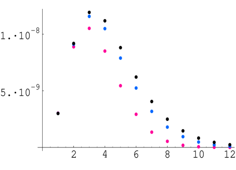
Figure 1: Spectrum $M^{5}\times\Gamma(\omega)$ of massless emission from the rotating ring as a function of $N_{0}=2M\omega$, for $N=M^{2}=20$ (lower points), $N=50$ and $N=100$ (higher points). Here $g_{s}^{2}=0.1$ and $\alpha^{\prime}=4$.

Since the dominant channel is the one where the final state is a rotating ring of lower mass, the decay can be pictured as a rotating circular string whose radius gradually decreases as it loses energy by radiation.

For large $N_{0}$, the spectrum exponentially goes to zero. It is of the form (see appendix C)

$$\Gamma(\omega)\cong N^{-{5\over 2}}\ e^{-2N_{0}(2\log 2-1)}=N^{-{5\over 2}}\ e^{-{\omega\over T_{0}}}\ ,\ \ \$$ (3.46)

$$T_{0}\equiv{a_{0}\over M}\ ,\ \ \ a_{0}^{-1}=4(2\log 2-1)\ .$$

The exponential form of the spectrum at large $\omega$, and the presence of a maximum at finite frequency allows one to approximate the spectrum curve by a thermal spectrum by introducing a “grey body factor” $\sigma_{\rm grey}(\omega)$ defined by

$$\Gamma(\omega)={\rm const.}\ M^{-5}\omega^{d-1}\sigma_{\rm grey}(\omega,T_{0})\ {1\over e^{\omega\over T_{0}}-1}\ ,$$

i.e.

$$\sigma_{\rm grey}(\omega,T_{0})\equiv M^{5}\Gamma(\omega)\omega^{1-d}(e^{\omega\over T_{0}}-1)\ .$$

where $\Gamma(\omega)$ is the expression obtained in subsection 3.1. The grey body factor here is introduced of course artificially, but given the decay properties of the rotating ring, as a smooth radiation process with frequencies peaked at $\omega\sim M^{-1}$, it is useful to picture it as a thermal radiation process, even if the exact spectrum formula is actually more complicated.

We have seen that the spectrum can be also obtained by a classical computation; the fact that it is peaked at small frequencies is in agreement with the classical analysis of [3] in the case of a smooth antenna.

We have also examined the spectrum of the string state with maximum angular momentum $(b^{\dagger}\tilde{b}^{\dagger})^{N}|0\rangle$. In this case we find that the spectrum does not resemble a thermal spectrum, in particular, it is not exponentially suppressed at large frequencies (more precisely, in the region $1\ll N_{0}\ll N$).

4 Presence of D branes

A question of interest is what is the lifetime of the rotating ring in the presence of D branes. Here we show that generically the ring cannot break into open string fragments, with Neumann or Dirichlet boundary conditions, nor in the presence of generic fluxes.

Moreover the rotating ring cannot either decay into another closed string plus open string fragments. All these processes are exponentially suppressed, i.e they are of order $O(e^{-M^{2}})$.

There is an exceptional case in which the breaking is not exponentially suppressed, namely if there is a D brane tilted with an angle equal to $\pm{\pi/4}$ with respect to the $Z_{1}$ and the $Z_{2}$ planes. This configuration is equivalent to a D brane such that its projection in the $Z_{1},Z_{2}$ subspace appears as a D4 brane with a suitable flux.

We begin by discussing the picture by the classical world-sheet equations. The classical solution corresponding to the circular string is given in eq. (3.4), which we repeat for convenience:

$$X^{c}_{j}=G_{j}(\tau-\sigma)\ ,\ \ \ \ X^{c}_{k}=G_{k}(\tau+\sigma)\ ,$$ (4.1)

where $j=1,2$ and $k=3,4$, with $G_{1,3}(x)=L\ \cos(x),\ G_{2,4}(x)=L\ \sin(x)$.

The classical equations are second order in $\tau$ therefore the breaking must require continuity in $\tau$ of the classical functions and of their first derivative (see [12]). In particular, this initial condition ensures that the Virasoro constraints are satisfied for the outgoing fragments. This initial condition holds for every coordinate.

Take generically an open string to be of the form $X^{open}(\tau,\sigma)=f(\tau+\sigma)+g(\tau-\sigma)$. For ${\cal N}$ Neumann or ${\cal D}$ Dirichlet boundary condition $g(x)=\pm f(x)$, but we consider more general cases resulting from rotations or presence of fluxes.

Suppose that at time $\tau=0$ the closed string breaks and it becomes an open string. The initial condition requires

$$Z^{c}(0,\sigma) = Z^{open}(0,\sigma)=f(\sigma)+g(-\sigma)\ ,$$ (4.2)

$$\partial_{\tau}Z^{c}(0,\sigma) = \mp\partial_{\sigma}Z^{c}(0,\sigma)=\partial_{\tau}Z^{open}(0,\sigma)=f^{\prime}(\sigma)+g^{\prime}(-\sigma)\ .$$ (4.3)

with $\mp=-$ for the $j$ and $=+$ for the $k$ components. Since the continuity requirement (4.2) must hold for every $\sigma$, we can take the derivative with respect to $\sigma$ and get

$$\partial_{\sigma}Z^{c}(0,\sigma)=f^{\prime}(\sigma)-g^{\prime}(-\sigma)\ .$$ (4.4)

Combining (4.3) with (4.4) one finds $\{f^{\prime}(x)\}_{m}=0$ for $m=j$ and $\{g^{\prime}(x)\}_{m}=0$ for $m=k$ . Therefore the only possible final open strings are those of the form $g(\tau-\sigma)$ in the $Z_{1}$ plane and $f(\tau+\sigma)$ in the $Z_{2}$ plane.

There is an exceptional case in which this is possible, namely when in the $Z_{1},Z_{2}$ subspace there is a D brane that in the $Z_{1},Z_{2}$ subspace it appears as a D2 brane at an angle of $\pm{\pi/4}$ with respect to the $Z_{1},Z_{2}$ planes. Using prime coordinates to denote the rotated system which is aligned with the D brane (located at, say, $Z_{2^{\prime}}=0$), one has

$$Z_{1^{\prime}}=\cos\theta\ g(\tau-\sigma)+\sin\theta\ f(\tau+\sigma)\ ,\ \ \ Z_{2^{\prime}}=-\sin\theta\ g(\tau-\sigma)+\cos\theta\ f(\tau+\sigma)\ .$$ (4.5)

The coordinate $Z_{1^{\prime}}$ satisfies the ${\cal N}$ boundary conditions provided $\cos\theta g(x)=\sin\theta f(x)$. The coordinate $Z_{2^{\prime}}$ satisfies the ${\cal D}$ boundary conditions provided $\cos\theta f(x)=\sin\theta g(x)=\sin\theta\tan\theta f(x)$, i.e. provided $\tan^{2}\theta=1$, implying $\theta=\pm{\pi/4}$. Note that in the rotated system the ring solution becomes

$$Z_{1^{\prime}}=\sqrt{2}L\ e^{i\tau}\cos\sigma\ ,\ \ \ \ Z_{2^{\prime}}=\sqrt{2}L\ e^{i\tau}\sin\sigma\ .$$ (4.6)

Thus, with this D brane configuration at a special angle, the circular string can break into an open string. Successively, the open string can easily break in more fragments. This configuration is equivalent to a D brane such that on the $Z_{1},Z_{2}$ subspace it appears as a D4 brane with a flux $F_{13}=F_{24}=1$.

Quantum mechanically, a classically forbidden process can occur via tunnelling, but it will be exponentially suppressed for large mass (i.e. large $L$). To see this, we use the boundary state formalism. Omitting world-sheet fermions and ghosts, a general D brane is represented by the boundary state

$$|B\rangle=e^{-\alpha^{{\dagger}}_{\cal N}\cdot\tilde{\alpha}^{{\dagger}}_{\cal N}+\alpha^{{\dagger}}_{\cal D}\cdot\tilde{\alpha}^{{\dagger}}_{\cal D}}|0\rangle\ ,$$ (4.7)

where $\alpha_{\cal N,D}$ indicate the space coordinate mode operators with ${\cal N}$ or ${\cal D}$ boundary conditions. We restrict our attention to the $Z_{1},Z_{2}$ subspace and consider a D-brane such that its projection on it is a D2 brane along the plane $X_{1^{\prime}}X_{2^{\prime}}$ :

$$|B\rangle=e^{-\alpha^{{\dagger}}_{1^{\prime}}\tilde{\alpha}^{{\dagger}}_{1^{\prime}}-\alpha^{{\dagger}}_{2^{\prime}}\tilde{\alpha}^{{\dagger}}_{2^{\prime}}+\alpha^{{\dagger}}_{3^{\prime}}\tilde{\alpha}^{{\dagger}}_{3^{\prime}}+\alpha^{{\dagger}}_{4^{\prime}}\tilde{\alpha}^{{\dagger}}_{4^{\prime}}}|0\rangle\ .$$ (4.8)

Here all $\alpha$ operators refer to the world-sheet mode operators of frequency 1; the coordinate indices $1^{\prime},2^{\prime},3^{\prime},4^{\prime}$ appear as subindices for clarity in the notation. Write

$$\alpha_{1^{\prime}} = \cos(\theta)\alpha_{1}+\sin(\theta)\alpha_{3}\ ,\ \ \ \ \alpha_{3^{\prime}}=-\sin(\theta)\alpha_{1}+\cos(\theta)\alpha_{3}\ ,$$ (4.9)

$$\alpha_{2^{\prime}} = \cos(\theta)\alpha_{2}-\sin(\theta)\alpha_{4}\ ,\ \ \ \ \alpha_{4^{\prime}}=\sin(\theta)\alpha_{2}+\cos(\theta)\alpha_{4}\ .$$

Then with our notation $b_{\pm}^{\dagger}={\alpha_{1}^{\dagger}\pm i\alpha_{2}^{\dagger}\over\sqrt{2}}$ , $c_{\pm}^{\dagger}={\alpha_{3}^{\dagger}\pm i\alpha_{4}^{\dagger}\over\sqrt{2}}$ we get,

$$|B\rangle=e^{-\sin(2\theta)(b_{+}^{{\dagger}}\tilde{c}_{+}^{{\dagger}}+c_{+}^{{\dagger}}\tilde{b}_{+}^{{\dagger}}+b_{-}^{{\dagger}}\tilde{c}_{-}^{{\dagger}}+c_{-}^{{\dagger}}\tilde{b}_{-}^{{\dagger}})+\cos(2\theta)(-b_{+}^{{\dagger}}\tilde{b}_{-}^{{\dagger}}-b_{-}^{{\dagger}}\tilde{b}_{+}^{{\dagger}}+c_{+}^{{\dagger}}\tilde{c}_{-}^{{\dagger}}+c_{-}^{{\dagger}}\tilde{c}_{+}^{{\dagger}})}|0\rangle\ .$$ (4.10)

Therefore, the amplitude for the process in which the ring is “absorbed” by the brane thus becoming open strings on it, is

$$A=\langle 0|{(b_{+}\tilde{c}_{+})^{N}\over N!}|B\rangle=(-\sin(2\theta))^{N}\ .$$ (4.11)

Thus this process is exponentially suppressed unless $\theta=\pm\pi/4$.

The rotating ring could still decay into open strings in a two-step process in which the ring first decays into a left-right symmetric (or antisymmetric) closed string state by emitting a closed string mode. Then the resulting (anti) symmetric closed string state can decay into two open strings.

To calculate this process, we need to specify the emitted closed string state. Emission of massive particles from the ring are exponentially suppressed. One could still wonder if the process could take place by emission of a massless particle. We now show that this process is even more suppressed, like $N^{-2N}$.

We first consider an example, where we assume that the left-right symmetric closed string state is

$$|\Phi^{\prime}_{N^{\prime}}\rangle\equiv{1\over(N^{\prime}/2)!^{2}}(b^{\dagger}c^{\dagger})^{{N^{\prime}\over 2}}(\tilde{b}^{\dagger}\tilde{c}^{\dagger})^{{N^{\prime}\over 2}}|0\rangle\ .$$

Then we need to evaluate the matrix element

$$A_{R}={1\over(N^{\prime}/2)!\sqrt{N!}}\langle 0|(bc)^{{N^{\prime}\over 2}}:\xi.\partial X(1)e^{ik.X(1)}:{b^{\dagger}}^{N}|0\rangle\ .$$ (4.12)

The calculation is straightforward and the final result is

$$A_{R}=-i\sqrt{2}\varepsilon\sqrt{N!}(-\sqrt{2}\kappa)^{N-{N^{\prime}\over 2}-1}(\sqrt{2}\bar{\tilde{\kappa}})^{N^{\prime}\over 2}\sum_{r=0}^{N^{\prime}/2}{(-2\kappa\bar{\kappa})^{r}\over r!(N-{N^{\prime}\over 2}+r-1)!({N^{\prime}\over 2}-r)!}+\cdots$$ (4.13)

where dots stand for a similar term which is of the same order. To see the large $N$ behavior, one can consider the two cases, $N-N^{\prime}=N_{0}$=fixed, or $N^{\prime}$=fixed. Using the Stirling approximation, in both cases we find $A_{R}=O(N^{-N})$. One reason why this is so small is the factorial in the denominator $(N-{N^{\prime}\over 2}+r-1)!$ that starts from $({N\over 2}+{N_{0}\over 2}-1)!$, which is large. The only way that this would not be large is if the final state is similar to the ring state insofar as it contains $b^{N_{1}}$ and $\tilde{c}^{N_{2}}$ with both $N-N_{1}$ and $N-N_{2}$ small. But such states are far from being left-right symmetric or antisymmetric. They are small deformations of the rotating ring.

One could consider more general emitted closed string states of the form $(b^{\dagger}\tilde{b}^{\dagger})^{N_{1}}(c^{\dagger}\tilde{c}^{\dagger})^{N_{2}}|0\rangle$, $N_{1}+N_{2}=N^{\prime}$. Since in this case we cannot have both $N-N_{1}$ and $N-N_{2}$ small, we again expect a similar suppression. In particular, consider the extreme case $(b^{\dagger}\tilde{b}^{\dagger})^{N^{\prime}}$, i.e. $N_{2}=0$. This represents a decay of the rotating ring into the closed string state of maximum angular momentum, which, being a folded left-right symmetric string may successively decay into open strings by breaking. By a similar computation we find that the matrix element is of order $O(N^{-2N})$ for $N-N^{\prime}=N_{0}$=fixed and of order $O(N^{-N})$ for $N^{\prime}$=fixed. As expected for the reasons explained above, the process is suppressed.

Thus we conclude that, except for a brane configuration at a special angle, the decay rate of the rotating ring in presence of D branes is still dominated by a decay into a similar ring state of lower mass by massless emission. The lifetime of the ring is therefore given by the formula of section 3.1, ${\cal T}_{\rm ring}=c_{0}g_{s}^{-2}\ M^{5}$.

5 Case of compactified dimensions

The results can be easily extended to the case in which some $d_{c}$ dimensions have been compactified. When some dimensions are compactified, type II superstring theories can have many exactly stable perturbative and non-perturbative states, associated with supersymmetric branes or supersymmetric fundamental strings wrapping cycles (in ten uncompact dimensions, only the D0 branes of type IIA have finite mass). Here we are interested in the stability of non-supersymmetric configurations. We will focus on the rotating ring, since this seems to be the most stable non-supersymmetric (zero charge) state. We have explicitely considered the torus compactification, but the pattern is generic. We assume that the radii $R_{i}$ of the compact dimensions are much smaller than the length $L=\sqrt{\alpha^{\prime}N\over 2}$ of our circular string (its mass is $M={2\sqrt{N}\over\sqrt{\alpha^{\prime}}}$, $N$ being a large integer). In the opposite case, the circular string does not feel the effect of the compactification and we have the same results as in the uncompactified case.

When two or more dimensions are compact, we have two different scenarios according to whether the compact dimensions occur in both the $Z_{1}$ and $Z_{2}$ planes, where the circular string lies, or not. In fact, in the former case, say that $X_{1}$ in the $Z_{1}$ plane and $X_{3}$ in the $Z_{2}$ plane are compact, the circular string will wind around $X_{1}$ with its Right part and around $X_{3}$ with its Left part, and it will easily break into winding modes.

Instead, if the compact dimensions occur only in one of the above planes, say in $Z_{1}$, then it is impossible for the circular string to break into winding modes in the $Z_{1}$ plane while respecting the Virasoro constraints, since classically the Left part in the $Z_{2}$ plane would remain unbroken. Quantum mechanically, this process is expected to be suppressed exponentially for large length of the circular string.

This has been numerically verified by extending the computation of [5] to the case of two compact dimensions [13].

Therefore, if the compact dimensions occur only in one of the planes, say $Z_{1}$, the dominant decay channel will be by emission of radiation.

It is easy to extend our operatorial computation of Section 3 to the case in which some $d_{c}$ dimensions are compactified. If no compact dimension occurs in the $Z_{1,2}$ planes, then the only modifications are the integration over the angles, because now we have to integrate $\int d\Omega_{8-d_{c}}$ in the place of $\int d\Omega_{8}$, and in the phase-space factor, which is now $\omega^{7-d_{c}}M^{-2}\prod_{i}^{d_{c}}R_{i}^{-1}$ in the place of $\omega^{7}M^{-2}$, because the momentum of the emitted massless particle becomes $9-d_{c}$ dimensional. In fact we can neglect the possibility of emitting a particle with Kaluza-Klein momentum as it would be effectively massive and thus exponentially suppressed.

The result is that the radiation spectrum is still described by a scaling expression

$$\Gamma\sim g_{s}^{2}{\alpha^{\prime}}^{4}M^{2}\ \omega^{7-d_{c}}\left(\prod_{i}^{d_{c}}R_{i}^{-1}\right)\ f_{d_{c}}(\alpha^{\prime}M\omega)\ .$$ (5.1)

The form of $f_{d_{c}}(x)$ depends on $d_{c}$, the number of compactified dimensions. The total radiation rate is obtained by summing over the integer $N_{0}={\alpha^{\prime}\over 2}M\omega$ getting

$$\Gamma_{\rm tot}\sim g_{s}^{2}{\alpha^{\prime}}^{(d_{c}-6)/2}M^{-(5-d_{c})}\prod_{i}^{d_{c}}{\sqrt{\alpha^{\prime}}\over R_{i}}\ .$$ (5.2)

If some of the $d_{c}$ dimensions occur say in the $Z_{1}$ plane, the pattern is the same as before, but the scaling function $f_{d_{c}}(x)$ is further modified by the fact that some among the momentum components $k_{1}$ and $k_{2}$, which appear in the expression giving $f_{d_{c}}(x)$, are set to zero. If both the dimensions of the $Z_{1}$ plane are compact and thus $k_{1}=k_{2}=0$, we see from the expression of the Right contribution to the spectrum (3.10), (3.11) that only $N_{0}=1$ survives, that is, the spectrum is in this case a single point:

$$\omega={2\over\alpha^{\prime}M}\ .$$ (5.3)

and the final state is similar to the initial one with the change $M^{2}={4\over\alpha^{\prime}}N\to M_{1}^{2}={4\over\alpha^{\prime}}(N-1)$.

Consider, in particular, $d_{c}=6$ (corresponding to $3+1$ uncompact dimensions). In the case the circular string lies on the uncompact dimensions in its, say, Right part and on a compact plane in its Left part, and its length is much larger than every compactification radius, it decays by emitting a massless particle of energy (5.3) and changing its length from $\sqrt{\alpha^{\prime}N\over 2}$ to $\sqrt{\alpha^{\prime}(N-1)\over 2}$. This emission process takes a time ${\cal T}\sim{1\over g_{s}^{2}M}\prod_{i}^{6}{R_{i}\over\sqrt{\alpha^{\prime}}}$.

The total time it takes to reduce its size from $N$ large to $N^{\prime}$ of the order of some units, and thus easily breaking and disappearing, is obtained by integrating ${dN\over dt}\sim 1/{\cal T}$ from $N$ to $0$. We obtain

$${\cal T}_{\rm tot}\sim N\ {\cal T}\cong{\alpha^{\prime}M\over g_{s}^{2}}\prod_{i}^{6}{R_{i}\over\sqrt{\alpha^{\prime}}}\ .$$ (5.4)

In a generic case in which some $6-d_{sc}$ radii are much larger than the circular string length $L$ and $d_{sc}$ radii are of order $O(\alpha^{\prime})$, the total time it takes for the string to decay completely in massless modes is

$${\cal T}_{\rm tot}\sim{N\over\langle N_{0}\rangle}\ {\cal T}\cong{1\over g_{s}^{2}}{\alpha^{\prime}}^{(4-{d_{sc}\over 2})}M^{(7-d_{sc})}\prod_{i}^{d_{sc}}{R_{i}\over\sqrt{\alpha^{\prime}}}\ .$$ (5.5)

since now $N$ will decrease on average by a finite amount $\langle N_{0}\rangle$ of the order of unity in a single radiation step.

6 Lifetime of average string state

The lifetime of the average string state can be obtained by computing the decay rate averaged over all initial states of the same mass $M$. Here we will compute the average decay rate for massless emission, and neglect the decay channel into two massive particles. Thus this will give an upper bound for the lifetime of the average string state.

The average decay rate for massless emission was computed in [9] for the bosonic string. Here we generalize this calculation to the type II superstring.

We are going to compute an amplitude of the form

$$\bar{\Gamma}={\rm const.}\ g_{s}^{2}{\omega^{7}\over M^{2}}\ \sigma_{R}\ \sigma_{L}\ ,\ \ \ \ \omega={M^{2}-{M^{\prime}}^{2}\over 2M}={N_{0}\over 2\sqrt{N}}\ ,$$ (6.1)

where

$$\sigma_{R}={1\over\mathcal{N}_{N_{R}}}\oint_{C}{dz^{\prime}\over z^{\prime}}z^{\prime-N^{\prime}}\oint_{C^{\prime}}{dz\over z}z^{-N}{\rm Tr}[{{\hbox{1\kern-2.27621ptl}}+e^{i\pi F}\over 2}V_{R}^{\dagger}(k,1){{\hbox{1\kern-2.27621ptl}}+e^{i\pi F}\over 2}z^{\prime\hat{N}}V_{R}(k,1)z^{\hat{N}}]\ .$$ (6.2)

$V_{R}$ is the vertex operator (2.7) and $\mathcal{N}_{N_{R}}$ is the number of states at level $N=N_{R}=N_{L}$ in the NS-NS sector. Asymptotically,

$$\mathcal{N}_{N_{R}}={\rm const.}\ N_{R}^{-{(D+1)\over 4}}e^{a\sqrt{N_{R}}}\ ,\ \ \ \ a=\pi\sqrt{D-2}\ ,$$

with $D=10$ space-time dimensions. We introduce a basis of coherent states:

$$|\{\lambda_{n}\}\rangle=\prod_{n=1}^{\infty}\exp[\lambda_{n}\cdot\alpha_{n}^{\dagger}]|0;p\rangle\ ,\ \ \ \ |\{\theta_{r}\}\rangle=\prod_{r=1-\nu}^{\infty}\exp[\theta_{r}\cdot\psi_{r}^{\dagger}]|0;p\rangle\ ,$$ (6.3)

where $\theta_{r}$ are Grassmann variables. Defining

$$\Sigma_{\bar{\lambda},\lambda,\bar{\theta},\theta} \equiv {1\over\mathcal{N}_{N}}\oint_{C}{dz^{\prime}\over z^{\prime}}z^{\prime-N^{\prime}}\oint_{C^{\prime}}{dz\over z}z^{-N}$$

$$\times \langle\{\lambda_{n}\},\{\theta_{r}\}|{{\hbox{1\kern-2.27621ptl}}+e^{i\pi F}\over 2}V_{R}^{\dagger}(k,1){{\hbox{1\kern-2.27621ptl}}+e^{i\pi F}\over 2}z^{\prime\hat{N}}V_{R}(k,1)z^{\hat{N}}|\{\lambda_{n}\},\{\theta_{r}\}\rangle\ ,$$

then the trace can be computed by integrating over all $\bar{\lambda}_{n},\lambda_{n}$ and $\bar{\theta}_{r},\ \theta_{r}$ with the weight factor $e^{-\bar{\theta}_{r}\cdot\theta_{r}}e^{-\bar{\lambda}_{n}\cdot\lambda_{n}}$ due to normalization.

A shortcut to the calculation is to note that the following terms in (6.2) do not contribute to the trace:

$$\sum_{\Phi_{N}}\langle\Phi_{N}|\xi.\psi k.\psi{z^{\prime}}^{\hat{N}}\xi.\psi\ k.\psi|\Phi_{N}\rangle=0\ ,\ \ \ \ \sum_{\Phi_{N}}\langle\Phi_{N}|\xi.\psi\ k.\psi|\Phi_{N}\rangle=0\ .$$ (6.5)

The reason why these terms vanish is that they must be proportional to $\xi.k$ or $k^{2}$ by Lorentz invariance. It is interesting to note that these correlators are not zero for particular states such as the rotating ring, but the whole expression vanishes after taking the trace. As a result, only the $\partial X$ part of the vertex contributes. Then, since there is no fermion insertion, the fermion part in (6.2) gives the standard fermion partition function. What remains is the bosonic part computed in [9] plus the ghost contributions, which are implicit in (6.2).

In this case it is important to consider explicitely the ghosts, ensuring that we only keep physical states. In the $bc$ ghost sector, we compute the amplitude (Right part)

$$\sigma_{R}=\sum_{\Omega_{N},\Omega_{N^{\prime}}}\langle\Omega_{N}|c(1)|\Omega_{N^{\prime}}\rangle\langle\Omega_{N^{\prime}}|c(1)|\Omega_{N}\rangle\ ,$$ (6.6)

where $c(1)$ is the ghost field associated with the vertex operator $V(k,1)$ in (2.7) and $|\Omega_{N^{\prime}}\rangle$ are “physical” ghost states (that is, such that the matter times ghost states satisfy the physical conditions). We then write:

$$\sum_{\Omega_{N^{\prime}}}|\Omega_{N^{\prime}}\rangle\langle\Omega_{N^{\prime}}|=\oint{dz\over z}z^{\hat{N}-{N^{\prime}}}b_{0}(\sum_{\Psi}|\Psi\rangle\langle\Psi|)=\oint{dz\over z}z^{\hat{N}-{N^{\prime}}}b_{0}{\hbox{1\kern-2.27621ptl}}\ \ ,$$ (6.7)

where the $|\Psi\rangle$ are all states built with $b,c$ oscillators. The projector on states of level $N^{\prime}$ is the same of (2.3) (here we use its ghost part), the $b_{0}$ insertion is due to the fact that while the sum $\sum_{\Psi}$ is over all of the ghost states, the physical ones must satisfy the condition $b_{0}|\Omega\rangle=0$. These states, thanks to the $b,c$ algebra, can be written as $b_{0}|\Psi\rangle$ where $|\Psi\rangle$ is any ghost state. Thus we have to compute

$$A={\rm Tr}[(-1)^{F_{g}}c(1)b_{0}c(z)z^{\prime\hat{N}}z^{\hat{N}}]\ ,$$ (6.8)

where $F_{g}$ anticommutes with all ghost modes.

This can be done with the same coherent state formalism described above. The final result is

$$A=\prod_{n=1}^{\infty}(1-w^{n})^{2},\quad w=z^{\prime}z\ .$$ (6.9)

The superghost part of the average state computation gives directly the superghost partition function (since the vertex operators $V(k,1),V(k,z)$ do not carry any superghost contribution).

The result is thus

$$\sigma_{R}={\xi\cdot\xi(N-N^{\prime})\over\mathcal{N}_{N}}\oint{dz\over z}{z^{-{N^{\prime}}}f(z)^{2-D}\over 1-z^{N-N^{\prime}}}\left({1\over\sqrt{z}}g_{3}(z)^{D-2}-{1\over\sqrt{z}}g_{4}(z)^{D-2}+g_{2}(z)^{D-2}\right)\ ,$$ (6.10)

where

$$f(z)=\prod_{n=1}^{\infty}(1-z^{n})\,\ \ \ g_{3}(z)=\prod_{r={1\over 2}}^{\infty}(1+z^{r})\ ,\ \ \ g_{4}(z)=\prod_{r={1\over 2}}^{\infty}(1-z^{r})\,\ \ \ g_{2}(z)=\prod_{r=0}^{\infty}(1+z^{r})\ .$$ (6.11)

For large $N^{\prime}$ the integral (6.10) can be computed by a saddle point approximation, the main contribution coming from $z\sim 1$. The computation is similar to the calculation of the asymptotic level density $\mathcal{N}_{N}$ for level $N$. The behavior of the different functions in (6.11) at $z\sim 1$ follows from the modular properties of the theta functions. We find

$$f(z)\cong{\rm const.}(1-z)^{-{1\over 2}}e^{-{\pi^{2}\over 6(1-z)}}\ ,\ \ \ \ g_{3}(z)\cong{\rm const.}\ e^{{\pi^{2}\over 12(1-z)}}\ ,$$ (6.12)

$$g_{4}(z)\cong{\rm const.}\ e^{-{\pi^{2}\over 3(1-z)}}\ ,\ \ \ \ g_{2}(z)\cong{\rm const.}\ e^{{\pi^{2}\over 12(1-z)}}\ .$$ (6.13)

The saddle point is at $\ln z\cong-{a\over 2\sqrt{N^{\prime}}}$ with $a=\pi\sqrt{D-2}$. Using $N-N^{\prime}=2\omega\sqrt{N}$, $\alpha^{\prime}=4$, we obtain for large $N^{\prime}$:

$$\sigma_{R}(\omega)\cong\xi\cdot\xi\ \omega M\ {e^{a\sqrt{N-2\omega\sqrt{N}}-a\sqrt{N}}\over 1-e^{-a\omega}}\cong\xi\cdot\xi\ \omega M\ {e^{-a\omega}\over 1-e^{-a\omega}}\ .$$ (6.14)

Thus, by eq. (6.1), the average decay amplitude is given by

$$\bar{\Gamma}={\rm const.}\ g_{s}^{2}\xi^{2}\tilde{\xi}^{2}\ \sigma_{\rm grey}(\omega,T)\ {1\over e^{\omega\over T}-1}\ \omega^{8}\ ,$$ (6.15)

where $T={1\over a\sqrt{\alpha^{\prime}}}$ is the Hagedorn temperature of type II superstring theory and $\sigma_{\rm grey}(\omega)$ is a grey body factor given by

$$\sigma_{\rm grey}(\omega,T)=\omega{1-e^{-{\omega\over T}}\over(1-e^{-{\omega\over 2T}})(1-e^{-{\omega\over 2T}})}\ .$$ (6.16)

Thus an average superstring state in type II superstring theory emits radiation as a grey body at the Hagedorn temperature. In the case of type I open superstrings, the spectrum for massless vector emission is obtained from the right part (6.14), i.e.

$$\bar{\Gamma}_{\rm I}(\omega)\cong\xi\cdot\xi\ M^{-1}\ {e^{-{\omega\over T_{\rm I}}}\over 1-e^{-{\omega\over T_{\rm I}}}}\ \omega^{8}\ ,$$ (6.17)

where $T_{\rm I}={2\over a\sqrt{\alpha^{\prime}}}$ is the Hagedorn temperature of type I superstring theory. Hence average states in type I superstrings emit radiation as a perfect black body.

To compute the total average decay rate, one sums over all $N_{0}$. Recalling that $\omega=N_{0}/2M$, this sum can be approximated by an integral over $\omega$ by introducing the differential $2Md\omega$. We find

$$\bar{\Gamma}_{\rm tot}\sim g_{s}^{2}\ M\ .$$ (6.18)

Since $\bar{\Gamma}$ represents the average decay rate taking into account massless emission only, the lifetime of an average state has the upper bound

$$\bar{\cal T}\leq g_{s}^{-2}\ M^{-1}\ .$$ (6.19)

The same result holds for the bosonic and heterotic string theory.

7 Discussion

The average lifetime computed here, $\bar{\cal T}\leq M^{-1}$, shows that most of the massive states at each mass level have a short lifetime, which decreases for larger masses. There can only be a few states at each mass level whose lifetime increases with the mass. Some of these few states are given by the family of states $|\Phi_{n,k}\rangle$, $N=2k$, studied in [5], interpolating between the rotating ring $n=k$ and the state $n=0$. The corresponding classical configurations describe rotating elliptical strings, which become circular for $n=k$ and a folded, straight closed string for $n=0$. For generic $n$ one finds that the lifetime ${\cal T}$ also increases with the mass, though at much lower rate for states that significantly differ from the rotating ring (i.e. states with $n$ not close to $k$). When $n\ll k$, the ellipse is very eccentrical and the decay by breaking into two massive string states becomes the dominant channel. These are all states of high angular momentum.

The law ${\cal T}_{\rm ring}\cong{\rm const.}\ M^{5}$ has been derived in four independent ways. 1) By evaluation of the imaginary part of the two-point function [5], 2) by operator calculation of the full massless emission rate, 3) by operator calculation of the dominant decay channel into a ring of lower mass and 4) by classical radiation from the rotating string soliton configuration. The latter also confirms the identification of the quantum state with the string soliton.

The rotating ring has the special feature that it decays predominantly into another rotating ring, i.e. the decay can be viewed as a rotating circular string whose radius gradually decreases as it emits radiation. The decay rate of the rotating ring has the scaling property $\Gamma=cg_{s}^{2}\ M^{-(5-d_{c})}\ \bar{f}(N_{0})$, where $N_{0}=M^{2}-{M^{\prime}}^{2}=2\omega M$, $d_{c}=$ number of compact dimensions with radius $R<<\alpha^{\prime}M$, and a spectrum sharing some qualitative features with a thermal spectrum, such as an exponential tail. This is not the case e.g. for the state of maximum angular momentum $(b^{\dagger}\tilde{b}^{\dagger})^{N}|0\rangle$.

In the case of the average state, one finds as in [9] that the spectrum becomes exactly thermal in the large mass limit and that the average type II superstring emits radiation as a grey body with temperature equal to the Hagedorn temperature (while the average type I superstring behaves as a perfect black body at the Hagedorn temperature).

Appendix A Notation

We consider type II superstring theory in the NS formulation. The world-sheet action is given by

$$S={1\over 2\pi\alpha^{\prime}}\int d^{2}z\big{(}\partial X^{\mu}\bar{\partial}X_{\mu}+\psi^{\mu}\bar{\partial}\psi_{\mu}+\tilde{\psi}^{\mu}\partial\tilde{\psi}_{\mu}\big{)}$$ (A.1)

We will be interested in string states corresponding to excitations in two planes,

$$Z^{1}=\frac{X^{1}+iX^{2}}{\sqrt{2}},\ \ Z^{2}=\frac{X^{3}+iX^{4}}{\sqrt{2}}\ ,$$

$$\psi^{Z_{1}}=\frac{\psi^{1}+i\psi^{2}}{\sqrt{2}},\ \ \psi^{Z_{2}}=\frac{\psi^{3}+i\psi^{4}}{\sqrt{2}}\ .$$

The expansion for the bosonic world sheet fields are as follows

$$Z_{R}^{1}={i}\sqrt{\frac{\alpha^{\prime}}{2}}\sum_{n=1}^{\infty}{1\over\sqrt{n}}\big{[}b_{n-}z^{-n}-b_{n+}^{\dagger}z^{n}\big{]}\ ,\ \ \ Z_{L}^{1}={i}\sqrt{\frac{\alpha^{\prime}}{2}}\sum_{n=1}^{\infty}{1\over\sqrt{n}}\big{[}\tilde{b}_{n-}\bar{z}^{-n}-\tilde{b}_{n+}^{\dagger}\bar{z}^{n}\big{]}\ ,$$

$$Z_{R}^{2}={i}\sqrt{\frac{\alpha^{\prime}}{2}}\sum_{n=1}^{\infty}{1\over\sqrt{n}}\big{[}c_{n-}z^{-n}-c_{n+}^{\dagger}z^{n}\big{]}\ ,\ \ \ Z_{L}^{2}={i}\sqrt{\frac{\alpha^{\prime}}{2}}\sum_{n=1}^{\infty}{1\over\sqrt{n}}\big{[}\tilde{c}_{n-}\bar{z}^{-n}-\tilde{c}_{n+}^{\dagger}\bar{z}^{n}\big{]}\ ,$$

$$[b_{n\pm},b_{m\pm}^{\dagger}]=\delta_{nm}\ ,\ \ [\tilde{b}_{n\pm},\tilde{b}_{m\pm}^{\dagger}]=\delta_{nm}\ ,\ \ [c_{n\pm},c_{m\pm}^{\dagger}]=\delta_{nm}\ ,\ \ [\tilde{c}_{n\pm},\tilde{c}_{m\pm}^{\dagger}]=\delta_{nm}\ .$$

For the fermion fields, we have

$$\psi^{Z_{i}}=\sqrt{\alpha^{\prime}\over 2}\sum_{r}\psi_{r}^{Z_{i}}z^{-r}\ ,\ \ \ \tilde{\psi}^{Z_{i}}=\sqrt{\alpha^{\prime}\over 2}\sum_{r}\tilde{\psi}_{r}^{Z_{i}}\bar{z}^{-r}\ ,$$ (A.2)

$$\{\psi_{r}^{Z_{i}},\psi_{s}^{Z_{j}}\}=\delta_{rs}\delta_{ij}\ .$$

The mass formula is given by

$$\alpha^{\prime}M^{2}=2(\hat{N}_{R}+\hat{N}_{L})\ ,\ \ \ \ \ N_{R}=N_{L}\ ,$$ (A.3)

where the number operators are

$$\hat{N}_{R}=\sum_{n=1}^{\infty}n(b_{n+}^{\dagger}b_{n+}+b_{n-}^{\dagger}b_{n-}+c_{n+}^{\dagger}c_{n+}+c_{n-}^{\dagger}c_{n-})+\sum_{r={1\over 2}}^{\infty}r\psi_{-r}^{Z_{i}}\psi_{r}^{Z_{i}}-a_{0}\ .$$ (A.4)

The expression for $\hat{N}_{L}$ is similar, with the obvious changes. The normal ordering constant $a_{0}$ is $a_{0}=1/2$ in the NS sector and $a_{0}=0$ in the R sector.

The basic correlators are

$$\langle\partial_{w}X(w)\partial_{z}X(z)\rangle=-{\alpha^{\prime}\over 2}{zw\over(w-z)^{2}}\ ,\ \ \ \ \ \langle\psi(w)\psi(z)\rangle={\alpha^{\prime}\over 2}{(zw)^{1/2}\over w-z}\ .$$ (A.5)

We use the following angular coordinates

$$\hat{x}_{1}=\sin\theta\cos\alpha\cos\beta\cos\varphi\ ,\ \ \ \ \hat{x}_{2}=\sin\theta\cos\alpha\cos\beta\sin\varphi\ ,$$

$$\hat{x}_{3}=\sin\theta\cos\alpha\sin\beta\cos\psi\ ,\ \ \ \ \hat{x}_{4}=\sin\theta\cos\alpha\sin\beta\sin\psi\ ,$$

$$\hat{x}_{5}=\sin\theta\sin\alpha\cos\beta^{\prime}\cos\varphi^{\prime}\ ,\ \ \ \ \hat{x}_{6}=\sin\theta\sin\alpha\cos\beta^{\prime}\sin\varphi^{\prime}\ ,$$

$$\hat{x}_{7}=\sin\theta\sin\alpha\sin\beta^{\prime}\cos\psi^{\prime}\ ,\ \ \hat{x}_{8}=\sin\theta\sin\alpha\sin\beta^{\prime}\sin\psi^{\prime}\ ,\ \ \hat{x}_{9}=\cos\theta\ .$$

Thus the volume element is

$$d^{8}\Omega=\sin^{7}\theta\cos^{3}\alpha\sin^{3}\alpha\cos\beta\sin\beta\cos\beta^{\prime}\sin\beta^{\prime}d\theta d\alpha d\beta d\varphi d\psi d\beta^{\prime}d\varphi^{\prime}d\psi^{\prime}$$

In order to sum over polarizations, we use the relations

$$\sum_{\xi}\xi^{i}\xi^{j}=\delta^{ij}-{k^{i}k^{j}\over|\vec{k}|^{2}}\ ,\ \ \ \ \sum_{\xi}\xi^{i}\xi_{i}=d-1=8\ .$$ (A.6)

This gives ($\kappa$ and $\varepsilon$ are defined in (3.5), (3.6) )

$$\sum_{\xi}\varepsilon^{2}=-{\kappa^{2}\over|\vec{k}|^{2}}\ ,\ \ \ \ \sum_{\xi}\bar{\varepsilon}^{2}=-{\bar{\kappa}^{2}\over|\vec{k}|^{2}}\ ,\ \ \ \sum_{\xi}\varepsilon\bar{\varepsilon}=1-{\kappa\bar{\kappa}\over|\vec{k}|^{2}}\ .$$ (A.7)

Writing

$$2\kappa^{2}={N_{0}^{2}\over 4N}\ e^{2i\varphi}v^{2}\ ,\ \ \ v^{2}\equiv\sin^{2}\theta\cos^{2}\alpha\cos^{2}\beta\ ,$$

we have

$$\sum_{\xi}\varepsilon^{2}=-e^{2i\varphi}{v^{2}\over 2}\ ,\ \ \ \ \sum_{\xi}\bar{\varepsilon}^{2}=-\ e^{-2i\varphi}{v^{2}\over 2},\ \ \ \sum_{\xi}\varepsilon\bar{\varepsilon}=1-{v^{2}\over 2}\ .$$ (A.8)

Appendix B Other contributions to the decay rate of the rotating ring

The remaining contributions to the decay rate of the rotating ring indicated in section 3.1 are

$$\sigma_{2} = -i{1\over N!}\oint{dz\over z}\ z^{N_{0}}\langle 0|b^{N}e^{-ik.X(1)}e^{ik.X(z)}\xi.\partial X(1){b^{\dagger}}^{N}|0\rangle\langle 0|\psi_{1\over 2}^{\bar{Z}}\xi.\psi(z)k.\psi(z)\psi_{-{1\over 2}}^{Z}|0\rangle\ ,$$

$$\sigma_{3} = i{1\over N!}\oint{dz\over z}\ z^{N_{0}}\langle 0|b^{N}e^{-ik.X(1)}e^{ik.X(z)}\xi.\partial X(z){b^{\dagger}}^{N}|0\rangle\langle 0|\psi_{1\over 2}^{\bar{Z}}\xi.\psi(1)k.\psi(1)\psi_{-{1\over 2}}^{Z}|0\rangle\ ,$$

$$\sigma_{4} = -{1\over N!}\oint{dz\over z}\ z^{N_{0}}\langle 0|b^{N}e^{-ik.X(1)}e^{ik.X(z)}{b^{\dagger}}^{N}|0\rangle\langle 0|\psi_{1\over 2}^{\bar{Z}}\xi.\psi(1)k.\psi(1)\ \xi.\psi(z)k.\psi(z)\psi_{-{1\over 2}}^{Z}|0\rangle\ ,$$

$$\sigma_{5} = {1\over N!}\oint{dz\over z}\ z^{N_{0}}\langle 0|b^{N}e^{-ik.X(1)}e^{ik.X(z)}{b^{\dagger}}^{N}|0\rangle\langle 0|\xi.\partial X(1)\xi.\partial X(z)|0\rangle\langle 0|\psi_{1\over 2}^{\bar{Z}}\psi_{-{1\over 2}}^{Z}|0\rangle$$

Computing the matrix elements, we find

$$\sigma_{2}=-4\oint{dz\over z}z^{N_{0}}\big{(}(\bar{\varepsilon}\varepsilon\bar{\kappa}\kappa-\bar{\varepsilon}^{2}\kappa^{2})z^{-1}+(\varepsilon^{2}\bar{\kappa}^{2}-\bar{\varepsilon}\varepsilon\bar{\kappa}\kappa)\big{)}\sum_{m=0}^{N-1}{N!(2\kappa\bar{\kappa})^{m}\over m!(m+1)!(N-m-1)!}{(1-z)^{2m+1}\over z^{m}}\ ,$$

$$\sigma_{4}=4\xi\cdot\xi\ \kappa\bar{\kappa}\oint{dz\over z}z^{N_{0}}\sum_{m=0}^{N}{N!(2\kappa\bar{\kappa})^{m}\over m!^{2}(N-m)!}\big{[}{(1-z)^{2m-1}\over z^{m}}-{(1-z)^{2m-1}\over z^{m-1}}\big{]}\ ,$$

$$\sigma_{5}=2\xi\cdot\xi\oint{dz}z^{N_{0}}\sum_{m=0}^{N}{N!(2\kappa\bar{\kappa})^{m}\over m!^{2}(N-m)!}{(1-z)^{2m-2}\over z^{m}}\ ,$$

and $\sigma_{3}=\sigma_{2}^{*}$. Expanding the binomials $(1-z)$ and computing the integral over $z$, we find

$$\sigma_{2}=4\!\!\sum_{m=N_{0}-1}^{N-1}\!{(-1)^{m-N_{0}}N!(2m+1)!(2\kappa\bar{\kappa})^{m}\big{[}(\bar{\varepsilon}\varepsilon\bar{\kappa}\kappa\!\!-\!\!\varepsilon^{2}\bar{\kappa}^{2})(m-\!\!N_{0}+\!\!1)\!\!-\!\!(\bar{\varepsilon}^{2}\kappa^{2}\!\!-\!\!\bar{\varepsilon}\varepsilon\bar{\kappa}\kappa)(m+N_{0}+1)\big{]}\over m!(m+1)!(N-m-1)!(m-N_{0}+1)!(m+N_{0}+1)!}\ ,$$

$$\sigma_{4}=4\xi\cdot\xi\ \kappa\bar{\kappa}\sum_{m=N_{0}}^{N}{(-1)^{m-N_{0}}N!(2m)!(2\kappa\bar{\kappa})^{m}\over m!^{2}(N-m)!(m-N_{0})!(m+N_{0})!}\ ,$$

$$\sigma_{5}=-2\xi\cdot\xi\sum_{m=N_{0}+1}^{N}{(-1)^{m-N_{0}}N!(2m-2)!\ (2\kappa\bar{\kappa})^{m}\over m!^{2}(N-m)!(m+N_{0}-1)!(m-N_{0}-1)!}\ .$$

Now we can estimate which is the dominant contribution in the large $N$ limit, with fixed $N-N^{\prime}$. Using Stirling formula (3.24) and the fact that $\kappa\kappa\sim N^{-1}$, we see that the dominant term is $\sigma_{1}$, with $\sigma_{1}=O(N)$. Similary, we see that $\sigma_{2},\sigma_{3},\sigma_{5}$ are of order $O(1)$ and $\sigma_{4}$ is of order $O(N^{-1})$ (the explicit numerical evaluation shows that $\sigma_{2},...,\sigma_{5}$ are two or more orders of magnitudes smaller than $\sigma_{1}$ already for $N=20$). The application of the Stirling formula is justified in the present case because decays with $N_{0}\gg 1$ are always suppressed as long as $N$ is large.

Appendix C Tail of the spectrum

We consider the expression for $\Sigma_{11}$ (3.18). Using the Stirling formula (3.24), we find

$$\Sigma_{11}=\sqrt{\pi}N^{2}x^{2N_{0}}\sum_{r,s=0}^{\infty}{(-x)^{r+s}\over\Gamma(2N_{0}+r+s+{13\over 2})}a(r)a(s)\ ,$$ (C.1)

$$a(r)={(2r+2N_{0})!\over r!(N_{0}-1+r)!(r+2N_{0})!}\ ,$$

where $x\equiv 2\kappa\bar{\kappa}N={N_{0}^{2}\over 4}$. We are interested in the large $N_{0}$ behavior of this sum. Because the series converges very rapidly, we can approximate

$${(2N_{0}+2r)!\over(2N_{0}+r)!}\cong(2N_{0})^{r}\ ,\ \ \ {(2N_{0}+2s)!\over(2N_{0}+s)!}\cong(2N_{0})^{s}\ .$$ (C.2)

At the same time, we use Stirling formula to approximate

$$\Gamma(2N_{0}+r+s+{13\over 2}) \cong (2N_{0})!\ (2N_{0})^{r+s+{11\over 2}}$$ (C.3)

$$\cong \sqrt{2\pi}(2N_{0})^{2N_{0}+r+s+6}\ e^{-2N_{0}}\ .$$

We find

$$\Sigma_{11}\cong N^{2}{x^{2N_{0}}\over\sqrt{2}}{e^{2N_{0}}\over(2N_{0})^{2N_{0}+6}}\ S(N_{0})^{2}\ ,$$ (C.4)

$$S(N_{0})\equiv\sum_{r=0}^{\infty}{(-x)^{r}\over r!(N_{0}-1+r)!}\ .$$ (C.5)

We can write this sum as

$$S(N_{0})={1\over 2\pi i}\oint{dt\over t}\ t^{N_{0}-1}\ \exp[-xt+{1\over t}]\ ,\ \ \ \ x={N_{0}^{2}\over 4}\ .$$ (C.6)

The integral can be computed by saddle-point approximation, with the result

$$S(N_{0})={\rm const.}\ N_{0}^{\beta}\ e^{N_{0}\log 2-N_{0}\log N_{0}}\ ,$$ (C.7)

where $\beta$ is a constant of order one. Adding the phase space factor, we finally obtain

$$\Gamma_{11}={1\over M^{2}}\omega^{7}\Sigma_{11}=N\big{(}{N_{0}\over 2\sqrt{N}}\big{)}^{7}N_{0}^{2\beta-6}e^{-2N_{0}(2\log 2-1)}\ ,$$ (C.8)

i.e.

$$\Gamma_{11}=N^{-{5\over 2}}\ N_{0}^{1+2\beta}\ e^{-2N_{0}(2\log 2-1)}\ .$$ (C.9)

Similarly, one can consider $\Sigma_{22}$ and $\Sigma_{12}$. We find the same behavior.

References

• [1] E. Witten, “Cosmic Superstrings,” Phys. Lett. B 153, 243 (1985).
• [2] E. J. Copeland, R. C. Myers and J. Polchinski, JHEP 0406, 013 (2004) [arXiv:hep-th/0312067].
• [3] T. Damour and A. Vilenkin, Phys. Rev. D 64, 064008 (2001) [arXiv:gr-qc/0104026].
• [4] T. W. B. Kibble, “Cosmic strings reborn?,” arXiv:astro-ph/0410073.
• [5] D. Chialva, R. Iengo and J. G. Russo, “Decay of long-lived massive closed superstring states: Exact results,” JHEP 0312, 014 (2003) [arXiv:hep-th/0310283].
• [6] J. Dai and J. Polchinski, Phys. Lett. B 220, 387 (1989).
• [7] D. Mitchell, N. Turok, R. Wilkinson and P. Jetzer, Nucl. Phys. B 315, 1 (1989) [Erratum-ibid. B 322, 628 (1989)].
• [8] H. Okada and A. Tsuchiya, Phys. Lett. B 232, 91 (1989).
• [9] D. Amati and J. G. Russo, “Fundamental strings as black bodies,” Phys. Lett. B 454, 207 (1999) [arXiv:hep-th/9901092].
• [10] J. L. Manes, “Emission spectrum of fundamental strings: An algebraic approach,” Nucl. Phys. B 621, 37 (2002) [arXiv:hep-th/0109196].
• [11] J. L. Manes, “String form factors,” JHEP 0401, 033 (2004) [arXiv:hep-th/0312035].
• [12] R. Iengo and J. G. Russo, “Semiclassical decay of strings with maximum angular momentum,” JHEP 0303, 030 (2003) [arXiv:hep-th/0301109].
• [13] D. Chialva and R. Iengo, “Long lived large type II strings: Decay within compactification,” JHEP 0407, 054 (2004) [arXiv:hep-th/0406271].
• [14] S. Weinberg, “Gravitation and Cosmology”, (Wiley, New York, 1972).