Walls and vortices in supersymmetric
non-abelian gauge theories

Abstract

We review recent results (hep-th/0405194, hep-th/0405129, and hep-th/0404198) on the BPS multi-wall solutions in supersymmetric $U(N_{\rm C})$ gauge theories in five dimensions with $N_{\rm F}(>N_{\rm C})$ hypermultiplets in the fundamental representation. Total moduli space of the BPS non-Abelian walls is found to be the complex Grassmann manifold $SU(N_{\rm F})/[SU(N_{\rm C})\times SU(N_{\rm F}-{N}_{\rm C})\times U(1)]$. Exact solutions are obtained with full generic moduli for infinite gauge coupling. A $1/4$ BPS equation is also solved, giving vortices together with the non-Abelian walls and monopoles in the Higgs phase attached to the vortices. The full moduli space of the $1/4$ BPS solutions is found to be holomorphic maps from a complex plane to the wall moduli space.

1 Introduction

Supersymmetry (SUSY) is useful to obtain various branes (solitons) for model building in the brane-world scenario[1, 2, 3]. The partial preservation of SUSY gives BPS states which are solutions of equations of motion[4]. Moreover, the resulting theory tends to produce an $N=1$ SUSY theory on the world volume, which can provide realistic unified models with the desirable properties[5]. SUSY also helps to obtain stability of the soliton. The simplest soliton for the brane-world is the domain wall, which should be considered in five dimensions. Recently the localized massless gauge bosons on a wall has been obtained using SUSY QED interacting with hypermultiplets and tensor multiplets[6, 7]. We anticipate that walls in non-Abelian gauge theories will help to obtain localized non-Abelian gauge bosons. These walls are called non-Abelian walls, and are interesting in its own right.

We review our papers on various BPS solutions of the SUSY $U(N_{\rm C})$ gauge theory with $N_{\rm F}(>N_{\rm C})$ flavors of hypermultiplets in the fundamental representation in spacetime dimensions of five or less[8, 9, 10, 11]. To obtain discrete vacua, we consider non-degenerate masses $m_{A}$ for hypermultiplets $H^{irA}$, and the Fayet-Iliopoulos (FI) parameter is introduced[12]. We have obtained BPS multi-wall solutions as $1/2$ BPS solutions, and various combinations of walls, vortices and monopoles in the Higgs phase as $1/4$ BPS solutions. By taking the limit of infinite gauge coupling, we have obtained exact BPS multi-wall solutions with generic moduli parameters covering the complete moduli space of walls[8]. We found that the moduli space of $1/2$ BPS domain walls is given by a compact complex manifold, the Grassmann manifold[8] $G_{N_{\rm F},N_{\rm C}}\equiv{SU(N_{\rm F})\over SU(N_{\rm C})\times SU(N_{\rm F}-N_{\rm C})\times U(1)}$. One should note that this is the total moduli space of the multi-wall solutions including all the topological sectors, and that configurations with smaller number of domain walls appear as boundaries of the moduli space. We have found that the coexistence of mutually orthogonal vortex and the wall can be realized as a $1/4$ BPS configuration[9]. We also found that this $1/4$ BPS equation admits monopoles in the Higgs phase which were found recently[13]. We have obtained the exact solitons in the limit of infinite gauge coupling. We also identified the moduli space to be all the holomorphic maps from the complex plane to the wall moduli space[9], the Grassmann manifold $G_{N_{\rm F},N_{\rm C}}$.

2 Vacua and BPS Equations for Non-Abelian Walls

Discrete vacua are needed for walls and can be realized by mass terms for hypermultiplets and $U(N_{\rm C})$ gauge group with the $U(1)$ factor group allowing the Fayet-Iliopoulos term[12]. We consider a five-dimensional SUSY model with minimal kinetic terms for vector and hypermultiplets whose physical bosonic fields are ($W_{M},\Sigma$) and $H^{i}$, respectively. We denote space-time indices by $M,N,\cdots=0,1,2,3,4$ with the metric $\eta_{MN}={\rm diag}(+1,-1,-1,-1,-1)$. For simplicity, we take the same gauge coupling $g$ for $U(1)$ and $SU(N_{\rm C})$ factors. The $N_{\rm F}$ flavors of hypermultiplets in the fundamental representation are combined into an $N_{\rm C}\times N_{\rm F}$ matrix. We consider $N_{\rm F}>N_{\rm C}$ to obtain disconnected SUSY vacua[12] appropriate for constructing walls. Our model now has only a few parameters: the gauge coupling constant $g$, the FI parameter $c>0$ for the $U(1)$ gauge group, and the mass matrix of hypermultiplets $(M)^{A}{}_{B}\equiv m_{A}\delta^{A}{}_{B}$ $m_{A}$. We assume non-degenerate mass parameters with the ordering $m_{A}>m_{A+1}$ for all $A$. Then the flavor symmetry reduces to $G_{\rm F}=U(1)_{\rm F}^{N_{\rm F}-1}$. After eliminating auxiliary fields, we obtain the bosonic part of the Lagrangian and the scalar potential

$${L}_{\rm bosonic} = -\frac{1}{2g^{2}}{\rm Tr}\left[F_{MN}F^{MN}\right]+\frac{1}{g^{2}}{\rm Tr}\left[{D}_{M}\Sigma{D}^{M}\Sigma\right]$$ (1)

$$+{\rm Tr}\left[{D}^{M}H^{i}({D}_{M}H^{i})^{\dagger}\right]-V,$$

$$V = \frac{g^{2}}{4}{\rm Tr}\Big{[}\left(H^{1}H^{1\dagger}-H^{2}H^{2\dagger}-c\mathbf{1}_{N_{\rm C}}\right)^{2}+4H^{2}H^{1\dagger}H^{1}H^{2\dagger}\Big{]}$$ (2)

$$+{\rm Tr}\left[(\Sigma H^{i}-H^{i}M)(\Sigma H^{i}-H^{i}M)^{\dagger}\right],$$

The covariant derivatives are defined as $D_{M}\Sigma=\partial_{M}\Sigma+i[W_{M},\Sigma]$, $D_{M}H^{i}=(\partial_{M}+iW_{M})H^{i}$, and field strength is defined as $F_{MN}=\frac{1}{i}[D_{M},D_{N}]=\partial_{M}W_{N}-\partial_{N}W_{M}+i[W_{M},W_{N}]$.

SUSY vacua are realized at vanishing vacuum energy, which requires both contributions from vector and hypermultiplets to vanish. Conditions of vanishing contribution from vector multiplet read

$$H^{1}H^{1\dagger}-H^{2}H^{2\dagger}=c\mathbf{1}_{N_{\rm C}},\quad H^{2}H^{1\dagger}={0}.$$ (3)

The vanishing contribution to vacuum energy from hypermultiplets gives the SUSY condition for hypermultiplets as

$$\Sigma H^{i}-H^{i}M=0,\$$ (4)

for each index $A$. Non-degenerate masses for hypermultiplets dictate that only one flavor $A=A_{r}$ can be non-vanishing for each color component $r$ of hypermultiplet scalars $H^{irA}$ with

$$H^{1rA}=\sqrt{c}\,\delta^{A_{r}}{}_{A},\quad H^{2rA}=0.$$ (5)

This is called the color-flavor locking vacuum. The vector multiplet scalars $\Sigma$ are determined as

$$\Sigma={\rm diag.}(m_{A_{1}},\,m_{A_{2}},\,\cdots,\,m_{A_{N_{\rm C}}}).$$ (6)

We denote a SUSY vacuum specified by a set of non-vanishing hypermultiplet scalars with the flavor $\{A_{r}\}$ for each color component $r$ as $\langle A_{1}\,A_{2}\,\cdots\,A_{N_{\rm C}}\rangle$. We usually take $A_{1}<A_{2}<\cdots<A_{N_{\rm C}}$.

Walls interpolate between two vacua at $y=\infty$ and $y=-\infty$. These boundary conditions at $y=\pm\infty$ define topological sectors. To obtain domain walls, we assume that all fields depend only on coordinate of one extra dimension $x^{4}\equiv y$ and the Poincaré invariance on the four-dimensional world volume of the wall. It implies $F_{MN}(W)=0$, $W_{\mu}=0$, where $x^{\mu}=(x^{0},x^{1},x^{2},x^{3})$ are four-dimensional world-volume coordinates. Note that $W_{y}$ need not vanish. The Bogomol’nyi completion of the energy density of our system can be performed as

$${E} = {1\over g^{2}}{\rm Tr}\left({D}_{y}\Sigma-{g^{2}\over 2}\left(c{\bf 1}_{N_{\rm C}}-H^{1}H^{1}{}^{\dagger}+H^{2}H^{2}{}^{\dagger}\right)\right)^{2}+{g^{2}}{\rm Tr}\Big{[}H^{2}H^{1\dagger}H^{1}H^{2\dagger}\Big{]}$$ (7)

$${}+{\rm Tr}\left[({D}_{y}H^{1}+\Sigma H^{1}-H^{1}M)({D}_{y}H^{1}+\Sigma H^{1}-H^{1}M)^{\dagger}\right]$$

$${}+{\rm Tr}\left[({D}_{y}H^{2}-\Sigma H^{2}+H^{2}M)({D}_{y}H^{2}-\Sigma H^{2}+H^{2}M)^{\dagger}\right]$$

$${}+c\partial_{y}{\rm Tr}\Sigma-\partial_{y}\left\{{\rm Tr}\left[\left(\Sigma H^{1}-H^{1}M\right)H^{1}{}^{\dagger}+\left(-\Sigma H^{2}+H^{2}M\right)H^{2}{}^{\dagger}\right]\right\}.$$

Therefore we obtain a lower bound for the energy of the configuration by saturating the complete squares. The saturation condition gives the BPS equations

$$D_{y}\Sigma={g^{2}\over 2}\left(c{\bf 1}_{N_{\rm C}}-H^{1}H^{1}{}^{\dagger}+H^{2}H^{2}{}^{\dagger}\right),\quad 0=g^{2}H^{1}H^{2}{}^{\dagger},$$ (8)

$$D_{y}H^{1}=-\Sigma H^{1}+H^{1}M,\qquad D_{y}H^{2}=\Sigma H^{2}-H^{2}M.$$ (9)

Let us consider a configuration approaching to a SUSY vacuum labeled by $\langle A_{1}A_{2}\cdots A_{N_{\rm C}}\rangle$ at the boundary of positive infinity $y=+\infty$, and to a vacuum $\langle B_{1}B_{2}\cdots B_{N_{\rm C}}\rangle$ at the boundary of negative infinity $y=-\infty$. Therefore the minimum energy is achieved by the configuration satisfying the BPS Eqs. (8)-(9), and the energy for the BPS saturated configuration is given by

$$T_{\rm w} = \int^{+\infty}_{-\infty}dy\;{E}=c\left[{\rm Tr}\Sigma\right]^{+\infty}_{-\infty}=c\left(\sum_{k=1}^{N_{\rm C}}m_{A_{k}}-\sum_{k=1}^{N_{\rm C}}m_{B_{k}}\right),$$ (10)

the second term of the last line of Eq. (7) does not contribute, since the vacuum condition $\Sigma H^{i}-H^{i}M=0$ is satisfied at $y=\pm\infty$. The BPS equations are equivalent to the preservation of $1/2$ SUSY[8].

3 BPS Multi-Walls

With our sign choice of the FI parameter $c>0$, $H^{2}$ vanishes in any SUSY vacuum. The BPS equation for $H^{2}$ gives[10] $H^{2}=0$, and $H^{2}_{0}=0$. By defining a complex $N_{\rm C}\times N_{\rm C}$ invertible matrix function $S(y)$

$$\Sigma+iW_{y}\equiv S^{-1}\partial_{y}S,$$ (11)

we can solve the hypermultiplet BPS equation in terms of a $N_{\rm C}\times N_{\rm F}$ constant complex matrix $H_{0}$ as integration constants, which we call moduli matrices:

$$H^{1}=S^{-1}H_{0}^{1}e^{My}.$$ (12)

Two different sets ($S,H_{0}$) and $(S^{\prime},H_{0}{}^{\prime})$ give the same original fields $\Sigma,\,W_{y},H^{i}$, if they are related by $V\in GL(N_{\rm C},{\bf C})$

$$S \rightarrow S^{\prime}=VS,\quad H_{0}^{1}\rightarrow H_{0}^{1}{}^{\prime}=VH_{0}^{1}.$$ (13)

This transformation $V$ defines an equivalence class among sets of the matrix function and moduli matrix $(S,H_{0})$ which represent physically equivalent results. This symmetry comes from the $N_{\rm C}^{2}$ integration constants in solving (11), and represents the redundancy of describing the wall solution in terms of $(S,H_{0})$. We call this ‘world-volume symmetry’,

The gauge transformations on the original fields $\Sigma,\,W_{y},\,H^{1},$ ($H^{1}\rightarrow H^{1}{}^{\prime}=UH^{1}$, $\Sigma+iW_{y}\rightarrow\Sigma^{\prime}+iW_{y}^{\prime}=U\left(\Sigma+iW_{y}\right)U^{\dagger}+U\partial_{y}U^{\dagger}$) can be obtained by multiplying a unitary matrix $U^{\dagger}$ $S\,\rightarrow\,S^{\prime}=SU^{\dagger}$, $U^{\dagger}U=1$, without causing any transformations on the moduli matrices $H_{0}$. Thus we define $\Omega\equiv SS^{\dagger}$, which is invariant under the gauge transformations $U$ of the fundamental theory. Together with the gauge invariant moduli matrix $H_{0}$, the BPS equations (8) for vector multiplets can be rewritten in the following gauge invariant form

$$\partial_{y}^{2}\Omega-\partial_{y}\Omega\Omega^{-1}\partial_{y}\Omega=g^{2}\left(c\,\Omega-H_{0}\,e^{2My}H_{0}{}^{\dagger}\right).$$ (14)

We can calculate uniquely the $N_{\rm C}\times N_{\rm C}$ complex matrix $S$ from the $N_{\rm C}\times N_{\rm C}$ Hermitian matrix $\Omega$ with a suitable gauge choice. Then all the quantities, $\Sigma,\,W_{y},\,H^{1}$ and $H^{2}$ are obtained by Eqs. (11) and (12).

Since we are going to impose two boundary conditions at $y=\infty$ and at $y=-\infty$ to the second order differential equation (14), the number of necessary boundary conditions precisely matches to obtain the unique solution. Therefore there should be no more moduli parameters in addition to the moduli matrix $H_{0}$. In the limit of infinite gauge coupling, we find explicitly that there are no additional moduli. We have also analyzed in detail the almost analogous nonlinear differential equation in the case of the Abelian gauge theory at finite gauge coupling and find no additional moduli[6]. Thus we believe that we should consider only the moduli contained in the moduli matrix $H_{0}$, in order to discuss the moduli space of domain walls.

4 Moduli Space and Exact Solution for Non-Abelian Walls

All possible solutions of parallel domain walls in the $U(N_{\rm C})$ SUSY gauge theory with $N_{\rm F}$ hypermultiplets can be constructed once the moduli matrix $H_{0}$ is given. The moduli matrix $H_{0}$ has a redundancy expressed as the world-volume symmetry (13) : $H_{0}\sim VH_{0}$ with $V\in GL(N_{\rm C},{\bf C})$. We thus find that the moduli space denoted by ${M}_{N_{\rm F},N_{\rm C}}$ is homeomorphic to the complex Grassmann manifold ($\tilde{N}_{\rm C}\equiv N_{\rm F}-N_{\rm C}$):

$${M}_{N_{\rm F},N_{\rm C}} \simeq \{H_{0}|H_{0}\sim VH_{0},V\in GL(N_{\rm C},{\bf C})\}$$ (15)

$$\simeq G_{N_{\rm F},N_{\rm C}}\simeq{SU(N_{\rm F})\over SU(N_{\rm C})\times SU(\tilde{N}_{\rm C})\times U(1)}\,.$$

This is a compact (closed) set. On the other hand, scattering of two Abelian walls is described by a nonlinear sigma model on a non-compact moduli space[14, 15, 6]. This fact can be consistently understood, if we note that the moduli space ${M}_{N_{\rm F},N_{\rm C}}$ includes all BPS topological sectors:

$${M}_{N_{\rm F},N_{\rm C}}=\sum_{k=0}^{N_{\rm C}\tilde{N}_{\rm C}}{M}_{N_{\rm F},N_{\rm C}}^{k}={M}_{N_{\rm F},N_{\rm C}}^{0}\oplus{M}_{N_{\rm F},N_{\rm C}}^{1}\oplus\cdots\oplus{M}_{N_{\rm F},N_{\rm C}}^{N_{\rm C}\tilde{N}_{\rm C}},$$ (16)

where ${M}_{N_{\rm F},N_{\rm C}}^{k}$ is the moduli space of $k$-walls. Consider a $k$-wall solution and imagine a situation such that one of the outer-most walls goes to spatial infinity. We will obtain a ($k-1$)-wall configuration in this limit. This implies that the $k$-wall sector in the moduli space is an open set compactified by the moduli space of ($k-1$)-wall sectors on its boundary. Continuing this procedure we will obtain a single wall configuration. Pulling it out to infinity we obtain a vacuum state in the end. A vacuum corresponds to a point as a boundary of a single wall sector in the moduli space. Summing up all sectors, we thus obtain the total moduli space ${M}_{N_{\rm F},N_{\rm C}}$ as a compact manifold.

The BPS equation (14) for the gauge invariant $\Omega$ reduces to an algebraic equation in the strong gauge coupling limit, given by

$$\Omega_{g\to\infty}=(SS^{\dagger})_{g\to\infty}=c^{-1}H_{0}e^{2My}H_{0}^{\dagger}.$$ (17)

Qualitative behavior of walls for finite gauge couplings is not so different from that in infinite gauge couplings. In fact we have constructed exact wall solutions for finite gauge couplings[6] and found that their qualitative behavior is the same as the infinite gauge coupling cases found in the literature[14, 16].

SUSY gauge theories reduce to nonlinear sigma models in general in the strong gauge coupling limit $g\to\infty$. This is the HK nonlinear sigma model on the cotangent bundle over the complex Grassmann manifold[17, 12]

$${M}^{M=0}_{\rm vac}\simeq T^{*}G_{N_{\rm F},N_{\rm C}}\simeq T^{*}\left[SU(N_{\rm F})\over SU(N_{\rm C})\times SU(\tilde{N}_{\rm C})\times U(1)\right]\,.$$ (18)

From the target manifold (18) one can easily see that there exists a duality between theories with the same flavor and two different gauge groups in the case of the infinite gauge coupling[18, 12]: $U(N_{\rm C})\leftrightarrow U(\tilde{N}_{\rm C})$ with $\tilde{N}=N_{\rm F}-N_{\rm C}$. This duality holds for the Lagrangian of the nonlinear sigma models, and leads to the duality of the BPS equations for these two theories. This duality holds also for the moduli space of domain wall configurations.

We can obtain the effective action on the world volume of walls, by promoting the moduli parameters to fields on the world volume [19]. In the case of infinite gauge coupling, the Kähler potential of the effective Lagrangian is given by [10]

$${L}_{\rm walls}=c\int d^{4}\theta\int dy\log\det\Omega=c\int d^{4}\theta\int dy\log\det(H_{0}e^{2My}H_{0}{}^{\dagger}).$$ (19)

5 Meaning of the Moduli Matrix $H_{0}$ and Vortices

To illustrate the physical meaning of the moduli matrix, we first consider the Abelian gauge group $N_{\rm C}=1$. The moduli matrix in this case can be parametrized as

$$H_{0}=\sqrt{c}(e^{r_{1}},e^{r_{2}},\cdots,e^{r_{N_{F}}}),$$ (20)

where $e^{r_{A}}$ are complex moduli parameters. Let us note that the first entry can be fixed to $e^{r_{1}}=1$ by using the world-volume symmetry (13). Then we obtain the hypermultiplet scalars as

$$H=S^{-1}H_{0}e^{My}=S^{-1}\sqrt{c}(e^{r_{1}+m_{1}y},\cdots,e^{r_{N_{F}}+m_{N_{F}}y}).$$ (21)

The $y$ dependence due to the masses of the hypermultiplet flavors shows that the relative magnitude of different flavors varies as $y$ varies, indicating that the solution approaches various vacua at various $y$. The transition between two adjacent vacua occurs when two different flavors becomes comparable to each other. This transition region is precisely where the wall separating two vacua is located. The wall location separating $A$- and $A+1$-th vacua is then determined in terms of the relative magnitude of different flavors of the moduli matrix elements as ${\rm Re}r_{A}+m_{A}y\sim{\rm Re}r_{A+1}+m_{A+1}y$. The overall normalization is taken care of by the function $S^{-1}(y)$. Consequently the hypermultiplet scalars exhibit the multi-wall behavior as illustrated in Fig. 1 for the case of $N_{\rm F}=4$.

Figure 1: Region of rapid change of hypermultiplets indicates the positions of walls.

Similar consideration applies to non-Abelian case. The only difference is that some of the matrix elements of the moduli matrix $H_{0}$ can be made to vanish by means of the world-volume symmetry (13). The topological sector with the maximal number of moduli is given by the vanishing left-lower and right-upper triangular parts[10]. Therefore the dimension of the moduli space is given by

$$\dim_{\bf C}{M}_{N_{\rm F},N_{\rm C}}\equiv N_{\rm C}N_{\rm F}-N_{\rm C}^{2}=N_{\rm C}\tilde{N}_{\rm C}.$$ (22)

We have also found interesting characteristic behavior of the non-Abelian walls. Depending on the quantum numbers of the wall, two walls can pass through each other, maintaining their identity. We call these pair as penetrable walls[10]. On the other hand, certain combinations of walls cannot penetrate each other, resulting in impenetrable walls. If two walls are impenetrable, two walls are compressed each other when the relative distance moduli becomes negative infinity. In the case of Abelian gauge theories, only the impenetrable walls can occur[6, 14, 15].

If we make the moduli matrix $H_{0}$ in Eq.(20) to depend on the world volume coordinates, the wall location should depend on the position on the world volume. Then the walls will be curved in general. If we have a zero in $H_{0}$, it will give us a spike-like behavior of the wall, which becomes a vortex ending at the wall[20]. As expected for vortices, magnetic fields are also generated at the same time. Similarly, if we allow an exponential dependence on the world volume coordinates for the moduli matrix elements, the wall can tilt and a magnetic field is generated along the tilted wall. In fact we have found that the addition of vortex perpendicular to the walls can preserve $1/2$ of the surviving SUSY on the world volume of the wall. Consequently the combined configuration preserves $1/4$ of the original SUSY. We also found that the $1/4$ BPS equation allows another BPS object, the monopole in the Higgs phase, which was found recently[13].

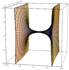
Figure 2: Surfaces defined by the same energy density : a) A vortex stretched between walls with $H_{0}(z)e^{Mx^{3}}=\sqrt{c}(e^{x^{3}},ze^{4},e^{-x^{3}})$. b) A vortex attached to a tilted wall with $H_{0}(z)e^{Mx^{3}}=\sqrt{c}(z^{2}e^{x^{3}},e^{-1/2z})$. Note that there are two surfaces with the same energy for each wall.

We find that the moduli space of solutions of this $1/4$ BPS equations is all the holomorphic maps from a complex plane to the wall moduli space, the deformed complex Grassmann manifold $G_{N_{\rm F},N_{\rm C}}={SU(N_{\rm F})\over SU(N_{\rm C})\times SU(\tilde{N}_{\rm C})\times U(1)}$ in Eq.(15). We can obtain exact solutions in the limit of infinite gauge coupling[9]. As an illustrative example, we show a vortex connecting two walls, and a vortex ending on a tilted wall in Fig.2. In the example Fig.2a), the left-most vacuum outside of the wall and the right-most vacuum outside of the wall are different. They have to touch at the middle of the vortex. Therefore there must be a kink separating these two vacua. This is precisely analogous to the kink in the middle of the vortex, where a monopole in the Higgs phase resides[13]. The example in Fig.2b) gives a model for a noncommutative plane, since there is a magnetic flux flowing along the wall.

The authors thank Koji Hashimoto and David Tong for a useful discussion.

References

- [1] P. Horava and E. Witten, Nucl. Phys. B460, 506 (1996) [hep-th/9510209].
- [2] N. Arkani-Hamed, S. Dimopoulos and G. Dvali, Phys. Lett. B429, 263 (1998) [hep-ph/9803315]; I. Antoniadis, N. Arkani-Hamed, S. Dimopoulos and G. Dvali, Phys. Lett. B436, 257 (1998) [hep-ph/9804398].
- [3] L. Randall and R. Sundrum, Phys. Rev. Lett. 83, 3370 (1999) [hep-ph/9905221]; Phys. Rev. Lett. 83, 4690 (1999) [hep-th/9906064].
- [4] E. Witten and D. Olive, Phys. Lett. B78, 97 (1978).
- [5] S. Dimopoulos and H. Georgi, Nucl. Phys. B193, 150 (1981); N. Sakai, Z. f. Phys. C11, 153 (1981); E. Witten, Nucl. Phys. B188, 513 (1981); S. Dimopoulos, S. Raby and F. Wilczek, Phys. Rev. D24, 1681 (1981).
- [6] Y. Isozumi, K. Ohashi, and N. Sakai, JHEP 11, 060 (2003) [hep-th/0310189].
- [7] Y. Isozumi, K. Ohashi, and N. Sakai, JHEP 11, 061 (2003) [hep-th/0310130].
- [8] Y. Isozumi, M. Nitta, K. Ohashi, and N. Sakai, Phys. Rev. Lett. to appear [hep-th/0404198].
- [9] Y. Isozumi, M. Nitta, K. Ohashi, and N. Sakai, hep-th/0405129.
- [10] Y. Isozumi, M. Nitta, K. Ohashi, and N. Sakai, Phys. Rev. D to appear [hep-th/0405194].
- [11] Y. Isozumi, M. Nitta, K. Ohashi and N. Sakai, to appear in the Proceedings of SUSY2004 [hep-th/0409110].
- [12] M. Arai, M. Nitta and N. Sakai, hep-th/0307274; to appear in the Proceedings of the 3rd International Symposium on Quantum Theory and Symmetries (QTS3), September 10-14, 2003 [hep-th/0401084]; to appear in the Proceedings of the International Conference on “Symmetry Methods in Physics (SYM-PHYS10)” held at Yerevan, Armenia, 13-19 Aug. 2003 [hep-th/0401102]; to appear in the Proceedings of SUSY 2003 held at the University of Arizona, Tucson, AZ, June 5-10, 2003 [hep-th/0402065].
- [13] D. Tong, Phys. Rev. D69, 065003 (2004) [hep-th/0307302]; R. Auzzi, S. Bolognesi, J. Evslin, K. Konishi and A. Yung, Nucl. Phys. B673, 187 (2003) [hep-th/0307287]; R. Auzzi, S. Bolognesi, J. Evslin and K. Konishi, [hep-th/0312233]; M. Shifman and A. Yung, Phys. Rev. D70, 045004 (2004) [hep-th/0403149]; A. Hanany and D. Tong, JHEP 0404, 066 (2004) [hep-th/0403158].
- [14] D. Tong, Phys. Rev. D66, 025013 (2002) [hep-th/0202012].
- [15] D. Tong, JHEP 0304, 031 (2003) [hep-th/0303151].
- [16] E. Abraham and P. K. Townsend, Phys. Lett. B 291, 85 (1992); J. P. Gauntlett, D. Tong and P. K. Townsend, Phys. Rev. D64, 025010 (2001) [hep-th/0012178]; M. Arai, M. Naganuma, M. Nitta, and N. Sakai, Nucl. Phys. B652, 35 (2003) [hep-th/0211103]; in Garden of Quanta - In honor of Hiroshi Ezawa, Eds. by J. Arafune et al. (World Scientific Publishing Co. Pte. Ltd. Singapore, 2003) pp 299-325 [hep-th/0302028].
- [17] U. Lindström and M. Roček, Nucl. Phys. B222, 285 (1983).
- [18] I. Antoniadis and B. Pioline, Int. J. Mod. Phys. A12, 4907 (1997) [hep-th/9607058].
- [19] N. S. Manton, Phys. Lett. B110, 54 (1982).
- [20] J. P. Gauntlett, R. Portugues, D. Tong, and P.K. Townsend, Phys. Rev. D63, 085002 (2001) [hep-th/0008221].