Knotted Configurations with Arbitrary Hopf Index from the Eikonal Equation

Abstract

The complex eikonal equation in $(3+1)$ dimensions is investigated. It is shown that this equation generates many multi-knot configurations with an arbitrary value of the Hopf index. In general, these eikonal knots do not have the toroidal symmetry. For example, a solution with topology of the trefoil knot is found. Moreover, we show that the eikonal knots provide an analytical framework in which qualitative (shape, topology) as well as quantitative (energy) features of the Faddeev-Niemi hopfions can be captured. It might suggest that the eikonal knots can be helpful in construction of approximated (but analytical) knotted solutions of the Faddeev-Skyrme-Niemi model.

1 Introduction

Topological solitons i.e. stable, particle-like objects with a non-vanishing topological charge occur in various contexts of the theoretical physics. For example, as magnetic monopoles and vortices seem to play crucial role in the problem of the confinement of the quarks in the quantum chromodynamics [1], [2]. On the other hand, it is believed that other type of solitons so-called cosmic strings and domain walls are important for the time evolution of the universe and formation of long range structures [3], [4]. Moreover, as D-branes, they appear in the string theory as well. They are observed also in various experiments in the condensed matter physics (see for instance ${}^{3}He$ [5] and ${}^{4}He$ [6] quantum liquids). In fact, richness of the possible application of solitons is enormous.
In particular, hopfions i.e. topological solitons with the non-trivial Hopf index $Q_{H}\in\pi_{3}(S^{2})$ have been recently analyzed in a connection with the non-perturbative regime of the gluodynamics. Namely, it has been suggested by Faddeev and Niemi [8] that particles built only of the gauge field, so-called glueballs, can be described as knotted solitons with a non-vanishing value of the Hopf number. It is a natural extension of the standard flux-tube picture of mesons where, due to the dual Meissner effect, quark and anti-quark are confined by a tube of the gauge field. In the case of absence of quark sources, such a flux-tube should form a knotted, closed loop. Then, stability of the configuration would be guaranteed by a non-zero value of the topological charge. A model (so called the Faddeev-Skyrme-Niemi model [7]), based on an effective classical three component unit field (which is believed to represent all infrared important degrees of freedom of the full quantum theory) has been proposed [8], [9], [10], [11]. In fact, using some numerical methods many topological solitons with the Hopf index have been found [12], [13], [14]. However, since all Faddeev-Niemi knots are known only in the numerical form some crucial questions (e.g. their stability) are still far from a satisfactory understanding. The situation is even worse. For a particular value of the Hopf index it is not proved which knot gives the stable configuration. Because of the lack of the analytical solutions of the Faddeev-Skyrme-Niemi model such problems as interaction of hopfions, their scattering or formation of bound states have not been solved yet (for some numerical results see [15]).
On the other hand, in order to deal with hopfions in an analytical way, many toy models have been constructed [16], [17], [18], [19]. In general, all of them are invariant under the scaling transformation. It not only provides the existence of hopfions but also gives an interesting way to circumvent the Derrick theorem [20]. This idea is quite old and has been originally proposed by Deser et al. [21]. As a result, topological hopfions with arbitrary Hopf number have been obtained. Unfortunately, on the contrary to the Faddeev-Niemi knots, all toy hopfions possess toroidal symmetry i.e. surfaces of the constant $n^{3}$ are toruses (they are called ’unknots’). It strongly restricts applicability of these models.
The main aim of the present paper is to find a systematic way of construction of analytical configurations with the Hopf charge, which in general do not have the toroidal symmetry and can form really knotted structures, as for instance the trefoil knot observed in the Faddeev-Skyrme-Niemi effective model. Moreover, our approach allows us to construct multi-knot configurations, where knotted solutions are linked and form even more complicated objects.
Moreover, though obtained here knots do not satisfy the Faddeev-Skyrme-Niemi equations of motion, there are arguments which allow us to believe that our solutions (we call them as eikonal knots) can have something to do with Faddeev-Niemi hopfions. In our opinion this paper can be regarded as a first step in construction of analytical topological solutions in the Faddeev-Skyrme-Niemi model. The relation between the eikonal knots and the Faddeev-Niemi hopfions will be discussed more detailed in the last section.
Our paper is organized as follows. In section 2 we test our method taking into consideration the eikonal equation in the $(2+1)$ Minkowski space-time. In this case, obtained multi-soliton configurations occur to be solutions of the well-known $O(3)$ sigma model. Thus, we are able to calculate the energy of the solitons and analyze the Bogomolny inequality between energy and the pertinent topological charge i.e. the winding number. We show that all multi-soliton solutions saturate this inequality regardless of the number and positions of the solitons. It must be underlined that all results of this section are standard and very well known. Nonetheless, we include this part to give a pedagogical introduction to the next section.
Section 3 is devoted to investigation of knotted solutions. Due to that we solve the eikonal equation in the three dimensional space and find in an analytical form multi-knot solutions with arbitrary Hopf index. However, in this case no Lagrangian which possesses all these configurations as solutions of the pertinent equations of motion is known. Only one of our knots can be achieved in the Nicole [16] or Aratyn-Ferreira-Zimerman [17] model.
Finally, the connection between the eikonal knots and the Faddeev-Niemi hopfions is discussed. We argue that our solutions could give a reasonable approximation to the knotted solitons of the Faddeev-Skyrme-Niemi model.

2 $(2+1)$ dimensions: $O(3)$ sigma model

Let us start and introduce the basic equation of the present paper i.e. the complex eikonal equation

$$(\partial_{\nu}u)^{2}=0,$$ (1)

in $(2+1)$ or $(3+1)$ dimensional space-time, where $u$ is a complex scalar field. It is known that such a field can be related, by means of the standard stereographic projection, with an unit three component vector field $\vec{n}\in S^{2}$. Namely,

$$\vec{n}=\frac{1}{1+|u|^{2}}(u+u^{*},-i(u-u^{*}),|u|^{2}-1).$$ (2)

This vector field defines the topological contents of the model. Depending on the number of the space dimensions and asymptotic conditions this field can be treated as a map with $\pi_{2}(S^{2})$ or $\pi_{3}(S^{2})$ topological charge.
In this section we focus on the eikonal equation in $(2+1)$ dimensions. The main aim of this section is to consider how the eikonal equation generates multi-soliton configurations. From our point of view the two dimensional case can be regarded as a toy model which should give us better understanding of the much more complicated and physically interesting three dimensional case.
In order to find solutions of equation (1), we introduce the polar coordinates $r$ and $\phi$ and assume the following Ansatz

$$u=\sum_{i=1}^{N}f_{i}(r)e^{ik_{i}\phi}+u_{0},$$ (3)

which is a generalization of the standard one-soliton Ansatz. Here $N=1,2,3...$ and $k_{i}$ are integer numbers. Then $u$ is a single valued function. Additionally $u_{0}$ is a complex constant. After substituting it into the eikonal equation (1) one derives

$$\sum_{i=1}^{N}\left(f^{\prime 2}_{i}-\frac{k^{2}_{i}}{r^{2}}f^{2}_{i}\right)e^{2ik_{i}\phi}+2\sum_{j<i}\left(f^{\prime}_{j}f^{\prime}_{i}-\frac{k_{j}k_{i}}{r^{2}}f_{j}f_{i}\right)e^{i(k_{i}+k_{j})\phi}=0.$$ (4)

One can immediately check that it is solved by the following two functions, parameterized by the positive integer numbers $k_{j}$

$$f_{j}=A_{j}r^{k_{j}}$$ (5)

and

$$f_{j}=B_{j}\frac{1}{r^{k_{j}}}.$$ (6)

Here $A_{j}$ and $B_{j}$ are arbitrary, in general complex, constants. We express them in more useful polar form $A_{j}=a_{j}e^{i\psi_{i}}$, where $a_{j},\psi_{j}$ are some real numbers. Thus, the solution reads

$$u=\sum_{j=0}^{N}a_{j}r^{\pm k_{j}}e^{ik_{j}\phi}e^{i\psi_{j}},$$ (7)

where the constant $u_{0}=a_{0}e^{i\psi_{0}}$ with $n_{0}=0$ has been included as well.
From now, we restrict our investigation only to the family of the solutions given by (5). In the other words we have derived the following configuration of the unit vector field

$$n^{1}=\frac{2\sum_{i=0}^{N}a_{i}r^{k_{i}}\cos(k_{i}\phi+\psi_{i})}{\sum_{i,j=0}^{N}r^{k_{i}+k_{j}}\cos[(k_{i}-k_{j})\phi+(\psi_{i}-\psi_{j})]+1}$$ (8)

$$n^{2}=\frac{2\sum_{i=0}^{N}a_{i}r^{k_{i}}\sin(k_{i}\phi+\psi_{i})}{\sum_{i,j=0}^{N}r^{k_{i}+k_{j}}\cos[(k_{i}-k_{j})\phi+(\psi_{i}-\psi_{j})]+1}$$ (9)

$$n^{3}=\frac{\sum_{i,j=0}^{N}a_{i}a_{j}r^{k_{i}+k_{j}}\cos[(k_{i}-k_{j})\phi+(\psi_{i}-\psi_{j})]-1}{\sum_{i,j=0}^{N}a_{i}a_{j}r^{k_{i}+k_{j}}\cos[(k_{i}-k_{j})\phi+(\psi_{i}-\psi_{j})]+1}.$$ (10)

Let us shortly analyze above obtained solutions.
First of all one could ask about the topological charge of the solutions. The corresponding value of the winding number might be calculated from the standard formula

$$Q=\frac{1}{8\pi}\int d^{2}x\epsilon^{ab}\vec{n}(\partial_{a}\vec{n}\times\partial_{b}\vec{n}).$$ (11)

However, since the introduced Ansatz is nothing else but a particular (polynomial) rational map one can take into account a well-known fact that the topological charge of any rational map of the form $R(z)=p(z)$, where $p$ is a polynomial, is equal to degree of this polynomial. Thus

$$Q=\mbox{max}\{k_{i},\;i=1...N\}.$$ (12)

Quite interesting, we can notice that the total topological charge of these solutions is fixed by the asymptotically leading term i.e. by the biggest value of $k_{i}$ whereas the local distribution of the topological solitons depends on all $k_{i}$ numbers.
In fact, if we look at our solution at large $r$ then the vector field wraps $Q$ times around the origin. As we discus it below, our configuration appears to be a system of $L$ solitons with a topological charge $Q_{l},\;l=1..L$, where $L$ depends on $N,k_{i}$ and $a_{0}$. The total charge is a sum of $L$ individual charges

$$\sum_{l=1..L}Q_{l}=Q.$$

Let us now find the position of the solitons. It is defined as a solution of the following condition

$$n^{3}=-1.$$

Thus points of location of the solitons fulfil the equation

$$\sum_{i,j=0}^{N}a_{i}a_{j}r^{k_{i}+k_{j}}\cos[(k_{i}-k_{j})\phi+(\psi_{i}-\psi_{j})]=0.$$ (13)

Unfortunately, we are not able to find an exact solution of equation (13) for arbitrary $N$. Of course, it can be easily done using some numerical methods. Let us restrict our consideration to the two simplest but generic cases.
We begin our analysis with $N=1$. This case, simply enough to find exact solutions, admits various multi-soliton configurations. One can find that examples with more complicated Ansatz i.e. larger $N$ seem not to differ drastically. The main features remain unchanged.
For $N=1$ equation (13) takes the form

$$a_{1}^{2}r^{2k_{1}}+2a_{1}a_{0}\cos[k_{1}\phi+(\psi_{1}-\psi_{0})]+a_{0}^{2}=0.$$ (14)

We see that there are $n_{1}$ solitons, each with unit topological number, located symmetrically on the circle with radius

$$r=\left(\frac{a_{1}}{a_{0}}\right)^{\frac{1}{k_{1}}},$$ (15)

in the points

$$\phi=\frac{\pi-(\psi_{1}-\psi_{0})+2l\pi}{k_{1}},$$ (16)

where $l=0,1...|k_{1}|-1$.
Another simple but interesting example is the case with $N=2$ and $a_{0}=0$. Then equation (13) reads

$$\sum_{i,j=1}^{2}a_{i}a_{j}r^{k_{i}+k_{j}}\cos\left[(k_{i}-k_{j})\phi+(\psi_{i}-\psi_{j})\right]=0$$ (17)

The solitons are located in the following points

$$r=0,$$ (18)

and

$$r=\left(\frac{a_{1}}{a_{2}}\right)^{\frac{1}{k_{2}-k_{1}}},\;\;\;\;\;\phi=\frac{\pi-(\psi_{1}-\psi_{2})+2l\pi}{k_{1}-k_{2}}$$ (19)

where $l=0,1...|k_{1}-k_{2}|-1$. It is clearly seen that there are two different types of solitons. At the origin, we have a soliton with the winding number equal to $\mbox{min}(k_{1},k_{2})$. Around it, there are $|k_{1}-k_{2}|$ satellite solitons with an unit topological charge.
In Fig.1 - Fig.4 such soliton ensembles are demonstrated (we plot $n^{3}$ component).

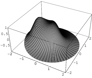
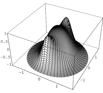
Figure 1: $k_{1}=1$ and $k_{2}=2$

Figure 2: $k_{1}=1$ and $k_{2}=3$

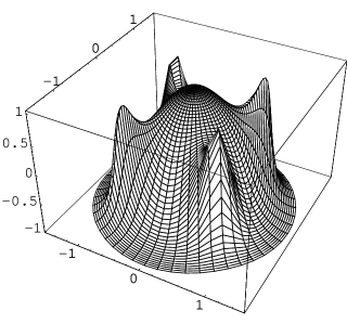
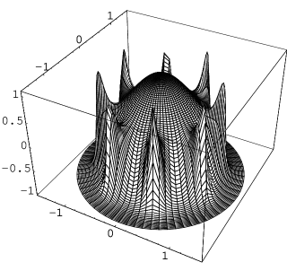
Figure 3: $k_{1}=1$ and $k_{2}=5$

Figure 4: $k_{1}=1$ and $k_{2}=9$

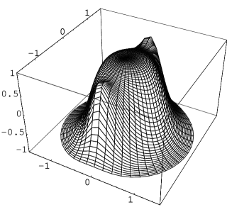
Figure 5: $k_{1}=2$ and $k_{2}=4$

For simplicity reason, we assume $\psi_{1}=\psi_{2}=0$ and $a_{1}=a_{2}=1$. We see that there is a soliton with $Q=1$ at the origin. Additionally, one, two, four or eight single satellite solitons are shown. In Fig.5 the case with $k_{1}=2$ and $k_{2}=4$ is plotted. It is very similar to Fig. 2 but now, the soliton located at the origin is ’thicker’ - it possesses $Q=2$ topological charge. One can easily continue it and find more complicated multi-soliton configurations.

It can be shown that presented configurations are also solutions of a dynamical system i.e. the well-known non-linear $O(3)$ sigma model

$$L=\frac{1}{2}(\partial_{\mu}\vec{n})^{2}.$$ (20)

This fact permits us to call the solutions of the two dimensional eikonal equation as solitons.
In order to show it we take advantage of the stereographic projection (2). Then the Lagrangian (20) takes the form

$$L=\frac{2}{(1+|u|^{2})^{2}}\partial_{\mu}u\partial^{\mu}u^{*}.$$ (21)

The pertinent equation of motion reads as follows

$$\frac{\partial_{\mu}\partial^{\mu}u}{(1+|u|^{2})^{2}}-2(\partial_{\nu}u)^{2}\frac{u^{*}}{(1+|u|^{2})^{3}}=0.$$ (22)

It is straightforward to see that it is possible to introduce a submodel defined by the following two equations: a dynamical equation

$$\partial_{\mu}\partial^{\mu}u=0$$ (23)

and a non-dynamical constrain

$$(\partial_{\nu}u)^{2}=0,$$ (24)

which is just the eikonal equation. One can notice that every solution of the submodel fulfills the field equation for the original model as well. However, it has to be underlined that the space of solutions of the original model is much larger than the restricted theory.
Inserting the Ansatz (3) into the first formula (23) we obtain

$$\sum_{j=1}^{N}e^{ik_{j}\phi}\left(\frac{1}{r}\partial_{r}(rf^{\prime}_{j})-\frac{k^{2}_{j}}{r^{2}}f_{j}\right)=0.$$ (25)

One can easily check that solutions (5) and (6) satisfy this equation. It proves that our multi-soliton configurations are not only solutions of the eikonal equation but also are generated from Lagrangian (20). Thus, we are able to calculate the corresponding energy. It is easy to see that all solutions possess finite total energy. In fact, $T_{00}$ part of the energy-momentum tensor

$$T_{00}=\frac{2\sum_{i,j=1}^{N}a_{i}a_{j}k_{i}k_{j}r^{k_{i}+k_{j}-2}\cos[(k_{i}-k_{j})\phi+(\psi_{i}-\psi_{j})]}{\left(\sum_{i,j=1}^{N}a_{i}a_{j}r^{k_{i}+k_{j}}\cos[(k_{i}-k_{j})\phi+(\psi_{i}-\psi_{j})]+1\right)^{2}}$$ (26)

does not have any point-like singularities and tends to zero for $r\rightarrow\infty$ sufficiently fast to assure finiteness of the energy.
We explicitly calculate the total energy in the case $N=2$. Using previously obtained solution we find that

$$E=2\int_{0}^{\infty}\int_{0}^{2\pi}\frac{rdrd\phi}{r^{2}}\frac{k_{1}^{2}r^{2k_{1}}+k_{2}^{2}r^{2k_{2}}+2k_{1}k_{2}r^{k_{1}+k_{2}}\cos(k_{1}-k_{2})\phi}{(1+r^{2k_{1}}+r^{2k_{2}}+2r^{k_{1}+k_{2}}\cos(k_{1}-k_{2})\phi)^{2}}.$$ (27)

This integral can be evaluated and one obtains

$$E=4\pi\mbox{max}(k_{1},k_{2}).$$ (28)

It is equivalent to the following relation

$$E=4\pi Q.$$ (29)

The multi-soliton solutions saturate the famous energy-charge inequality for $O(3)$ sigma model i.e. $E\geq 4\pi|Q|$. It means that they are stable. It is not possible to have less energy solutions with a fixed value of the total topological number. It is worth to stress that a single soliton solution with $n$ topological index has exactly the same energy as collection of $n$ solitons with an unit charge. Moreover, the energy of the multi-soliton solutions does not depend on the relative position of the solitons. It gives us the possibility to analyze scattering of the solitons using the standard moduli-space method.
As it was said before, all result presented in this section are well known. However, we have reproduce them from a new point of view i.e. using the complex eikonal equation. It is nothing surprising if we observe that the eikonal equation in the two dimensions leads to a generalization of the Cauchy-Riemann equations

$$u_{z}u_{\bar{z}}=0,$$ (30)

where $z=x+iy$. Since all Baby Skyrmions are rational functions of the $z$ variable (or $\bar{z}$) thus they can be in the natural way found in the eikonal equation.

3 $(3+1)$ dimensions: the eikonal knots

Let us now turn to the complex scalar field $u$ living in the $3+1$ dimensional Minkowski space-time. Analogously as in the previous section such a complex field can be used, via the stereographic projection, to parameterize a three component unit vector field $\vec{n}$:

$$\vec{n}=\frac{1}{1+|u|^{2}}(u+u^{*},-i(u-u^{*}),|u|^{2}-1).$$ (31)

Due to the fact that all static configurations, such that $\vec{n}\rightarrow\vec{n}_{0}=\overrightarrow{\mbox{const.}}$ for $|\vec{x}|\rightarrow\infty$, are maps $\vec{n}:R^{3}\cup\{\infty\}\rightarrow S^{2}$, can be divided into disconnected classes and characterized by a pertinent topological charge, so-called Hopf index $Q_{H}\in\pi_{3}(S^{2})$. In this section we will show how such configurations can be generated by means of the complex eikonal equation in the three space dimensions

$$\partial_{i}u\partial^{i}u=0.$$ (32)

In order to find exact solutions we assume the toroidal symmetry of the problem and introduce the toroidal coordinates

$$x=\frac{\tilde{a}}{q}\sinh\eta\cos\phi,$$

$$y=\frac{\tilde{a}}{q}\sinh\eta\sin\phi,$$

$$z=\frac{\tilde{a}}{q}\sin\xi,$$ (33)

where $q=\cosh\eta-\cos\xi$ and $\tilde{a}>0$ is a constant of dimension of length fixing the scale. Moreover, we propose a generalized version of the Aratyn-Ferreira-Zimerman-Adam Ansatz [17], [22] given by the following formula

$$u=\sum_{j=1}^{N}f_{j}(\eta)e^{i(m_{j}\xi+k_{j}\phi)}+c,$$ (34)

where $m_{i},\;k_{i}$ are integer numbers whereas $f_{i}$ are unknown real functions depending only on the $\eta$ coordinate. Additionally, $c$ is a complex number. Inserting our Ansatz (34) into the eikonal equation (32) one derives

$$0=\sum_{j=1}^{N}e^{2i(m_{j}\xi+k_{j}\phi)}\left(f^{\prime 2}_{j}-\left(m_{j}^{2}+\frac{k^{2}_{j}}{\sinh^{2}\eta}\right)f_{j}^{2}\right)+$$

$$2\sum_{j<l}e^{i((m_{j}+m_{l})\xi+(k_{j}+k_{l})\phi)}\left(f^{\prime}_{j}f^{\prime}_{l}-\left(m_{j}m_{l}+\frac{k_{j}k_{l}}{\sinh^{2}\eta}\right)f_{j}f_{l}\right).$$ (35)

Thus the unknown shape functions $f_{i}$ should obey the following equations

$$f^{\prime 2}_{j}-\left(m_{j}^{2}+\frac{k^{2}_{j}}{\sinh^{2}\eta}\right)f_{j}^{2}=0,$$ (36)

for $j=1...N$ and

$$f^{\prime}_{j}f^{\prime}_{l}-\left(m_{j}m_{l}+\frac{k_{j}k_{l}}{\sinh^{2}\eta}\right)f_{j}f_{l}=0,$$ (37)

for all $j\neq l$. The first set of the equations can be rewritten into the form

$$f^{\prime}_{j}=\pm\sqrt{\left(m_{j}^{2}+\frac{k_{j}^{2}}{\sinh^{2}\eta}\right)}f_{j}.$$ (38)

In the case of the positive sing we obtain solutions which have been originally found by Adam [22]

$$f_{j}=A_{j}\sinh^{|k_{j}|}\eta\frac{\left(|m_{j}|\cosh\eta+\sqrt{k_{j}^{2}+m_{j}^{2}\sinh^{2}\eta}\right)^{|m_{j}|}}{\left(|k_{j}|\cosh\eta+\sqrt{k_{j}^{2}+m_{j}^{2}\sinh^{2}\eta}\right)^{|k_{j}|}}.$$ (39)

They correspond to the following asymptotic value of the unit vector field

$$\vec{n}\rightarrow\frac{1}{1+|c|^{2}}(c+c^{*},-i(c-c^{*}),|c|^{2}-1)\;\;\;\mbox{as}\;\;\eta\rightarrow 0$$ (40)

and

$$\vec{n}\rightarrow(0,0,1)\;\;\;\mbox{as}\;\;\eta\rightarrow\infty.$$ (41)

For the minus sing the solutions read

$$f_{j}=\frac{B_{j}}{\sinh^{|k_{j}|}\eta}\frac{\left(|k_{j}|\cosh\eta+\sqrt{k_{j}^{2}+m_{j}^{2}\sinh^{2}\eta}\right)^{|k_{j}|}}{\left(|m_{j}|\cosh\eta+\sqrt{k_{j}^{2}+m_{j}^{2}\sinh^{2}\eta}\right)^{|m_{j}|}},$$ (42)

and the asymptotic behavior of the unit field is

$$\vec{n}\rightarrow(0,0,1)\;\;\;\mbox{as}\;\;\eta\rightarrow 0$$ (43)

and

$$\vec{n}\rightarrow\frac{1}{1+|c|^{2}}(c+c^{*},-i(c-c^{*}),|c|^{2}-1)\;\;\;\mbox{as}\;\;\eta\rightarrow\infty.$$ (44)

Let us now consider the second set of equations (37) and express constants as before i.e. $A_{j}=a_{j}e^{i\psi_{j}}$. We also take advantage of the fact that every $f_{i}$ has to fulfill equation (36). Then, inserting (38) into (37) we obtain that

$$\sqrt{\left(m_{j}^{2}+\frac{k_{j}^{2}}{\sinh^{2}\eta}\right)}\sqrt{\left(m_{l}^{2}+\frac{k_{l}^{2}}{\sinh^{2}\eta}\right)}=m_{j}m_{l}+\frac{k_{j}k_{l}}{\sinh^{2}\eta}.$$ (45)

It leads to the relation

$$m_{j}^{2}k_{l}^{2}+m_{l}^{2}k_{j}^{2}=2m_{j}m_{l}k_{j}k_{l}$$ (46)

or

$$(m_{j}k_{l}-m_{l}k_{j})^{2}=0.$$ (47)

Finally, we derive the consistency conditions relating the integer constants included in Ansatz (34)

$$\frac{m_{j}}{k_{j}}=\frac{m_{l}}{k_{l}},\;\;\;j,l=1...N$$ (48)

In other words, our Ansatz (34) is a solution of the eikonal equation (with functions $f$ given by (39) or (42)) only if the ratio between the parameters $k_{i}$ and $m_{i}$ is a constant number.
It is easy to notice that one can find more general solution of the complex eikonal equation than the Ansatz. In fact, using the simplest one-component solution with $m=k=1$

$$u_{0}=\frac{1}{\sinh\eta}e^{i(\xi+\phi)},$$ (49)

we are able to generate other solutions. It follows from the observation that any function of this solution solves the eikonal equation as well. Thus

$$u=F(u_{0}),$$ (50)

where $F$ is any reasonable function, gives a new solution [22]. Now, our Ansatz can be derived by acting a polynomial function $F$ on the fundamental solution $u_{0}$ i.e. $F(u_{0})=c_{o}+c_{1}u+...+c_{N}u^{N}$.
Calculation of the total Hopf index corresponding to the upper obtained solutions can be carried out analogously as in the two-dimensional case. Then, one obtains that

$$Q_{H}=-\mbox{max}\{k_{i}m_{i},i=1...N\}.$$ (51)

Of course, it can be also found directly by calculation how many times the vector field $\vec{n}$ wraps in the angular directions. For $N=1$ and $c_{0}=0$ we see that $\vec{n}$ wraps $m$ times around $\xi$-direction and $k$ times around $\phi$-direction, giving $Q_{H}=-mk$. One can also see that for a non-vanishing $c$ (but still for the one-knot configuration) the vector field behaves identically. Thus, the topological charge is still $Q_{H}=-mk$. For the multi-knot case, one has to not only add topological charges of the elementary hopfions but also take into account the linking number. As we discuss it in the next subsection, it leads to the same total Hopf index i.e. $Q_{H}=-mk$. Analogous calculations can be carried in the case of $N=2$.
It is worth to stress that analogously to the winding number in the $O(3)$ sigma model in $(2+1)$ dimensions, the total Hopf index is fixed by the asymptotically leading term in our Ansatz. The other components of the Ansatz affect only the local topological structure of the solution.
The position of the solution can be easily found if we recall that in the core of a knot the vector field takes the opposite value than at the spatial infinity

$$\vec{n}_{0}=-\vec{n}^{\infty},$$ (52)

where

$$\vec{n}^{\infty}=\lim_{\vec{x}\rightarrow\infty}\vec{n}=\lim_{\eta\rightarrow 0}\vec{n}.$$ (53)

Then a knotted solution is represented by a curve corresponding to $\vec{n}=\vec{n}_{0}$.
In further considerations we take solution (42), for which $f\rightarrow\infty$ as $\eta\rightarrow 0$ and $\vec{n}^{\infty}=(0,0,1)$. Thus the core of a knot is located at $\vec{n}_{0}=(0,0,-1)$. Therefore, it is given by a curve being a solution to the equation

$$\sum_{i,j=1}^{N}a_{i}a_{j}g_{i}g_{j}\cos[(m_{i}-m_{j})\xi+(k_{i}-k_{j})\phi+(\psi_{i}-\psi_{j})]+$$

$$2c_{0}\sum_{i=1}^{N}a_{i}g_{i}\cos[m_{i}\xi+k_{i}\phi+(\psi_{1}-\psi_{2})+\alpha_{0}]+c_{0}^{2}=0,$$ (54)

where $f_{i}(\eta)=A_{i}g_{i}(\eta)$ and $c=c_{0}e^{i\alpha_{0}}$. The simplest but sufficiently interesting cases with $N=1$ as well as $N=2$ are analyzed below.

3.1 N=1 case

For $N=1$ the last equation can be rewritten in the following form

$$a^{2}g^{2}+2c_{0}ag\cos[m\xi+k\phi+\psi+\alpha_{0}]+c_{0}^{2}=0.$$ (55)

Thus, knots are located at

$$g(\eta_{0})=\frac{c_{0}}{a},\;\;\;m\xi+k\phi=\pi-\psi-\alpha_{0}+2\pi l,\;\;\;l=0,1...L-1.$$ (56)

Figure 6: $m=k=1$ and $m=k=2$

Figure 7: $m=k=3$ and $m=k=4$

Due to the fact that $g$ is the monotonic function from $\infty$ to $0$, there is exactly one $\eta_{0}$ satisfies upper condition. Thus, obtained configuration is given by a closed curve (or curves) (56) wrapped on a torus $\eta=\eta_{0}$. In general, for fixed values of the parameters $m,k$ one finds that the number $L$ of the elementary knots is equal to the greatest common divisor $m$ and $k$. The whole multi-knot solution is a collection of such elementary knots which are linked together. Of course, every elementary knot should be treated in the same manner as others so they all carry the identical topological charge $Q_{e}=-pq$, where $p,q$ are relative prime numbers and $\frac{m}{k}=\frac{p}{q}$. We immediately see that simple sum of all charges of elementary knots is not equal to the total topological number $Q=-km$. In order to correctly calculate the topological charge one has to take into account the linking number $N_{L}$ between elementary knots as well. Finally, we derive that

$$Q_{H}=K\cdot Q_{e}-N_{L}.$$ (57)

Correctness of this formula will be checked in some (but sufficiently general) cases.

Figure 8: $m=1,k=2$ and $m=1,k=3$

Figure 9: $m=1,k=4$ and $m=1,k=5$

Figure 10: $m=2,k=4$ with elementary knots

Let us discus some of the obtained multi-knot configurations in details. For simplicity we assume $\psi_{1}=\psi_{2}=0$, $a_{1}=a_{2}=1$. In Fig. 6 the simplest eikonal knot with $m=k=1$ is presented. The position of the knot is given by a circle and this configuration possesses toroidal symmetry. In the same figure the case with $m=k=2$ is demonstrated as well. As one could expect such a configuration consists of two elementary knots with $Q_{e}=-1$ (circles) which are linked together. The linking number is $N_{L}=2$ so this configuration has the total charge $Q=-4$, what is in accordance with the formula (57). Other multi-knot configurations built of the elementary knots with $Q_{e}=-1$ are plotted in Fig. 7 ($m=k=3$ and $m=k=4$). One can easily check that (57) is fulfilled as well.
The more sophisticated case is shown in Fig. 8, where a single knot solution for $m=1,k=2$ as well as for $m=1,k=3$ is presented. In contradistinction to the previously discussed knot this configuration does not have the toroidal symmetry (of course, one can easily restore the toroidal symmetry by setting $c=0$). In Fig. 9 further examples with $m=1,k=4$ and $m=1,k=5$ are shown. Now, it is obvious how this type of knots (i.e. with $R\equiv\frac{k}{m}\in\mathcal{N}$) looks like. They cross $2R$ times the $xy$-plane, or in the other words they wrap $R$ times ’vertically’ on the torus $\eta_{0}$.

Figure 11: $m=1,k=70$

Figure 12: $m=2,k=1$ and $m=3,k=1$

Figure 13: $m=4,k=1$ and $m=5,k=1$

Figure 14: $m=4,k=2$ with elementary knots

Figure 15: $m=70,k=1$

Figure 16: $m=2,k=3$ and $m=3,k=2$

Figure 17: $m=2,k=5$ and $m=3,k=4$

Figure 18: $m=30,k=17$

Another configuration with two elementary knots is presented in Fig. 10. Also in this case relation (57) is satisfied - the corresponding linking number is $N_{L}=4$ and $Q_{e}=-2$. In Fig. 11 a knot with $m=1,k=70$ is plotted. It is clearly visible that the knot is situated on a torus. Another simple type of solutions can be obtained for $\frac{1}{R}\in N$. Such knots with $m=2,k=1$ and $m=3,k=1$ are shown in Fig. 12. Here, the knot wraps $R$ times but in the ’horizontal’ direction on the torus i.e. around $z$-axis. Knots with higher topological charges ($m=4,k=1$ and $m=5,k=1$) are plotted in Fig. 13. In Fig. 14 the simplest two-knot configuration of this type is demonstrated whereas in Fig 15 one can find a solution with $m=70,n=1$. It is straightforward to notice that, in spite of the fact that upper discussed knots belong to distinct topological classes, the curves describing their position are topological equivalent to a simple circle.
More complicated and really knotted configurations have been found for $R=\frac{p}{q}$, where $p,q$ are relative prime numbers distinct from one. The simplest trefoil knots with $R=3/2$ and $R=2/3$ are presented in Fig. 16. In both cases the Hopf charge is $Q_{H}=-6$. In Fig. 17 farther examples of knots with $R=2/5$ as well as $R=3/4$ are plotted. In Fig. 18 a really highly knotted solution with $Q_{H}=-510$ is presented. We see that any Hopf solution with $R=\frac{p}{q}$ wraps simultaneously $q$ times around $z$-axis and $p$ times around circle $\eta=\infty$.

3.2 N=2 case

Let us now consider the second simple case i.e. we take $N=2$ and put $c=0$. It enables us to construct a new class of multi-knot configurations which differ from previously described. Equation (54) takes the form

$$0=a_{1}^{2}g_{1}^{2}+a_{2}^{2}g_{2}^{2}+2a_{1}a_{2}g_{1}g_{2}\cos[(m_{1}-m_{2})\xi+(k_{1}-k_{2})\phi+(\psi_{1}-\psi_{2})].$$ (58)

One can solve it and obtain the position of knots. In this case we can distinguish two sorts of solutions. Namely, a central knot located at

$$\eta=\infty$$

Figure 19: $m_{1}=k_{1}=1$, $m_{2}=k_{2}=2$ and $m_{1}=k_{1}=1$, $m_{2}=k_{2}=3$

and satellite knots

$$\frac{g_{1}}{g_{2}}=\frac{a_{2}}{a_{2}},\;\;\;\;\;(m_{1}-m_{2})\xi+(k_{1}-k_{2})\phi=\pi-(\psi_{1}-\psi_{2})+2l\pi,$$ (59)

where $l=0,...|L_{1}-L_{2}|-1$. It should be notice that the condition $\frac{g_{1}}{g_{2}}=\frac{a_{2}}{a_{2}}$ can be always satisfied. It is due to the fact that $g_{1}/g_{2}$ is a function smoothly and monotonically interpolating between $\infty$ and $0$ (of course if $k_{1}\neq k_{2})$. From (59) we find that for a fixed value of the parameters $m_{i},k_{i}$ there are $|L_{1}-L_{2}|$ knots: one in $\eta=\infty$ (circle) and $|L_{1}-L_{2}|-1$ satellite knots (loops) which can take various, quite complicated and topologically inequivalent shapes. Additionally, one can observe that the Hopf index of the central knot is $Q_{c}=-\mbox{min}\{k_{i}m_{i},i=1..N\}$.

Figure 20: $m_{1}=2,k_{1}=4$, $m_{2}=1,k_{2}=2;$ $m_{1}=2,k_{1}=6$, $m_{2}=1,k_{2}=3$

Figure 21: $m_{1}=4,k_{1}=2$, $m_{2}=2,k_{2}=1;$ $m_{1}=4,k_{1}=6$, $m_{2}=2,k_{2}=3$

In Fig. 19 the simplest types of solutions, with $m_{1}=k_{1}=1$, $m_{2}=k_{2}=2$ and $m_{1}=k_{1}=1$, $m_{2}=k_{2}=3$ are demonstrated. We see that they are very similar to the corresponding solutions with $N=1$ (see Fig. 6 and Fig. 7). More complicated situations are plotted in Fig. 20 and Fig. 21. In all configurations the central knot is clearly visible as a circle around origin, whereas knots known form the previous subsection wrap around this central knot.

It is obvious to notice that presented solutions (even one-knot configurations) do not possess toroidal symmetry. Surfaces of a constant value of the third component $n^{3}$ are not (in general) toruses. In this manner they differ profoundly from the standard knotted soliton configurations previously presented in the literature [16], [17], [19]. Here, the position of a knot depends on a (constant) value of the radial coordinate $\eta$ as well as on the angular coordinates $\xi,\,\phi$. Up to our best knowledge non-toroidal knots have been not, in the exact form, presented in the literature yet.
One has to be aware that all knots found in this paper are solutions of the complex eikonal equation only. It is not known any Lagrangian which would give these multi-knot configurations as solutions of the pertinent equations of motion. They differ from toroidal solitons obtained recently in the Aratyn-Ferreira-Zimerman (and its generalizations) and the Nicole model. However, it is worth to notice that the simplest one knot state with $k=m=1$

$$u(\eta,\xi,\phi)=\frac{1}{\sinh\eta}e^{i(\xi+\phi)}$$ (60)

is identical to the soliton with $Q_{H}=-1$ obtained in these models [16], [17]. As we do not know the form of the Lagrangian we are not able to calculate the energy corresponding to the obtained multi-knot solutions. Thus, their stability and saturation of the Vakulenko-Kapitansky inequality [23] are still open problems.

4 The eikonal knots and the Faddeev-Niemi hopfions

In spite of the upper mentioned problems our multi-knot configurations become more physically interesting, and potentially can have realistic applications, if one analyzes them in the connection with the Faddeev-Skyrme-Niemi effective model of the low energy gluodynamics

$$L=\frac{1}{2}m^{2}(\partial_{\mu}\vec{n})^{2}-\frac{1}{4e^{2}}[\vec{n}\cdot(\partial_{\mu}\vec{n}\times\partial_{\nu}\vec{n})]^{2}.$$ (61)

It is straightforward to see that all finite energy solutions in this model must tend to a constant $\vec{n}_{\infty}$ at the spatial infinity. Then field configurations being maps from $S^{3}$ into $S^{2}$ can be divided into disconnected classes and characterized by the Hopf index. Indeed, many configurations with a non-trivial topological charge, which appear to form knotted structures have been numerically obtained [13], [14].
In order to reveal a close connection between the eikonal knots and Faddeev-Niemi hopfions we rewrite the equations of motion for model (61) in terms of the complex field $u$ (31) [17]

$$(1+|u|^{2})\partial^{\mu}L_{\mu}-2u^{*}(L^{\mu}\partial_{\mu}u)=0$$ (62)

where

$$L_{\mu}=m^{2}\partial_{\mu}u-\frac{4}{e^{2}}\frac{K_{\mu}}{(1+|u|^{2})^{2}}$$

$$K_{\mu}=(\partial^{\nu}u\partial_{\nu}u^{*})\partial_{\mu}u-(\partial^{\nu}u)^{2}\partial_{\mu}u^{*}.$$ (63)

It has been recently observed [17] that such a model possesses an integrable submodel if the following constrain is satisfied

$$L_{\mu}\partial^{\mu}u=0.$$ (64)

Then, infinite family of the local conserved currents can be constructed [24], [25], [26], [27]. On the other hand, it is a well-known fact from the standard $(1+1)$ and $(2+1)$ soliton theory that the existence of such a family of the currents usually leads to soliton solutions with a non-trivial topology. Due to that one should check whether also in the case of the Faddeev-Skyrme-Niemi model the integrability condition can give us some hints how to construct knotted solitons.
For model (61) the integrability condition takes the form

$$m^{2}(\partial_{\nu}u)^{2}=0.$$ (65)

It vanishes if mass is equal to zero or the eikonal equation is fulfilled. The first possibility is trivial since $m=0$ means the absence of the kinetic term in Lagrangian (61) and no stable soliton solutions can be obtained due to the instability under the scale transformation. Thus, the eikonal equation appears to be the unique, nontrivial integrability condition for the Faddeev-Skyrme-Niemi model.
However, it should be stressed that the full integrable submodel consists of two equations. Namely, apart from the integrability condition (64), also the dynamical equation has to be taken into account

$$\partial_{\mu}\left[m^{2}\partial_{\mu}u-\frac{4}{e^{2}}\frac{\partial^{\nu}u\partial_{\nu}u^{*}}{(1+|u|^{2})^{2}}\partial_{\mu}u\right]=0.$$ (66)

The correct solutions of the Faddeev-Skyrme-Niemi model have to satisfy both equations. Unfortunately, derived eikonal hopfions do not solve the dynamical equation and in the consequence are not solutions of the Faddeev-Skyrme-Niemi model. Nonetheless, the fact that they appear in a very natural way in the context of the Faddeev-Skyrme-Niemi model i.e. just as solutions of the integrability condition might indicate a close relation between them and the Faddeev-Niemi hopfions.
This idea seems to be more realistic if we compare the eikonal hopfions with the numerically found Faddeev-Niemi hopfions [13], [14]. It is striking that every hopfions possesses its eikonal counterpart with the same topology and a very similar shape.
Moreover, there is an additional argument which strongly supports the idea that the eikonal knots might applied in construction of approximated Faddeev-Niemi hopfions. It follows from the observation that the eikonal knots, if inserted into the total energy integral calculated for the Faddeev-Skyrme-Niemi model, give the finite value of this integral. The situation is even better. The lowest energy eikonal configurations are only approximately 20% heavier than numerically derived hopfions. Let us show it for $N=1$ Ansatz.
Indeed, the Faddeev-Skyrme-Niemi model gives, for static configurations, the following total energy integral

$$E=2m^{2}\int d^{3}x\frac{\nabla u\nabla u^{*}}{(1+|u|^{2})^{2}}+\frac{2}{e^{2}}\int d^{3}x\frac{(\nabla u\nabla u^{*})^{2}-(\nabla u)^{2}(\nabla u^{*})^{2}}{(1+|u|^{2})^{4}},$$ (67)

where the stereographic projection (31) has been taken into account. Moreover, as our solutions fulfill the eikonal equations

$$(\nabla u)^{2}=0,$$ (68)

thus

$$E=2m^{2}\int d^{3}x\frac{\nabla u\nabla u^{*}}{(1+|u|^{2})^{2}}+\frac{2}{e^{2}}\int d^{3}x\frac{(\nabla u\nabla u^{*})^{2}}{(1+|u|^{2})^{4}}.$$ (69)

Now, we can take advantage of the eikonal hopfions and substitute them into the total energy integral (69). Let us notice that

$$\nabla u\nabla u^{*}=\frac{q^{2}}{\tilde{a}^{2}}\left[f^{\prime 2}+\left(m^{2}+\frac{k^{2}}{\sinh^{2}\eta}\right)f^{2}\right]=$$

$$=2\frac{q^{2}}{\tilde{a}^{2}}\left(m^{2}+\frac{k^{2}}{\sinh^{2}\eta}\right)f^{2}$$ (70)

and the Jacobian

$$d^{3}x=\frac{\tilde{a}^{3}\sinh\eta}{q^{3}}d\xi d\phi d\eta.$$ (71)

Then

$$E=2m^{2}\tilde{a}I_{1}+\frac{2}{\tilde{a}e^{2}}I_{2},$$ (72)

where

$$I_{1}=2a^{2}\int_{0}^{\infty}d\eta\int_{0}^{2\pi}\frac{d\xi}{q}\int_{0}^{2\pi}d\phi\frac{\sinh\eta g^{2}\left(m^{2}+\frac{k^{2}}{\sinh^{2}\eta}\right)}{(1+c_{0}^{2}+a^{2}g^{2}+2ac_{0}g\cos[m\xi+k\phi])^{2}}$$ (73)

and

$$I_{2}=4a^{4}\int_{0}^{\infty}d\eta\int_{0}^{2\pi}d\xi q\int_{0}^{2\pi}d\phi\frac{\sinh\eta g^{4}\left(m^{2}+\frac{k^{2}}{\sinh^{2}\eta}\right)^{2}}{(1+c_{0}^{2}+a^{2}g^{2}+2ac_{0}g\cos[m\xi+k\phi])^{4}}.$$ (74)

As it was mentioned before we not only prove that the eikonal knots provide finiteness of the total energy but additionally we find the lowest energy configuration for fixed $k,m$. This minimization procedure should be done with respect to three (in the case of $N=1$) parameters: $\tilde{a}$ and $a,c_{0}$. At the beginning we get rid of the scale parameter $\tilde{a}$

$$\frac{\partial E}{\partial\tilde{a}}=0\;\;\Rightarrow\;\;\tilde{a}=\frac{1}{em}\sqrt{\frac{I_{2}}{I_{1}}}.$$

Then the total energy takes the form

$$E=4\frac{m}{e}\sqrt{I_{1}I_{2}}.$$ (75)

Now, we calculate the previously defined integrals. It can be carried out if one observes that

$$\int_{0}^{2\pi}\frac{d\phi}{(\alpha+\beta\cos[m\xi+k\phi])^{2}}=\frac{2\pi\alpha}{(\alpha^{2}-\beta^{2})^{\frac{3}{2}}},$$ (76)

$$\int_{0}^{2\pi}\frac{d\phi}{(\alpha+\beta\cos[m\xi+k\phi])^{4}}=\frac{\pi\alpha(2\alpha^{2}+3\beta^{2})}{(\alpha^{2}-\beta^{2})^{\frac{7}{2}}},$$ (77)

$$\int_{0}^{2\pi}\frac{d\xi}{\cosh\eta-\cos\xi}=\frac{2\pi}{\sinh\eta},$$ (78)

$$\int_{0}^{2\pi}d\xi(\cosh\eta-\cos\xi)=2\pi\cosh\eta.$$ (79)

Thus, one can finally obtain that

$$I_{1}=2a^{2}(2\pi)^{2}\int_{0}^{\infty}d\eta g^{2}\left(m^{2}+\frac{k^{2}}{\sinh^{2}\eta}\right)\frac{1+c_{0}^{2}+a^{2}g^{2}}{\left[(1+c_{0}^{2}+a^{2}g^{2})^{2}-4c_{0}^{2}a^{2}g^{2}\right]^{\frac{3}{2}}}$$ (80)

and

$$I_{2}=4a^{4}(2\pi)^{2}\int_{0}^{\infty}d\eta\sinh\eta\cosh\eta g^{4}\left(m^{2}+\frac{k^{2}}{\sinh^{2}\eta}\right)^{2}\;\times$$

$$\frac{(1+c_{0}^{2}+a^{2}g^{2})[(1+c_{0}^{2}+a^{2}g^{2})^{2}+6c_{0}^{2}a^{2}g^{2}]}{\left[(1+c_{0}^{2}+a^{2}g^{2})^{2}-4c_{0}^{2}a^{2}g^{2}\right]^{\frac{7}{2}}}$$ (81)

type of a knot $(m,n)$	$a$	$c_{0}$	$E_{min}$	$E_{num}$
(1,1)	1.252	0	304.3	252.0
(1,2)	0.357	0	467.9	417.5
(2,1)	5.23	0	602.7	417.5
(1,3)	0.065	0	658.1	578.5
(2,3)	0.3	0	1257.0	990.5

Table 1: Minimal energy of the eikonal knots and Faddeev-Niemi hopfions

type of a knot $(m,n)$	$a$	$c_{0}$	$E$
(1,1)	1.252	0.2	311.2
(1,2)	0.357	0.1	471.9
(2,1)	5.23	0.2	622.3
(1,3)	0.065	0.05	659.5
(2,3)	0.3	0.1	1269.0

Table 2: Energy of the knotted eikonal knots

It may be easily checked that these two integrals are finite for all possible profile functions of the eikonal hopfions.
Now we are able to find the minimum of the total energy (75) as a function of $a,c_{0}$. It has been done by means of numerical methods. The results $E_{min}$ for the simplest knots are presented in Table 1 (we assume $m/e=1$). Let us shortly comment obtained results.
Firstly, we see that the eikonal knots are ’heavier’ than knotted solitons found in the numerical simulations $E_{num}$ [13]. It is nothing surprising as the eikonal knots do not fulfill the Faddeev-Skyrme-Niemi equations of motion that is do not minimize the pertinent action. However, the difference is small and is more less equal 20% . Strictly speaking the accuracy varies from 15% for the lightest knots with $m=1$ up to 30-35% in the case of knots with bigger value of $Q_{H}$ or $m$ parameter. This result is really unexpected since the eikonal knots are solutions of such a very simple (first order and almost linear) equation.
Secondly, the lowest energy configurations are achieved for $c_{0}=0$. As we know it means that a knot is located at $\eta_{0}=\infty$. In other words, for fixed $m,k$ the unknot (i.e. configurations where surfaces $n^{3}=const.$ are toruses) possesses lower energy than other knotted eikonal solutions. It is a little bit discouraging since the Faddeev-Niemi hopfions are in general really knotted solitons. However, one can observe that even very small increase of the energy $E$ causes that $c_{0}\neq 0$ (see Table 2). Then, what is more important, also the ratio $\frac{c_{0}}{a}$ differs from zero significantly. It guarantees that the knotted structure of a eikonal solution becomes restored.
Thirdly, there is no $m\leftrightarrow k$ degeneracy. The eikonal knots with $m=p,k=q$ and $m=q,k=p$ do not lead to the same total energy. In particular, for configurations with the fixed topological charge, the lowest energy state is a knot with $m=1$. In the case of knots with bigger value of the parameter $m$ the total energy grows significantly.
We see that the eikonal knots seem to be quite promising and can be applied to the Faddeev-Skyrme-Niemi model. Since our solutions possess a well defined topological charge and approximate the shape as well as the total energy of the Faddeev-Niemi hopfions with on an average 20% accuracy, one could regard them as first step in construction of approximated solutions (given by the analytical expression) to the Faddeev-Skyrme-Niemi model.
Recently Ward [28] has analyzed the instanton approximations to Faddeev-Niemi hopfions with $Q_{H}=1,2$ Hopf index. It would be very interesting to relate it with the eikonal approximation.
It should be noticed that similar construction provides approximated, analytical solutions in non-exactly solvable $(2+1)$ dimensional systems. In fact, the Baby Skyrme model [29] and Skyrme model in $(3+1)$ dimensions [30], [31] can serve as very good examples.

5 Conclusions

In this work multi-soliton and multi-knot configurations, generated by the eikonal equation in two and three space dimensions respectively, have been discussed. It has been proved that various topologically non-trivial configurations can be systematically and analytically derived from the eikonal equation.
In the model with the two space dimensions (which is treated here just as a toy model for the later investigations) multi-soliton solutions corresponding to the $O(3)$ sigma model have been obtained. In particular, we took under consideration one and two component Ansatz i.e. $N=1,2$. In this case we restored the standard result that the energy of a multi-soliton solution depends only on the total topological number. The way how the topological charge is distributed on the individual solitons does not play any role. Thus, for example, the energy of a single soliton with winding number $n$ is equal to the energy of a collection of $n$ solitons with the unit charge. In both cases we observe saturation of the energy-charge inequality. Moreover, energy remains constant under any changes of positions of the solitons. It is exactly as in the Bogomolny limit where topological solitons do not attract or repel each other. Due to that the whole moduli space has been found.
In the most important, three dimensional space case we have found that the eikonal equation generates multi-knot configurations with an arbitrary value of the Hopf index. As previously, Ansatz (34) with one and two components has been investigated in details. Let us summarize obtained results.
Using the simplest, one component Ansatz (34) we are able to construct one as well as multi-knot configurations which, in general, consist of the same (topologically) knots linked together. The elementary knot can have various topology. For example a trefoil knot has been derived. It is unlikely the standard analytical hopfion solutions which have always toroidal symmetry and are not able to describe such a trefoil state.
By means of the two component Ansatz multi-knot configurations with a central knot located at $\eta=\infty$ and a few satellite knots winded on a torus $\eta=const$ have been obtained. In the contrary to the central knot, which is always circle, satellite solitons can take various, topologically inequivalent shapes known from the $N=1$ case.
In addition, we have argued that the multi-knot solutions can be useful in the context of the Faddeev-Skyrme-Niemi model. Thus, they appear to be interesting not only from the mathematical point of view (as analytical knots) but might also have practical applications. We have shown that the eikonal knots provide an analytical framework in which the qualitative features of the Faddeev-Niemi hopfions can be captured. Moreover, also quantitative aspects i.e. the energy of the hopfion can be investigated as well. Although the eikonal knots are approximately 20% heavier than the numerical hopfions, what is rather a poor accuracy in compare with the rational Ansatz for Skyrmions, one can expect that for other shape functions a better approximation might be obtained.
There are several directions in which the present work can be continued. First of all one should try to achieve better approximation to the knotted solutions of the Faddeev-Skyrme-Niemi effective model. It means that new, more accurate shape functions have to be checked. It is in accordance with the observation that presented here knots solve only the integrability condition (eikonal equation) but not the pertinent dynamical equations of motion. Due to that it is not surprising that the eikonal shape function is an origin for some problems (eikonal knots are too heavy and tend to unknotted configurations). One can expect that these new shape functions will not only better approximate the energy of the Faddeev-Niemi hopfions but also guarantee non-zero value of the parameter $c_{0}$ and ensure the knotted structure of the solutions. We would like to address this issue in our next paper.
There is also a very interesting question concerning the shape of the eikonal hopfions. Cores of all presented here knots are situated on a torus with a constant radius. However, there are many knots which cannot be plotted as a closed curve on a torus. Thus one could ask whether it is possible to construct such knots (non-torus knots) in the framework of the eikonal equation.
Of course, one might also apply the eikonal equation to face more advanced problems in the Faddeev-Skyrme-Niemi theory and investigate time-dependent configurations as for instance scattering solutions or breather.
On the other hand, one can try to find a Lagrangian which possesses obtained here topological configurations as solutions of the corresponding field equations. One can for example consider recently proposed modifications of the Faddeev-Skyrme-Niemi model which break the global $O(3)$ symmetry [32], [33], [34]. Application of the eikonal equation to other models of glueballs [35], [36], based in general on the $\vec{n}$ field, would be also interesting.

I would like to thank Prof. A. Niemi for discussion. I am also indebted to Dr. C. Adam and Prof. H. Arodź for many valuable and helpful remarks.
This work is partially supported by Foundation for Polish Science FNP and ESF ”COSLAB” programme.

References

- [1] T. T. Wu and C. N. Yang, in Properties of Matter Under Unusual Conditions, edited by H. Mark, S. Fernbach (Interscience, New York, 1969).
- [2] G. ’t Hooft, Nucl. Phys. B 79, 276 (1974); G. ’t Hooft, Nucl. Phys. B 153, 141 (1979); A. Polyakov, Nucl. Phys. B 120, 429 (1977).
- [3] A. Vilenkin and P. E. S. Shellard, Cosmic Strings and Other Topological Defects, Cambridge Uviversity Press, (2000); M. B. Hindmarsh and T. W. Kibble, Rept. Prog. Phys. 58, 477 (1995); T. W. Kibble, Acta Phys. Pol. B 13, 723 (1982); T. W. Kibble, Phys. Rep. 67, 183 (1980); W. H. Żurek, Nature 317, 505 (1985).
- [4] T. W. Kibble in Patterns of Symmetry Breaking edited by H. Arodź, J. Dziarmaga, W. H. Żurek, NATO Science Series (2003); M. Sakallariadou ibidem; A. C. Davis ibidem.
- [5] G. E. Volovik, Exotic Properties of Superfluid , World Scientific, Singapore (1992).
- [6] R. J. Donnelly, Quantized Vortices in Helium II, Cambridge University Press (1991).
- [7] L. Faddeev, in 40 Years in Mathematical Physics, World Scientific, Singapore (1995).
- [8] L. Faddeev and A. Niemi, Nature 387, 58 (1997); L. Faddeev and A. Niemi, Phys. Rev. Lett. 82, 1624 (1999); E. Langmann and A. Niemi, Phys.Lett. B 463, 252 (1999).
- [9] Y. M. Cho, Phys. Rev.D 21, 1080 (1980); Y. M. Cho, Phys. Rev. D 23, 2415 (1981); Y. M. Cho, Phys. Rev. Lett. 46, 302 (1981); Y. M. Cho, Phys. Rev. Lett. 87, 252001 (2001); Y. M. Cho, H. W. Lee and D. G. Pak, Phys. Lett. B 525, 347 (2002); W. S. Bae, Y. M. Cho and S. W. Kimm, Phys. Rev. D 65, 025005 (2002); Y. M. Cho, Phys. Lett. B 603, 88 (2004).
- [10] S. V. Shabanov, Phys. Lett. B 463, 263 (1999); S. V. Shabanov, Phys. Lett. B 458, 322 (1999);
- [11] K.-I. Kondo, T. Murakami and T. Shinohara, hep-th/0504107; K.-I. Kondo, Phys. Lett. B 600, 287 (2004).
- [12] J. Gladikowski and M. Hellmund, Phys. Rev. D 56, 5194 (1997).
- [13] R. A. Battye and P. M. Sutcliffe, Phys. Rev. Lett. 81, 4798 (1998); R. A. Battye and P. M. Sutcliffe, Proc.Roy.Soc.Lond. A 455, 4305 (1999).
- [14] J. Hietarinta and P. Salo, Phys. Lett. B 451, 60 (1999); J. Hietarinta and P. Salo, Phys. Rev. D 62, 81701 (2000).
- [15] R. S. Ward, Phys.Lett.B 473, 291 (2000); R. S. Ward, Nonlinearity 12, 241 (1999); R. S. Ward, Phys. Rev. D 70, 061701 (2004).
- [16] D. A. Nicole, J. Phys. G 4 , 1363 (1978).
- [17] H. Aratyn, L. A. Ferreira and A. H. Zimerman, Phys. Lett. B 456, 162 (1999); H. Aratyn, L. A. Ferreira and A. H. Zimerman, Phys. Rev. Lett. 83, 1723 (1999).
- [18] A. Wereszczyński, Eur. Phys. J. C 38, 261 (2004).
- [19] A. Wereszczyński, Mod. Phys. Lett. A 19, 2569 (2004); A. Wereszczyński, Acta Phys. Pol. B 35, 2367 (2004).
- [20] G. H. Derrick, J. Math. Phys. 5, 1252 (1964).
- [21] S. Deser, M. J. Duff and C. J. Isham, Nucl. Phys. B 114, 29 (1977).
- [22] C. Adam, J. Math. Phys. 45, 4017 (2004).
- [23] A. F. Vakulenko and L. V. Kapitansky, Sov. Phys. Dokl. 24, 432 (1979).
- [24] O. Alvarez, L. A. Ferreira and J. Sánchez-Guillén, Nucl. Phys. B 529, 689 (1998).
- [25] O. Babelon and L. A. Ferreira, JHEP 0211, 020 (2002).
- [26] J. Sánchez-Guillén, Phys.Lett. B 548, 252 (2002), Erratum-ibid. B 550, 220 (2002); J. Sánchez-Guillén and L. A. Ferreira, in ”Sao Paulo 2002, Integrable theories, solitons and duality” unesp2002/033, hep-th/0211277.
- [27] C. Adam and J. Sánchez-Guillén, J.Math.Phys. 44, 5243 (2003).
- [28] R. S. Ward, Nonlinearity 14, 1543 (2001).
- [29] A. E. Kudryavtsev, B. M. A. G. Piette and W. J. Zakrzewski, Nonlinearity 11, 783 (1998); T. I. Ioannidou, V. B. Kopeliovich and W. J. Zakrzewski, JHEP 95, 572 (2002).
- [30] T. H. R. Skyrme, Proc. Roy. Soc. Lon. 260, 127 (1961).
- [31] R. A. Battye and P. M. Sutcliffe, Phys. Rev. Lett. 79, 363 (1997); C. J. Houghton, N. S. Manton and P. Sutcliffe, Nucl. Phys. B 510, 507 (1998).
- [32] L. Faddeev and A. Niemi, Phys. Lett. B 525, 195 (2002).
- [33] L. Dittmann, T. Heinzl and A. Wipf, Nucl. Phys. B (Proc. Suppl.) 106, 649 (2002); L. Dittmann, T. Heinzl and A. Wipf, Nucl. Phys. B (Proc. Suppl.) 108, 63 (2002).
- [34] A. Wereszczyński and M. Ślusarczyk, Eur. Phys. J. C 39, 185 (2005).
- [35] V. Dzhunushaliev, D. Singleton and T. Nikulicheva, hep-ph/0402205; V. Dzhunushaliev, hep-ph/0312289.
- [36] D. Bazeia, M. J. dod Santos and R. F. Ribeiro, Phys. Lett. A 18, 84 (1995).