Abstract

We study a class of oscillating bounce solutions to the Euclidean field equations for gravity coupled to a scalar field theory with two, possibly degenerate, vacua. In these solutions the scalar field crosses the top of the potential barrier $k>1$ times. Using analytic and numerical methods, we examine how the maximum allowed value of $k$ depends on the parameters of the theory. For a wide class of potentials $k_{\rm max}$ is determined by the value of the second derivative of the scalar field potential at the top of the barrier. However, in other cases, such as potentials with relatively flat barriers, the determining parameter appears instead to be the value of this second derivative averaged over the width of the barrier. As a byproduct, we gain additional insight into the conditions under which a Coleman-De Luccia bounce exists. We discuss the physical interpretation of these solutions and their implications for vacuum tunneling transitions in de Sitter spacetime.

I Introduction

There has recently been renewed interest in the problem of vacuum tunneling in de Sitter spacetime. Although this interest has been sparked in large part by developments in string theory, the tunneling problem itself can be addressed within the context of quantum field theory. The essence of the problem is captured by considering a theory with a single scalar field described by the Lagrangian

$${\cal L}={1\over 2}(\partial_{\mu}\phi)^{2}-V(\phi)$$ (1)

where the scalar field potential has two unequal minima, as illustrated in Fig. 1. The lower minimum corresponds to the stable “true vacuum” state, while the higher minimum corresponds to a metastable “false vacuum”.

At zero temperature, and in the absence of gravitational effects, the false vacuum decays via a quantum mechanical tunneling process that leads to the nucleation of bubbles of true vacuum. The semiclassical calculation of the bubble nucleation rate per unit volume, $\Gamma$, is well understood [1, 2]. It can be written in the form

$$\Gamma=Ae^{-B}$$ (2)

where $B$ is obtained from the action of the “bounce” solution to the Euclideanized field equations. This bounce solution has a region of approximate true vacuum (essentially, a four-dimensional bubble) separated by a wall region from a false vacuum exterior.

FIG. 1.: The potential for a typical theory with a false vacuum.

At finite temperature, bubble nucleation proceeds via both quantum tunneling and thermal fluctuations. When the temperature $T$ is high enough that the latter process dominates, $\Gamma$ can still be written in the form of Eq. (2), but with $B=E/T$, where $E$ is the energy of a critical bubble.

In this paper we will be concerned with vacuum tunneling in situations where gravitational effects are important. We will assume that $V(\phi)>0$ everywhere, so that both the false and true vacua correspond to de Sitter spacetimes. This problem was first discussed by Coleman and De Luccia [3], who argued that the proper generalization of the flat spacetime calculation of $B$ could be obtained by looking for a bounce solution of the Euclidean version of the coupled matter plus gravity field equations. When the relevant mass scales are well below the Planck mass and the bubble sizes are small compared to the curvature of the de Sitter space, the Coleman-De Luccia prescription leads to a description of bubble nucleation that is very similar to that of the zero-temperature flat spacetime case, with small gravitational corrections of the expected order of magnitude.

However, when the mass scales are higher or the bubble sizes larger, not only are the quantitative deviations from the flat space case more significant, but there are also qualitative differences that raise issues of interpretation. These suggest that the de Sitter vacuum transition process has aspects of both quantum tunneling and of thermal fluctuation. Further, the nucleation of true vacuum bubbles in false vacuum regions seems to imply the possibility of nucleating false vacuum bubbles in true vacuum regions, with the relative rates of the two processes having a natural thermal interpretation [4].

One of the most striking consequences of the inclusion of gravity is the existence of a homogeneous Euclidean configuration, the Hawking-Moss solution [5], that is quite different in form and physical interpretation from the Coleman-De Luccia bounce, and that has no counterpart in the flat spacetime problem.

In this article we will focus on yet another type of Euclidean solution, which might be termed an oscillating bounce. In contrast with the Coleman-De Luccia bounce, where the scalar field varies monotonically from $\phi_{\rm fv}$ toward $\phi_{\rm tv}$, and the Hawking-Moss solution, where it is everywhere equal to its value at the top of the barrier, $\phi_{\rm top}$, the field in these solutions oscillates back and forth between the two sides of the potential barrier. Like the Hawking-Moss solution, these have no finite action counterparts in flat spacetime. Solutions of this type have also been discussed by Banks [6]. Here we consider these in more detail, and examine the conditions under which they can exist. We find (in disagreement with [6]) that, for fixed values of the parameters of the theory, there are only a finite number of oscillating bounce solutions.

In Sec. II, we review the formalism for calculating $\Gamma$ in flat space-time, both at $T=0$ and at finite temperature. We emphasize in particular the aspects that elucidate the physical meaning of the bounce solution, and discuss the path integral derivation of the formula for the prefactor $A$ in Eq. (2). In Sec. III we review how the formalism is generalized to include gravitational effects, and outline the major features of the Coleman-De Luccia analysis. With this preparatory material behind us, we begin our discussion of new solutions in Sec. IV. We develop a framework for the analysis, and then first apply it to “small amplitude” oscillating bounces, for which a linearized approximation can be used. A critical role is played here by a parameter $\beta$ that measures the second derivative of the potential at the top of the barrier relative to the curvature scale of the de Sitter spacetime. For a broad class of models, the number of such small amplitude solutions increases with $\beta$, with new bounces appearing as $\beta$ increases through certain critical values, and with no such solution at all if $\beta$ is too small. The bound obtained here is physically plausible and consistent with previous discussions; however, as we will see, it is not universally applicable. In Sec. V we draw some intuition from the analysis of the previous section and use it to discuss bounce solutions, lying outside the small amplitude regime, for which the effects of the nonlinear terms are dominant. We then test this intuition by numerical solution of the bounce equations. In Sec. VI we turn to the case potentials that are unusually flat at the top, for which the relation between $\beta$ and the number of bounce solutions that was found in Sec. IV does not apply. In the course of studying these we will gain some insight into the conditions under which a Coleman-De Luccia bounce can exist. We will show by explicit example that bounce solutions can exist even if the potential is absolutely flat at the top of the barrier, despite some suggestions to the contrary in the literature. Finally, in Sec. VII we discuss the physical interpretation of the oscillation bounce solutions and include some concluding remarks.

II Review of vacuum decay in flat spacetime

A Flat space tunneling at zero temperature

We first recall some results concerning quantum tunneling in a system with more than one degree of freedom. Consider a system with coordinates $q^{j}$ ($j=1,\dots,N$) whose dynamics is governed by the Lagrangian

$$L={m\over 2}\left({dq^{j}\over dt}\right)^{2}-U(q)$$ (3)

and let the point $q_{\rm fv}$ be a local (but not global) minimum of the potential energy. Given a system whose wave function is initially localized about $q_{\rm fv}$, we want to know the rate at which the system tunnels through the surrounding potential barrier.

For each path $q(s)$ through the potential barrier that begins at $q(s_{1})=q_{\rm fv}$ and emerges from the barrier at a point $q(s_{2})\equiv q_{2}$, one can calculate a one-dimensional WKB tunneling integral

$$B=2\int_{s_{1}}^{s_{2}}ds\sqrt{2m[U(q(s))-U_{\rm fv}]}\,\,,$$ (4)

where $U_{\rm fv}\equiv U(q_{\rm fv})=U(q_{2})$. The leading WKB approximation to the tunneling rate is proportional to $e^{-B}$, evaluated along the path that minimizes the tunneling integral [7]. The end point $q_{2}$ of this path is the most probable place for the system to emerge from the barrier, and thus gives the initial condition for the classical evolution of the system after tunneling.

By manipulations analogous to ones familiar from classical mechanics, the problem of minimizing the integral in Eq. (4) can be recast as the problem of finding a stationary point of the Euclidean action

$$S_{E}=\int_{\tau_{1}}^{\tau_{2}}d\tau\left[{m\over 2}\left({dq^{j}\over d\tau}\right)^{2}+U(q)\right]\,.$$ (5)

The solution $q_{\rm b}(\tau)$ of the Euclidean Euler-Lagrange equations gives the same path as before, although with a different parameterization. Because $q_{\rm fv}$ is a minimum of $U$, the initial Euclidean time must be taken as $\tau_{1}=-\infty$; the final time $\tau_{2}$ is arbitrary.

Since $dq_{\rm b}/d\tau$ vanishes at $\tau_{2}$, this solution can be continued, in a “$\tau$-reversed” form, to give a “bounce” solution that runs from $q_{\rm fv}$ to $q_{2}$ and then back to $q_{\rm fv}$. The exponent in the tunneling factor is then

$$B = \int^{\infty}_{-\infty}d\tau\left[{m\over 2}\left({dq^{j}_{\rm b}\over d\tau}\right)^{2}+U(q_{\rm b})-U(q_{\rm fv})\right]$$ (6)

$$= S_{E}(q_{\rm b})-S_{E}(q_{\rm fv})\,,$$ (8)

where the factor of 2 in Eq. (4) has been absorbed by the doubling of the action that results from considering the full bounce.

Adapting [1] this formalism to the scalar field theory of Eq. (1), one is led to consider the Euclidean action

$$S_{E} = \int dx_{4}\,d^{3}{\bf x}\left[{1\over 2}\left({\partial\phi\over\partial x_{4}}\right)^{2}+{1\over 2}({\bf\nabla}\phi)^{2}+V(\phi)\right]$$ (9)

$$= \int d^{4}x\left[{1\over 2}(\partial_{a}\phi)^{2}+V(\phi)\right]$$ (12)

and to seek a bounce solution of the Euclidean field equation

$$\partial_{a}\partial_{a}\phi={dV\over d\phi}\,.$$ (13)

To match the initial state before tunneling, this solution must tend to $\phi_{\rm fv}$ as $x_{4}\rightarrow\pm\infty$, while the finiteness of the tunneling exponent

$$B=S_{E}(\phi_{\rm bounce})-S_{E}(\phi_{\rm fv})$$ (14)

requires that it also tend to $\phi_{\rm fv}$ at spatial infinity. The bounce contains an interior region, in which the field is on the true vacuum side of the barrier, that is separated from the false vacuum exterior by a wall of finite thickness. A spatial slice through the center of this solution gives the three-dimensional configuration that is both the optimal end point of the quantum tunneling and the initial condition for the subsequent classical evolution. This configuration contains a true vacuum bubble embedded in the false vacuum, with the total potential energy (i.e., the sum of the gradient energy and the scalar field potential) being equal to the initial false vacuum energy.

This WKB calculation only gives the exponential factor in the tunneling rate. The pre-exponential factor is most easily obtained by path integral methods [2]. The basic strategy is to use a Euclidean path integral to calculate the energy of the false vacuum state. Since this is an unstable state, its “energy” is complex, with its imaginary part giving the decay rate.

Specifically, consider the path integral

$$I({\cal T})=\int[d\phi]\,e^{-S_{E}(\phi)}\,,$$ (15)

where the integration is restricted to paths obeying $\phi({\bf x},-{\cal T}/2)=\phi({\bf x},{\cal T}/2)=\phi_{\rm fv}$. As ${\cal T}\rightarrow\infty$ the path integral is dominated by the lowest energy state with nontrivial overlap with these boundary conditions; i.e., by the false vacuum. Hence

$$E_{\rm fv}=-\lim_{\cal T\rightarrow\infty}{\ln I({\cal T})\over\cal T}$$ (16)

and the bubble nucleation rate per unit volume is

$$\Gamma=2\lim_{{\cal T},\,\Omega\rightarrow\infty}\left[{{\rm Im}\,\ln I({\cal T})\over\Omega\cal T}\right]\,,$$ (17)

where $\Omega$ is the volume of space, assumed to be taken to infinity at the end of the calculation.

The path integral can be evaluated by summing the contributions from its stationary points. The first of these is simply a constant homogeneous false vacuum configuration, $\phi(x)=\phi_{\rm fv}$. To leading order, the contribution of this to the path integral is

$$I_{0}({\cal T})=e^{-S_{E}(\phi_{\rm fv})}\,\left[\det S^{\prime\prime}_{E}(\phi_{\rm fv})\right]^{-1/2}\,,$$ (18)

with $S^{\prime\prime}_{E}(\phi_{\rm fv})$ denoting the second variation of the action about the (constant) classical solution.

Next is the bounce solution, $\phi_{\rm b}(x)$. In calculating the determinant factor here, one finds that $S^{\prime\prime}_{E}(\phi_{\rm b})$ has four zero modes and one negative mode. The former must be replaced by collective coordinates specifying the location in space and Euclidean time of the bounce, while the latter gives a factor of $i$ when the square root of the determinant is taken. The contribution to the path integral is

$$I_{1}({\cal T})={i\over 2}\Omega{\cal T}J\,\left|\det{}^{\prime}S^{\prime\prime}_{E}(\phi_{\rm b})\right|^{-1/2}\,e^{-S_{E}(\phi_{b})}\equiv{i\over 2}\Omega{\cal T}K\,e^{-B}\,I_{0}({\cal T})\,,$$ (19)

where $J$ is the Jacobean factor from replacing the zero modes by collective coordinates, the factor of $\Omega{\cal T}$ is from the integration over the collective coordinates, the 1/2 comes from a careful treatment of the negative mode integration, and the prime on the determinant indicates that it does not include the zero modes.

Finally, there are the contributions from the approximate stationary points corresponding to many widely separated bounces. These are of the form

$$I_{n}({\cal T})={1\over n!}\left[{i\over 2}\Omega{\cal T}K\right]^{n}\,e^{-nB}\,I_{0}({\cal T})\,,$$ (20)

where the factorial enters because interchanging bounces does not give a new contribution. Summing over $n$ gives

$$I({\cal T})=\sum_{n=0}^{\infty}I_{n}({\cal T})=I_{0}({\cal T})\exp\left[{i\over 2}\Omega{\cal T}Ke^{-B}\right]\,.$$ (21)

The factor of $I_{0}({\cal T})$ only contributes to the real part of the energy, so Eq. (17) gives

$$\Gamma=Ke^{-B}\,.$$ (22)

The bounce equation is usually solved by assuming O(4) symmetry, so that $\phi$ is a function only of $s=\sqrt{{\bf x}^{2}+x_{4}^{2}}$. Equation (13) then reduces to

$${d^{2}\phi\over ds^{2}}+{3\over s}\,{d\phi\over ds}={dV\over d\phi}$$ (23)

with the boundary conditions

$$\left.{d\phi\over ds}\right|_{s=0}=0\,,\qquad\phi(\infty)=\phi_{\rm fv}\,.$$ (24)

The analysis of this equation is aided by considering an analogous problem in which $s$ is time and $\phi$ represents the position of a unit mass particle with potential energy $U=-V$ that is subject to a frictional force proportional to $3/s$. Finding a solution is tantamount to finding an initial “position” $\phi(0)$ such that as $s\rightarrow\infty$ the particle comes to rest at $\phi_{\rm fv}$, where $U=-V$ has a local maximum. The existence of such a position can be established by Coleman’s “overshoot/undershoot” argument [1], which relies on the fact that the friction decreases monotonically with time.

Several points should be noted:

1) The fact that the fluctuations about the bounce included only a single negative mode played an essential role in the path integral derivation. The false vacuum energy would have been real if there had been an even number of negative modes, while for an odd number of the form $4k+3$, the imaginary part of the energy would have had the wrong sign.

2) Although the O(4) symmetry of the Euclidean Lagrangian is technically quite useful, it does hide a very real asymmetry in the physical interpretation of the $x_{a}$. While $x_{1}$, $x_{2}$, and $x_{3}$ are ordinary spatial variables, $x_{4}$ is simply a convenient parameterization of the configurations $\phi({\bf x};x_{4})$ that define the optimal tunneling path.

3) Although the one-bounce solution has a natural interpretation in terms of the optimal tunneling path, there seems to be no analogous simple interpretation for the multi-bounce solutions.

B Flat space tunneling at finite temperature

This formalism can be readily extended [9, 10] to the case of finite temperature $T$. Instead of obtaining the bubble nucleation rate in terms of the imaginary part of the energy of the false vacuum, one instead calculates it in terms of the imaginary part of the free energy of the false vacuum. This can be obtained by recalling that the partition function is given by a path integral over configurations that are periodic in Euclidean time with period $1/T$. Hence, the bounce solutions satisfy the Euclidean field equations on $R^{3}\times S^{1}$ rather than on $R^{4}$. The only boundary conditions are at spatial infinity, where $\phi$ is required to take on its false vacuum value.

Two quite different types of periodic bounce solutions immediately come to mind. At low temperatures (i.e., when $1/T$ is much greater than the characteristic bounce radius), a periodic bounce can be obtained by a small deformation of the zero temperature bounce. The action of this solution, which clearly corresponds to quantum tunneling, differs only slightly from that when $T=0$.

In the second type of bounce, corresponding to bubble nucleation by thermal fluctuations, the fields are independent of Euclidean time and so trivially satisfy the periodicity conditions. Since the integral over the Euclidean time is trivial, the action can be written as $S=E/T$, where $E$ is the free energy of the static solution of the three-dimensional field equations. These thermal bounces are subdominant at low temperature, but dominate at high temperature.

It is instructive to contrast the spatial slices of the vacuum tunneling bounce with those of the thermal bounce. In the former case, the hypersurface at $x_{4}=-\infty$ gives the initial false vacuum configuration before tunneling, and a slice through the center of the bounce gives the optimal exit point from the potential energy barrier, which is a configuration containing a supercritical bubble that will expand from rest. In the latter case, the spatial hypersurfaces give a static configuration containing a critical bubble, whose radius is at the top of the potential energy barrier, balanced between expansion and contraction. The initial state is only evident from the asymptotic behavior at spatial infinity.

III Vacuum tunneling in curved spacetime

Coleman and De Luccia [3] extended the bounce formalism to include the gravitational effects on vacuum decay. They argued that one should an Einstein-Hilbert term to the Euclidean action and then seek bounce solutions of the resulting Euclidean field equations. The tunneling exponent would then again be given by Eq. (14), but with the actions now including the additional gravitational terms. Their discussion did not, however, include the calculation of the prefactor $A$, an issue that remains poorly understood.

If one assumes O(4) spherical symmetry, the metric can be written in the form

$$ds^{2}=d\xi^{2}+\rho(\xi)^{2}d\Omega_{3}^{2}\,,$$ (25)

where $d\Omega_{3}^{2}$ is the metric on the unit three-sphere, and all scalar fields depend only on $\xi$. The action reduces to

$$S_{E}=2\pi^{2}\int d\xi\left[\rho^{3}\left({1\over 2}\dot{\phi}^{2}+V\right)+{3M_{\rm Pl}^{2}\over 8\pi}\left(\rho^{2}\,\ddot{\rho}+\rho\,\dot{\rho}^{2}-\rho\right)\right]$$ (26)

with overdots denoting differentiation with respect to $\xi$.

The Euler-Lagrange equations are summarized by

$$\ddot{\phi}+{3\dot{\rho}\over\rho}\,\dot{\phi}={dV\over d\phi}$$ (27)

and

$${\dot{\rho}}^{2}=1+{8\pi\over 3M_{Pl}^{2}}\,\rho^{2}\,\left({1\over 2}\dot{\phi}^{2}-V\right)\,.$$ (28)

Because of the second term in Eq. (27), $\dot{\phi}$ must vanish at the zeros of $\rho$. If $V(\phi)\geq 0$, which we will assume, there are always two such zeroes, so that the Euclidean manifold is topologically a four-sphere [13]; the only exception occurs if $V(\phi)$ vanishes at one of its minima, in which case the homogeneous solution with $\phi$ at this minimum has the flat metric of $R^{4}$. One of the zeroes of $\rho$ can be taken to be $\xi=0$. If the second zero is denoted $\xi_{\rm max}$, then the boundary conditions on $\phi$ are that

$$\dot{\phi}(0)=\dot{\phi}(\xi_{\rm max})=0\,.$$ (29)

The symmetry of these boundary conditions is in contrast with the flat space boundary conditions of Eq. (24).

One consequence of the four-sphere topology is that the Euclidean actions of the bounce and the false vacuum are separately finite. In flat space, $S_{E}(\phi_{\rm fv})$ is formally infinite, and Eq. (14) only makes sense in terms of a point-by-point subtraction of $V(\phi_{\rm fv})$ inside the spatial integral. In contrast, the Euclidean false vacuum solution of Eqs. (27) and (28) is a four-sphere of radius $H_{\rm f}^{-1}$, with

$$\rho(\xi)=H_{\rm f}^{-1}\sin(H_{\rm f}\xi)$$ (30)

and

$$H_{\rm f}\equiv\sqrt{8\pi V(\phi_{\rm fv})\over 3M_{\rm Pl}^{2}}\,.$$ (31)

Its action is

$$S_{E}(\phi_{\rm fv})=-{3\over 8}\,{M_{\rm Pl}^{4}\over V(\phi_{\rm fv})}\,,$$ (32)

with the factor of $-3/8$ being the sum of $+3/8$ from the matter term in Eq. (26) and $-3/4$ from the second, gravity, term.

One would expect gravitational effects on tunneling to be small if the characteristic scales of $V$ are much less than the Planck mass, and the flat space bounce radius $\bar{r}\ll H_{\rm f}^{-1}$. In this regime, the Coleman-De Luccia bounce solution has a central true vacuum region, $0\leq\xi\lesssim\bar{r}$, where the scalar field profile closely approximates that of the flat space bounce. Outside this region $\phi$ rapidly approaches its false vacuum value although, because $\xi_{\rm max}$ is finite, $\phi_{\rm b}(\xi)-\phi_{\rm fv}$ never quite vanishes. The tunneling exponent $B$ differs from the flat space value by a fractional amount of order $\bar{r}^{2}H_{\rm f}^{2}$.

In this regime, the physical interpretation of the bounce solution carries over with only slight modifications from the flat space case. As before, a three-dimensional slice through the center of the bounce (see Fig. 2) can be viewed as giving initial data for the classical evolution; the fact that this slice has finite volume reflects the finite volume of (most) spacelike slices through de Sitter spacetime. In flat space, the hypersurface at $x_{4}=-\infty$, with $\phi(x)$ identically equal to its false vacuum value, represented the initial state before tunneling. Although this has no precise counterpart here, one can view a slice such as that shown by the lower dashed line in Fig. 2 as being analogous to a slice at large negative $x_{4}$ in the flat case. There are also multibounce configurations that are approximate stationary points of the action, just as in the flat space case. Summing the contributions of these to the Euclidean path integral, one would obtain an exponential of the one-bounce contribution (modulo the difficulties of properly defining the fluctuation determinant), just as in the previous case.

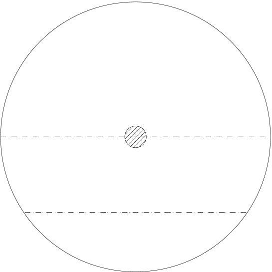
FIG. 2.: A Coleman-De Luccia bounce solution for the case where the flat space bounce radius is much less than $H_{\rm f}^{-1}$. The picture should be visualized as a four-sphere viewed head-on, with $\xi=0$ being the point at the center of the cross-hatched region where the field is on the true vacuum side of the potential barrier; $\xi=\xi_{\rm max}$ is the antipodal point on the opposite side of the sphere. The dashed line passing through $\xi=0$ (and also through $\xi=\xi_{\rm max}$) denotes a three-sphere corresponding to the spatial hypersurface on which the bubble materializes. The three-sphere denoted by the lower dashed line is roughly analogous to the false vacuum initial-state hypersurface in the flat space problem.

There is, however, one difference, related to the point $\xi=\xi_{\rm max}$, that should be pointed out here. One might have expected this to be analogous to $s=\infty$ in the flat space bounce. In the latter, $s=\infty$ defines a three-sphere and corresponds both to spatial infinity on the hypersurface where the bubble materializes and to the initial state hypersurface. By contrast, $\xi=\xi_{\rm max}$ is a single point that lies on the spacelike hypersurface that gives initial data for the Lorentzian problem. However, as can be seen from Fig. 2, it does not lie on the initial state hypersurface.

The deviations from the flat space case become quite significant when the flat space bounce radius is comparable to or greater than $H_{f}^{-1}$. In some such cases, there is no Coleman-De Luccia bounce at all. When there is a bounce, its true vacuum region (whose size may be very different than in the flat space case) occupies a significant fraction of the Euclidean four-sphere, and one can no longer identify even an approximate initial-state hypersurface. Indeed, the asymmetry between the true vacuum interior and the false vacuum exterior is lost to a large degree. This suggests that the two regions can be viewed as being on equal footings, and that the bounce can describe either the production of a true vacuum bubble in a false vacuum background or that of a false vacuum bubble in a true vacuum background, with the initial state determined not by the properties of the bounce solution, but by whether $S_{E}(\phi_{\rm fv})$ or $S_{E}(\phi_{\rm tv})$ is subtracted when calculating $B$. (A detailed examination of this possibility shows that the rates for nucleation of false vacuum bubbles in true vacuum and true vacuum bubbles in false vacuum are related by a factor that has a natural thermal interpretation, and that takes a simple Boltzmann form in some limits [4].)

Finally, note that any multibounce solutions are clearly limited and quite constrained in this large-bounce regime, so there is no exponentiation of the bounce factor; this fact by itself gives a hint of the difficulties of generalizing the path integral calculation of $\Gamma$.

Whether or not there is a Coleman-De Luccia bounce solution, there is always a second type of solution, first pointed out by Hawking and Moss [5], that has no analogue in flat spacetime. Like the pure false vacuum solution, this is homogeneous, but with the scalar field everywhere equal to $\phi_{\rm top}$, its value at the top of the barrier. Calculations exactly analogous to those leading to Eqs. (30)-(32) give

$$\rho(\xi)=H_{\rm top}^{-1}\sin(H_{\rm top}\xi)$$ (33)

and

$$B_{\rm HM}=S_{E}(\phi_{\rm top})-S_{E}(\phi_{\rm fv})={3\over 8}\,\left[-{M_{\rm Pl}^{4}\over V(\phi_{\rm top})}+{M_{\rm Pl}^{4}\over V(\phi_{\rm fv})}\right]\,.$$ (34)

with $H_{\rm top}$ defined by a formula analogous to Eq. (31).

IV new solutions

Our focus in this paper is on a third class of Euclidean solutions that are neither simple bounces nor Hawking-Moss. We continue to assume O(4) symmetry, so Eqs. (25)-(29) still apply. However, we now allow $\phi$ to cross the barrier an arbitrary number of times between $\xi=0$ and $\xi_{\rm max}$; we will denote this number by $k$, so that $k=1$ corresponds to the Coleman-De Luccia bounce. The possibility of multiple barrier crossings is in contrast with the flat space case, where only $k=1$ solutions can exist.

To simplify matters, we will restrict ourselves to the case of a potential with only two local minima. Without any loss of generality we can assume that $\phi_{\rm fv}<\phi_{\rm top}<\phi_{\rm tv}$.

Our problem can be viewed as that of finding values of $\phi_{0}$ for which the initial conditions $\phi(0)=\phi_{0}$, $\dot{\phi}(0)=\rho(0)=0$ imply that $\dot{\phi}(\xi_{\rm max})=0$. By scanning the range $\phi_{\rm fv}<\phi<\phi_{\rm tv}$ for such critical values, all bounce solutions can be found. In fact, because the problem is invariant under the transformation $\xi\rightarrow\xi_{\rm max}-\xi$, every solution with odd $k$ will be encountered twice in such a scan, once as a “false-to-true” bounce and once as a “true-to-false” one. There may also be false-to-false and true-to-true solutions for which the initial and final values of $\phi$ are on the same side of the barrier. These appear either once or twice during the scan, depending on whether or not the two endpoints are identical; we have found examples of both types of behavior.

It should be stressed that our use here of phrases such as “false-to-true” refers only to the variation of $\phi$ as $\xi$ ranges from 0 to $\xi_{\rm max}$. As was pointed out in the previous section, the value of the field at $\xi_{\rm max}$ [in contrast to $\phi(\infty)$ in the flat space bounce] is not necessarily related to the initial state.

In the flat space problem, the possible values of $\phi_{0}$ can be divided into undershoot and overshoot regions, with the critical bounce value lying at the boundary between the regions. In the curved space case, where trajectories can cross $\phi_{\rm top}$ more than once, this overshoot/undershoot classification becomes somewhat ambiguous. Instead, we find it more useful to define a function $h(\phi_{0})$ whose zeroes correspond to the critical trajectories.

An obvious candidate for this function would be the value of $\dot{\phi}(\xi_{\rm max})$ on the trajectory specified by $\phi_{0}$. However, this diverges whenever it is nonzero, and so does not give a satisfactory $h(\phi_{0})$. The quantity $\rho^{3}\dot{\phi}$ is better behaved, but it too can diverge if the trajectory goes into a region where $dV/d\phi$ is unbounded. However, we can avoid any such divergence by modifying the growth of $V$ at large $\phi$. This will have no effect on the critical trajectories, since these remain within the finite interval $\phi_{\rm fv}<\phi<\phi_{\rm tv}$.

Let us therefore define $h(\phi_{0})$ to be the value of $\rho^{3}\dot{\phi}$ at $\xi_{\rm max}$, evaluated on the trajectories of the modified potential. The zeros of $h$ are the values of $\phi_{0}$ that give bounce solutions satisfying the boundary conditions. Although $h$ depends in detail upon precisely how the potential was modified, the locations and nature of its zeros do not, and it is really only these with which we are concerned. There will always be zeros at $\phi_{\rm fv}$, $\phi_{\rm tv}$, and $\phi_{\rm top}$, corresponding to the pure false vacuum, pure true vacuum, and Hawking-Moss solutions, respectively. Depending on the potential these may be the only zeros of $h$, or there may be others.

The plot of $h(\phi_{0})$ evolves as the parameters of the theory are varied. During the course of this evolution the locations of the zeros will vary continuously. The function may also gain or lose zeros, but always in pairs. This can happen either at $\phi_{\rm top}$ or at a point where $h(\phi_{0})$ momentarily develops a double zero. Following the motion, appearance, and disappearance of these zeros provides a framework for the study of the new bounce solutions.

We will start our investigation by considering “small amplitude” solutions in which $\phi$ is confined to the region near $\phi_{\rm top}$, where a linear approximation to Eq. (27) can be applied. We will then follow the evolution of these solutions as a change of parameters takes them outside the linear regime. For some potentials, all bounce solutions arise in this manner. Other potentials admit a second type of solution, that are never confined to the linear region. These can coexist with the former type of solution, or they may be the only type of bounce present.

We begin by introducing an approximation that considerably simplifies the analysis of the bounce equations.

A The fixed background approximation

For the most part, we will focus on the case where the fractional variation of $V(\phi)$ is small as $\phi$ varies over the range from $\phi_{\rm fv}$ to $\phi_{\rm tv}$. This allows us to write

$$V(\phi)=V_{0}+\tilde{V}(\phi)$$ (35)

with $|\tilde{V}(\phi)|\ll V_{0}$ for all relevant values of $\phi$. To leading approximation, the curvature of the Euclidean space is then independent of the value of $\phi$, and we can write

$$\rho(\xi)\approx H^{-1}\sin(H\xi)\equiv\rho_{0}(\xi)$$ (36)

with

$$H^{2}\equiv{8\pi V_{0}\over 3M_{Pl}^{2}}\,.$$ (37)

If we define $y\equiv H\xi$, the equation for $\phi$ becomes, to leading approximation,

$${d^{2}\phi\over dy^{2}}+3\cot y\,{d\phi\over dy}={1\over H^{2}}{d\tilde{V}\over d\phi}$$ (38)

with the boundary conditions that $d\phi/dy$ vanish at both $y=0$ and $y=\pi$.

Once a solution to Eq. (38) has been found, the first correction to the metric can be obtained by substituting this solution into a linearized version of Eq. (28) and solving for $\delta\rho=\rho-\rho_{0}$. Because $\rho_{0}$ is a solution of the zeroth order problem, the terms linear in $\delta\rho$ do not contribute to the action. The terms quadratic in $\delta\rho$ are suppressed relative to the matter terms in the action by a factor of order $\tilde{V}/V_{0}$, allowing us to write

$$S_{E}=-{3\over 8}\,{M_{Pl}^{4}\over V_{0}}+2\pi^{2}\int d\xi\rho_{0}^{3}\left({1\over 2}\dot{\phi}^{2}+\tilde{V}\right)+\cdots\,.$$ (39)

When the false vacuum action is subtracted from that of the bounce, the first terms on the right hand sides cancel, leading to

$$B={9\over 32}{M_{Pl}^{4}\over V_{0}^{2}}\int dy\sin^{3}y\left[{H^{2}\over 2}\left({d\phi\over dy}\right)^{2}+V(\phi)-V(\phi_{\rm fv})\right]\,.$$ (40)

In particular, for the Hawking-Moss solution

$$B_{\rm HM}={3\over 8}\,{M_{Pl}^{4}\over V_{0}^{2}}\left[V(\phi_{\rm top})-V(\phi_{\rm fv})\right]\,.$$ (41)

B Linearized equations

We begin our analysis by seeking small amplitude solutions where $\phi_{0}$ is near $\phi_{\rm top}$ and $\phi$ remains everywhere close to the top of the barrier. These are essentially small perturbations about the Hawking-Moss solution.

We expand the scalar field potential as

$$\tilde{V}(\phi)=V(\phi_{\rm top})+H^{2}\left[-{\beta\over 2}(\phi-\phi_{\rm top})^{2}+{b\over 3}(\phi-\phi_{\rm top})^{3}+{\lambda\over 4}(\phi-\phi_{\rm top})^{4}+\cdots\right]\,.$$ (42)

Because $\phi_{\rm top}$ is a maximum of the potential, $\beta$ is necessarily positive, and

$$\beta={|V^{\prime\prime}(\phi_{\rm top})|\over H^{2}}\,.$$ (43)

The sign of $b$ can be reversed by a simple redefinition of $\phi$, and hence is not physically significant. Finally, $\lambda$ can take either sign, although it must be positive if there are no higher order terms in the potential.

If the field remains sufficiently close to $\phi_{\rm top}$, the cubic and higher terms in the potential can be dropped in a first approximation, so that Eq. (38) takes the form

$$0={d^{2}\phi\over dy^{2}}+3\cot y\,{d\phi\over dy}+\beta(\phi-\phi_{\rm top})\,.$$ (44)

If we write $\phi(y)-\phi_{\rm top}=f(y)\sin^{-3/2}y$, this becomes

$$0={d^{2}f\over dy^{2}}+\left(\beta+{3\over 2}-{3\over 4}\cot^{2}y\right)f\,.$$ (45)

Except near the outer edges of the interval $0\leq y\leq\pi$, the last term in the brackets can be ignored, and we find that

$$\phi(y)-\phi_{\rm top}\approx A{\sin(\sqrt{\beta+3/2}\,y+\delta)\over\sin^{3/2}y}\,,$$ (46)

with $A$ and $\delta$ constants.

More precisely, we can note that an exact solution of Eq. (44) is given by a Gegenbauer, or ultraspherical, function

$$\phi(y)-\phi_{\rm top}=AC_{\alpha}^{3/2}(\cos y)$$ (47)

with $\alpha$ the positive root of

$$\alpha(\alpha+3)=\beta\,.$$ (48)

The fact that $C_{\alpha}^{3/2}(1)$ is finite for all real positive $\alpha$ guarantees the vanishing of $d\phi/dy$ at $y=0$; it is this condition that eliminates the Gegenbauer function of the second kind, $D_{\alpha}^{3/2}(\cos y)$. The second boundary condition, that $d\phi/dy$ also vanish at $y=\pi$, is only satisfied if $\alpha$ is an integer. Hence, the linearized approximation, Eq. (44), has an acceptable solution only if $V^{\prime\prime}(\phi_{\rm top})=N(N+3)H^{2}$ for $N=1,2,\dots$. Because $C_{N}^{3/2}(\cos y)$ has $N$ zeros in the range $0\leq y\leq\pi$, these solutions are bounces with with $k=N$ crossings of the barrier.

We recall, for later use, that the Gegenbauer functions for integer $N$ are polynomials. If defined with the standard normalization

$$C_{N}^{3/2}(1)={(N+1)(N+2)\over 2}\,,$$ (49)

they obey the orthogonality relation

$$\int_{-1}^{1}\,dx\,(1-x^{2})C_{M}^{3/2}(x)C_{N}^{3/2}(x)=\delta_{M,N}\,{2(N+1)(N+2)\over(2N+3)}\equiv\delta_{M,N}\,k_{N}\,.$$ (50)

C Incorporating nonlinearities

The linearized equations only have solutions obeying the boundary conditions when $\beta$ is equal to one of a discrete set of critical values. This condition is relaxed once the nonlinear terms are included. This is quite similar to the way in which adding anharmonic terms to a simple harmonic oscillator allows small amplitude oscillations with a continuous range of periods. Just as the amplitude is related to the period in the oscillator problem, the amplitude of the bounce solutions is determined by the distance $\Delta=\beta-N(N+3)$ from the critical value.

Because the Gegenbauer polynomials form a complete set, an arbitrary function $\phi(y)$ obeying the boundary conditions of Eq. (29) can be expanded as

$$\phi(y)=\phi_{\rm top}+{1\over\sqrt{|\lambda|}}\sum_{M=0}^{\infty}A_{M}C_{M}^{3/2}(y)\,,$$ (51)

where the coefficients $A_{M}$ are dimensionless. Substituting this into Eq. (38) and retaining the contributions from the cubic and quartic terms in the expansion of the potential yields

$$0=\sum_{M=0}^{\infty}C_{M}^{3/2}(y)\left\{[\beta-M(M+3)]A_{M}-{b\over\sqrt{|\lambda|}}\sum_{I,J}A_{I}A_{J}p_{IJ;M}-{\rm sgn}\,(\lambda)\sum_{I,J,K}A_{I}A_{J}A_{K}q_{IJK;M}\right\}$$ (52)

where the terms involving

$$p_{IJ;M}=k_{M}^{-1/2}\int_{-1}^{1}dy\,C_{I}^{3/2}(y)C_{J}^{3/2}(y)C_{M}^{3/2}(y)$$ (53)

and

$$q_{IJK;M}=k_{M}^{-1/2}\int_{-1}^{1}dy\,C_{I}^{3/2}(y)C_{J}^{3/2}(y)C_{K}^{3/2}(y)C_{M}^{3/2}(y)$$ (54)

arise from the expansion of the $\phi^{2}$ and $\phi^{3}$ terms, and the normalization factor $k_{M}$ is defined by Eq. (50). Note that $p_{IJ;M}$ vanishes if the sum of any two indices is greater than the third, and that $q_{NNN;N}>0$ for all $N$.

Each term of the sum in Eq. (52) must vanish separately. For $|\Delta|$ sufficiently small, we expect to find a small amplitude solution in which a single coefficient, $A_{N}$, is dominant. Explicitly,

$$0=\Delta A_{N}-{b\over\sqrt{|\lambda|}}p_{NN;N}A_{N}^{2}-{2b\over\sqrt{|\lambda|}}\sum_{M\neq N}p_{MN;N}A_{M}A_{N}-{\rm sgn}\,(\lambda)q_{NNN;N}A_{N}^{3}+\cdots$$ (55)

and

$$0=[\beta-M(M+3)]A_{M}-{b\over\sqrt{|\lambda|}}\,p_{NN;M}A_{N}^{2}+\cdots\,,\qquad M\neq N\,,$$ (56)

where in each equation the omitted terms are higher order in $A_{N}$. Using the second equation to eliminate $A_{M}$ from the first leads to

$$0=\Delta-{b\over\sqrt{|\lambda|}}p_{NN;N}A_{N}-cA_{N}^{2}+O(A_{N}^{3})\,,$$ (57)

where

$$c={\rm sgn}\,(\lambda)q_{NNN;N}+{2b^{2}\over|\lambda|}\sum_{M\neq N}^{2N}\left[{1\over\beta-M(M+3)}\right]p_{NN;M}p_{NM;N}\,.$$ (58)

This gives

$$A_{N}={1\over 2c}\left[-{bp_{NN;N}\over\sqrt{|\lambda|}}\pm\sqrt{{b^{2}(p_{NN;N})^{2}\over|\lambda|}+4c\Delta}\right]\,.$$ (59)

If the cubic term in Eq. (42) vanishes, $b=0$, there are real solutions for $A_{N}$ only if $c\Delta>0$, with $A_{N}=\pm\sqrt{\Delta/c}$. Thus, for $\lambda>0$ there are no small amplitude bounces if $\beta<N(N+3)$. As $\beta$ is increased past this critical value, two solutions appear. For odd $N$ these are a physically equivalent true-to-false and false-to-true pair, while for even $N$ they are two distinct solutions, one true-to-true and the other false-to-false. Things are similar if $\lambda<0$, except that the solutions only exist for $\beta<N(N+3)$.

For nonzero $b$ and odd $N$, the situation is almost the same. Because $p_{NN;N}$ vanishes for odd $N$, the condition for existence of a solution is again that $c\Delta>0$, although now $c$ and $\lambda$ may have different signs. As before, there are two distinct but physically equivalent small amplitude solutions, and these appear at the critical value $\beta=N(N+3)$.

For nonzero $b$ and even $N$, the situation is more complicated. From Eq. (59), we see that the critical value of $\beta$ where solutions first appear is not $\beta=N(N+3)$, but rather

$$\beta=N(N+3)-{b^{2}\over 4c|\lambda|}(p_{NN;N})^{2}\,,$$ (60)

which is a bit smaller (larger) if $c$ is positive (negative). In contrast with the previous cases, when the solutions first appear they have a finite amplitude and both have the same sign for $A_{N}$. As $\beta$ is increased (decreased) through $N(N+3)$, one of the solutions passes through zero and then takes on the opposite sign. After this point the two solutions remain of opposite sign, with the magnitude of $A_{N}$ increasing for both.

Some words of caution are in order here. Our analysis is valid only for sufficiently small $A_{N}$. If $b/\sqrt{|\lambda|}$ is too large, this condition may not be met when $\beta$ is given by Eq. (60), in which case it will never be satisfied by the larger of the two solutions. However, as $\Delta\rightarrow 0$, the other solution for $A_{N}$ tends to zero, and so should be reliable. As discussed at the beginning of this section, the zeros of $h(\phi_{0})$ appear or disappear in pairs. Hence, the existence of one small amplitude solution implies the existence of the second. We therefore expect the qualitative features — the emergence of two solutions, with finite amplitude, at a value of $\beta$ not corresponding to an integer — to be valid even if the quantitative analysis is not completely reliable.

The results of this section can be compared with the analysis of Jensen and Steinhardt[14]. They argued that if $|V^{\prime\prime}|$ is monotonically decreasing as one moves from the top of the potential toward the false vacuum there will be a unique $k=1$ Coleman-De Luccia bounce if (in our language) $\beta>4$, and that this solution merges with the Hawking-Moss solution as $\beta\rightarrow 4$. When applied to Eq. (42), their condition on $V^{\prime\prime}$ translates into the statement that $\lambda>0$. If $b^{2}/\lambda$ is not too large, $c$ will also be positive, and our results will agree with theirs. However, for $b^{2}/\lambda$ sufficiently large, $c$ can be negative even though $\lambda$ is not. In this case, $\beta=4$ is an upper bound for the existence of these solutions, and our results will disagree with their analysis. We believe that this can be attributed to the fact that their claims are based on the argument that the potential gets “flatter” as one moves away from the top of the barrier; for large $b$ this is true, in the relevant range, only on one side of the potential.

Perturbative methods similar to those used in this section have recently been applied to the calculation of the bounce action [15].

V Numerical results for $\lambda>0$

Once the amplitude become large, the analysis based on a single dominant term in Eq. (51) fails, and we must resort to numerical methods. Before describing our numerical results, we outline some qualitative arguments that may provide some useful insight. We focus here on the case $\lambda>0$, where the quartic term in the potential is positive. We will return to the $\lambda<0$ case in Sec. VI.

We have seen that $h(\phi_{0})$ has a zero at $\phi_{\rm top}$, corresponding to the Hawking-Moss solution, for all values of $\beta$. As $\beta$ increases, pairs of new zeros, corresponding to bounce solutions with ever increasing values of $k$, appear at $\phi_{\rm top}$ as $\beta$ passes through successive critical values. When the analysis of Sec. IV C can be applied, these zeros move apart as $\beta$ increases. We expect this behavior to continue even after the zeros have moved beyond the small amplitude regime. Thus, at any given $\beta$ there should be a sequence of bounce solutions. For $b=0$ and $N(N+3)<\beta<(N+1)(N+4)$, there would be two solutions each for $k=1,2,\dots,N$, with the two solutions for each odd $k$ simply being “$y$-reversed” versions of each other. For nonzero $b$ the picture would be similar, except that the new solutions for even $N$ appear somewhat before $\beta=N(N+3)$. Figure 3 gives a schematic illustration of the expected pattern of zeros.

FIG. 3.: A schematic plot of the starting points of bounce solutions to a $\lambda>0$ theory, such as that discussed in Sec. V, with $\beta$ slightly greater than 28. The numbers next to the points represent the number of times the solution crosses the top of the potential barrier.

We can also make some predictions about the form of these solutions. It seems reasonable to expect that, even after $\phi_{0}$ has moved well beyond the small amplitude regime, the average period of the oscillations will continue to be determined to leading order by $\beta$. Increasing $\beta$ will decrease this period, and so should cause a plot of the oscillations of $\phi$ to shrink horizontally at the same time that it is expanding vertically. With the number of oscillations in a given solution remaining fixed, this will open up “gaps” at the ends of the interval. In order to satisfy the boundary conditions that $d\phi/dy=0$ at $y=0$ and $y=\pi$, the field must be relatively constant in these gaps. This, in turn, implies that the field near the end points must be close to one or the other of the minima of the potential. As $\beta$ is increased further, the fraction of the $y$-interval occupied by oscillations will continue to decrease, while the regions occupied by these false and true vacuum regions will expand.

We have tested these ideas numerically by considering a theory governed by a quartic potential than can be written in the form

$$V=\beta H^{2}v^{2}\left[-{1\over 2}\psi^{2}-{g\over 3}\psi^{3}+{1\over 4}\psi^{4}\right]+V_{0}\,,$$ (61)

where $\psi=\phi/v$ is a dimensionless field that has been rescaled so that for $g=0$ the minima of the potential are at $\psi=\pm 1$; in the notation of Eq. (42), this corresponds to $b=-g\beta/2v$ and $\lambda=\beta/v^{2}$. We focus here on our results for a single value of $\beta$. However, we have explored solutions for a much wider range of values, going as high as $10^{4}$. In all cases, our results are consistent with the picture we describe here.

In Fig. 4 we show the bounce solutions for $g=1/2\sqrt{2}$ and $\beta=70.03$, corresponding to $N=7$. As expected, we find solutions for every integral value of $k$ up to $k=7$, with two distinct solutions for each even value of $k$. Although it is barely apparent on the figures (except for $k=7$), it should be noted that, among solutions starting on a given side of the barrier, the initial value $\phi_{0}$ monotonically approaches $\phi_{\rm top}$ as $k$ increases, in accord with our expectations.

FIG. 4.: Bounce solutions for the asymmetric ($g={1\over 2\sqrt{2}}$) potential discussed in the text. For these solutions $\beta=70.03$.

The $k=1$ solution is the Coleman-De Luccia bounce. For $k=2$, there are two solutions. One starts and ends near the true vacuum, and might be viewed as a two-bounce solution analogous to the flat space multibounce solutions that are encountered in the path integral treatment. Indeed, its field profile is very close to that expected from two independent bounces and its action is approximately twice that of the single bounce. The other $k=2$ solution starts and ends near the false vacuum. It, too, might be interpreted as a two-bounce solution, if one took the Coleman-De Luccia bounce to represent decay from the true vacuum to the false. From this viewpoint, the false vacuum region corresponds to the bubble interior; since this is large compared to the size of the four-sphere, there must be significant distortion to be able to fit in two bounces. Note that even in the region separating the two “interiors” $\phi$ does not get very close to its true vacuum value.

The solutions with $k>2$ all have intermediate oscillations about $\phi_{\rm top}$. As expected, the frequency of these oscillations seems to be determined primarily by $\beta$, with the separation between zeros of the field being roughly independent of $k$. The existence of intermediate oscillations seems to have little effect on the true vacuum bubble region, with the field profiles near $y=\pi$ for the $k<7$ false-to-true solutions and near $y=0$ and $y=\pi$ for all the true-to-true solutions being very similar to that for the corresponding region of the Coleman-De Luccia solution. This is not so for the false vacuum regions.

The plot for the $k=7$ solution shows that the linear approximation works quite well, as should be expected with $\beta$ so close to the critical value of 70. The numerical solution is indistinguishable to the eye from the Gegenbauer polynomial, and the initial value, $\phi_{0}$, agrees well with the prediction of Eq. (59).

In Fig. 5, we show the analogous results for the case of $g=0$, where the two minima are degenerate. In flat spacetime, there would be no bounces for this case but, as we see, this is no longer so when gravitational effects are included.

FIG. 5.: Bounce solutions for the symmetric ($g=0$) potential with two degenerate vacua that is discussed in the text. Again, $\beta=70.03$.

Finally, in Figs. 6 and 7 we show the actions for these solutions. (More precisely, what we actually plot in these figures is $B=S_{\rm bounce}-S_{\rm fv}$, which is the quantity that would appear in the exponent if these solutions were interpreted as contributions to the process of tunneling out of the false vacuum.) As $k$ increases, $B$ approaches the Hawking-Moss value $B_{\rm HM}$. This can be understood by noting that in the linearized approximation the contribution from the gradient terms exactly cancels that from the oscillatory part of the potential term, so that the total action is exactly equal to that of the Hawking-Moss solution.

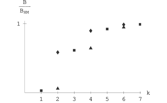
FIG. 6.: The tunneling exponent $B=S(\phi_{\rm bounce})-S(\phi_{\rm fv})$ for the asymmetric potential bounce solutions shown in Fig. 4. The values are given as fractions of the Hawking-Moss value, and are plotted as a function of the number of times the solution crosses the top of the barrier. Boxes correspond to solutions which interpolate between the true and false vacuum sides of the barrier, diamonds correspond to “true-to-true” solutions, and triangles to “false-to-false” ones.

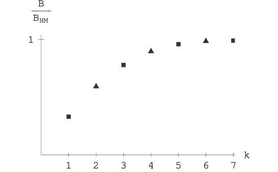
FIG. 7.: The tunneling exponent $B$ for the symmetric potential bounce solutions shown in Fig. 5. The values are given as fractions of the Hawking-Moss value, and are plotted as a function of the number of times the solution crosses the top of the barrier. Boxes correspond to solutions which interpolate between the the two vacua, and triangles correspond to solutions which begin and end on the same side of the barrier.

VI Bounces with flat potential barriers

Our analysis of small amplitude bounces in the previous two sections showed that for a wide class of potentials — those with a positive fourth derivative, and not too large a third derivative, at $\phi_{\rm top}$ — there is neither a small oscillation bounce nor a bounce smoothly related to a small oscillation bounce if $|V^{\prime\prime}(\phi_{\rm top})|<4H^{2}$. This result is intuitively quite plausible. One might expect $|V^{\prime\prime}(\phi_{\rm top})|^{-1/2}$ to set a natural scale for the size of the bounce, so that if this were too large, relative to the radius $H^{-1}$, the bounce would not fit on the four-sphere.

However, our results for the case where the fourth derivative (or more precisely, the related quantity $c$) is negative show that this seemingly plausible argument cannot be quite correct. For this case we saw that there was a small amplitude $k=1$ bounce only for a range of values extending downward from $\beta=4$. One logical possibility is that these solutions continue (although not necessarily with small amplitudes) all the way down to $\beta=0$. Alternatively, there might be some minimum value $\beta_{\rm min}$ (which could depend on the other parameters of the theory) for which the bounce exists. Since solutions can only appear and disappear in pairs, this latter possibility would require the existence of a second solution, which would also appear at $\beta_{\rm min}$ but which would persist beyond $\beta=4$.

In this section we will explore this direction in more detail. Because the potentials that evade the $\beta>4$ bound are characterized by being relatively flat at the top of the barrier, we begin by studying a toy model, defined by the potential

$$V=\cases{C(\phi+a)+V_{0}\,,\qquad\phi<-a\cr\cr V_{0}\,,\qquad-a\leq\phi\leq a\cr\cr-C(\phi-a)+V_{0}\,,\qquad\phi>a}$$ (62)

that is absolutely flat at the top. This potential has the additional advantage that the field equation can be solved analytically.

Inserting this potential into Eq. (38), and defining

$$\chi(y)=\sin^{3}y{d\phi\over dy}\,,$$ (63)

leads to

$${d\chi\over dy}=\cases{a\gamma\sin^{3}y\,,\qquad\phi<-a\cr\cr 0\,,\qquad-a\leq\phi\leq a\cr\cr-a\gamma\sin^{3}y\,,\qquad\phi>a}$$ (64)

where

$$\gamma={C\over aH^{2}}\,.$$ (65)

Because $C/a$ gives a rough measure of the average value of $|V^{\prime\prime}|$ for our toy potential, $\gamma$ is somewhat analogous to the quantity $\beta$ that appeared in the analysis of the two previous sections.

We first seek a $k=1$ (Coleman-De Luccia) bounce. The symmetry of the potential implies that this solution (as well as any other bounce with odd $k$) must have $\phi(\pi/2)=0$. Let $\phi(0)=\phi_{0}<-a$, and define $y_{1}<\pi/2$ by the condition $\phi(y_{1})=-a$. Integrating Eq. (64) over the interval $0\leq y\leq y_{1}$ gives

$$\chi(y_{1})=a\gamma\int_{0}^{y_{1}}du\sin^{3}u\,.$$ (66)

The fact that $\chi$ is constant over the flat part of the potential implies that

$$a=\phi(\pi/2)-\phi(y_{1})=\chi(y_{1})\int_{y_{1}}^{\pi/2}{dv\over\sin^{3}v}\,.$$ (67)

Combining these two equations gives the requirement that

$${1\over\gamma}=\int_{0}^{y_{1}}du\sin^{3}u\int_{y_{1}}^{\pi/2}{dv\over\sin^{3}v}\equiv F_{1}(y_{1})\,.$$ (68)

Once a value of $y_{1}$ satisfying this condition has been found, it is a straightforward matter to find $\phi_{0}$ by integrating back from $y_{1}$ to $y=0$ and to then integrate forward to obtain $\phi(y)$ for all $y$.

From the plot of $F_{1}(y)$ shown in Fig. 8, we see that Eq. (68) has no solutions, and hence there is no Coleman-De Luccia bounce, if $\gamma<1/{\rm Max}\,[F_{1}(y)]\approx 7.70$. For any $\gamma$ greater than this critical value there are two acceptable values for $y_{1}$, and thus two distinct Coleman-De Luccia bounces. As examples of this, in Fig. 9 we show the two bounces solutions for $\gamma=10$.

FIG. 8.: The functions $F_{1}(y_{1})$ and $F_{2}(y_{1})$ for the toy model defined by Eq. (62)

FIG. 9.: The two $k=1$ bounces for our linear toy model when $\gamma=10$.

In general, these values for $y_{1}$ can only be found numerically. However, approximate expressions can be obtained for the limiting case $\gamma\gg 1$. In one solution, with

$$y_{1}\approx\sqrt{8\over\gamma}\qquad\qquad\phi_{0}\approx-a\left(1+{1\over\gamma}\right)\,,$$ (69)

the field is mostly on the flat part of the potential. In the other solution, with

$$y_{1}\approx{\pi\over 2}-{3\over 2\gamma}\qquad\qquad\phi_{0}\approx-\left({1+\ln 4\over 6}\right)a\gamma\approx-.398a\gamma\,,$$ (70)

the field is mostly on the sloping parts of the potential. The latter solution has the lower action.

For $k=2$ (or any even value of $k$), $d\phi/dy$ vanishes at $y=\pi/2$. Let us define $y_{1}<y_{2}<\pi/2$ by $\phi(y_{1})=-\phi(y_{2})=-a$. Integrating Eq. (64) then gives

$$\chi(y_{1})=a\gamma\int_{0}^{y_{1}}du\sin^{3}u$$ (71)

$$\chi(y_{2})=a\gamma\int_{y_{2}}^{\pi/2}du\sin^{3}u\,.$$ (72)

Because the field is in the flat part of the potential for $y_{1}<y<y_{2}$, these integrals must be equal; this implicitly defines $y_{2}$ as a function of $y_{1}$.

By analogy with Eq. (67), we also have

$$2a=\phi(y_{2})-\phi(y_{1})=\chi(y_{1})\int_{y_{1}}^{y_{2}(y_{1})}{du\over\sin^{3}u}\equiv 2a\gamma F_{2}(y_{1})\,.$$ (73)

Referring again to Fig. 8, we see that there are no solutions for $\gamma<1/{\rm Max}\,[F_{2}(y)]\approx 21.7$, but two solutions for all larger values of $\gamma$. In the cases where there are solutions, these have values of $y_{1}$ (and also of $\phi_{0}$) that fall between the corresponding $k=1$ values. In the limit $\gamma\gg 1$, the $k=2$ solutions have

$$y_{1}\approx\sqrt{16\over\gamma}\qquad\qquad\phi_{0}\approx-a\left(1+{2\over\gamma}\right)$$ (74)

and

$$y_{1}\approx 1.22\qquad\qquad\phi_{0}\approx-.319a\gamma\,.$$ (75)

This procedure can be extended to all higher values of $k$. For any given $k$, solutions only exist if $\gamma$ is larger than a critical value $\gamma_{\rm cr}(k)$; if $\gamma>\gamma_{\rm cr}(k)$ there are two allowed values for $\phi_{0}$, both of which fall between the allowed valued for the $k-1$ solutions with the same $\gamma$. For $k=3$, the critical value is 42.7. More generally, $\gamma_{\rm cr}(k)$ is an increasing function of $k$ and is $O(k^{2})$ for large $k$; this behavior is reminiscent of the critical values of $\beta$ that govern the appearance of small amplitude solutions in potentials with a positive quartic term.

The situation is illustrated in Fig. 10, which gives a schematic summary of the possible values for $\phi_{0}$ for a given value of $\gamma$. As $\gamma$ is increased, the zeros marked by closed circles move outward, while those marked by open circles move inward. When $\gamma$ reaches a critical value, two new pairs of coincident zeros (one pair on each side of the potential) appear and then begin to separate. With increasing $\gamma$, accumulations of open circles develop near $\phi=\pm a$, while the outwardly moving closed circles become further and further apart.

FIG. 10.: A schematic graph of the starting points of bounce solutions to our linear toy model. Closed circles represent solutions which move outward as $H$ is decreased, and open circles represent solutions which move inward. The numbers next to the points represent the number of times the solution crosses the top of the potential barrier.

The actions of these solutions may be either greater or less than that of the Hawking-Moss solution. For example, the $k=1$ solution with the smaller $|\phi_{0}|$ always has a higher action than both the other $k=1$ solution and the Hawking-Moss. The action of the other $k=1$ solution is greater than $S_{\rm HM}$ for small $\gamma$, but not for large $\gamma$.

This toy model has the advantages of allowing analytic solution and of emphasizing that it is possible to have a Coleman-De Luccia bounce with an arbitrarily small value of $|V^{\prime\prime}(\phi_{\rm top})|$. However, one consequence of its somewhat artificial form is that the bounce solutions have some special properties that we would not expect in a more generic potential. For example, the values of $\phi_{0}$ that move inward with increasing $\gamma$ (i.e., those indicated by open circles in Fig. 10) accumulate near the “corners” of the potential at $\pm a$, but never move further inward where they might meet and “annihilate”.

A less artificial example can be obtained by considering a potential of the form $V=-a\phi^{2}-b\phi^{4}+c\phi^{6}$, with $a$, $b$, and $c$ all positive. With three parameters to vary, it is possible to make the potential relatively flat, as defined by a scale-independent criterion, at the top of the barrier. For example, if $\pm v$ are the minima of the potential, we can define an averaged second derivative $V^{\prime\prime}_{\rm avg}$ by

$$V^{\prime\prime}_{\rm avg}={V^{\prime}(v/2)-V^{\prime}(-v/2)\over v}\,.$$ (76)

By choosing $b^{2}\gg ac$ we can make $|V^{\prime\prime}(0)|\ll|V^{\prime\prime}_{\rm avg}|$.

We have followed the evolution of the bounce solutions for such a potential (with $b^{2}/ac=80$) as $H$ is varied with the parameters in the potential held fixed. For very large $H$, there are no bounce solutions, in analogy with the low $\beta$ or low $\gamma$ behavior of our previous examples. As $H$ is decreased, two pairs of zeros, corresponding to initial values for $k=1$ bounces, appear at nonzero points on opposite sides of the barrier, just as in our toy model. (In the example we studied, these first appeared at $|V^{\prime\prime}_{\rm avg}|/H^{2}=4.03$.) As $H$ is reduced further, each pair splits, with one zero moving inward and one outward. With further decreases in $H$, additional zeros, corresponding to bounces with $k=2$, $k=3$, etc. appear, just as in the toy model.

In contrast with the toy model, the inwardly moving zeros proceed all the way in to $\phi=0$, reaching that point exactly when predicted by the analysis of Sec. IV C. Thus, two $k=1$ zeros meet and annihilate when $H^{2}=a/2$, two $k=2$ zeros annihilate when $H^{2}=a/5$, etc. We have also encountered a more complex type of behavior for some values of the parameters. As described above, two pairs of $k=2$ zeros appear at a certain critical value of $H$. After moving inward some distance, each of the inner zeros splits into three zeros. These then separate for a time, and then rejoin to form a single zero, which eventually moves to $\phi=0$. A schematic snapshot of this example for a fixed value of $H$ is shown in Fig. 11.

FIG. 11.: A schematic graph of the starting points of bounce solutions for the sixth-order potential discussed in the text. Closed circles represent solutions which move towards one of the vacua as $H$ is decreased, and open circles represent solutions which move towards the top. The numbers next to the points represent the number of times the solution crosses the top of the potential barrier.

The examples considered in this section clearly demonstrate that the existence of a Coleman-De Luccia bounce need not impose a lower bound on $|V^{\prime\prime}(\phi_{\rm top})|$. However, they suggest that a more generalized version of this bound, involving an averaged value of $|V^{\prime\prime}|/H^{2}$, does hold. This is consistent with the results of [17], where it is argued that a necessary condition for the existence of a Coleman-De Luccia bounce is that $|V^{\prime\prime}(\phi)|/H^{2}>4$ for some value of $\phi$.

VII Concluding remarks

In this concluding section we will first summarize our results and then discuss how they might be affected if we relax some of the restrictions that we have imposed to simplify the analysis. We will then briefly discuss the physical implications and interpretation of these solutions.

A Summary

In this paper we have studied in some detail a class of oscillating bounce solutions that arise when the effects of gravity on vacuum tunneling processes are taken into account. These are qualitatively distinct from the Coleman-De Luccia and Hawking-Moss solutions. In fact, they can be viewed as, in a sense, interpolating between these two limiting cases.

These oscillating bounces exist on a space that is topologically a Euclidean four-sphere. They are O(4)-symmetric, so that the scalar field depends only on the parameter $\xi$, which is proportional to the azimuthal angle. At $k\geq 1$ values of $\xi$ the scalar field takes on its value at the top of the potential barrier. These values correspond to $k$ three-spheres that can be viewed as dividing the four-sphere into two end caps and $k-1$ bands. Typically, in each of the end cap regions the field approaches close to, but does not quite reach, one of the two possible vacuum values. In the intermediate band regions the field is alternately on the true or false vacuum side of the barrier, although it does not generally wander very far from the top of the barrier, with this deviation decreasing as $k$ increases.

For $k=1$, the solution is simply the Coleman-De Luccia bounce. The $k=2$ solution for which the field in both end caps is in the true vacuum region can be viewed as a two-bounce solution. However, the solutions with higher values of $k$ are not in any sense multi-bounce solutions. For any fixed value of the parameters of the theory, there are only a finite number (possibly zero) of these solutions. When solutions exist, they have values of $k$ taking on all integer values from 1 to some $k_{\rm max}$, with possibly several distinct solutions for the same value of $k$. The determination of precisely how many solutions exist is closely related to the older problem of determining when a potential admits a Coleman-De Luccia bounce.

In a rough sense, the controlling quantity here is the ratio of the second derivative of the potential to the value of $H^{2}$. This is physically plausible, since for “typical” potentials $V^{\prime\prime}$ is related to the characteristic mass scale, which in turn determines the characteristic size of a classical solution. If this last quantity were too large, one might imagine that the bounce would not “fit” on the four-sphere. Early discussions focused on $\beta\equiv|V^{\prime\prime}(\phi_{\rm top})|/H^{2}$, and argued that there was no Coleman-De Luccia bounce if $\beta<4$. We have shown that for a broad class potentials $\beta$ is indeed the controlling parameter and that $k_{\rm max}=N$, where $N$ is the largest integer such that $N(N+3)<\beta$. As $\beta$ is increased through one of these critical values, two (possibly equivalent) $k=N$ solutions appear. Precisely at the critical value, the new solutions are identical to the Hawking-Moss solution, and so can be thought of as being “all wall”. (As described in Sec. IV, matters can be slightly more complicated if $k$ is an even number.)

Not all potentials give this behavior, as is evident from our results for the case where the fourth derivative of the potential is negative at the top of the barrier. Here, the critical values of $\beta$ give upper, rather than lower, limits for the existence of small amplitude bounce solutions. The situation is somewhat clarified by considering potentials where the barrier is atypically flat. For these, the parameter whose value determines the first appearance of a bounce is not the second derivative at the top of the barrier. Instead, one can use an averaged value of $|V^{\prime\prime}|/H^{2}$ (whose precise definition may vary from case to case) to define a quantity $\gamma$. As $\gamma$ is increased through a $k$-dependent critical value $\gamma_{1}$, a pair of $k$-solutions appears. These coincide, and are nontrivial, when they first appear. In the simplest case, one of these will persist for all $\gamma>\gamma_{1}$, while the other survives only for a finite range $\gamma_{1}<\gamma<\gamma_{2}$, with the parameters that give $\gamma=\gamma_{2}$ also giving $\beta=k(k+3)$. When this critical point is reached, the latter solution and its $\xi$-reversed image annihilate and merge into the Hawking-Moss solution. More complicated patterns are also possible, but must satisfy the constraint that solutions only appear and disappear in pairs. To satisfy this requirement there must be at least one solution that survives for arbitrarily large $\gamma$, and a second solution that either merges with the Hawking-Moss at a finite value of $\gamma$ or, as with our toy model, also persists for arbitrarily large $\gamma$.

B Robustness of our results

To simplify our analysis, we have imposed two restrictions. First, we have only considered solutions with O(4) symmetry. Second, we have assumed that the potential is such that we can use the fixed background approximation. We must now ask how robust our results are, and how they might change were these restrictions relaxed.

The restriction to O(4)-symmetric configurations is the common practice in flat space treatments of vacuum tunneling. For single-field potentials satisfying a rather plausible set of conditions, it can even be shown that the lowest action bounce has O(4) symmetry. Indeed, although there are nonsymmetric approximate stationary points corresponding to several widely separated bounces, it may well be that most theories admit no bounce solutions without O(4) symmetry.

This situation is no longer the case when gravitational corrections are included, largely because the Euclidean space is now a compact manifold. To see this, consider the regime where the true vacuum bubble of the Coleman-De Luccia bounce has a radius much less than $H^{-1}$. Now arrange several such bubbles in a maximally symmetric fashion around the four-sphere (e.g., at the six vertices of a five-dimensional hypertetrahedron). It is clear that some mild local smoothing of the configuration will give a stationary point of the action, and hence a bounce solution without O(4) symmetry. The solution will, however, be invariant under a discrete subgroup of O(5). It is quite possible that there might be additional solutions, with oscillatory behavior, with the same discrete symmetry. However, there no reason to expect more than a finite number of these. Further, we would expect that the actual number of such solutions would have a dependence on the parameters of the theory that is similar to that found for the O(4)-symmetric solutions.

A more significant limitation on our analysis is the use of the fixed background approximation, which is clearly inapplicable to many potentials of interest. Nevertheless, we expect most if not all of the qualitative, and indeed many of the quantitative, features of our results to persist. Thus, for solutions that begin as small deviations from the Hawking-Moss solution when $\beta$ reaches a critical value (either from above or below), the value of $\beta_{\rm cr}$ will be exactly as in our analysis, provided that $H$ is calculated using $V(\phi_{\rm top})$.

A second case to consider is the toy model of Sec. VI. Let us assume that the linear falloff of the potential is terminated at some finite value of $|\phi|$ in such a way that $V(\phi)$ remains everywhere positive. Further, let $\gamma$ still be defined using the value of the potential at the top of the barrier. The fact that $V(\phi)$ is actually lower than this in some regions would have the effect of decreasing the effective value of $H$; from Eq. (28), we see that the nonzero $\dot{\phi}$ acts in the same direction. The Euclidean space will therefore be larger, making it easier to fit in a bounce solution. As a result, we expect a reduction in the values of $\gamma$ at which solutions for a given $k$ will first appear, and thus an even larger range of parameters that allow a bounce with an absolutely flat potential.

C Physical interpretation

We now turn to the physical interpretation of these solutions. As with the Coleman-De Luccia and Hawking-Moss bounces, the hypersurface passing through $\xi=0$ and $\xi=\xi_{\rm max}$ gives the initial data for the classical evolution after the vacuum transition governed by the bounce. This hypersurface is a three-sphere of radius $\sim H^{-1}$, apparently implying that the transition takes place at the “waist” of the de Sitter hyperboloid. This is generally understood to be an artifact of the formalism, with the physical results instead being adapted to a single horizon volume.

Formally, the classical evolution can be obtained by an analytic continuation of the bounce solution. In doing so, particular care must be taken at the points $\xi=0$ and $\xi=\xi_{\rm max}$ of the Euclidean solution. After rotation to a Lorentzian signature these become the lightlike boundaries of two antipodal regions on the de Sitter hyperboloid [13]; this generalizes the manner in which the origin of the flat space Euclidean solution becomes a lightcone after the Wick rotation to Minkowski space.

In the case of the Coleman-De Luccia bounce, this procedure yields a Lorentzian spacetime in which portions of two de Sitter spaces, corresponding to the two vacua, are separated by a well-defined bubble wall. When the initial bubble size is small, the bounce can be viewed as having an initial state hypersurface corresponding to the false vacuum (see Fig. 2), and the vacuum transition is most naturally interpreted as quantum mechanical tunneling. When the initial bubble size is comparable to $H^{-1}$, the initial state is not evident in the bounce, but is instead determined only by which vacuum action is subtracted in the calculation of $B$. The transition thus has a more thermal character, reflecting the existence of a nonzero de Sitter temperature $T_{\rm dS}$.

The Hawking-Moss solution is even more clearly thermal in character. Here the initial data for the classical evolution is a homogeneous region with the field balanced at the top of the potential barrier. Although, strictly speaking, the classical Lorentzian evolution would leave the scalar field at the top of the barrier forever, this solution is unstable against small fluctuations and so will break up, in a stochastic fashion, into regions that evolve toward one or the other of the two vacua.

The oscillating bounces yield a hybrid of these two cases. The end cap regions near $\xi=0$ and $\xi=\xi_{\rm max}$ evolve into two vacuum regions bounded by well-defined walls; these vacua can be the same or different, and have no definite relation with the state before the vacuum transition. In the intermediate region, the scalar field profile oscillates about the top of the barrier. With initial conditions given precisely by the bounce solution, these oscillations would be preserved under the classical evolution, giving a large and exponentially expanding region in which the field is near the top of the barrier. However, just as with the Hawking-Moss solution, there will be instabilities against small fluctuations. We expect these to lead to a breakup into a stochastic mixture of regions evolving toward the true and false vacua, separated by relatively narrow transition regions. (We differ here from the scenario advocated in Ref. [6].)

The relative importance of these three types of solutions depends on the parameters of the theory. For “typical” potentials, such as that studied in Sec. V, the various regimes can be characterized by the value of $\beta$. (If the potential is atypical, e.g., by being unusually flat at the top of the barrier or by having two very different mass scales, the regimes will be defined by a more complex combination of parameters, but the discussion would be analogous.) When $\beta\gg 1$, there will be a Coleman-De Luccia bounce, a Hawking-Moss solution, and many oscillating bounces. However, the actions of the Hawking-Moss solutions and the $k>2$ oscillating bounces will be many times greater that of the Coleman-De Luccia bounce, which will clearly dominate. This is a regime of quantum tunneling transitions followed by deterministic classical evolution. At the other extreme is the case $\beta\lesssim 1$, where only the Hawking-Moss solution is the only bounce. This is a regime of thermal transitions followed by stochastic evolution. Intermediate between these is a regime of moderate $\beta$ that admits the Hawking-Moss, one (or more) Coleman-De Luccia, and several oscillating bounces. It is in this transitional regime that the oscillating bounces are most likely to play a role.

Finally, we should comment on the question of negative eigenmodes. In the case of flat space quantum tunneling, the existence of a single negative mode (or, possibly, a number equal to one mod four) was an essential ingredient to the path integral derivation of $\Gamma$. Indeed, it can be shown [18] that for a wide class of theories in flat space the bounce of lowest action has only one negative mode. The situation in curved space, and in particular for the oscillating bounces, needs further clarification, both as to how these affect the contribution to the vacuum transition rate and to their role in the stochastic breakup of the intermediate regime after the transition. We plan to return to this subject in a later publication.

- [1] S. Coleman, Phys. Rev. D 15, 2929 (1977) [Erratum-ibid. D 16, 1248 (1977)].
- [2] C. G. Callan and S. Coleman, Phys. Rev. D 16, 1762 (1977).
- [3] S. Coleman and F. De Luccia, Phys. Rev. D 21, 3305 (1980).
- [4] K. Lee and E. J. Weinberg, Phys. Rev. D 36, 1088 (1987).
- [5] S. W. Hawking and I. G. Moss, Phys. Lett. B 110, 35 (1982).
- [6] T. Banks, arXiv:hep-th/0211160.
- [7] T. Banks, C. M. Bender and T. T. Wu, Phys. Rev. D 8, 3346 (1973); T. Banks and C. M. Bender, Phys. Rev. D 8, 3366 (1973).
- [8] A. Kusenko, K. Lee and E. J. Weinberg, Phys. Rev. D 55, 4903 (1997).
- [9] J. S. Langer, Annals Phys. 54, 258 (1969).
- [10] A. D. Linde, Nucl. Phys. B 216, 421 (1983) [Erratum-ibid. B 223, 544 (1983)].
- [11] L. Dolan and R. Jackiw, Phys. Rev. D 9, 3320 (1974).
- [12] S. Weinberg, Phys. Rev. D 9, 3357 (1974).
- [13] A. H. Guth and E. J. Weinberg, Nucl. Phys. B 212, 321 (1983).
- [14] L. G. Jensen and P. J. Steinhardt, Nucl. Phys. B 237, 176 (1984).
- [15] V. Balek and M. Demetrian, arXiv:gr-qc/0409001.
- [16] L. G. Jensen and P. J. Steinhardt, Nucl. Phys. B 317, 693 (1989).
- [17] V. Balek and M. Demetrian, Phys. Rev. D 69, 063518 (2004).
- [18] S. Coleman, Nucl. Phys. B 298, 178 (1988).