hep-th/0410128

October, 2004

Self-dual effective action of ${\cal N}=4$ SYM revisited

Sergei M. Kuzenko

School of Physics, The University of Western Australia
Crawley, W.A. 6009, Australia
kuzenko@cyllene.uwa.edu.au

More evidence is provided for the conjectured correspondence between the D3-brane action in $AdS_{5}\times S^{5}$ and the low-energy effective action for ${\cal N}=4$ $SU(N)$ SYM on its Coulomb branch, where the gauge group $SU(N)$ is spontaneously broken to $SU(N-1)\times U(1)$ and the dynamics is described by a single ${\cal N}=2$ vector multiplet corresponding to the $U(1)$ factor of the unbroken group. Using an off-shell formulation for ${\cal N}=4$ SYM in ${\cal N}=2$ harmonic superspace, within the background-field quantization scheme we compute the two-loop quantum correction to a holomorphic sector of the effective action, which is a supersymmetric completion of interactions of the form $\Omega\left((F^{+})^{2}|Y|^{-4}\right)\,(F^{+})^{2}(F^{-})^{2}|Y|^{-4}$, with $F^{\pm}$ the (anti) self-dual components of the $U(1)$ gauge field strength, and $Y$ the complex scalar belonging to the vector multiplet. In the one-loop approximation, $\Omega$ was shown in hep-th/9911221 to be constant. It is demonstrated in the present paper that $\Omega\propto(F^{+})^{2}|Y|^{-4}$ at the two-loop order. The corresponding coefficient proves to agree with the $F^{6}$ coefficient in the D3-brane action, after implementing the nonlinear field redefinition which was sketched in hep-th/9810152 and which relates the ${\cal N}=2$ vector multiplet component fields with those living on the D3-brane. In the approximation considered, our results are consistent with the conjecture of hep-th/9810152 that the ${\cal N}=4$ SYM effective action is self-dual under ${\cal N}=2$ superfield Legendre transformation, and also with the stronger conjecture of hep-th/0001068 that it is self-dual under supersymmetric $U(1)$ duality rotations.

1 Introduction

The ${\cal N}=4$ super Yang-Mills (SYM) theory is believed to be self-dual [1]. This was originally formulated as a duality between the conventional and solitonic sectors of the theory. More recently, inspired in part by the Seiberg-Witten theory [2] and also by the AdS/CFT correspondence [3], it was suggested [4] that self-duality might be realized in terms of a low-energy effective action of the theory on its Coulomb branch, where the gauge group $SU(N)$ is spontaneously broken to $SU(N-1)\times U(1)$ and the dynamics is described by a single ${\cal N}=2$ vector multiplet corresponding to the $U(1)$ factor of the unbroken group. Two different implementations of the requirement of self-duality for the ${\cal N}=4$ SYM effective action in ${\cal N}=2$ superspace were proposed : (i) self-duality under Legendre transformation [4]; (ii) self-duality under $U(1)$ duality rotations [5]. So far, neither (i) nor (ii) have been derived from first principles, and these proposals remain just conjectures. Of course, some form of self-duality of the ${\cal N}=4$ SYM effective action is plausible in the context of the AdS/CFT correspondence [3], and this will be discussed below. Some concrete support for the above conjectures is known to exist at the one-loop order. It turns out that further support emerges at two loops, and this is the main result of the present paper. If the effective action is indeed self-dual in the large $N$ limit, either in the sense (i) or (ii), there should exist infinitely many non-renormalization theorems, and this is extremely interesting from the point of view of supersymmetric quantum field theory. Let us therefore start by recalling the self-duality equations put forward in [4] and [5].

In conventional ${\cal N}=2$ superspace ${\bf R}^{4|8}$ parametrized by coordinates $z^{A}=(x^{a},\theta^{\alpha}_{i},{\bar{\theta}}_{\dot{\alpha}}^{i})$, with $i=\hat{1},\hat{2}$, we denote by $\Gamma[W,\bar{W}]$ the effective action of ${\cal N}=4$ SYM on its Coulomb branch. Here the $U(1)$ vector multiplet strength $W(z)$ is a chiral superfield, ${\bar{D}}^{i}_{\dot{\alpha}}W=0$, satisfying the Bianchi identity [6]

$$D^{ij}W={\bar{D}}^{ij}{\bar{W}}~{},\qquad\qquad D^{ij}=D^{\alpha i}D_{\alpha}^{j}~{},\quad{\bar{D}}^{ij}={\bar{D}}_{\dot{\alpha}}^{i}{\bar{D}}^{j{\dot{\alpha}}}~{},$$ (1.1)

with $D_{A}=(\partial_{a},D^{i}_{\alpha},{\bar{D}}^{\dot{\alpha}}_{i})$ the flat covariant derivatives. We also assume that $\Gamma[W,\bar{W}]$ can be unambiguously defined as a functional of an unconstrained chiral superfield $W$ and its conjugate $\bar{W}$, and let

$${{\rm i}\over 2}\,M\equiv{\delta\over\delta W}\Gamma[W,\bar{W}]~{},\qquad-{{\rm i}\over 2}\,{\bar{M}}\equiv{\delta\over\delta{\bar{W}}}\Gamma[W,\bar{W}]$$ (1.2)

be the corresponding first variational derivatives. Following [7], the Legendre transform of $\Gamma[W,\bar{W}]$ is defined by

$$\Gamma_{\rm D}[W_{\rm D},{\bar{W}}_{\rm D}]=\Gamma[W,\bar{W}]-{\rm Re}\,\Big{\{}{\rm i}\int{\rm d}^{8}z\,W\,W_{\rm D}\Big{\}}~{}.$$ (1.3)

Here $W_{\rm D}$ is the dual field strength,

$$W_{\rm D}={\bar{D}}^{4}D^{ij}\,U_{ij}~{},\qquad U_{ij}=U_{(ij)}~{},$$ (1.4)

with Mezincescu’s prepotential $U_{ij}$ real but otherwise unconstrained [8], and the integration is carried out over the chiral subspace of ${\cal N}=2$ superspace. The superfields $W,~{}\bar{W}$ on the right of (1.3) have to be expressed via $W_{\rm D},~{}{\bar{W}}_{\rm D}$ using the equation $M=W_{\rm D}$ and its conjugate. The requirement of self-duality under Legendre transformation introduced in [4] is

$$\Gamma_{\rm D}[W,{\bar{W}}]=\Gamma[W,{\bar{W}}]~{}.$$ (1.5)

On the other hand, the requirement of invariance under supersymmetric $U(1)$ duality rotations introduced in [5] is equivalent to the following functional equation

$${\rm Im}\,\int{\rm d}^{8}z\,\Big{\{}W^{2}+M^{2}\Big{\}}=0~{}$$ (1.6)

which is a generalization of the self-duality equation in nonlinear electrodynamics [9, 10]. It can be shown [5, 11] that the self-duality equation (1.6) implies (1.5) but not vice versa.

What are physical implications of the equations (1.5) and (1.6)? To answer this question in part, let us recall the general structure of the low-energy effective action for ${\cal N}=2$ superconformal field theories [13]

$$g^{2}\,\Gamma=S_{\rm cl}+\int{\rm d}^{12}z\left\{c\ln W\ln{\bar{W}}+{\rm Re}\,\Big{(}\Lambda({\bar{\Psi}})\,\ln W\Big{)}+\Upsilon(\Psi,{\bar{\Psi}})\right\}~{}+~{}\cdots$$ (1.7)

where the dots denote higher-derivative terms as well as those terms which are required by quantum modifications of the superconformal symmetry. Here

$$S_{\rm cl}={\rm Re}\,\Big{(}\frac{1}{2}\int{\rm d}^{8}z\,W^{2}\Big{)}$$ (1.8)

is the classical action for the massless $U(1)$ vector multiplet, $\Lambda$ and $\Upsilon$ are holomorphic and real analytic functions, respectively, and the (anti)chiral superfields

$${\bar{\Psi}}={\bar{W}}^{-2}\,D^{4}\ln W~{},\qquad\Psi=W^{-2}\,{\bar{D}}^{4}\ln{\bar{W}}$$ (1.9)

are scalar with respect to the ${\cal N}=2$ superconformal group (see [13, 15] for more details). Now, the self-duality equation (1.6) implies [5], in particular, the following:

$$\Lambda({\bar{\Psi}})=c^{2}\,{\bar{\Psi}}-c^{3}\,{\bar{\Psi}}^{2}+O({\bar{\Psi}}^{3})~{}.$$ (1.10)

It is worth pointing out that the equation (1.5), which is weaker than (1.6), fixes uniquely the same $O({\bar{\Psi}})$ term but leaves undetermined the coefficient for the ${\bar{\Psi}}^{2}$ term [4]. As regards the function $\Upsilon(\Psi,{\bar{\Psi}})$ in (1.7), it is not determined completely by the self-duality equation (1.6), since a general solution for this equation involves a function of one real argument, $f(\Psi{\bar{\Psi}})$, see also [11]. Moreover, the structure of $\Upsilon(\Psi,{\bar{\Psi}})$ crucially depends on those terms which are indicated by the dots in (1.7).

The $c$-term in (1.7) is known to generate four-derivative quantum corrections at the component level; these include an $F^{4}$ term, with $F$ the $U(1)$ field strength. It is believed to be generated only at one loop in the ${\cal N}=4$ SYM theory [17] (see also [18, 19]), in particular it is known that non-perturbative $F^{4}$ quantum corrections do not occur in this theory [20, 21]. The explicit value of $c$ was computed by several groups [4, 22, 23, 24, 25, 26]

$$c=\frac{(N-1)g^{2}}{(4\pi)^{2}}~{}.$$ (1.11)

Then, it follows from here and eq. (1.10) that the $O({\bar{\Psi}})$ term in the Taylor expansion of $\Lambda({\bar{\Psi}})$ (this term produces six-derivative quantum corrections including $F^{6}$) should be generated at two loops only, while the ${\bar{\Psi}}^{2}$ term in $\Lambda({\bar{\Psi}})$ (which generates special eight-derivative quantum corrections) should be three-loop exact.

These conclusions follow essentially from the self-duality equation, since the relation (1.11) is the only input made regarding the quantum ${\cal N}=4$ SYM theory. It is natural to wonder to what extent these conclusions are supported by the quantum theory. One-loop calculations [13, 47, 19] give

$$\Lambda_{\rm one-loop}({\bar{\Psi}})=0~{}.$$ (1.12)

It will be shown below that

$$\Lambda_{\rm two-loop}({\bar{\Psi}})=c^{2}\,{\bar{\Psi}}~{},$$ (1.13)

with $c$ given in eq. (1.11). The results (1.12) and (1.13) are clearly consistent with (1.10).

The main source of inspiration for the belief that self-duality of the ${\cal N}=4$ SYM effective action is natural, comes from the AdS/CFT correspondence. The latter predicts [3, 28, 29, 30] (a more complete list of references can be found in [30]) that the ${\cal N}=4$ SYM effective action is related to the D3-brane action in $AdS_{5}\times S^{5}$

$$S = T_{3}\int{\rm d}^{4}x\left(h^{-1}-\sqrt{-\det(g_{mn}+F_{mn})}\right)~{},$$

$$g_{mn} = h^{-1/2}\eta_{mn}+h^{1/2}\,\partial_{m}X^{I}\partial_{n}X^{I}~{},\qquad h={Q\over(X^{I}X^{I})^{2}}~{},$$ (1.14)

where $X^{I}$, $I=1,\cdots,6$, are transverse coordinates, $T_{3}=(2\pi g_{s})^{-1}$ and $Q=g_{s}(N-1)/\pi$. The action $S/T_{3}$ is self-dual in the sense that it enjoys invariance under electromagnetic $U(1)$ duality rotations [9, 10] (as a consequence of this invariance, the action is also automatically self-dual under Legendre transformation [10]). This self-duality of the D3-brane action is a fundamental property related to the S-duality of type IIB string theory [31]. If the ${\cal N}=4$ SYM effective action and the D3-brane action in $AdS_{5}\times S^{5}$ are indeed related, the former should possess some form of self-duality.

With the standard identification $g^{2}=2\pi g_{s}$, what kind of relationship (in the large $N$ limit) should be expected between the bosonic sector of (1.7) and the action (1.14)? If one switches off the auxiliary and fermionic fields and reduces the action (1.7) to components, should it then coincide with (1.14) assuming that we keep in (1.14) only two transverse coordinates $X$’s? The answer is “No” if we are guided by considerations of self-duality [4]. Indeed, the $U(1)$ duality rotations (or the relevant Legendre transformation) do not act on the transverse variables $X^{I}$ in (1.14). On the other hand, the physical scalar fields $Y=W|_{\theta=0}$ and $\bar{Y}$, which belong to the ${\cal N}=2$ vector multiplet, do transform under supersymmetric $U(1)$ duality rotations [5] (or under the corresponding superfield Legendre transformation described above). The fields $X^{I}$ and $Y,~{}{\bar{Y}}$ turn out to be related to each other by a nonlinear change of variables,

$$X^{I}=f^{I}(\varphi,\partial_{m}\varphi,\partial_{m}\partial_{n}\varphi,\dots)~{},\quad I=1,2~{},\qquad\quad\varphi=(Y,{\bar{Y}},F_{mn})~{},$$ (1.15)

which involves the gauge field strength, see also eq. (1.20). This transformation was worked out to some order in the derivative expansion in [4] from completely different, duality-independent, considerations – the elimination of higher derivatives at the component level. The latter point will be discussed a bit later. But first of all we would like to touch upon one particular outcome of the calculation carried out in [4].

In the low-energy effective action (1.7), let us pick the ${\cal N}=2$ supersymmetric $F^{6}$ term

$${\kappa\over 2}\int{\rm d}^{12}z\,{\ln W\,D^{4}\ln W\over{\bar{W}}^{2}}~{}+~{}{\rm c.c.}~{}$$ (1.16)

With $c$ given in eq. (1.11), there are two “natural” values for $\kappa$:

$$\kappa_{1}=c^{2}~{};\qquad\qquad\kappa_{2}={1\over 3}\,c^{2}~{}.$$ (1.17)

The choice $\kappa=\kappa_{1}$ is dictated by both self-duality equations (1.5) and (1.6). On the other hand, the choice $\kappa=\kappa_{2}$ corresponds to another natural condition [30], namely that, at the component level, the effective action (1.7) should produce exactly the same $F^{6}$ term as the one contained in the D3-brane action (1.14), if one simply identifies $X^{I}$ with $Y$ and its conjugate (setting, in particular, $X^{I}X^{I}=|Y|^{2}$) without any nonlinear redefinition (1.15) implemented. As is clear, in the self-dual case, $\kappa=\kappa_{1}$, one does not generate a correctly normalized $F^{6}$ term in the effective action if the dynamical variables are identified with the original component fields $\varphi=(Y,{\bar{Y}},F_{mn})$ (appearing in the $\theta$-expansion) of the vector multiplet. However, the change of variables (1.15) constructed in [4] is such that its implementation in the $c$-term generates an additional $F^{6}$ contribution. It turns out that the combined $F^{6}$ coefficient matches exactly the one in the D3-brane action!

The choice $\kappa=c^{2}/3$ is obviously incompatible with (${\cal N}=2$ supersymmetric) self-duality. It was argued in [30] that the two-loop $F^{6}$ quantum correction in ${\cal N}=4$ SYM is generated precisely with this coefficient. Were this conclusion correct, it would ruin the concept of self-duality of the ${\cal N}=4$ SYM effective action. An independent calculation of the two-loop $F^{6}$ quantum correction in ${\cal N}=4$ SYM will be given in the present paper. It will lead to the value $\kappa=c^{2}$ that respects self-duality.

Apart from considerations of self-duality, there is a simple reason as to why one cannot naively identify the fields in the ${\cal N}=4$ SYM effective action with those living on the D3-brane [4]. Let us restrict ourselves to the consideration of the two- and four-derivative part of the effective action

$$g^{2}\,\Gamma={\rm Re}\,\Big{(}\frac{1}{2}\int{\rm d}^{8}z\,W^{2}\Big{)}+c\int{\rm d}^{12}z\,\ln W\ln{\bar{W}}+\dots$$ (1.18)

At the component level, the $c$-term is known to generate not only the structures present in the D3-brane action (1.14), but also some terms with higher derivatives. There exists no manifestly ${\cal N}=2$ supersymmetric functional that could be used to eliminate the higher-derivative terms while keeping intact the terms present in (1.14). The only option remaining to relate the effective action to the D3-brane action is to resort to a field redefinition of the form (1.15). This was the approach pursued in [4].

In relation to the nonlinear field redefinition advocated in [4], it is also worth pointing out the following. For all the known manifestly supersymmetric Born-Infeld (SBI) actions (that is, models for partially broken supersymmetry with a vector Goldstone multiplet), there is no way to avoid a nonlinear field redefinition at the component level if one desires to bring the component action to a form free of higher derivatives. Consider, for instance, the ${\cal N}=1$ SBI action [32, 33, 34]. When reduced to components, it automatically leads to the Born-Infeld action in the bosonic sector, but the fermionic action turns out to contain higher derivatives and, as a result, does not coincide with the Akulov-Volkov action [35]. However, there exists a nonlinear field redefinition [36, 59] that brings the fermionic action to the Akulov-Volkov form. These spin-1 and spin-1/2 features show up again in the case of the ${\cal N}=2$ SBI action [11, 37]. In addition, a new phenomenon occurs in the spin-0 sector that was not present in the ${\cal N}=1$ case. The scalar action, which is derived from the ${\cal N}=2$ SBI theory, contains higher derivatives, and a nonlinear field redefinition is required to bring the complete bosonic action to the Dirac-Born-Infeld form. The latter follows actually from a very simple observation. As explained in [11], the ${\cal N}=2$ SBI action is a unique solution of the self-duality equation (1.6) possessing a nonlinearly realized central charge symmetry. Since the central charge transformation is nonlinear, the bosonic action cannot coincide with the Dirac-Born-Infeld action

$$S=\int{\rm d}^{4}x\left(1-\sqrt{-\det(\eta_{mn}+\partial_{m}X^{I}\partial_{n}X^{I}+F_{mn})}\right)~{},$$ (1.19)

for the latter is invariant under linear shifts $X^{I}\to X^{I}+\sigma^{I}$, with $\sigma^{I}$ constant.

In accordance with our discussion, the necessity of nonlinear field redefinition at the component level, is what is common for both the ${\cal N}=4$ SYM effective action and the SBI actions. There is, however, a fine difference that is due to the fact that the complex scalar field in ${\cal N}=4$ has a non-vanishing v.e.v. In the case of the ${\cal N}=1,\,2$ SBI theories, the component action simply coincides with the Born-Infeld action, if one only keeps the $U(1)$ gauge field and switches off the other component fields. In the case of the ${\cal N}=4$ SYM effective action, however, one does not generate a Born-Infeld Lagrangian if the only non-vanishing components are the $U(1)$ gauge field and constant scalars. But the Born-Infeld form should be generated after the field redefinition (1.15). To a leading order, the redefinition of [4] looks schematically like (with $X=X^{1}+{\rm i}\,X^{2}$)

$$X=Y\left(1+c\,\frac{(F^{+})^{2}}{\gamma\,|Y|^{4}}\right)~{}+~{}\dots~{},$$ (1.20)

with $c$ given in (1.11), $\gamma$ a uniquely determined numerical coefficient, and $F^{\pm}$ the (anti) self-dual components of the $U(1)$ gauge field strength. Implementing this in the $F^{4}$ term

$$\frac{(F^{+})^{2}(F^{-})^{2}}{|Y|^{4}}$$

produces an $F^{6}$ contribution, in addition to the $F^{4}$ term.

The above consideration relates the ${\cal N}=4$ SYM effective action (1.7) to the bosonic D3-brane action (1.14). What about a manifestly supersymmetric extension of (1.14) with two transverse variables $X^{I}$ kept? As advocated in [38] (see also [39]), it should be a Goldstone multiplet action for partially broken 4D ${\cal N}=2$ superconformal symmetry associated with the coset space $SU(2,2|2)/(SO(4,1)\times SU(2))$ and with the dynamics described in terms of a single ${\cal N}=2$ vector multiplet. The bosonic sector of such a model is expected to coincide with the D3-brane action in $AdS_{5}\times S^{1}$. The structure of the corresponding nonlinearly realized superconformal transformations is believed to be related to that of the quantum corrected superconformal symmetry in the ${\cal N}=4$ SYM theory on its Coulomb branch [14].

Let us now turn to the technical part of the present paper. The holomorphic part of the action (1.7) admits a nice representation in harmonic superspace (defined in more detail in the next section)

$$\int{\rm d}^{12}z\,\Lambda({\bar{\Psi}})\,\ln W = \int{\rm d}^{12}z\int{\rm d}u_{1}{\rm d}u_{2}\,\frac{L^{++}(z,u_{1})\,L^{++}(z,u_{2})}{(u^{+}_{1}u^{+}_{2})^{2}}~{},$$

$$L^{++}(z,u) = -{1\over 4}(D^{+})^{2}\Big{\{}{\bar{W}}^{-1}\ln W\,\sqrt{\Lambda({\bar{\Psi}})/{\bar{\Psi}}}\Big{\}}~{}.$$ (1.21)

The expression for $L^{++}$ can be rewritten in the form

$$L^{++}(z,u)={1\over 4}\,\frac{(D^{+}W)^{2}}{W^{2}{\bar{W}}}\,\sqrt{\Lambda({\bar{\Psi}})/{\bar{\Psi}}}~{}+~{}O\Big{(}(D^{+})^{2}W\Big{)}$$ (1.22)

which is quite useful for actual calculations.

This paper is organized as follows. Section 2 contains the necessary setup regarding the ${\cal N}=4$ super Yang-Mills theory and its background-field quantization in ${\cal N}=2$ harmonic superspace. In section 3 we describe the exact heat kernels in ${\cal N}=2$ superspace, which correspond to various covariantly constant vector multiplet backgrounds. Section 4, the central part of this work, is devoted to the evaluation of the two-loop quantum corrections to $\Lambda({\bar{\Psi}})$ in (1.7). Discussion and conclusions are given in section 5. The main body of the paper is accompanied by four appendices. In appendix A we define all the ${\cal N}=2$ superspace integration measures used throughout this paper. Appendix B describes the Cartan-Weyl basis for $SU(N)$ used in the paper. In appendix C the main properties of the parallel displacement propagator are given. An alternative representation for the free massless propagators in harmonic superspace is given in appendix D.

2 ${\cal N}=4$ SYM setup

Throughout this paper, the ${\cal N}=4$ SYM theory is treated as ${\cal N}=2$ SYM coupled to a hypermultiplet in the adjoint representation of the gauge group. We therefore start by assembling the necessary information about the ${\cal N}=2$ Yang-Mills supermultiplet which is known to possess an off-shell formulation [6] in conventional ${\cal N}=2$ superspace ${\bf R}^{4|8}$, which turns out to be a gauge fixed version of an off-shell formulation [40] in ${\cal N}=2$ harmonic superspace ${\bf R}^{4|8}\times S^{2}$.

2.1 The ${\cal N}=2$ super Yang-Mills geometry

In order to describe the ${\cal N}=2$ Yang-Mills supermultiplet, one introduces, following [6], superspace gauge covariant derivatives defined by

$${\cal D}_{A}=({\cal D}_{a},{\cal D}^{i}_{\alpha},{\bar{\cal D}}^{\dot{\alpha}}_{i})=D_{A}+{\rm i}\,{\cal V}_{A}(z)~{},$$ (2.1)

with $D_{A}=(\partial_{a},D^{i}_{\alpha},{\bar{D}}^{\dot{\alpha}}_{i})$ the flat covariant derivatives, and ${\cal V}_{A}$ the gauge connection. Their gauge transformation law is

$${\cal D}_{A}~{}\to~{}{\rm e}^{{\rm i}\tau(z)}\,{\cal D}_{A}\,{\rm e}^{-{\rm i}\tau(z)}~{},\qquad\tau^{\dagger}=\tau~{},$$ (2.2)

with the gauge parameter $\tau(z)$ being arbitrary modulo the reality condition imposed. The gauge covariant derivatives obey the following algebra [6]:

$$\{{\cal D}^{i}_{\alpha},{\bar{\cal D}}_{{\dot{\alpha}}j}\} = -2{\rm i}\,\delta^{i}_{j}{\cal D}_{\alpha{\dot{\alpha}}}$$

$$\{{\cal D}^{i}_{\alpha},{\cal D}^{j}_{\beta}\}=2{\rm i}\,\varepsilon_{\alpha\beta}\varepsilon^{ij}{\bar{\cal W}}~{},\quad \quad\{{\bar{\cal D}}_{{\dot{\alpha}}i},{\bar{\cal D}}_{{\dot{\beta}}j}\}=2{\rm i}\,\varepsilon_{{\dot{\alpha}}{\dot{\beta}}}\varepsilon_{ij}{\cal W}~{},$$

$$\left[{\cal D}^{i}_{\alpha},{\cal D}_{\beta{\dot{\beta}}}\right]=\varepsilon_{\alpha\beta}{\bar{\cal D}}^{i}_{\dot{\beta}}{\bar{\cal W}}~{},\quad \quad[{\bar{\cal D}}_{{\dot{\alpha}}i},{\cal D}_{\beta{\dot{\beta}}}]=\varepsilon_{{\dot{\alpha}}{\dot{\beta}}}{\cal D}_{\beta i}{\cal W}~{},$$

$$\left[{\cal D}_{\alpha{\dot{\alpha}}},{\cal D}_{\beta{\dot{\beta}}}\right]={\rm i}\,{\cal F}_{\alpha{\dot{\alpha}},\beta{\dot{\beta}}} = {{\rm i}\,\over 4}\,\varepsilon_{{\dot{\alpha}}{\dot{\beta}}}\,{\cal D}^{i}{}_{(\alpha}{\cal D}_{\beta)i}{\cal W}-{{\rm i}\over 4}\,\varepsilon_{\alpha\beta}\,{\bar{\cal D}}^{i}{}_{({\dot{\alpha}}}{\bar{\cal D}}_{{\dot{\beta}})i}{\bar{\cal W}}~{}.$$ (2.3)

The superfield strengths ${\cal W}$ and $\bar{\cal W}$ satisfy the Bianchi identities

$${\bar{\cal D}}^{i}_{\dot{\alpha}}{\cal W}={\cal D}^{i}_{\alpha}{\bar{\cal W}}=0~{},\qquad{\cal D}^{ij}{\cal W}={\bar{\cal D}}^{ij}{\bar{\cal W}}~{},$$ (2.4)

where

$${\cal D}^{ij}={\cal D}^{\alpha(i}{\cal D}_{\alpha}^{j)}~{},\qquad{\bar{\cal D}}^{ij}={\bar{\cal D}}_{\dot{\alpha}}^{(i}{\bar{\cal D}}^{j){\dot{\alpha}}}~{}.$$ (2.5)

The ${\cal N}=2$ harmonic superspace ${\bf R}^{4|8}\times S^{2}$ [40, 41, 42] extends conventional superspace by the two-sphere $S^{2}=SU(2)/U(1)$ parametrized by harmonics, i.e., group elements

$$({u_{i}}^{-}\,,\,{u_{i}}^{+})\in SU(2)~{},\quad u^{+}_{i}=\varepsilon_{ij}u^{+j}~{},\quad\overline{u^{+i}}=u^{-}_{i}~{},\quad u^{+i}u_{i}^{-}=1~{}.$$ (2.6)

In harmonic superspace, both the ${\cal N}=2$ Yang-Mills supermultiplet and hypermultiplets can be described by unconstrained superfields over the analytic subspace of ${\bf R}^{4|8}\times S^{2}$ parametrized by the variables $\zeta\equiv(y^{a},\theta^{+\alpha},{\bar{\theta}}^{+}_{\dot{\alpha}},\,u^{+}_{i},u^{-}_{j})$, where the so-called analytic basis is defined by

$$y^{a}=x^{a}-2{\rm i}\,\theta^{(i}\sigma^{a}{\bar{\theta}}^{j)}u^{+}_{i}u^{-}_{j}~{},\qquad\theta^{\pm}_{\alpha}=u^{\pm}_{i}\theta^{i}_{\alpha}~{},\qquad{\bar{\theta}}^{\pm}_{\dot{\alpha}}=u^{\pm}_{i}{\bar{\theta}}^{i}_{\dot{\alpha}}~{}.$$ (2.7)

With the notation

$${\cal D}^{\pm}_{\alpha}=u^{\pm}_{i}{\cal D}^{i}_{\alpha}~{},\qquad{\bar{\cal D}}^{\pm}_{\dot{\alpha}}=u^{\pm}_{i}{\bar{\cal D}}^{i}_{\dot{\alpha}}~{},$$ (2.8)

it follows from (2.3) that the operators ${\cal D}^{+}_{\alpha}$ and ${\bar{\cal D}}^{+}_{\dot{\alpha}}$ strictly anticommute,

$$\{{\cal D}^{+}_{\alpha},{\cal D}^{+}_{\beta}\}=\{{\bar{\cal D}}^{+}_{\dot{\alpha}},{\bar{\cal D}}^{+}_{\dot{\beta}}\}=\{{\cal D}^{+}_{\alpha},{\bar{\cal D}}^{+}_{\dot{\alpha}}\}=0~{}.$$ (2.9)

A covariantly analytic superfield $\Phi^{(p)}(z,u)$ is defined to be annihilated by these operators,

$${\cal D}^{+}_{\alpha}\Phi^{(p)}={\bar{\cal D}}^{+}_{\dot{\alpha}}\Phi^{(p)}=0~{}.$$ (2.10)

Here the superscript $p$ refers to the harmonic U(1) charge, ${\cal D}^{0}\,\Phi^{(p)}=p\,\Phi^{(p)}$, where ${\cal D}^{0}$ is one of the harmonic gauge covariant derivatives which in the central basis are:

$${\cal D}^{0}=u^{+i}\,\frac{\partial}{\partial u^{+i}}-u^{-i}\,\frac{\partial}{\partial u^{-i}}\equiv D^{0}~{},\qquad{\cal D}^{\pm\pm}=u^{\pm i}\,\frac{\partial}{\partial u^{\mp i}}\equiv D^{\pm\pm}~{}.$$ (2.11)

The operator ${\cal D}^{++}$ acts on the space of covariantly analytic superfields.

It follows from (2.9) that

$${\cal D}^{+}_{\alpha}={\rm e}^{-{\rm i}\Omega}\,D^{+}_{\alpha}\,{\rm e}^{{\rm i}\Omega}~{},\qquad{\bar{\cal D}}^{+}_{\dot{\alpha}}={\rm e}^{-{\rm i}\Omega}\,{\bar{D}}^{+}_{\dot{\alpha}}\,{\rm e}^{{\rm i}\Omega}~{}$$ (2.12)

for some Lie-algebra-valued superfield $\Omega(z,u)$ known as the bridge [40, 42]. The latter relations inspire one to introduce the so-called $\lambda$-frame defined by

$${\cal D}_{A}~{}\longrightarrow~{}{\rm e}^{{\rm i}\Omega}\,{\cal D}_{A}\,{\rm e}^{-{\rm i}\Omega}~{},\quad{\cal D}^{\pm\pm}~{}\longrightarrow~{}{\rm e}^{{\rm i}\Omega}\,{\cal D}^{\pm\pm}\,{\rm e}^{-{\rm i}\Omega}~{},\quad\Phi^{(p)}~{}\longrightarrow~{}{\rm e}^{{\rm i}\Omega}\,\Phi^{(p)}~{}.$$ (2.13)

In the $\lambda$-frame, the gauge covariant derivatives ${\cal D}^{+}_{\alpha}$ and ${\bar{\cal D}}^{+}_{\dot{\alpha}}$ coincide with the flat derivatives $D^{+}_{\alpha}$ and ${\bar{D}}^{+}_{\dot{\alpha}}$, respectively, and therefore any covariantly analytic superfield becomes a function over the analytic subspace, $\Phi^{(p)}=\Phi^{(p)}(\zeta)$. Unlike ${\cal D}^{+}_{\alpha}$ and ${\bar{\cal D}}^{+}_{\dot{\alpha}}$, the gauge covariant derivatives ${\cal D}^{++}$ and ${\cal D}^{--}$ acquire connections,

$${\cal D}^{\pm\pm}=D^{\pm\pm}+{\rm i}\,{\cal V}^{\pm\pm}(Z)~{}.$$ (2.14)

It can be shown that ${\cal V}^{++}$ is an unconstrained analytic superfield [40], $D^{+}_{\alpha}{\cal V}^{++}={\bar{D}}^{+}_{\dot{\alpha}}{\cal V}^{++}=0$, and the other geometric objects ${\cal V}_{A}$ and ${\cal V}^{--}$ are determined in terms of ${\cal V}^{++}$ [43]. Therefore ${\cal V}^{++}$ is the only independent prepotential containing all the information about the ${\cal N}=2$ vector multiplet. In the $\lambda$-frame, the gauge transformation law (2.2) turns into

$${\cal D}_{A}~{}\to~{}{\rm e}^{{\rm i}\lambda(\zeta)}\,{\cal D}_{A}\,{\rm e}^{-{\rm i}\lambda(\zeta)}~{},\quad{\cal D}^{\pm\pm}~{}\to~{}{\rm e}^{{\rm i}\lambda(\zeta)}\,{\cal D}^{\pm\pm}\,{\rm e}^{-{\rm i}\lambda(\zeta)}~{},\qquad\breve{\lambda}=\lambda~{},$$ (2.15)

with the analytic gauge parameter $\lambda$ being real, with respect to the analyticity-preserving conjugation, but otherwise arbitrary. The original representation, in which the gauge covariant derivative ${\cal D}_{A}$ are harmonic-independent and ${\cal D}^{\pm\pm}$ are connection-free, is called the $\tau$-frame [40]. In what follows, we usually do not specify the frame to be used.

2.2 The background-field quantization of ${\cal N}=4$ SYM

In order to realize the ${\cal N}=4$ super Yang-Mills theory in ${\cal N}=2$ harmonic superspace, we choose its classical action, $S=S_{\rm SYM}+S_{\rm hyper}$, to consist of two parts: (i) the pure ${\cal N}=2$ SYM action [6, 43]

$$S_{{\rm SYM}} = \frac{1}{2g^{2}}{\rm tr}\int{\rm d}^{8}z\,{\cal W}^{2}=\frac{1}{2g^{2}}{\rm tr}\int{\rm d}^{8}{\bar{z}}\,{\bar{\cal W}}^{2}$$

$$= \frac{1}{g^{2}}{\rm tr}\int{\rm d}^{12}z\sum\limits_{n=2}^{\infty}\frac{(-{\rm i})^{n}}{n}\int\prod_{a=1}^{n}{\rm d}u_{a}\,\frac{{\cal V}^{++}(u_{1}){\cal V}^{++}(u_{2})\dots{\cal V}^{++}(u_{n})}{(u^{+}_{1}u^{+}_{2})(u^{+}_{2}u^{+}_{3})\dots(u^{+}_{n}u^{+}_{1})}~{};$$

(ii) the $q$-hypermultiplet action [40] in the adjoint representation of the gauge group

$$S_{{\rm hyper}}=-\frac{1}{g^{2}}{\rm tr}\int{\rm d}\zeta^{(-4)}\breve{Q}{}^{+}\,{\cal D}^{++}\,Q^{+}~{}.$$ (2.17)

It is assumed in (2.2) and (2.17) that the trace is taken in the fundamental representation of $SU(N)$, ${\rm tr}={\rm tr}_{\rm F}$, in which the generators are normalized such that ${\rm tr}\,(T^{\mu}\,T^{\nu})=g^{\mu\nu}$, with $g^{\mu\nu}$ the Cartan-Killling metric (see Appendix B).

By construction, the action $S=S_{\rm SYM}+S_{\rm hyper}$ is manifestly ${\cal N}=2$ supersymmetric. It also proves to be invariant under two hidden supersymmetries (parametrized by constant spinors $\epsilon^{\alpha}_{i}$ and their conjugates) of the form [41, 25]

$$\delta{\cal V}^{++}=(\epsilon^{i}\,\theta^{+}+{\bar{\epsilon}}^{i}\,{\bar{\theta}}^{+})\,Q^{+}_{i}~{},\quad\delta Q^{+}_{i}=-{1\over 4}({\cal D}^{+})^{2}(\epsilon_{i}\,\theta^{-}\,{\cal W})-{1\over 4}({\bar{\cal D}}^{+})^{2}({\bar{\epsilon}}_{i}\,{\bar{\theta}}^{-}\,{\bar{\cal W}})~{},$$ (2.18)

with the notation $Q^{+}_{i}=(Q^{+},\breve{Q}{}^{+})$.

To quantize the theory, we use the ${\cal N}=2$ background field formulation [44, 45, 24] (see also [46] for a review) and split the (unconstrained analytic) dynamical variables into background and quantum ones,

$${\cal V}^{++}~{}\to~{}{\cal V}^{++}+v^{++}~{},\qquad{\cal Q}^{+}~{}\to~{}{\cal Q}^{+}+q^{+}~{},\qquad\breve{{\cal Q}}^{+}~{}\to~{}\breve{{\cal Q}}^{+}+\breve{q}^{+}~{},$$ (2.19)

with lower-case letters used for the quantum superfields. In this paper, we are not interested in the dependence of the effective action on the hypermultiplet superfields, and therefore we set ${\cal Q}^{+}=\breve{{\cal Q}}^{+}=0$ in what follows. We also specify the background ${\cal N}=2$ vector multiplet to satisfy the classical equations of motion

$$\frac{\delta S_{\rm SYM}}{\delta{\cal V}^{++}}=0~{},\qquad g^{2}\,\frac{\delta S_{\rm SYM}}{\delta{\cal V}^{++}}={1\over 4}\,({\cal D}^{+})^{2}{\cal W}={1\over 4}\,({\bar{\cal D}}^{+})^{2}{\bar{\cal W}}~{}.$$ (2.20)

After the background-quantum splitting, the action (2.2) turns into

$$S_{{\rm SYM}}[{\cal V}^{++}+v^{++}]=S_{{\rm SYM}}[{\cal V}^{++}]+\Delta S_{{\rm SYM}}[v^{++},{\cal V}^{++}]~{},$$ (2.21)

where the quantum part

$$\Delta S_{{\rm SYM}} = {\rm tr}\,\int{\rm d}^{12}z\sum\limits_{n=2}^{\infty}{\frac{(-{\rm i})}{n}}^{n}\int\prod_{a=1}^{n}{\rm d}u_{a}\,\frac{v^{++}(u_{1})v^{++}(u_{2})\dots v^{++}(u_{n})}{(u^{+}_{1}u^{+}_{2})(u^{+}_{2}u^{+}_{3})\dots(u^{+}_{n}u^{+}_{1})}$$ (2.22)

is given in the $\tau$-frame associated with the background vector multiplet [44]. The hypermultiplet action becomes

$$S_{{\rm hyper}}=-{\rm tr}\int{\rm d}\zeta^{(-4)}\,\Big{\{}\breve{q}{}^{+}\,{\cal D}^{++}q^{+}+{\rm i}\,\breve{q}{}^{+}\,[v^{++},q^{+}]\Big{\}}~{}.$$ (2.23)

In accordance with [44, 45], choosing the background-covariant gauge condition $\chi^{(4)}={\cal D}^{++}v^{++}$, and the gauge-fixing functional

$$S_{\rm gf}=-\frac{1}{2}{\rm tr}\,\int{\rm d}^{12}z\int{\rm d}u_{1}{\rm d}u_{2}\,\chi^{(4)}(z,u_{1})\,\frac{(u^{-}_{1}u^{-}_{2})}{(u^{+}_{1}u^{+}_{2})^{3}}\,\chi^{(4)}(z,u_{2})~{},$$ (2.24)

one arrives at the following gauge-fixed action for the quantum Yang-Mills superfield

$$\Delta S_{{\rm SYM}} + S_{\rm gf}=\frac{1}{2}{\rm tr}\int{\rm d}\zeta^{(-4)}v^{++}{\stackrel{{\scriptstyle\frown}}{{\Box}}}v^{++}$$ (2.25)

$$+ {\rm tr}\,\int{\rm d}^{12}z\sum\limits_{n=3}^{\infty}{\frac{(-{\rm i})}{n}}^{n}\int\prod_{a=1}^{n}{\rm d}u_{a}\,\frac{v^{++}(u_{1})v^{++}(u_{2})\dots v^{++}(u_{n})}{(u^{+}_{1}u^{+}_{2})(u^{+}_{2}u^{+}_{3})\dots(u^{+}_{n}u^{+}_{1})}~{},$$

with ${\stackrel{{\scriptstyle\frown}}{{\Box}}}$ the analytic d’Alembertian [44],

$${\stackrel{{\scriptstyle\frown}}{{\Box}}}{} = {\cal D}^{a}{\cal D}_{a}-\frac{{\rm i}}{2}({\cal D}^{+\alpha}{\cal W}){\cal D}^{-}_{\alpha}-\frac{{\rm i}}{2}({\bar{\cal D}}^{+}_{\dot{\alpha}}{\bar{\cal W}}){\bar{\cal D}}^{-{\dot{\alpha}}}+\frac{{\rm i}}{4}({\cal D}^{+\alpha}{\cal D}^{+}_{\alpha}{\cal W}){\cal D}^{--}$$ (2.26)

$$-\frac{{\rm i}}{8}[{\cal D}^{+\alpha},{\cal D}^{-}_{\alpha}]{\cal W}-\frac{1}{2}\{{\bar{\cal W}},{\cal W}\}~{}.$$

Furthermore, the gauge condition chosen leads to the Faddeev-Popov ghost action

$$S_{\rm ghost}=-{\rm tr}\,\int{\rm d}\zeta^{(-4)}\,\Big{\{}({\cal D}^{++}b)\,{\cal D}^{++}c+{\rm i}\,({\cal D}^{++}b)\,[v^{++},c]\Big{\}}~{},$$ (2.27)

where the ghosts $b$ and $c$ are background covariantly analytic superfields.

Along with the Faddeev-Popov ghosts, $b$ and $c$, one should also take into account several Nielsen-Kallosh ghosts for the theory under consideration [44, 45]. But the latter turn out to contribute at the one-loop order only, and therefore we do not spell out their explicit form in the present paper.

With the condensed notation $Z=(z^{A},u^{+}_{i},u^{-}_{j})$, the quadratic parts of the actions (2.23), (2.25) and (2.27) define the Feynman propagators

$${\rm i}\,\langle{q}^{+}_{\mu}(Z)\,\breve{q}{}^{+}_{\nu^{\prime}}(Z^{\prime})\rangle = G^{(1,1)}_{\mu\,\nu^{\prime}}(Z,Z^{\prime})~{},\qquad G^{(1,1)}_{\mu\,\mu^{\prime}}(Z,Z^{\prime})=-G^{(1,1)}_{\mu^{\prime}\,\mu}(Z^{\prime},Z)~{},$$

$${\rm i}\,\langle{v}^{++}_{\mu}(Z)\,v^{++}_{\nu^{\prime}}(Z^{\prime})\rangle = G^{(2,2)}_{\mu\,\nu^{\prime}}(Z,Z^{\prime})~{},\qquad G^{(2,2)}_{\mu\,\mu^{\prime}}(Z,Z^{\prime})=G^{(2,2)}_{\mu^{\prime}\,\mu}(Z^{\prime},Z)~{},$$ (2.28)

$${\rm i}\,\langle c_{\mu}(Z)\,b_{\nu^{\prime}}(Z^{\prime})\rangle = G^{(0,0)}_{\mu\,\nu^{\prime}}(Z,Z^{\prime})~{},\qquad G^{(0,0)}_{\mu\,\mu^{\prime}}(Z,Z^{\prime})=G^{(0,0)}_{\mu^{\prime}\,\mu}(Z^{\prime},Z)~{}.$$

Here the Green functions $G^{(0,0)}(Z,Z^{\prime})$, $G^{(1,1)}(Z,Z^{\prime})$ and $G^{(2,2)}(Z,Z^{\prime})$ are background covariantly analytic in both arguments. They satisfy the equations

$$({\cal D}^{++})^{2}\,G^{(0,0)}(Z,Z^{\prime}) = -\delta^{(4,0)}_{\rm A}(Z,Z^{\prime})~{},$$

$${\cal D}^{++}\,G^{(1,1)}(Z,Z^{\prime}) = \delta^{(3,1)}_{\rm A}(Z,Z^{\prime})~{},$$ (2.29)

$${\stackrel{{\scriptstyle\frown}}{{\Box}}}{}\,G^{(2,2)}(Z,Z^{\prime}) = -\delta^{(2,2)}_{\rm A}(Z,Z^{\prime})~{},$$

where

$$\delta^{(4-n,n)}_{\rm A}(Z,Z^{\prime}) = ({\cal D}^{+})^{4}\Big{\{}{\bf 1}\,\delta^{12}(z-z^{\prime})\,\delta^{(-n,n)}(u,u^{\prime})\Big{\}}$$ (2.30)

$$= ({\cal D}^{\prime+})^{4}\Big{\{}{\bf 1}\,\delta^{12}(z-z^{\prime})\,\delta^{(4-n,n-4)}(u,u^{\prime})\Big{\}}$$

is a background covariantly analytic delta-function. The explicit form of the Green functions is as follows [44]:

$$G^{(0,0)}(Z,\,Z^{\prime}) = -(u^{-}u^{\prime-})\,G^{(1,1)}(Z,Z^{\prime})~{},$$

$$G^{(1,1)}(Z,Z^{\prime}) = \phantom{-}\frac{1}{{\stackrel{{\scriptstyle\frown}}{{\Box}}}{}}\,({\cal D}^{+})^{4}\,({\cal D}^{\prime+})^{4}\,\Big{\{}{\bf 1}\,\delta^{12}(z-z^{\prime})\,{1\over(u^{+}u^{\prime+})^{3}}\Big{\}}~{},$$ (2.31)

$$G^{(2,2)}(Z,Z^{\prime}) = -\frac{1}{{\stackrel{{\scriptstyle\frown}}{{\Box}}}}\,({\cal D}^{+})^{4}\Big{\{}{\bf 1}\,\delta^{12}(z-z^{\prime})\,\delta^{(-2,2)}(u,u^{\prime})\Big{\}}~{}.$$

Switching off the background vector multiplet, these Green functions reduce to the free massless ones [41, 42, 49].

2.3 Specification of the background vector multiplet

We are interested in quantum dynamics on the Coulomb branch of ${\cal N}=4$ SYM. More specifically, the effective action will be computed only for a $U(1)$ vector multiplet corresponding to a special direction in the Cartan subalgebra of $SU(N)$. With the Cartan-Weyl basis for $SU(N)$ defined in Appendix B, eqs. (B.1) and (B.2), the background vector multiplet will be chosen

$${\cal W}=W\,H^{0}~{},$$ (2.32)

with $W$ the $U(1)$ gauge field strength possessing a nonzero v.e.v. Its characteristic feature is that it leaves the subgroup $SU(N-1)\times U(1)\subset SU(N)$ unbroken, where $U(1)$ is associated with $H^{0}$ and $SU(N-1)$ is generated by $\{H^{\underline{I}},\,E^{\underline{i}\underline{j}}\}$.

The mass-like term in the analytic d’Alembertian (2.26) becomes

$$\frac{1}{2}\{{\bar{\cal W}},{\cal W}\}={\bar{\cal W}}{\cal W}={\bar{W}}W\,(H^{0})^{2}~{},$$ (2.33)

and therefore a superfield’s mass is determined by its $U(1)$ charge with respect to $H^{0}$. With the notation

$$e=\sqrt{N/(N-1)}~{},$$ (2.34)

the $U(1)$ charges of the components of a quantum superfield $v_{\mu}$ are given in the table.

superfield	$v_{0\,\underline{i}}$	$v_{\underline{i}\,0}$	$v_{I}$	$v_{\underline{i}\,\underline{j}}$
$U(1)$ charge	$e$	$-e$	0	0

Table 1: $U(1)$ charges of superfields

Here $v_{\mu}$ stands for any of the quantum superfields $v^{++}_{\mu},~{}q^{+}_{\mu},~{}b_{\mu}$ and $c_{\mu}$. Among the components of $v_{\mu}$, there are $2(N-1)$ charged superfields ($v_{0\underline{i}}$ and their conjugates $v_{\underline{i}0}$) coupled to the background, while the remaining $(N-1)^{2}$ neutral superfields ($v_{I}$ and $v_{\underline{i}\,\underline{j}}$) do not interact with the background and, therefore, are free massless. This follows from the identity

$$[H^{0},E^{ij}]~{}=~{}\sqrt{N\over N-1}\,\Big{(}\delta^{0i}\,E^{0j}-\delta^{0j}\,E^{i0}\Big{)}~{}.$$ (2.35)

For the background chosen, the Green function ${\cal G}=({\cal G}_{\mu}{}^{\nu})$, with

$${\cal G}_{\mu}{}^{\nu}(Z,Z^{\prime})=G_{\mu\lambda}(Z,Z^{\prime})\,g^{\lambda\nu}~{},\qquad G_{\mu\nu}(Z,Z^{\prime})={\rm i}\langle v_{\mu}(Z)\,v_{\nu}(Z^{\prime})\rangle~{},$$ (2.36)

is diagonal. Relative to the basis $T^{\mu}=(H^{I},E^{0\underline{i}},E^{\underline{i}0},E^{\underline{i}\underline{j}})$, this Green’s function has the form

$${\cal G}={\rm diag}\Big{(}{\bf G}_{\{0\}}\,{\bf 1}_{N-1},~{}{\bf G}_{\{e\}}\,{\bf 1}_{N-1},~{}{\bf G}_{\{-e\}}\,{\bf 1}_{N-1},~{}{\bf G}_{\{0\}}\,{\bf 1}_{(N-1)(N-2)}\Big{)}~{}.$$ (2.37)

Here ${\bf G}_{\{e\}}(Z,Z^{\prime})$ denotes a $U(1)$ Green function of charge $e$.

3 Heat kernel in covariantly constant backgrounds

As demonstrated in [50], in the case of an on-shell background vector multiplet, eq. (2.20), the analytic d’Alembertian in the Green functions (2.31) can be replaced by the following harmonic-independent operator

$$\Delta = {\stackrel{{\scriptstyle\frown}}{{\Box}}}+\frac{{\rm i}}{2}({\cal D}^{-\alpha}{\cal W}){\cal D}^{+}_{\alpha}+\frac{{\rm i}}{2}({\bar{\cal D}}^{-}_{\dot{\alpha}}{\bar{\cal W}}){\bar{\cal D}}^{+{\dot{\alpha}}}$$ (3.1)

$$= {\cal D}^{a}{\cal D}_{a}+\frac{{\rm i}}{2}({\cal D}^{\alpha}_{i}{\cal W}){\cal D}_{\alpha}^{i}-\frac{{\rm i}}{2}({\bar{\cal D}}^{i}_{\dot{\alpha}}{\bar{\cal W}}){\bar{\cal D}}^{\dot{\alpha}}_{i}-\frac{1}{2}\{{\bar{\cal W}},{\cal W}\}~{}.$$

Then, all information about the Green functions is actually encoded in the superfield heat kernel

$$K(z,z^{\prime}|s)={\rm e}^{{\rm i}s\Delta}\,\Big{\{}{\bf 1}\,\delta^{12}(z-z^{\prime})\Big{\}}~{}.$$ (3.2)

Indeed, the Green functions are now defined by the Fock-Schwinger proper-time representation

$$G^{(1,1)}(Z,Z^{\prime}) = -{\rm i}\int_{0}^{\infty}{\rm d}s\,{\rm e}^{-\varepsilon\,s}\,({\cal D}^{+})^{4}({\cal D}^{\prime+})^{4}\,{K(z,z^{\prime}|s)\over(u^{+}u^{\prime+})^{3}}~{},$$

$$G^{(2,2)}(Z,Z^{\prime}) = \phantom{-}{\rm i}\int_{0}^{\infty}{\rm d}s\,{\rm e}^{-\varepsilon\,s}\,({\cal D}^{+})^{4}K(z,z^{\prime}|s)\,\delta^{(-2,2)}(u,u^{\prime})~{},$$ (3.3)

with $\varepsilon\to+0$. In what follows, the damping factor ${\rm e}^{-\varepsilon\,s}$ is always assumed in the proper-time integrals, but not given explicitly.

The gluon Green function, $G^{(2,2)}$, can be represented in a manifestly analytic form [50] (see also [52, 42])

$$G^{(2,2)}(Z,Z^{\prime}) = -\frac{1}{2}({\cal D}^{+})^{4}({\cal D}^{\prime+})^{4}({\cal D}^{--})^{2}\,\frac{1}{\Delta^{2}}\,\Big{\{}{\bf 1}\,\delta^{12}(z-z^{\prime})\,\delta^{(2,-2)}(u,u^{\prime})\Big{\}}$$ (3.4)

$$= ({\cal D}^{+})^{4}({\cal D}^{\prime+})^{4}\left\{\frac{1}{2}\int_{0}^{\infty}{\rm d}s\,s\,K(z,z^{\prime}|s)\,({\cal D}^{--})^{2}\,\delta^{(2,-2)}(u,u^{\prime})\right\}~{},$$

which may be useful when computing supergraphs involving products of harmonic distributions (see below). This representation is often known [42] as the “longer form” of the propagator $G^{(2,2)}$, while its original representation, eqs. (2.31) and (3.3), is called the “short form” of $G^{(2,2)}$.

The heat kernel can be computed exactly [50] in the case of a covariantly constant vector multiplet,

$${\cal D}_{a}{\cal W}={\cal D}_{a}{\bar{\cal W}}=0\quad\Longrightarrow\quad[{\cal W},{\bar{\cal W}}]=0~{},$$ (3.5)

and the result is

$$K(z,z^{\prime}|s) = -\frac{\rm i}{(4\pi s)^{2}}\,{\bf det}\left(\frac{s{\cal F}}{\sinh(s{\cal F})}\right)^{1\over 2}\,{\rm e}^{\frac{{\rm i}}{4}\rho(s){\cal F}\coth(s{\cal F})\rho(s)}\,\delta^{4}(\xi(s))\,\delta^{4}(\bar{\xi}(s))\,{\rm e}^{{\rm i}s\Upsilon}I(z,z^{\prime})~{},$$ (3.6)

$$\qquad\qquad\Xi^{A}(s)={\rm e}^{{\rm i}s\Upsilon}\,\Xi^{A}\,{\rm e}^{-{\rm i}s\Upsilon}~{},\qquad\Xi^{A}=(\rho^{a},\xi^{\alpha}_{i},{\bar{\xi}}_{\dot{\alpha}}^{i})~{},$$

with

$$\Upsilon=\frac{{\rm i}}{2}({\cal D}^{\alpha}_{i}{\cal W}){\cal D}_{\alpha}^{i}-\frac{{\rm i}}{2}({\bar{\cal D}}^{i}_{\dot{\alpha}}{\bar{\cal W}}){\bar{\cal D}}^{\dot{\alpha}}_{i}-{\bar{\cal W}}{\cal W}$$ (3.7)

being the first-order operator that appears in (3.1). Here we have introduced the ${\cal N}=2$ supersymmetric interval $\Xi^{A}\equiv\Xi^{A}(z,z^{\prime})=-\Xi^{A}(z^{\prime},z)$ defined by

$$\Xi^{A}=\left\{\begin{array}[]{l}\rho^{a}=(x-x^{\prime})^{a}-{\rm i}(\theta-\theta^{\prime})_{i}\sigma^{a}{\bar{\theta}}^{\prime i}+{\rm i}\theta^{\prime}_{i}\sigma^{a}({\bar{\theta}}-{\bar{\theta}}^{\prime})^{i}~{},\\ \xi^{\alpha}_{i}=(\theta-\theta^{\prime})^{\alpha}_{i}~{},\\ {\bar{\xi}}_{\dot{\alpha}}^{i}=({\bar{\theta}}-{\bar{\theta}}^{\prime})_{\dot{\alpha}}^{i}~{}.\end{array}\right.$$ (3.11)

The parallel displacement propagator, $I(z,z^{\prime})$, and its properties [57] are collected in the appendix. It is worth pointing out that

$$[\Upsilon,{\cal W}]=[\Upsilon,{\bar{\cal W}}]=0~{},$$ (3.12)

and therefore

$${\rm e}^{{\rm i}s\Upsilon}={\rm e}^{-{\rm i}s{\bar{\cal W}}{\cal W}}\,{\rm e}^{{\rm i}sA}~{},\qquad A=\frac{{\rm i}}{2}({\cal D}^{\alpha}_{i}{\cal W}){\cal D}_{\alpha}^{i}-\frac{{\rm i}}{2}({\bar{\cal D}}^{i}_{\dot{\alpha}}{\bar{\cal W}}){\bar{\cal D}}^{\dot{\alpha}}_{i}~{}.$$ (3.13)

The components of $\Xi^{A}(s)$ can be easily evaluated using the (anti) commutation relations (2.3) and the obvious identity

$$D_{B}\,\Xi^{A}=\delta_{B}{}^{A}+\frac{1}{2}\,\Xi^{C}\,T_{CB}{}^{A}~{},$$ (3.14)

with $T_{CB}{}^{A}$ the flat superspace torsion.

With the notation

$${\cal M}_{\alpha}{}^{\beta}=-{1\over 4}{\cal D}^{i}_{\alpha}\,{\cal D}^{\beta}_{i}\,{\cal W}~{},\qquad{\cal M}_{\alpha}{}^{\alpha}=0~{},$$ (3.15)

one readily computes

$$\xi^{\alpha}_{i}(s)=\xi^{\alpha}_{i}-\frac{1}{2}\Big{(}{\cal D}_{i}{\cal W}\,\frac{{\rm e}^{s{\cal M}}-{\bf 1}}{{\cal M}}\Big{)}^{\alpha}~{},$$ (3.16)

and therefore

$${\cal D}^{j}_{\beta}\,\xi^{\alpha}_{i}(s)=\delta^{j}_{i}\,({\rm e}^{s{\cal M}})_{\beta}{}^{\alpha}~{}.$$ (3.17)

The latter identity is equivalent to

$${\cal D}^{+}_{\beta}\xi^{+\alpha}(s)={\cal D}^{-}_{\beta}\xi^{-\alpha}(s)=0~{},\qquad{\cal D}^{+}_{\beta}\xi^{-\alpha}(s)=-{\cal D}^{-}_{\beta}\xi^{+\alpha}(s)=({\rm e}^{s{\cal M}})_{\beta}{}^{\alpha}~{},$$ (3.18)

and hence

$$-{1\over 4}({\cal D}^{+})^{2}\,(\xi^{-}(s))^{2}=-{1\over 4}({\cal D}^{-})^{2}\,(\xi^{+}(s))^{2}=1~{}.$$ (3.19)

One also obtains

$$(\xi^{+}(s))^{2}\Big{|}_{\xi=0}={1\over 4}{\cal D}^{+}{\cal W}\,\frac{\sinh^{2}(s{\cal M}/2)}{({\cal M}/2)^{2}}\,{\cal D}^{+}{\cal W}~{}.$$ (3.20)

We have seen that in the case of the $U(1)$ background vector multiplet (2.32), any propagator is a superposition of charged $U(1)$ Green functions, eq. (2.37). The same is, of course, true for the corresponding heat kernel. A heat kernel of $U(1)$ charge $e$, ${\bf K}_{\{e\}}(z,z^{\prime}|s)$, is obtained from (3.6) by replacing ${\cal W}\to e\,W$, ${\bar{\cal W}}\to e\,{\bar{W}}$, and so on.

To compute quantum corrections to the holomorphic sector (1.21) of the low-energy effective action, it is sufficient to use a covariantly constant vector multiplet under the additional complex constraint

$${\bar{\cal D}}^{i}_{\dot{\alpha}}{\bar{\cal W}}=0~{},\qquad{\cal D}^{i}_{\alpha}{\cal W}\neq 0~{},\qquad{\cal M}_{\alpha}{}^{\beta}=-{1\over 4}{\cal D}^{i}_{\alpha}\,{\cal D}^{\beta}_{i}\,{\cal W}\neq 0~{},$$ (3.21)

which is similar to the condition of relaxed super self-duality [53]. For such a vector multiplet, the gauge field is anti-self-dual. Introducing the (anti) self-dual components of the field strength ${\cal F}_{ab}$,

$${\cal F}_{\pm}=\frac{1}{2}({\cal F}\mp{\rm i}\,\tilde{{\cal F}})~{},\qquad\widetilde{{\cal F}_{\pm}}=\pm\,{\rm i}\,{\cal F}_{\pm}~{},$$ (3.22)

with $\tilde{{\cal F}}$ the Hodge-dual of ${\cal F}$, we have

$${\cal F}={\cal F}_{-}~{}.$$ (3.23)

The heat kernel becomes

$$K(z,z^{\prime}|s) = -\frac{\rm i}{(4\pi s)^{2}}\,{\bf tr}\left(\frac{1}{2}\frac{(s{\cal M}/2)^{2}}{\sinh^{2}(s{\cal M}/2)}\,\right)\,{\rm e}^{\frac{{\rm i}}{4}\rho{\cal F}\coth(s{\cal F})\rho}\,\delta^{4}(\xi(s))\,\delta^{4}(\bar{\xi})\,$$ (3.24)

$$\times{\rm e}^{-{\rm i}s{\bar{\cal W}}{\cal W}}I(z,z^{\prime})~{},$$

where the trace is computed with respect to the spinor indices. It should be noted that the variables $\rho^{a}$ and ${\bar{\xi}}^{i}_{\dot{\alpha}}$ appear in (3.24) independent of $s$. An important feature of the background vector multiplet chosen is

$$({\cal D}^{+})^{4}K(z,z^{\prime}|s)\Big{|}_{z^{\prime}=z}=0~{}.$$ (3.25)

If the background vector multiplet is such that

$${\cal D}_{A}{\cal D}_{B}{\cal W}={\cal D}_{A}{\cal D}_{B}{\bar{\cal W}}=0~{},$$ (3.26)

then the heat kernel drastically simplifies:

$$K(z,z^{\prime}|s) = -\frac{\rm i}{(4\pi s)^{2}}\,\,{\rm e}^{\frac{{\rm i}}{4s}\rho^{2}}\,\delta^{4}(\xi(s))\,\delta^{4}(\bar{\xi}(s))\,{\rm e}^{-{\rm i}s{\bar{\cal W}}{\cal W}}I(z,z^{\prime})~{},$$ (3.27)

where

$$\xi^{a}_{i}(s)=\xi^{\alpha}_{i}-{s\over 2}{\cal D}^{\alpha}_{i}{\cal W}~{},\qquad{\bar{\xi}}_{\dot{\alpha}}^{i}(s)={\bar{\xi}}_{\dot{\alpha}}^{i}+{s\over 2}{\bar{\cal D}}_{\dot{\alpha}}^{i}{\bar{\cal W}}~{}.$$ (3.28)

This simple heat kernel turns out to be most convenient for computing $F^{4}$ quantum corrections (i.e. the $c$-term in (1.7)).

Finally, a covariantly constant background vector multiplet

$${\cal D}_{A}{\cal W}={\cal D}_{A}{\bar{\cal W}}=0$$ (3.29)

allows us to describe massive matter multiplets, with ${\bar{\cal W}}{\cal W}$ being the mass matrix. The corresponding heat kernel generates free massive propagators [51].

4 Evaluation of two-loop supergraphs

We proceed to computing the two-loop quantum corrections to the low-energy effective action. There are two types of two-loop supergraphs, ‘fish’ diagrams and ‘eight’ diagrams, and they are generated by cubic and quartic interactions, respectively, which arise in the actions (2.23), (2.25) and (2.27).

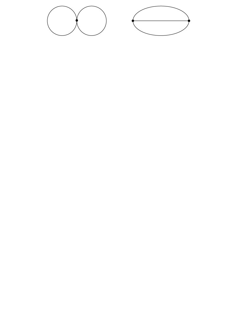
Figure 1: Two-loop supergraphs: ‘eight’ diagram and ‘fish’ diagram.

4.1 Hypermultiplet and ghost supergraphs

We first demonstrate that the two-loop hypermultiplet and ghost quantum corrections cancel each other, for an arbitrary on-shell background ${\cal N}=2$ vector multiplet.

The interactions contained in (2.23) and (2.27) are:

$$S^{(3)}_{{\rm hyper}} = \int{\rm d}\zeta^{(-4)}\,f^{\mu\nu\lambda}\,\breve{q}{}^{+}_{\mu}\,v^{++}_{\nu}\,q^{+}_{\lambda}~{},\qquad S^{(3)}_{\rm ghost}=\int{\rm d}\zeta^{(-4)}\,f^{\mu\nu\lambda}\,({\cal D}^{++}b_{\mu})\,v^{++}_{\nu}\,c_{\lambda}~{},$$ (4.1)

with $f^{\mu\nu\lambda}$ the structure constants. Their combined two-loop contribution,

$${{\rm i}\over 2}\,\Big{\langle}S^{(3)}_{\rm hyper}\,S^{(3)}_{\rm hyper}\Big{\rangle}_{\rm 1PI}+{{\rm i}\over 2}\,\Big{\langle}S^{(3)}_{\rm ghost}\,S^{(3)}_{\rm ghost}\Big{\rangle}_{\rm 1PI}\equiv\Gamma_{\rm I}~{},$$ (4.2)

can be written down in a rather compact form if one notices, following [41, 42],

$${\cal D}^{++}G^{(0,0)}(Z,\,Z^{\prime})=-(u^{+}u^{\prime-})\,G^{(1,1)}(Z,Z^{\prime})~{}.$$ (4.3)

Then one gets

$$\Gamma_{\rm I} = -\frac{1}{2}\int{\rm d}\zeta^{(-4)}\int{\rm d}\zeta^{\prime(-4)}\,f^{\mu\nu\lambda}\,f^{\mu^{\prime}\nu^{\prime}\lambda^{\prime}}\,\Big{\{}1+(u^{+}u^{\prime-})(u^{-}u^{\prime+})\Big{\}}$$ (4.4)

$$\qquad\qquad\times G^{(1,1)}_{\mu\,\mu^{\prime}}(Z,Z^{\prime})\,G^{(1,1)}_{\nu\,\nu^{\prime}}(Z,Z^{\prime})\,G^{(2,2)}_{\lambda\,\lambda^{\prime}}(Z,Z^{\prime})~{}.$$

Use of the identity [41] $1+(u^{+}u^{\prime-})(u^{-}u^{\prime+})=(u^{+}u^{\prime+})(u^{-}u^{\prime-})$ gives

$$\Gamma_{\rm I} = -\frac{1}{2}\int{\rm d}\zeta^{(-4)}\int{\rm d}\zeta^{\prime(-4)}\,f^{\mu\nu\lambda}\,f^{\mu^{\prime}\nu^{\prime}\lambda^{\prime}}\,(u^{+}u^{\prime+})(u^{-}u^{\prime-})$$ (4.5)

$$\qquad\qquad\times G^{(1,1)}_{\mu\,\mu^{\prime}}(Z,Z^{\prime})\,G^{(1,1)}_{\nu\,\nu^{\prime}}(Z,Z^{\prime})\,G^{(2,2)}_{\lambda\,\lambda^{\prime}}(Z,Z^{\prime})~{}.$$

This expression turns out to vanish, due to the presence of $(u^{-}u^{\prime-})$ in the integrand, as we are going to show.

In the case of an arbitrary on-shell ${\cal N}=2$ vector multiplet, the following identity [50] holds

$$[\Delta,({\cal D}^{+})^{4}]=0~{}.$$ (4.6)

This idenity implies

$${\cal D}_{1}^{(ij}\,{\bar{\cal D}}_{1}^{kl)}\,K(z_{1},z_{2}|s)={\cal D}_{2}^{(ij}\,{\bar{\cal D}}_{2}^{kl)}\,K(z_{1},z_{2}|s)~{},$$ (4.7)

and the latter in turn leads [50] (see also [47, 48]) to

$$({\cal D}^{+})^{4}({\cal D}^{\prime+})^{4}\,K(z,z^{\prime}|s) = ({\cal D}^{+})^{4}\Big{\{}(u^{+}u^{\prime+})^{4}\,({\cal D}^{-})^{4}\,-{{\rm i}\over 2}(u^{+}u^{\prime+})^{3}(u^{-}u^{\prime+})\,\Omega^{--}$$ (4.8)

$$\qquad\qquad+(u^{+}u^{\prime+})^{2}(u^{-}u^{\prime+})^{2}\,\Delta\Big{\}}K(z,z^{\prime}|s)~{},$$

where

$$\Omega^{--}={\cal D}^{\alpha{\dot{\alpha}}}{\cal D}^{-}_{\alpha}{\cal D}^{-}_{\dot{\alpha}}+\frac{1}{2}{\cal W}({\cal D}^{-})^{2}+\frac{1}{2}{\bar{\cal W}}({\bar{\cal D}}^{-})^{2}+({\cal D}^{-}{\cal W}){\cal D}^{-}+({\bar{\cal D}}^{-}{\bar{\cal W}}){\bar{\cal D}}^{-}~{}.$$ (4.9)

We thus obtain for the $q$-hypermultiplet propagator

$$G^{(1,1)}(Z,Z^{\prime}) = -{\rm i}(u^{+}u^{\prime+})\int_{0}^{\infty}{\rm d}s\,({\cal D}^{+})^{4}({\cal D}^{-})^{4}\,K(z,z^{\prime}|s)$$ (4.10)

$$-\frac{1}{2}(u^{-}u^{\prime+})\int_{0}^{\infty}{\rm d}s\,({\cal D}^{+})^{4}\Omega^{--}\,K(z,z^{\prime}|s)$$

$$+{(u^{-}u^{\prime+})^{2}\over(u^{+}u^{\prime+})}({\cal D}^{+})^{4}\,\Big{\{}{\bf 1}\delta^{12}(z-z^{\prime})\Big{\}}~{}.$$

As is seen, only the third term in $G^{(1,1)}(Z,Z^{\prime})$ is singular, in the coincidence limit, with respect to the harmonic variables. As concerns the product $(u^{+}u^{\prime+})\,G^{(1,1)}(Z,Z^{\prime})$, it is free of harmonic singularities. Therefore, the only harmonic-singular term in the expression

$$(u^{+}u^{\prime+})\,G^{(1,1)}_{\mu\,\mu^{\prime}}(Z,Z^{\prime})\,G^{(1,1)}_{\nu\,\nu^{\prime}}(Z,Z^{\prime})$$ (4.11)

is proportional to

$$\left(({\cal D}^{+})^{4}\,\Big{\{}{\bf 1}\delta^{12}(z-z^{\prime})\Big{\}}\right)^{2}~{},$$

and this vanishes on considerations of the Grassmann algebra. The non-singular part of (4.11) enters $\Gamma_{\rm I}$ multiplied by

$$(u^{-}u^{\prime-})\,\delta^{(2,-2)}(u,u^{\prime})=0~{}.$$ (4.12)

Therefore, $\Gamma_{\rm I}$ vanishes.

4.2 Gluon ‘fish’ supergraph

The cubic interaction contained in (2.25) is

$$S^{(3)}_{{\rm SYM}} = {{\rm i}\over 3}\,{\rm tr}\,\int{\rm d}^{12}z\int\prod_{a=1}^{3}{\rm d}u_{a}\,\frac{v^{++}(u_{1})v^{++}(u_{2})v^{++}(u_{3})}{(u^{+}_{1}u^{+}_{2})(u^{+}_{2}u^{+}_{3})(u^{+}_{3}u^{+}_{1})}$$ (4.13)

$$= -{1\over 6}\int{\rm d}^{12}z\int\prod_{a=1}^{3}{\rm d}u_{a}\,\frac{f^{\mu\nu\lambda}\,v^{++}_{\mu}(u_{1})v^{++}_{\nu}(u_{2})v^{++}_{\lambda}(u_{3})}{(u^{+}_{1}u^{+}_{2})(u^{+}_{2}u^{+}_{3})(u^{+}_{3}u^{+}_{1})}~{}.$$

It generates a two-loop quantum correction,

$${{\rm i}\over 2}\,\Big{\langle}S^{(3)}_{\rm SYM}\,S^{(3)}_{\rm SYM}\Big{\rangle}_{\rm 1PI}\equiv\Gamma_{\rm II}~{},$$ (4.14)

which can be represented in the form:

$$\Gamma_{\rm II} = -{1\over 12}\int{\rm d}^{12}z\,{\rm d}^{12}z^{\prime}\int\prod_{a=1}^{3}{\rm d}u_{a}\,\prod_{b=1}^{3}{\rm d}u^{\prime}_{b}\,f^{\mu\nu\lambda}\,f^{\mu^{\prime}\nu^{\prime}\lambda^{\prime}}$$ (4.15)

$$\times\frac{G^{(2,2)}_{\mu\,\mu^{\prime}}(z,u_{1};z^{\prime},u^{\prime}_{1})\,G^{(2,2)}_{\nu\,\nu^{\prime}}(z,u_{2};z^{\prime},u^{\prime}_{2})\,G^{(2,2)}_{\lambda\,\lambda^{\prime}}(z,u_{3};z^{\prime},u^{\prime}_{3})}{(u^{+}_{1}u^{+}_{2})(u^{+}_{2}u^{+}_{3})(u^{+}_{3}u^{+}_{1})\,(u^{\prime+}_{1}u^{\prime+}_{2})(u^{\prime+}_{2}u^{\prime+}_{3})(u^{\prime+}_{3}u^{\prime+}_{1})}~{}.$$

For the $U(1)$ gauge background chosen, eq. (2.32), this can be shown, using the group-theoretical results of [18, 19], to reduce to

$$\Gamma_{\rm II} = -{1\over 2}N(N-1)\int{\rm d}^{12}z\,{\rm d}^{12}z^{\prime}\int\prod_{a=1}^{3}{\rm d}u_{a}\,\prod_{b=1}^{3}{\rm d}u^{\prime}_{b}\,$$ (4.16)

$$\times\frac{{\bf G}^{(2,2)}_{\{0\}}(z,u_{1};z^{\prime},u^{\prime}_{1})\,{\bf G}^{(2,2)}_{\{e\}}(z,u_{2};z^{\prime},u^{\prime}_{2})\,{\bf G}^{(2,2)}_{\{-e\}}(z,u_{3};z^{\prime},u^{\prime}_{3})}{(u^{+}_{1}u^{+}_{2})(u^{+}_{2}u^{+}_{3})(u^{+}_{3}u^{+}_{1})\,(u^{\prime+}_{1}u^{\prime+}_{2})(u^{\prime+}_{2}u^{\prime+}_{3})(u^{\prime+}_{3}u^{\prime+}_{1})}~{}.$$

The expression (4.16) turns out to be free of coinciding harmonic sigularities, therefore it is safe to use the short form of the gluon propagator,

$${\bf G}^{(2,2)}_{\{e\}}(z,u;z^{\prime},u^{\prime}) = ({\cal D}^{+})^{4}{\bf G}_{\{e\}}(z,z^{\prime})\,\delta^{(-2,2)}(u,u^{\prime})~{},$$

$${\bf G}_{\{e\}}(z,z^{\prime}) = {\rm i}\int_{0}^{\infty}{\rm d}s\,{\bf K}_{\{e\}}(z,z^{\prime}|s)~{}.$$ (4.17)

This allows us to rewrite $\Gamma_{\rm II}$ as follows:

$$\Gamma_{\rm II} = -{1\over 2}N(N-1)\int{\rm d}^{12}z\,{\rm d}^{12}z^{\prime}\int\prod_{a=1}^{3}{\rm d}u_{a}\,$$ (4.18)

$$\times\frac{\Big{\{}({\cal D}_{1}^{+})^{4}{\bf G}_{\{0\}}(z,z^{\prime})\Big{\}}\Big{\{}({\cal D}_{2}^{+})^{4}{\bf G}_{\{e\}}(z,z^{\prime})\Big{\}}({\cal D}_{3}^{+})^{4}{\bf G}_{\{-e\}}(z,z^{\prime})}{(u^{+}_{1}u^{+}_{2})^{2}(u^{+}_{2}u^{+}_{3})^{2}(u^{+}_{3}u^{+}_{1})^{2}}$$

$$= -{1\over 2}N(N-1)\int{\rm d}^{12}z\,{\rm d}^{12}z^{\prime}\int\prod_{a=1}^{3}{\rm d}u_{a}\,{\bf G}_{\{0\}}(z,z^{\prime})$$

$$\times({\cal D}_{1}^{+})^{4}\,\frac{\Big{\{}({\cal D}_{2}^{+})^{4}{\bf G}_{\{e\}}(z,z^{\prime})\Big{\}}({\cal D}_{3}^{+})^{4}{\bf G}_{\{-e\}}(z,z^{\prime})}{(u^{+}_{1}u^{+}_{2})^{2}(u^{+}_{2}u^{+}_{3})^{2}(u^{+}_{3}u^{+}_{1})^{2}}~{},$$

where the operators $({\cal D}^{+}_{a})^{4}$, with $a=1,2,3$, correspond to the same superspace point $z$, but different harmonics $u^{+}_{a}$. The propagator ${\bf G}_{\{0\}}(z,z^{\prime})$ in this expression is free massless,

$${\bf G}_{\{0\}}(z,z^{\prime})=\int_{0}^{\infty}\frac{{\rm d}s}{(4\pi s)^{2}}\,\,{\rm e}^{\frac{{\rm i}}{4s}\rho^{2}}\,\delta^{8}(\theta-\theta^{\prime})~{},\qquad\delta^{8}(\theta-\theta^{\prime})=\delta^{4}(\xi)\,\delta^{4}(\bar{\xi})~{}.$$ (4.19)

Using the Grassmann delta-function contained in ${\bf G}_{\{0\}}(z,z^{\prime})$, we can do one of the two Grassmann integrals in (4.18), say, the integral over $\theta^{\prime}$. After that, the integrand obtained involves the following expression

$$({\cal D}_{1}^{+})^{4}\left(\Big{\{}({\cal D}_{2}^{+})^{4}{\bf G}_{\{e\}}(z,z^{\prime})\Big{\}}({\cal D}_{3}^{+})^{4}{\bf G}_{\{-e\}(z,z^{\prime})}\right)\Big{|}_{\xi={\bar{\xi}}=0}~{}.$$ (4.20)

We are interested in computing holomorphic quantum corrections of the form (1.21). It is therefore sufficient to use the heat kernel (3.24) which involves a Grassmann delta-function $\delta^{4}(\bar{\xi})$. Since each of the two propagators in (4.20) contains such a delta-function, and since

$${\bar{D}}^{n}\,\delta^{4}({\bar{\xi}})|_{{\bar{\xi}}=0}=0~{},\quad n<4~{},\qquad\quad{\bar{D}}^{4}\,\delta^{4}({\bar{\xi}})=1~{},$$ (4.21)

one needs at least eight derivatives $\bar{\cal D}$’s in order to annihilate the delta-functions in the coincidence limit. However $({\cal D}^{+})^{4}={1\over 16}({\cal D}^{+})^{2}\,({\bar{\cal D}}^{+})^{2}$, and therefore (4.20) contains only six derivatives $\bar{\cal D}$’s. We thus conclude that $\Gamma_{\rm II}$ does not produce quantum corrections of the form (1.21). This clearly disagrees with [30].

4.3 Gluon ‘eight’ supergraph

The quartic interaction contained in (2.25) is

$$S^{(4)}_{{\rm SYM}} = {1\over 4}\,{\rm tr}\,\int{\rm d}^{12}z\int\prod_{a=1}^{4}{\rm d}u_{a}\frac{v^{++}(u_{1})v^{++}(u_{2})v^{++}(u_{3})v^{++}(u_{4})}{(u^{+}_{1}u^{+}_{2})(u^{+}_{2}u^{+}_{3})(u^{+}_{3}u^{+}_{4})(u^{+}_{4}u^{+}_{1})}~{}.$$ (4.22)

It generates the two-loop quantum correction

$$\Gamma_{\rm III}=\Big{\langle}S^{(4)}_{\rm SYM}\,\Big{\rangle}=-\frac{1}{2}\,{\rm tr}(T^{\mu}T^{\nu}T^{\lambda}T^{\sigma})\int{\rm d}^{12}z\int\prod_{a=1}^{4}u_{a}$$ (4.23)

$$\times\left\{\frac{G^{(2,2)}_{\mu\,\nu}(z,u_{1};z,u_{2})\,G^{(2,2)}_{\lambda\,\sigma}(z,u_{3};z,u_{4})}{(u^{+}_{1}u^{+}_{2})(u^{+}_{2}u^{+}_{3})(u^{+}_{3}u^{+}_{4})(u^{+}_{4}u^{+}_{1})}+\frac{1}{2}\frac{G^{(2,2)}_{\mu\,\lambda}(z,u_{1};z,u_{3})\,G^{(2,2)}_{\nu\,\sigma}(z,u_{2};z,u_{4})}{(u^{+}_{1}u^{+}_{2})(u^{+}_{2}u^{+}_{3})(u^{+}_{3}u^{+}_{4})(u^{+}_{4}u^{+}_{1})}\right\}~{}.$$

The second term in (4.23) can be seen to be free of coinciding harmonic sigularities. When computing this term, it is therefore safe to use the short form of $G^{(2,2)}$, eq. (3.3), for the two Green functions involved. We are only interested in computing holomorphic quantum corrections of the form (1.21). It is therefore sufficient to use the heat kernel (3.24) which involves a Grassmann delta-function $\delta^{4}(\bar{\xi})$. Due to (4.21), it is then clear that the second term in (4.23) does not generate any quantum corrections of the form (1.21).

The remaining part of the supergraph under consideration

$$\Gamma^{\prime}_{\rm III} = -\frac{1}{2}\,{\rm tr}(T^{\mu}T^{\nu}T^{\lambda}T^{\sigma})\int{\rm d}^{12}z\int\prod_{a=1}^{4}u_{a}\frac{G^{(2,2)}_{\mu\,\nu}(z,u_{1};z,u_{2})\,G^{(2,2)}_{\lambda\,\sigma}(z,u_{3};z,u_{4})}{(u^{+}_{1}u^{+}_{2})(u^{+}_{2}u^{+}_{3})(u^{+}_{3}u^{+}_{4})(u^{+}_{4}u^{+}_{1})}$$ (4.24)

contains coinciding harmonic sigularities, and therefore we have to use the longer form of $G^{(2,2)}$, eq. (3.4), in order to resolve the singularities.

In accordance with eq. (4.8), we have

$$\frac{({\cal D}^{+})^{4}({\cal D}^{\prime+})^{4}\,K(z,z^{\prime}|s)}{(u^{+}u^{\prime+})}\,({\cal D}^{--})^{2}\,\delta^{(2,-2)}(u,u^{\prime})$$

$$\qquad=({\cal D}^{+})^{4}({\cal D}^{-})^{4}\,K(z,z^{\prime}|s)\,(u^{+}u^{\prime+})^{3}({\cal D}^{--})^{2}\,\delta^{(2,-2)}(u,u^{\prime})$$

$$\qquad\quad-{{\rm i}\over 2}({\cal D}^{+})^{4}\Omega^{--}\,K(z,z^{\prime}|s)(u^{-}u^{\prime+})(u^{+}u^{\prime+})^{2}({\cal D}^{--})^{2}\,\delta^{(2,-2)}(u,u^{\prime})$$

$$\qquad\quad+({\cal D}^{+})^{4}\Delta K(z,z^{\prime}|s)\,(u^{-}u^{\prime+})^{2}(u^{+}u^{\prime+})({\cal D}^{--})^{2}\,\delta^{(2,-2)}(u,u^{\prime})$$ (4.25)

Since ${\cal D}^{--}(u^{+}u^{\prime+})=(u^{-}u^{\prime+})$ and $(u^{+}u^{\prime+})\,\delta^{(2,-2)}=0$, the first term on the right vanishes. The rest can be rewritten as follows

$$\frac{({\cal D}^{+})^{4}({\cal D}^{\prime+})^{4}\,K(z,z^{\prime}|s)}{(u^{+}u^{\prime+})}\,({\cal D}^{--})^{2}\,\delta^{(2,-2)}(u,u^{\prime})$$

$$\qquad=-{\rm i}({\cal D}^{+})^{4}\left\{\Omega^{--}\,K(z,z^{\prime}|s)-2{\partial\over\partial s}K(z,z^{\prime}|s)\,{\cal D}^{--}\right\}\delta^{(-1,1)}(u,u^{\prime})~{},$$ (4.26)

where we have used the heat kernel equation and the identity $(u^{-}u^{\prime+})^{3}\,\delta^{(2,-2)}(u,u^{\prime})=\delta^{(-1,1)}(u,u^{\prime})$. We are only interested in computing holomorphic quantum corrections of the form (1.21). It is therefore sufficient to use the heat kernel (3.24). Since the relation (3.25) holds for this heat kernel, from (4.26) we deduce

$$\frac{({\cal D}^{+})^{4}({\cal D}^{\prime+})^{4}\,K(z,z^{\prime}|s)}{(u^{+}u^{\prime+})}\,({\cal D}^{--})^{2}\,\delta^{(2,-2)}(u,u^{\prime})\Big{|}_{z^{\prime}=z}$$

$$\qquad\qquad\qquad=-{\rm i}\,\delta^{(-1,1)}(u,u^{\prime})\,({\cal D}^{+})^{4}\Omega^{--}\,K(z,z^{\prime}|s)\Big{|}_{z^{\prime}=z}~{}.$$ (4.27)

This leads to

$$\Gamma^{\prime}_{\rm III} = \frac{1}{2}\,{\rm tr}(T^{\mu}T^{\nu}T^{\lambda}T^{\sigma})\int{\rm d}^{12}z\int{\rm d}u_{1}{\rm d}u_{2}\,\frac{{\cal L}^{++}_{\mu\nu}(z,u_{1})\,{\cal L}^{++}_{\lambda\sigma}(z,u_{2})}{(u^{+}_{1}u^{+}_{2})^{2}}~{},$$ (4.28)

where

$${\cal L}^{++}(z,u)={{\rm i}\over 2}\int_{0}^{\infty}{\rm d}s\,s\,({\cal D}^{+})^{4}\Omega^{--}\,K(z,z^{\prime}|s)\Big{|}_{z^{\prime}=z}~{}.$$ (4.29)

Finally, specifying (4.28) to the case of the $U(1)$ background (2.32) gives

$$\Gamma^{\prime}_{\rm III} = \frac{1}{2}\,N(N-1)\int{\rm d}^{12}z\int{\rm d}u_{1}{\rm d}u_{2}\,\frac{{\bf L}^{++}_{\{e\}}(z,u_{1})\,{\bf L}^{++}_{\{e\}}(z,u_{2})}{(u^{+}_{1}u^{+}_{2})^{2}}~{}.$$ (4.30)

Here ${\bf L}^{++}_{\{e\}}(z,u)$ is obtained from ${\cal L}^{++}(z,u)$ by replacing $K(z,z^{\prime}|s)\to{\bf K}_{\{e\}}(z,z^{\prime}|s)$.

It is almost trivial to calculate ${\cal L}^{++}(z,u)$ for the heat kernel (3.24). Indeed, since

$$({\cal D}^{+})^{4}={1\over 16}({\cal D}^{+})^{2}\,({\bar{\cal D}}^{+})^{2}~{},$$

and since the heat kernel (3.24) involves the Grassmann delta-function

$$\delta^{4}({\bar{\xi}})=({\bar{\xi}}^{+})^{2}\,({\bar{\xi}}^{-})^{2}~{},$$

with the properties

$${\bar{\cal D}}^{n}\,\delta^{4}({\bar{\xi}})|_{{\bar{\xi}}=0}=0~{},\quad n<4~{},\qquad\quad{1\over 16}({\bar{\cal D}}^{+})^{2}\,({\bar{\cal D}}^{-})^{2}\,\delta^{4}({\bar{\xi}})=1~{},$$

it is only the third term in the operator $\Omega^{--}$, eq. (4.9), which provides a non-vanishing contribution to ${\cal L}^{++}(z,u)$. It then remains to evaluate

$${1\over 4}({\cal D}^{+})^{2}\,\Big{\{}\delta^{4}(\xi(s))\,I(z,z^{\prime})\Big{\}}\Big{|}_{z^{\prime}=z}~{},\qquad\delta^{4}(\xi(s))=(\xi^{+}(s))^{2}\,(\xi^{-}(s))^{2}~{}.$$

Using the properties of the parallel displacement propagator (see Appendix C)

$$I(z,z)={\bf 1}~{},\qquad{\cal D}^{+}_{\alpha}I(z,z^{\prime})\Big{|}_{z^{\prime}=z}=({\cal D}^{+})^{2}I(z,z^{\prime})\Big{|}_{z^{\prime}=z}=0~{},$$ (4.31)

and the identities (3.18)–(3.20), we obtain

$${\cal L}^{++}(z,u)={1\over 4(4\pi)^{2}}({\cal D}^{+}{\cal W})^{2}\,{\bar{\cal W}}\int_{0}^{\infty}{\rm d}s\,s\,{\rm e}^{-s{\bar{\cal W}}{\cal W}}~{},$$ (4.32)

where the proper-time integral has been Wick-rotated. The expression for ${\cal L}^{++}$ obtained is so simple due to the relation

$${\bf det}\left(\frac{s{\cal F}}{\sinh(s{\cal F})}\right)^{1\over 2}\,(\xi^{+}(s))^{2}\Big{|}_{\xi=0}={s^{2}\over 4}\,({\cal D}^{+}{\cal W})^{2}$$ (4.33)

that holds for the heat kernel (3.24).

Replacing ${\cal W}\to e\,W$ in (4.32) gives

$${\bf L}^{++}_{\{e\}}(z,u)={1\over 4(4\pi)^{2}}\,\sqrt{{N-1\over N}}\,\frac{(D^{+}W)^{2}}{W^{2}{\bar{W}}}~{},$$ (4.34)

where we have inserted the expression for $e$. Now, eqs. (1.21), (4.30) and (4.34) lead to the final result (1.13)

5 Discussion

Using the ${\cal N}=2$ off-shell formulation for ${\cal N}=4$ SYM in harmonic superspace, in this paper we computed the two-loop quantum correction to the holomorphic sector $\Lambda({\bar{\Psi}})$ of the low-energy effective action (1.7). Relation (1.13) is our main result. As explained in section 1, the explicit structure of $\Lambda_{\rm two-loop}({\bar{\Psi}})$ is consistent with the self-duality equations (1.5) and (1.6), as well as with the conjectured correspondence between the D3-brane action in $AdS_{5}\times S^{5}$ and the low-energy effective action for ${\cal N}=4$ $SU(N)$ SYM with the gauge group spontaneously broken to $SU(N-1)\times U(1)$.

It is a by-product of our calculation that no quantum correction to the $c$-term in (1.7) is generated in ${\cal N}=4$ SYM at the two-loop level. This is consistent with the Dine-Seiberg non-renormalization conjecture [17] and its generalized form [18, 19]. The absence of two-loop $F^{4}$ quantum corrections was also established in [19] using the ${\cal N}=1$ superfield formulation for ${\cal N}=4$ SYM. It should be pointed out that two-loop $F^{4}$ contributions are actually generated from both the hypermultiplet and ghost ‘fish’ supergraphs. But in the case of ${\cal N}=4$ SYM, the hypermultiplet and ghost contributions cancel each other at two loops, in accordance with the consideration in subsection 4.1.

Apart from the analysis given in the present paper, two independent calculations of the two-loop $F^{6}$ quantum correction in ${\cal N}=4$ SYM have been carried out [30, 19]. They were based, respectively, on the use of (i) ${\cal N}=2$ harmonic supergraphs [30]; and (ii) ${\cal N}=1$ supergraphs [19]. Unfortunately, there is no agreement between the results of the three calculations given.

It is not difficult to compare the outcome of our calculation with that of [30], as well as to figure out the origin of differences. Referring to eq. (1.17), the result of our calculation corresponds to the choice $\kappa_{1}$, while the calculation in [30] leads to $\kappa_{2}$. Comparing the technical blocks of our calculation with [30], the results prove to differ in the sectors of the ‘fish’ and ‘eight’ gluon diagrams. In our approach, there is no contribution from the ‘fish,’ and the entire quantum correction comes from the ‘eight’ diagram. According to [30], the situation is just opposite – the entire quantum correction comes from the ‘fish’ supergraph. We believe that the calculation in [30] is not correct. When evaluating two-loop harmonic supergraphs, it turns out that a crucial role is played by the identity (4.8) (or its equivalent form originally given in [47, 48]) which allows one to resolve coinciding harmonic singularities. Although this identity had been known at the time, it was not taken into account in [30]. Unfortunately, the notoriously difficult problem of coinciding harmonic singularities [52, 24, 47, 48, 54] is the high price one has to pay for the indispensable advantage of manifest ${\cal N}=2$ supersymmetry in the quantum harmonic superspace approach. This is the technical problem which has no analogue in ${\cal N}=1$ superspace and which all quantum practitioners face, sooner or later, once engaged with harmonic supergraphs (the founding fathers of harmonic superspace have only considered a few simple examples of singular harmonic supergraphs [52, 42]). At the one-loop level, the problem of coinciding harmonic singularities was solved in [24, 47, 48]. But it then emerged again at two loops [30, 54]. Now we believe, on the basis of the experience gained and the analysis given in this paper and also in [54], that the two-loop approximation is under control. However, three loops may bring a new challenge. It would, therefore, be very important to formulate well-defined rules to resolve coinciding singularities in harmonic supergraphs at any loop order.

According to the ${\cal N}=1$ supergraph considerations in [19], no two-loop $F^{6}$ quantum correction is generated in ${\cal N}=4$ SYM. This is not compatible with the correspondence between the D3-brane action in $AdS_{5}\times S^{5}$ and the low-energy action for ${\cal N}=4$ SYM, provided one naively identifies the component fields of the ${\cal N}=2$ vector multiplet $(\phi,W_{\alpha})$ with those living on the D3-brane. But most likely, such an identification is not consistent, as was discussed in the Introduction.

The two-loop $F^{6}$ results of [19] and of the present paper do not match so far. This discrepancy may be due to the fact that, in the process of background-field quantization, different gauge conditions were used in [19] and in the present paper (in particular, the gauge condition in [19] respected only the ${\cal N}=1$ supersymmetry). Unlike the $S$-matrix, which is determined by the effective action at its stationary point, the off-shell effective action in gauge theories is known to depend on the choice of gauge conditions. As shown, e.g., in [55], the one-loop effective action evaluated at a classical stationary point (the on-shell $U(1)$ vector multiplet in our case) is gauge independent. At the same classical stationary point, the two-loop effective action becomes gauge independent only after adding up some one-particle reducible functional generated by the one-loop action. For different gauge conditions, the corresponding effective actions are related by a field redefinition. The $F^{6}$ term and higher order terms may be sensitive to such field redefinitions. Due to its importance, let us try to make this point a bit more precise.

For a gauge theory of Yang-Mills type, let $\Gamma[\varphi]$ be the gauge-invariant effective action defined in the framework of background-field quantization,

$$\Gamma[\varphi]=S[\varphi]+\sum_{L=1}^{\infty}\hbar^{L}\Gamma^{(L)}[\varphi]~{},$$ (5.1)

with $S[\varphi]$ the classical action, and $\Gamma^{(L)}[\varphi]$ the $L$-loop quantum correction. At a generic point $\varphi^{i}$, the effective action explicitly depends on the gauge conditions used in the process of the Faddeev-Popov quantization. This dependence disappears at the stationary point of the effective action

$$\Gamma_{,i}[\hat{\varphi}]=0~{},\qquad\hat{\varphi}=\varphi_{0}+\hbar\varphi^{(1)}+\hbar^{2}\varphi^{(2)}+\cdots~{},$$ (5.2)

with $\varphi_{0}$ the classical stationary point, $S_{,i}[\varphi_{0}]=0$. More precisely, it is $\Gamma[\hat{\varphi}]$ which does not depend on the gauge conditions chosen, but both $\Gamma[\varphi]$ and $\hat{\varphi}$ are “gauge-dependent.” It can be shown [55] that the one-loop effective action evaluated at the classical stationary point, $\Gamma^{(1)}[\varphi_{0}]$, does not depend on the gauge conditions chosen, but this is no longer true for the two-loop quantum correction $\Gamma^{(2)}[\varphi_{0}]$. Now, in the case of ${\cal N}=4$ SYM, the corresponding formulations in ${\cal N}=1$ superspace and in ${\cal N}=2$ superspace require different gauge conditions. For this theory, there exists perfect agreement between $\Gamma^{(1)}[\varphi_{0}]$ evaluated in terms of ${\cal N}=1$ superfields [13] and ${\cal N}=2$ superfields [47]. But the two-loop quantum corrections should not necessarily coincide. Their relationship will be studied in a separate publication.

Of course, if there exists an exact solution to all orders, $\hat{\varphi}=\varphi_{0}$, then $\Gamma[\varphi_{0}]$ does not depend on the gauge conditions chosen. This is what happens in QED where any constant field configuration, $F_{mn}={\rm const}$, is an exact solution for the Euler-Heisenberg effective action. The situation is different in the case of the ${\cal N}=4$ SYM effective action (1.7). An ${\cal N}=2$ supersymmetric generalization of $F_{mn}={\rm const}$ is

$${\bar{D}}^{i}_{\dot{\alpha}}W=D^{i}_{\alpha}{\bar{W}}=D^{ij}W={\bar{D}}^{ij}{\bar{W}}=\partial_{a}W=\partial_{a}{\bar{W}}=0~{},$$ (5.3)

with $F$ associated with the component $D^{i}{}_{\alpha}D_{\beta i}W|_{\theta=0}$ and its conjugate. Such a superfield is a solution for the classical $U(1)$ vector multiplet action (1.8). However, once we replace $S_{\rm cl}$ by the action (1.18), which contains the leading quantum correction, the configuration (5.3) is no longer a solution. This can be seen by inspecting the equation of motion

$$(D^{+})^{2}F^{\prime}(W)+({\bar{D}}^{+})^{2}{\bar{F}}^{\prime}({\bar{W}})+(D^{+})^{4}\left\{({\bar{D}}^{-})^{2}\frac{\partial}{\partial W}+(D^{-})^{2}\frac{\partial}{\partial\bar{W}}\right\}H(W,{\bar{W}})=0$$ (5.4)

corresponding to the action

$$I=2\,{\rm Re}\int{\rm d}^{8}z\,F(W)+\int{\rm d}^{12}z\,H(W,{\bar{W}})~{}.$$ (5.5)

Thus, quantum corrections deform the classical superfield solution (5.3). This is actually expected keeping in mind the correspondence between the D3-brane action (1.14) and the ${\cal N}=4$ SYM effective action. Indeed, it was mentioned in the Introduction that the only constant field solutions for the D3-brane in $AdS_{5}\times S^{5}$ are $F_{mn}=0$ and $X^{I}={\rm const}$, although the quadratic part of the D3-brane action (1.14) possesses more general solutions: $F_{mn}={\rm const}$ and $X^{I}={\rm const}$.

In fact, there exists a simple exact solution for the low-energy effective action (1.7):

$${\bar{D}}^{i}_{\dot{\alpha}}W=D^{ij}W=\partial_{a}W=0~{},\qquad{\bar{W}}={\rm const}~{}.$$ (5.6)

Its use should in principle be enough to uniquely restore the holomorphic $\Lambda$-term in (1.7) which clearly indicates that this $\Lambda$-term is gauge-independent. It is important to note that such a solution allows us to extract nontrivial information about the effective action only in the ${\cal N}=2$ superspace setting (when reduced to ${\cal N}=1$ superspace, the effective action trivializes unless we relax the constraints on $\bar{W}$ to ${\bar{D}}^{i}_{\dot{\alpha}}{\bar{W}}\neq 0$). This may be the origin of the discrepancy between the ${\cal N}=1$ [19] and ${\cal N}=2$ results. In Minkowski space, the conditions (5.6) are of course purely formal, as they are obviously inconsistent with the structure of a single real vector multiplet. But the use of complex field configurations is completely legitimate when we are interested in special sectors of the effective action, see, e.g., [60].

Acknowledgements:
It is the pleasure to thank Ian McArthur for numerous discussions and for collaboration at early stages of this project. The author is grateful to Ioseph Buchbinder and especially to Arkady Tseytlin for reading the manuscript and for important critical comments and suggestions. This work is supported in part by the Australian Research Council.

Appendix A Superspace integration measures

Here we introduce various ${\cal N}=2$ superspace integration measures used throughout this paper. They are defined in terms of the spinor covariant derivatives $D^{i}_{\alpha}$ and ${\bar{D}}^{\dot{\alpha}}_{i}$, with $i=\hat{1},\hat{2}$, and the related fourth-order operators

$$D^{4}={1\over 16}(D^{\hat{1}})^{2}(D^{\hat{2}})^{2}={1\over 48}D^{ij}D_{ij}~{},\qquad{\bar{D}}^{4}={1\over 16}({\bar{D}}_{\hat{1}})^{2}({\bar{D}}_{\hat{2}})^{2}={1\over 48}{\bar{D}}^{ij}{\bar{D}}_{ij}~{},$$ (A.1)

where the second-order operators $D^{ij}$ and ${\bar{D}}^{ij}$ are given in (1.1). Integration over the chiral subspace is defined by

$$\int{\rm d}^{8}z\,L_{\rm c}=\int{\rm d}^{4}x\,D^{4}L_{\rm c}~{},\qquad{\bar{D}}^{i}_{\dot{\alpha}}L_{\rm c}=0~{}.$$ (A.2)

Integration over the full superspace is defined by

$$\int{\rm d}^{12}z\,L=\int{\rm d}^{4}x\,{\bar{D}}^{4}D^{4}L~{}.$$ (A.3)

In terms of the harmonic-dependent spinor derivatives $D^{\pm}_{\alpha}=D^{i}_{\alpha}\,u^{\pm}_{i}$ and ${\bar{D}}^{\pm}_{\dot{\alpha}}={\bar{D}}^{i}_{\dot{\alpha}}\,u^{\pm}_{i}$, and the related fourth-order operators

$$(D^{+})^{4}={1\over 16}(D^{+})^{2}({\bar{D}}^{+})^{2}~{},\qquad(D^{-})^{4}={1\over 16}(D^{-})^{2}({\bar{D}}^{-})^{2}~{},$$ (A.4)

integration over the analytic subspace is defined by

$$\int{\rm d}\zeta^{(-4)}\,L^{(+4)}=\int{\rm d}^{4}x\int{\rm d}u\,(D^{-})^{4}L^{(+4)}~{},\qquad D^{+}_{\alpha}L^{(+4)}={\bar{D}}^{+}_{\dot{\alpha}}L^{(+4)}=0~{}.$$ (A.5)

Integration over the group manifold $SU(2)$ is defined according to [40]

$$\int{\rm d}u\,1=1~{}\qquad\int{\rm d}u\,u^{+}_{(i_{1}}\cdots u^{+}_{i_{n}}\,u^{-}_{j_{1}}\cdots u^{-}_{j_{m})}=0~{},\quad n+m>0~{}.$$ (A.6)

Appendix B Group-theoretical results

Here we describe the $SU(N)$ conventions adopted in the paper. Lower-case Latin letters from the middle of the alphabet, $i,j,\dots$, will be used to denote matrix elements in the fundamental, with the convention $i=0,1,\dots,N-1\equiv 0,\underline{i}$. We choose a Cartan-Weyl basis to consist of the elements:

$$H^{I}=\{H^{0},H^{\underline{I}}\}~{},\quad\underline{I}=1,\dots,N-2~{},\qquad\quad E^{ij}~{},\quad i\neq j~{}.$$ (B.1)

The basis elements in the fundamental representation are defined similarly to [56],

$$(E^{ij})^{kl} = \delta^{ik}\,\delta^{jl}~{},$$

$$(H^{I})^{kl} = \frac{1}{\sqrt{(N-I)(N-I-1)}}\Big{\{}(N-I)\,\delta^{kI}\,\delta^{lI}-\sum\limits_{i=I}^{N-1}\delta^{ki}\,\delta^{li}\Big{\}}~{},$$ (B.2)

and are characterized by the properties

$${\rm tr}(H^{I}\,H^{J})=\delta^{IJ}~{},\qquad{\rm tr}(E^{ij}\,E^{kl})=\delta^{il}\,\delta^{jk}~{},\qquad{\rm tr}(H^{I}\,E^{kl})=0~{}.$$ (B.3)

A generic element of the Lie algebra $su(N)$ is

$$v=v_{I}\,H^{I}+v_{ij}\,E^{ij}\equiv v_{\mu}\,T^{\mu}~{},\qquad i\neq j~{},$$ (B.4)

For $SU(N)$, the operation of trace in the adjoint representation, ${\rm tr}_{\rm Ad}$, is related to that in the fundamental, ${\rm tr}$, as follows

$${\rm tr}_{\rm Ad}\,v^{2}=2N\,{\rm tr}\,v^{2}~{},\qquad v\in su(N)~{}.$$ (B.5)

Since the basis (B.1) is not orthonormal, ${\rm tr}(T^{\mu}\,T^{\nu})=g^{\mu\nu}\neq\delta^{\mu\nu}$, it is necessary to keep track of the Cartan-Killing metric when working with adjoint vectors. For any elements $u=u_{\mu}T^{\mu}$ and $v=v_{\mu}T^{\mu}$ of the Lie algebra, we have $u\cdot v={\rm tr}(u\,v)=u_{\mu}\,v^{\mu}$, where $v^{\mu}=g^{\mu\nu}v_{\nu}$ ($v^{I}=v_{I}$, $v^{ij}=v_{ji}$). The structure constants of $SU(N)$ are defined in a standard way, $[T^{\mu},T^{\nu}]={\rm i}\,f^{\mu\nu}{}_{\lambda}T^{\lambda}={\rm i}\,f^{\mu\nu\lambda}T_{\lambda}$.

Appendix C Parallel displacement propagator

In this appendix we describe, basically following [57], the main properties of the parallel displacement propagator $I(z,z^{\prime})$ in ${\cal N}=2$ superspace. This object is uniquely specified by the following requirements:
(i) the gauge transformation law

$$I(z,z^{\prime})~{}\to~{}{\rm e}^{{\rm i}\tau(z)}\,I(z,z^{\prime})\,{\rm e}^{-{\rm i}\tau(z^{\prime})}~{}$$ (C.1)

with respect to the gauge ($\tau$-frame) transformation of the covariant derivatives (2.2);
(ii) the equation

$$\Xi^{A}{\cal D}_{A}\,I(z,z^{\prime})=\Xi^{A}\Big{(}D_{A}+{\rm i}\,{\cal V}_{A}(z)\Big{)}I(z,z^{\prime})=0~{};$$ (C.2)

(iii) the boundary condition

$$I(z,z)={\bf 1}~{}.$$ (C.3)

These imply the important relation

$$I(z,z^{\prime})\,I(z^{\prime},z)={\bf 1}~{},$$ (C.4)

as well as

$$\Xi^{A}{\cal D}^{\prime}_{A}\,I(z,z^{\prime})=\Xi^{A}\Big{(}D^{\prime}_{A}\,I(z,z^{\prime})-{\rm i}\,I(z,z^{\prime})\,{\cal V}_{A}(z^{\prime})\Big{)}=0~{}.$$ (C.5)

Let $\Psi(z)$ be a harmonic-independent superfield transforming in some representation of the gauge group,

$$\Psi(z)~{}\to~{}{\rm e}^{{\rm i}\tau(z)}\,\Psi(z)~{}.$$ (C.6)

Then it can be represented by the covariant Taylor series [57]

$$\Psi(z)=I(z,z^{\prime})\,\sum_{n=0}^{\infty}{1\over n!}\,\Xi^{A_{n}}\ldots\Xi^{A_{1}}\,{\cal D}^{\prime}_{A_{1}}\ldots{\cal D}^{\prime}_{A_{n}}\,\Psi(z^{\prime})~{}.$$ (C.7)

The fundametal properties of the parallel displacement propagator are [57]

$${\cal D}_{B}I(z,z^{\prime}) = {\rm i}\,I(z,z^{\prime})\,\sum_{n=1}^{\infty}{1\over(n+1)!}\,\Big{\{}n\,\Xi^{A_{n}}\ldots\Xi^{A_{1}}{\cal D}^{\prime}_{A_{1}}\ldots{\cal D}^{\prime}_{A_{n-1}}{\cal F}_{A_{n}\,B}(z^{\prime})$$

$$+ \frac{1}{2}(n-1)\,\Xi^{A_{n}}T_{A_{n}\,B}{}^{C}\,\Xi^{A_{n-1}}\ldots\Xi^{A_{1}}{\cal D}^{\prime}_{A_{1}}\ldots{\cal D}^{\prime}_{A_{n-2}}{\cal F}_{A_{n-1}\,C}(z^{\prime})\Big{\}}~{},$$

and

$${\cal D}_{B}I(z,z^{\prime}) = {\rm i}\,\sum_{n=1}^{\infty}{(-1)^{n}\over(n+1)!}\,\Big{\{}-\Xi^{A_{n}}\ldots\Xi^{A_{1}}{\cal D}_{A_{1}}\ldots{\cal D}_{A_{n-1}}{\cal F}_{A_{n}\,B}(z)$$

$$+ \frac{1}{2}(n-1)\,\Xi^{A_{n}}T_{A_{n}\,B}{}^{C}\,\Xi^{A_{n-1}}\ldots\zeta^{A_{1}}{\cal D}_{A_{1}}\ldots{\cal D}_{A_{n-2}}{\cal F}_{A_{n-1}\,C}(z)\Big{\}}\,I(z,z^{\prime})~{}.$$

Here ${\cal F}_{AB}$ denotes the superfield strength defined as follows

$$[{\cal D}_{A},{\cal D}_{B}\}=T_{AB}{}^{C}{\cal D}_{C}+{\rm i}\,{\cal F}_{AB}~{}.$$ (C.10)

In the case of a covariantly constant vector multiplet, the series in (C) and (C) terminate as only the tensors ${\cal F}_{CD}$, ${\cal D}_{A}{\cal F}_{CD}$ and ${\cal D}_{A}{\cal D}_{B}{\cal F}_{CD}$ have non-vanishing components.

The parallel displacement propagator in the $\lambda$-frame is obtained from that in the $\tau$-frame by the transformation

$$I(z,z^{\prime})\equiv I_{\tau}(z,z^{\prime})\quad\longrightarrow\quad{\rm e}^{{\rm i}\Omega(z,u)}\,I(z,z^{\prime})\,{\rm e}^{-{\rm i}\Omega(z^{\prime},u^{\prime})}\equiv I_{\lambda}(Z,Z^{\prime})~{},$$ (C.11)

with $Z=\{z,u\}$.

Appendix D Free propagators

Following [58], introduce a generalization of the supersymmetric two-point function $\rho(z,z^{\prime})$, eq. (3.11),

$$\hat{\rho}^{a} = \hat{\rho}^{a}(Z,Z^{\prime})=-\hat{\rho}^{a}(Z^{\prime},Z)=\rho^{a}-2{\rm i}\,\frac{u^{+}_{(i}u^{\prime+}_{j)}\,\xi^{i}\sigma^{a}{\bar{\xi}}^{j}}{(u^{+}u^{\prime+})}~{}.$$ (D.1)

It follows from (3.14)

$$D^{+}_{\beta}\hat{\rho}^{a}=D^{\prime+}_{\beta}\hat{\rho}^{a}=0~{},\qquad{\bar{D}}^{+}_{\dot{\beta}}\hat{\rho}^{a}={\bar{D}}^{\prime+}_{\dot{\beta}}\hat{\rho}^{a}=0~{}.$$ (D.2)

Thus the two-point function introduced is analytic with respect to $Z$ and $Z^{\prime}$, and therefore it can be represented in the form $\hat{\rho}^{a}=\hat{\rho}^{a}(\zeta,\zeta^{\prime})=-\hat{\rho}^{a}(\zeta^{\prime},\zeta)$, where the variables $\zeta=(y^{a},\theta^{+\alpha},{\bar{\theta}}^{+}_{\dot{\alpha}},\,u^{+}_{i},u^{-}_{j})$ parametrize the analytic subspace of harmonic superspace. The result can be found, e.g., in [42].

With the use of (D.1), the free massless heat kernel can be written in two equivalent form

$$K(z,z^{\prime}|s) = -\frac{\rm i}{(4\pi s)^{2}}\,\,{\rm e}^{\frac{{\rm i}}{4s}\rho^{2}}\,\delta^{4}(\xi)\,\delta^{4}(\bar{\xi})=-\frac{\rm i}{(4\pi s)^{2}}\,\,{\rm e}^{\frac{{\rm i}}{4s}\hat{\rho}^{2}}\,\delta^{4}(\xi)\,\delta^{4}(\bar{\xi})~{}.$$ (D.3)

Since $\hat{\rho}^{2}$ is analytic at $Z$ and $Z^{\prime}$, we obtain

$$(D^{+})^{4}(D^{\prime+})^{4}\,K(z,z^{\prime}|s) = -\frac{\rm i}{(4\pi s)^{2}}\,\,{\rm e}^{\frac{{\rm i}}{4s}\hat{\rho}^{2}}(D^{+})^{4}(D^{\prime+})^{4}\,\delta^{4}(\xi)\,\delta^{4}(\bar{\xi})$$ (D.4)

$$= -\frac{\rm i}{(4\pi s)^{2}}\,\,{\rm e}^{\frac{{\rm i}}{4s}\hat{\rho}^{2}}(u^{+}u^{\prime+})^{4}~{}.$$

The free massless $q$-hypermultiplet propagator becomes

$$G^{(1,1)}(Z,Z^{\prime}) = -{\rm i}\int_{0}^{\infty}{\rm d}s\,(D^{+})^{4}(D^{\prime+})^{4}\,{K(z,z^{\prime}|s)\over(u^{+}u^{\prime+})^{3}}=-{{\rm i}\over 4\pi^{2}}\,{(u^{+}u^{\prime+})\over\hat{\rho}^{2}+{\rm i}\varepsilon}\Big{|}_{\varepsilon\to+0}~{},$$ (D.5)

and the latter expression for $G^{(1,1)}$ was given, e.g., in [42]. A similar, although somewhat uglier, representation follows for the gluon propagator.

Representation (D.5) is known to be extremely useful for computing correlation functions of composite operators in the unbroken phase of ${\cal N}=2,4$ superconformal field theories, see [42] and references therein. It is not clear whether such ideas might be of any use in the case of background-field calculations.

References

• [1] C. Montonen and D. I. Olive, “Magnetic monopoles as gauge particles?,” Phys. Lett. B 72 (1977) 117; H. Osborn, “Topological charges for N=4 supersymmetric gauge theories and monopoles of spin 1,” Phys. Lett. B 83 (1979) 321; A. Sen, “Dyon-monopole bound states, self-dual harmonic forms on the multi-monopole moduli space, and SL(2,Z) invariance in string theory,” Phys. Lett. B 329 (1994) 217 [arXiv:hep-th/9402032].
• [2] N. Seiberg and E. Witten, “Electric - magnetic duality, monopole condensation, and confinement in N=2 supersymmetric Yang-Mills theory,” Nucl. Phys. B 426 (1994) 19 (Erratum-ibid. B 430 (1994) 485) [arXiv:hep-th/9407087]; “Monopoles, duality and chiral symmetry breaking in N=2 supersymmetric QCD,” Nucl. Phys. B 431 (1994) 484 [arXiv:hep-th/9408099].
• [3] J. M. Maldacena, “The large N limit of superconformal field theories and supergravity,” Adv. Theor. Math. Phys.  2 (1998) 231 [arXiv:hep-th/9711200].
• [4] F. Gonzalez-Rey, B. Kulik, I. Y. Park and M. Roček, “Self-dual effective action of N = 4 super-Yang-Mills,” Nucl. Phys. B 544 (1999) 218 [arXiv:hep-th/9810152].
• [5] S. M. Kuzenko and S. Theisen, “Supersymmetric duality rotations,” JHEP 0003 (2000) 034 [arXiv:hep-th/0001068].
• [6] R. Grimm, M. Sohnius and J. Wess, “Extended supersymmetry and gauge theories,” Nucl. Phys. B 133 (1978) 275.
• [7] M. Henningson, “Extended superspace, higher derivatives and SL(2,Z) duality,” Nucl. Phys. B 458 (1996) 445 [arXiv:hep-th/9507135].
• [8] L. Mezincescu, “On the superfield formulation of O(2) supersymmetry,” Dubna preprint JINR-P2-12572, 1979.
• [9] G. W. Gibbons and D. A. Rasheed, “Electric - magnetic duality rotations in nonlinear electrodynamics,” Nucl. Phys. B 454 (1995) 185 [arXiv:hep-th/9506035]; “SL(2,R) invariance of non-linear electrodynamics coupled to an axion and a dilaton,” Phys. Lett. B 365 (1996) 46 [arXiv:hep-th/9509141].
• [10] M. K. Gaillard and B. Zumino, “Self-duality in nonlinear electromagnetism,” in Supersymmetry and Quantum Field Theory, J. Wess and V. P. Akulov (Eds.), Springer, 1998, p. 121 [hep-th/9705226]; “Nonlinear electromagnetic self-duality and Legendre transformations,” in Duality and Supersymmetric Theories, D. I. Olive and P. C. West (Eds.), Cambridge University Press, 1999, p. 33 [hep-th/9712103].
• [11] S. M. Kuzenko and S. Theisen, “Nonlinear self-duality and supersymmetry,” Fortsch. Phys.  49 (2001) 273 [arXiv:hep-th/0007231].
• [12] E. A. Ivanov and B. M. Zupnik, “New representation for Lagrangians of self-dual nonlinear electrodynamics,” arXiv:hep-th/0202203; “New approach to nonlinear electrodynamics: Dualities as symmetries of interaction,” arXiv:hep-th/0303192.
• [13] I. L. Buchbinder, S. M. Kuzenko and A. A. Tseytlin, “On low-energy effective actions in N = 2,4 superconformal theories in four dimensions,” Phys. Rev. D 62 (2000) 045001 [arXiv:hep-th/9911221].
• [14] A. Jevicki, Y. Kazama and T. Yoneya, “Quantum metamorphosis of conformal transformation in D3-brane Yang-Mills theory,” Phys. Rev. Lett.  81 (1998) 5072 [arXiv:hep-th/9808039]; S. M. Kuzenko and I. N. McArthur, “Quantum deformation of conformal symmetry in N = 4 super Yang-Mills theory,” Nucl. Phys. B 640 (2002) 78 [arXiv:hep-th/0203236]; “On quantum deformation of conformal symmetry: Gauge dependence via field redefinitions,” Phys. Lett. B 544 (2002) 357 [arXiv:hep-th/0206234]; S. M. Kuzenko, I. N. McArthur and S. Theisen, “Low energy dynamics from deformed conformal symmetry in quantum 4D N = 2 SCFTs,” Nucl. Phys. B 660 (2003) 131 [arXiv:hep-th/0210007].
• [15] S. M. Kuzenko and S. Theisen, “Correlation functions of conserved currents in N = 2 superconformal theory,” Class. Quant. Grav.  17 (2000) 665 [arXiv:hep-th/9907107].
• [16] B. de Wit, M. T. Grisaru and M. Roček, “Nonholomorphic corrections to the one-loop N=2 super Yang-Mills action,” Phys. Lett. B 374 (1996) 297 [arXiv:hep-th/9601115].
• [17] M. Dine and N. Seiberg, “Comments on higher derivative operators in some SUSY field theories,” Phys. Lett. B 409 (1997) 239 [arXiv:hep-th/9705057].
• [18] S. M. Kuzenko and I. N. McArthur, “On the two-loop four-derivative quantum corrections in 4-D N = 2 superconformal field theories,” Nucl. Phys. B 683 (2004) 3 [arXiv:hep-th/0310025].
• [19] S. M. Kuzenko and I. N. McArthur, “Relaxed super self-duality and N = 4 SYM at two loops,” Nucl. Phys. B 697 (2004) 89 [arXiv:hep-th/0403240].
• [20] M. Matone, “Modular invariance and exact Wilsonian action of N = 2 SYM,” Phys. Rev. Lett.  78 (1997) 1412 [arXiv:hep-th/9610204]; D. Bellisai, F. Fucito, M. Matone and G. Travaglini, “Non-holomorphic terms in N = 2 SUSY Wilsonian actions and RG equation,” Phys. Rev. D 56 (1997) 5218 [arXiv:hep-th/9706099].
• [21] N. Dorey, V. V. Khoze, M. P. Mattis, M. J. Slater and W. A. Weir, “Instantons, higher-derivative terms, and nonrenormalization theorems in supersymmetric gauge theories,” Phys. Lett. B 408 (1997) 213 [arXiv:hep-th/9706007].
• [22] V. Periwal and R. von Unge, “Accelerating D-branes,” Phys. Lett. B 430 (1998) 71 [arXiv:hep-th/9801121].
• [23] F. Gonzalez-Rey and M. Roček, “Nonholomorphic N = 2 terms in N = 4 SYM: 1-loop calculation in N = 2 superspace,” Phys. Lett. B 434 (1998) 303 [arXiv:hep-th/9804010].
• [24] I. L. Buchbinder and S. M. Kuzenko, “Comments on the background field method in harmonic superspace: Non-holomorphic corrections in N = 4 SYM,” Mod. Phys. Lett. A 13 (1998) 1623 [arXiv:hep-th/9804168].
• [25] E. I. Buchbinder, I. L. Buchbinder and S. M. Kuzenko, “Non-holomorphic effective potential in N = 4 SU(n) SYM,” Phys. Lett. B 446 (1999) 216 [arXiv:hep-th/9810239].
• [26] D. A. Lowe and R. von Unge, “Constraints on higher derivative operators in maximally supersymmetric gauge theory,” JHEP 9811 (1998) 014 [arXiv:hep-th/9811017].
• [27] E. S. Fradkin and A. A. Tseytlin, “Quantization and dimensional reduction: One loop results for super Yang-Mills and supergravities in $D\geq 4$,” Phys. Lett. B 123 (1983) 231; “Quantum properties of higher dimensional and dimensionally reduced supersymmetric theories,” Nucl. Phys. B 227 (1983) 252.
• [28] I. Chepelev and A. A. Tseytlin, “Long-distance interactions of branes: Correspondence between supergravity and super Yang-Mills descriptions,” Nucl. Phys. B 515 (1998) 73 [arXiv:hep-th/9709087].
• [29] A. A. Tseytlin, “Born-Infeld action, supersymmetry and string theory,” in M. Shifman (Ed.), The Many Faces of the Superworld, World Scientific, 2000, p. 417, arXiv:hep-th/9908105.
• [30] I. L. Buchbinder, A. Y. Petrov and A. A. Tseytlin, “Two-loop N = 4 super Yang Mills effective action and interaction between D3-branes,” Nucl. Phys. B 621 (2002) 179 [arXiv:hep-th/0110173].
• [31] A. A. Tseytlin, “Self-duality of Born-Infeld action and Dirichlet 3-brane of type IIB superstring theory,” Nucl. Phys. B 469 (1996) 51 [arXiv:hep-th/9602064]; M. B. Green and M. Gutperle, “Comments on three-branes,” Phys. Lett. B 377 (1996) 28 [arXiv:hep-th/9602077].
• [32] S. Cecotti and S. Ferrara, “Supersymmetric Born-Infeld Lagrangians,” Phys. Lett. B 187 (1987) 335.
• [33] J. Bagger and A. Galperin, “A new Goldstone multiplet for partially broken supersymmetry,” Phys. Rev. D 55 (1997) 1091 [arXiv:hep-th/9608177].
• [34] M. Roček and A. A. Tseytlin, “Partial breaking of global D = 4 supersymmetry, constrained superfields, and 3-brane actions,” Phys. Rev. D 59 (1999) 106001 [arXiv:hep-th/9811232].
• [35] D. V. Volkov and V. P. Akulov, “Is the neutrino a Goldstone particle?,” Phys. Lett. B 46 (1973) 109.
• [36] T. Hatanaka and S. V. Ketov, “On the universality of Goldstino action,” Phys. Lett. B 580 (2004) 265 [arXiv:hep-th/0310152].
• [37] S. Bellucci, E. Ivanov and S. Krivonos, “N = 2 and N = 4 supersymmetric Born-Infeld theories from nonlinear realizations,” Phys. Lett. B 502 (2001) 279 [arXiv:hep-th/0012236]; “Towards the complete N = 2 superfield Born-Infeld action with partially broken N = 4 supersymmetry,” Phys. Rev. D 64 (2001) 025014 [arXiv:hep-th/0101195].
• [38] S. M. Kuzenko and I. N. McArthur, “Goldstone multiplet for partially broken superconformal symmetry,” Phys. Lett. B 522 (2001) 320 [arXiv:hep-th/0109183].
• [39] S. Bellucci, E. Ivanov and S. Krivonos, “Goldstone superfield actions for partially broken AdS(5) supersymmetry,” Phys. Lett. B 558 (2003) 182 [arXiv:hep-th/0212142]; “Goldstone superfield actions in AdS(5) backgrounds,” Nucl. Phys. B 672 (2003) 123 [arXiv:hep-th/0212295].
• [40] A. Galperin, E. Ivanov, S. Kalitsyn, V. Ogievetsky and E. Sokatchev, “Unconstrained N=2 matter, Yang-Mills and supergravity theories in harmonic superspace,” Class. Quant. Grav.  1 (1984) 469.
• [41] A. Galperin, E. A. Ivanov, V. Ogievetsky and E. Sokatchev, “Harmonic supergraphs. Green functions,” Class. Quant. Grav.  2 (1985) 601; “Harmonic supergraphs. Feynman rules and examples,” Class. Quant. Grav.  2 (1985) 617.
• [42] A. S. Galperin, E. A. Ivanov, V. I. Ogievetsky and E. S. Sokatchev, Harmonic Superspace, Cambridge University Press, Cambridge, 2001.
• [43] B. M. Zupnik, “The action of the supersymmetric N=2 gauge theory in harmonic superspace,” Phys. Lett. B 183 (1987) 175.
• [44] I. L. Buchbinder, E. I. Buchbinder, S. M. Kuzenko and B. A. Ovrut, “The background field method for N = 2 super Yang-Mills theories in harmonic superspace,” Phys. Lett. B 417 (1998) 61 [arXiv:hep-th/9704214].
• [45] I. L. Buchbinder, S. M. Kuzenko and B. A. Ovrut, “On the D = 4, N = 2 non-renormalization theorem,” Phys. Lett. B 433 (1998) 335 [arXiv:hep-th/9710142]; “Covariant harmonic supergraphity for N = 2 super Yang-Mills theories,” in J. Wess and E. Ivanov (Eds.), Supersymmetries and Quantum Symmetries, Springer, Berlin 1999, p. 21 [arXiv:hep-th/9810040].
• [46] E. I. Buchbinder, B. A. Ovrut, I. L. Buchbinder, E. A. Ivanov and S. M. Kuzenko, “Low-energy effective action in N = 2 supersymmetric field theories,” Phys. Part. Nucl.  32 (2001) 641.
• [47] S. M. Kuzenko and I. N. McArthur, “Effective action of N = 4 super Yang-Mills: N = 2 superspace approach,” Phys. Lett. B 506 (2001) 140 [arXiv:hep-th/0101127].
• [48] S. M. Kuzenko and I. N. McArthur, “Hypermultiplet effective action: N = 2 superspace approach,” Phys. Lett. B 513 (2001) 213 [arXiv:hep-th/0105121].
• [49] N. Ohta and H. Yamaguchi, “Superfield perturbation theory in harmonic superspace,” Phys. Rev. D 32 (1985) 1954.
• [50] S. M. Kuzenko, “Exact propagators in harmonic superspace,” Phys. Lett. B 600 (2004) 163 [arXiv:hep-th/0407242].
• [51] I. L. Buchbinder, E. I. Buchbinder, E. A. Ivanov, S. M. Kuzenko and B. A. Ovrut, “Effective action of the N = 2 Maxwell multiplet in harmonic superspace,” Phys. Lett. B 412 (1997) 309 [arXiv:hep-th/9703147]; I. L. Buchbinder and S. M. Kuzenko, “On the off-shell massive hypermultiplets,” Class. Quant. Grav.  14 (1997) L157 [arXiv:hep-th/9704002]; E. A. Ivanov, S. V. Ketov and B. M. Zupnik, “Induced hypermultiplet self-interactions in N = 2 gauge theories,” Nucl. Phys. B 509 (1998) 53 [arXiv:hep-th/9706078].
• [52] A. Galperin, N. A. Ky and E. Sokatchev, “Coinciding harmonic singularities in harmonic supergraphs,” Mod. Phys. Lett. A 2 (1987) 33.
• [53] S. M. Kuzenko and I. N. McArthur, “Relaxed super self-duality and effective action,” Phys. Lett. B 591 (2004) 304 [arXiv:hep-th/0403082].
• [54] S. M. Kuzenko and I. N. McArthur, “Low-energy dynamics in N = 2 super QED: Two-loop approximation,” JHEP 0310 (2003) 029 [arXiv:hep-th/0308136].
• [55] R. Fukuda and T. Kugo, “Gauge invariance in the effective action and potential,” Phys. Rev. D 13 (1976) 3469; I. A. Batalin and G. K. Savvidy, “On gauge invariance of effective action on precise sourceless extremal,” Izv. Akad. Nauk Arm. SSR (Ser. Fiz. ) 15 (1980) 3; B. L. Voronov, P. M. Lavrov and I. V. Tyutin, “Canonical transformations and the gauge dependence in general gauge theories,” Yad. Fiz.  36 (1982) 498.
• [56] H. Georgi, Lie Algebras in Particle Physics: From Isospin to Unified Theories, Benjamin/Cummings, 1982.
• [57] S. M. Kuzenko and I. N. McArthur, “On the background field method beyond one loop: A manifestly covariant derivative expansion in super Yang-Mills theories,” JHEP 0305 (2003) 015 [arXiv:hep-th/0302205].
• [58] E. Sokatchev, “3-point functions in N = 4 Yang-Mills in harmonic superspace,” in J. Wess and E. Ivanov (Eds.), Supersymmetries and Quantum Symmetries, Springer, Berlin 1999, p. 107; P. S. Howe, E. Sokatchev and P. C. West, “3-point functions in N = 4 Yang-Mills,” Phys. Lett. B 444 (1998) 341 [arXiv:hep-th/9808162].
• [59] S. M. Kuzenko and S. A. McCarthy, “On the component structure of N = 1 supersymmetric nonlinear electrodynamics,” arXiv:hep-th/0501172.
• [60] M. J. Duff and C. J. Isham, “Self-duality, helicity, and coherent states in nonabelian gauge theories,” Nucl. Phys. B 162 (1980) 271.