Abstract

We reformulate the matrix models of minimal superstrings as loop gas models on random surfaces. In the continuum limit, this leads to the identification of minimal superstrings with certain bosonic string theories, to all orders in the genus expansion. RR vertex operators arise as operators in a ${\bf Z}_{2}$ twisted sector of the matter CFT. We show how the loop gas model implements the sum over spin structures expected from the continuum RNS formulation. Open string boundary conditions are also more transparent in this language.

1 Introduction

String theories in low dimensions have recently come back into focus as simplified but still very instructive laboratories for string physics. The bosonic theories were originally solved through the double-scaling (=continuum) limit of hermitian matrix models, which implement a discretization of the bosonic worldsheet [1]-[6] The modern understanding of D-branes, open/closed duality, and tachyon condensation, together with crucial technical advances in Liouville CFT [7]-[14], have inspired a reinterpretation of the double-scaled matrix model as the “open string field theory on an infinite number of decayed localized D-branes” [15, 16]. In turn, this insight has led to the identification of the matrix models corresponding to non-critical superstring theories ($\hat{c}=1$ Type 0B in [17, 18], $\hat{c}=1$ Type 0A in [18] and $\hat{c}<1$ 0A and 0B in [19]), and to a renewed interest in the subject (e.g. [20]-[48]).

The Type 0B cases are solved by unitary matrix models [49, 50, 51, 52, 53, 54] (equivalently hermitian models with a double-cut ansatz), while the Type 0A cases are solved by complex matrix models [55, 56]. This is surprising, as these matrix models are close cousins of the hermitian models that yield the bosonic string, and it is not at all clear in which sense (if any) unitary and complex models are providing a discretization of superRiemann surfaces. This is not just a conceptual puzzle. These matrix models provide exact answers even in the presence of RR fluxes, while worldsheet CFT techniques would seem as problematic as in the usual critical string case. Connecting the matrix models with the continuum worldsheet formulation we can hope to learn something about the worldsheet realization of RR backgrounds.

In this paper we make some progress in this direction. We focus on the $(2,4k)$ sequence of minimal superstrings, which are obtained by coupling $(2,4k)$ superminimal models to superLiouville theory and are related to one-matrix models [19] – but we expect our approach to generalize to all minimal superstrings. The main technical novelty is to reformulate these matrix models in terms of a gas of self-avoiding fermionic loops on a random surface [57]. The random surface is the discretization of a bosonic worldsheet, with the loop gas as additional matter degrees of freedom. This implies that minimal superstrings are perturbatively equivalent to certain bosonic string theories, to each order in the genus expansion. The loop gas formulation allows to read off quite directly the matter CFT of these bosonic string theories. For example, in the simplest case of the $(2,4)$ model (pure supergravity, or $\hat{c}=0$) the matter theory is the free $c_{M}=-2$ CFT of two Grassmann odd scalars $\Theta^{+}(z,\bar{z})$ and $\Theta^{-}(z,\bar{z})$.

A general feature is that NSNS vertex operators map to vertex operators in the bosonic string with “integer” Liouville dressing; while RR vertex operators have “half-integer” Liouville dressings, their matter part belongs to a ${\bf Z}_{2}$ twisted sector of the matter CFT and they introduce cuts in the bosonic worldsheet, in analogy with the continuum RNS formulation. On higher genus surfaces, the loop gas model correctly implements the sum over spin structures, again as expected from the RNS formulation. Thus, while we are formulating minimal superstrings (in the genus expansion) as certain bosonic string models, we seem to have got one step closer to the fermionic RNS formulation. It is an intriguing open question whether one can complete this program and recover our loop gas models from the point of view of discretizing surfaces with a metric and a gravitino.

Open strings boundary conditions seem also more transparent in this framework. We find indications that the loop gas language accommodates naturally both “electric” and “magnetic” branes ($\eta=\pm 1$ in the notations of [32]), while only the $\eta=-1$ branes are transparent in the one-matrix model [19, 32]. We find that the $\eta=-1$ branes are related to Dirichlet boundary conditions for the fermionic matter degrees of freedom $\Theta^{\alpha}$ arising from the loop gas; they correspond to the standard resolvant of the matrix model. We propose that the $\eta=+1$ branes are related instead to Neumann boundary conditions for the $\Theta^{\alpha}$ fields, and correspond to a novel type of resolvant in the matrix model.

For the closed string sector of the 0A models, our claims reduce to well-established results [19, 58, 29, 45]. 0A minimal superstrings with positive cosmological constant have no local RR vertex operators in the closed string sector [19]. The $(2,4k)$ 0A theory is perturbatively the same as the minimal $(2,2k-1)$ bosonic string [19, 29, 45]. The 0B models are obtained by taking a ${\bf Z}_{2}$ orbifold of the 0A models (and vice-versa), where the ${\bf Z}_{2}$ acts as $-1$ $(+1)$ on all RR (NSNS) vertex operators. Thus one may a priori expect the $(2,4k)$ 0B model to be described perturbatively by a ${\bf Z}_{2}$ orbifold of the minimal $(2,2k-1)$ bosonic string. The loop gas formulation makes this relation transparent, clarifying how exactly the orbifold works both in the matrix model and in the continuum worldsheet formulations.

The detailed organization of the paper can be gleaned from the table of contents. Sections 2, 3 and 4 deal with the closed string sector. Section 2 introduces the basic setup. Loop gas models for 0A (0B) theories are deduced by gauge-fixing complex (two-cut hermitian) matrix models; the 0B version is related to 0A version by a ${\bf Z}_{2}$ orbifold that introduces a bicoloring of the random surface. Section 3 deals in detail with the $\hat{c}=0$ case, where an interesting matrix model with Parisi-Sourlas supersymmetry [59, 60, 61, 62, 63, 64, 65] plays an important role. Section 4 treats the continuum worldsheet formulation of minimal superstrings as bosonic strings. Section 5 focusses on D-branes, both in the discretized and in the continuum formalisms. Section 6 contains some concluding remarks. An appendix reviews properties of the $c_{M}=-2$ “symplectic fermions” CFT [66, 67, 68, 69, 70, 71, 72, 73], and details some of its uses in connection with minimal superstrings.

2 The superstring from the loop gas

We begin in this section by considering the Type 0B $(2,4k)$ theories. We take the cosmological constant $\mu$ to be positive since our goal is to make contact with the continuum worldsheet formulation, and large positive $\mu$ is the usual perturbative regime. These theories are solved by hermitian matrix models with a double-cut ansatz [19].

Recall that hermitian one-matrix model is defined by computing correlators with the measure

$$\int dM\,e^{-\frac{1}{g}\,{\rm Tr}V(M)}\,,$$ (2.1)

where $M$ is an $N\times N$ hermitian matrix. The model is solvable by reducing the matrix integral to an $N$-dimensional integral over the eigenvalues, which can then be evaluated using orthogonal polynomials theory (for a review see e.g. [74]). All correlators of basic $U(N)$ invariant observables, e.g. $TrM^{k}$ and ${\rm det}(x-M)$, can be exactly evaluated this way. Alternatively, one can set up a perturbative expansion around a semiclassical vacuum. To expand around a one-cut vacuum (all eigenvalues in one potential well) it is convenient to shift $M$ so that the bottom of the well is at $M=0$, $V^{\prime}(M=0)=0$. Treating cubic and higher terms of the potential as perturbations gives the usual expansion in ribbon Feynman diagrams, which can be organized according to their genus. Viewing these diagrams as discretized Riemann surfaces with a metric leads to the connection with minimal bosonic strings.

Recently, the two-cut vacua of the hermitian one-matrix model for the left-right symmetric potential $V(M)=V(-M)$ have been connected with Type 0B minimal superstrings with $\mu>0$ [19]. The ${{\bf Z}_{2}}$ symmetry of the potential can be explained from the viewpoint of the open string field theory in the superstring. At present there is no connection between this matrix model and the viewpoint of discretizing superRiemann surfaces with a metric and a gravitino.

2.1 Gauge fixing and the two-color loop gas

To understand what kind of worldsheets this matrix model is discretizing, we now set-up a perturbative Feynman diagram expansion around the two-cut vacuum. It is natural to partially gauge-fix the action making $M$ block-diagonal, $M={\rm diag}(M_{L},M_{R})$, and then expand independently in terms of $M_{L}$ and $M_{R}$ around the two different critical points.

The measure factor for the change of variables from $M$ to $M_{L}$ and $M_{R}$ is standard (see e.g. [75, 76].) The Jacobian determinant is the determinant of the linear action

$$\sigma\to[\sigma,{\rm diag}(M_{L},M_{R})]\,,$$ (2.2)

where $\sigma$ is a block off-diagonal matrix. Hence

$$dM={\rm det}(M_{L}\otimes I_{N_{R}}-I_{N_{L}}\otimes M_{R}){\rm det}(M_{R}\otimes I_{N_{L}}-I_{N_{R}}\otimes M_{L})\,dM_{L}\,dM_{R}\,d\Sigma\,,$$ (2.3)

where $\Sigma$ parametrizes $\frac{U(N)}{U(N_{L})\otimes U(N_{R})}$ and $I_{K}$ is the $K\times K$ identity matrix. It is useful to rewrite this determinant as an integral over ghost variables, two Grassmann-odd $N_{L}\times N_{R}$ matrices $C_{1}$, $C_{2}$ and their $N_{R}\times N_{L}$ conjugate matrices $\bar{C}_{1}$, $\bar{C}_{2}$. The model (2.1) becomes

$$\int dM_{L}\,dM_{R}\,dC_{1}\,d\bar{C}_{1}\,dC_{2}\,d\bar{C}_{2}\;e^{-S_{2}}$$ (2.4)

where

$$S_{2}\equiv\frac{1}{g}{\rm Tr}[V(M_{L})+V(M_{R})+\bar{C}_{1}M_{L}C_{1}-\bar{C}_{2}M_{L}C_{2}-M_{R}\bar{C}_{1}C_{1}+M_{R}\bar{C}_{2}C_{2}]\,.$$ (2.5)

Assume now that $V(M)$ is symmetric under $M\to-M$ and has a minimum at $M=a$ and $M=-a$. It is convenient to define $M_{L}\equiv-a+\Phi_{L}$ and $M_{R}\equiv a-\Phi_{R}$,

$$M=\left(\begin{array}[]{cc}-a+\Phi_{L}&0\\ 0&a-\Phi_{R}\end{array}\right)\,,$$ (2.6)

so that the two critical points correspond to $\Phi_{L}=0$ and $\Phi_{R}=0$. With this shift the ghosts acquire a kinetic term,

$$\displaystyle S_{2} = \frac{1}{g}\,{\rm Tr}[V(\Phi_{L}-a)+V(\Phi_{R}-a)-2a(\bar{C}_{1}C_{1}-\bar{C}_{2}C_{2})$$

$$\quad\quad+\bar{C}_{1}\Phi_{L}C_{1}-\bar{C}_{2}\Phi_{L}C_{2}+\Phi_{R}\bar{C}_{1}C_{1}-\Phi_{R}\bar{C}_{2}C_{2}]\,.$$

In analyzing this matrix model, we should remember that we are interested only in observables which are gauge-invariant with respect to the full $U(N)$ symmetry of the original one-matrix model (2.1), for example

$${\rm Tr}\,M^{n}={\rm{Tr}}(a-\Phi_{R})^{n}+(-1)^{n}{\rm{Tr}}(a-\Phi_{L})^{n}\,.$$ (2.8)

If we add these operators to the action, we change the $L$ and $R$ potentials in a correlated way, corresponding to an analytic deformation of the original one-matrix model potential $V(M)$. Keep also in mind that because of our choice of signs in (2.6), operators which are even (odd) under $\Phi_{L}\leftrightarrow\Phi_{R}$ correspond to even (odd) powers of the original field $M$.

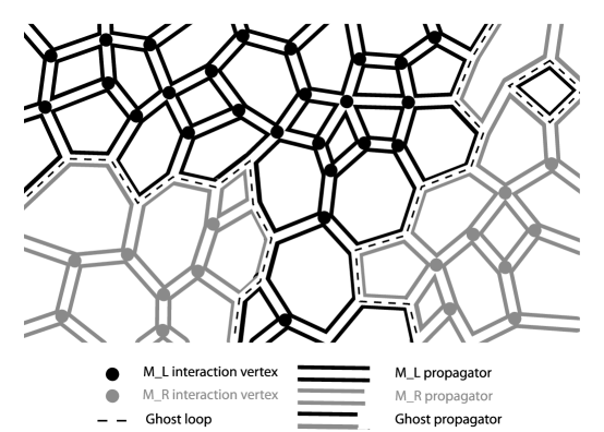
Figure 1: A Feymann diagram for the two-color $O(-2)$ matrix model (2.1).

The action (2.1) admits a good perturbative expansion. Feymann diagrams are easy to picture. Since the ghosts appear only quadratically, their propagators form self-avoiding closed loops in the Feymann diagram. There are no vertices mixing directly $\Phi_{L}$ and $\Phi_{R}$, which interact only through the coupling with the ghosts. The ghosts are $N_{L}\times N_{R}$ matrices so in the usual double-line notation each ghost loop has two sides, on one side only $\Phi_{L}$ legs are inserted, on the other only $\Phi_{R}$. Hence any Feymann graph will consist of patches of two different “colors”, $L$ or $R$, separated by the ghost loops (see Figure 1). The dual diagrams are random surfaces with the extra degrees of freedom of a gas of self-avoiding loops. There is a constraint on configurations, as there has to be an assignation of $L$ or $R$ color to each region bounded by a loop, with different colors on the two sides of each loop. In the evaluation of the diagram, each self-avoiding loop carries a weight of $-2$ (the minus sign because of odd-Grassmanality, and the factor of two because there are two copies $i=1,2$ of the $C_{i}$, $\bar{C}_{i}$).

Loop gas models on random surfaces are well studied (e.g. [57, 77, 78, 79, 80, 81, 82, 83, 84]). In the $O(n)$ model one assigns a weight of $n$ to each self-avoiding loop. Our case is then related to the $O(-2)$ model. However the usual version of the $O(-2)$ model [57] is formulated on a random surface with only “one-color”. It is immediate to write the matrix model whose perturbative expansion generates the one-color $O(-2)$ loop gas [57],

$$\int d\Phi\,dC\,d\bar{C}\;e^{-S_{1}}\,,$$ (2.9)

where

$$\displaystyle S_{1} \equiv \frac{1}{g}\,{\rm Tr}[V(\Phi-a)-2a\bar{C}C+\bar{C}\Phi C+\Phi\bar{C}C]$$

$$= \frac{1}{g}\,{\rm Tr}[V({\cal M})+\bar{C}{\cal M}C+{\cal M}\bar{C}C]\,.$$

(Here we have defined ${\cal M}\equiv\Phi-a$.) We obtain the two-color model (2.1) from (2.1) by setting

$$\Phi=\left(\begin{array}[]{cc}\Phi_{L}&0\\ 0&\Phi_{R}\end{array}\right)\,,\quad C=\left(\begin{array}[]{cc}0&C_{1}\\ \bar{C}_{2}&0\end{array}\right)\,.$$ (2.11)

The two-color model can be thought of as a ${\bf Z}_{2}$ orbifold of the one-color model. The orbifold operation introduces a twisted sector of operators odd under $\Phi_{L}\leftrightarrow\Phi_{R}$. At genus zero the untwisted sector (operators even under $\Phi_{L}\leftrightarrow\Phi_{R}$) is isomorphic to the one-color model, since “coloring” is trivial on the sphere. At higher genus the two theories differ also in the untwisted sector, since the two-color model has an additional constraint on configurations: the number of ghost loops linked to each non-trivial homology cycle of the surface must be even.

2.2 Twist lines and RNS

A familiar way to implement an orbifold is to relax the constraint and introduce “twist lines”: On a surface of genus $g$, we pick $2g$ independent homology cycles ${\cal C}_{j}$, $j=1,\dots,2g$, and write the partition function as an average over the $2^{2g}$ sectors labeled by the choices of signs $\epsilon_{j}=\pm 1$ for each homology cycle. Introducing into the partition function the factor of $\prod_{j}\epsilon_{j}^{\#{\rm loops\;linking\;}{\cal C}_{j}}$ implements the ${\bf Z}_{2}$ orbifold. For example, for the genus one vacuum amplitude, we can write

$$Z_{g=1}=\sum_{k,l\in{\bf Z}}\frac{(1+(-1)^{k})(1+(-1)^{l})}{4}Z^{(0)}_{g=1}(k,l)=\sum_{k,l\in 2{\bf Z}}Z^{(0)}_{g=1}(k,l)\,,$$ (2.12)

where the integers $k$ and $l$ denotes the number of ghost loops homotopic to the $a$- and $b$-cycle of the torus, respectively; we also defined the amplitude $Z^{(0)}_{g=1}(k,l)$ of the matrix model without any color constraint. The sector that includes the factor $(-1)^{k}$, for example, corresponds to the torus with the twist-line along the $b$-cycle.

Matrix model operators consisting of even (odd) power of $M$ are even (odd) with respect to the symmetry $\Phi_{L}\leftrightarrow\Phi_{R}$ (see (2.8)). In the formulation where we drop the color constraint and add twist lines, the appropriate signs for odd operators are accounted for by making them end-points for twist lines. Indeed a twist line between two insertion points will give a minus sign if they lie in patches of different color, a plus if they lie in patches of the same color (see Figure 2).

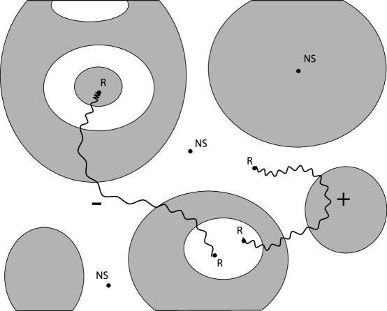
Figure 2: Twist lines and Ramond operators

In the double-scaling limit of the two-cut matrix model, the even and odd operators correspond respectively to NSNS and RR vertex operators [19]. It is then compelling to identify the $2^{2g}$ sectors described above with the $2^{2g}$ choices of spin structures in the continuum RNS formulation. For example, the torus amplitude (2.12) can be regarded as that projected by the Type 0 GSO projection

$$Z_{g=1}={\rm{Tr}}_{NSNS}\left[\frac{1+(-1)^{f_{L}+f_{R}}}{2}\right]+{\rm{Tr}}_{RR}\left[\frac{1+(-1)^{f_{L}+f_{R}}}{2}\right],$$ (2.13)

where $f_{L,R}$ is the left or right-moving world-sheet fermion number. Twist lines joining odd operators in the loop gas model clearly correspond to cuts joining spin fields on the RNS worldsheet.

This seems a step forward in understanding how the matrix model is providing a discretization of a superRiemann surface. Clearly this program is not complete, since the two-color matrix model (2.1) is building bosonic random surfaces, with some extra matter degrees of freedom in the form of ghost loops. It would be very interesting to derive (2.1) from a super-geometric formulation that includes explicitly the path integral over the gravitinos. What we have learnt so far is that the minimal Type 0B strings must have (at least perturbatively) a formulation as bosonic strings.

2.3 Relation with 0A

With some hindsight, the perturbative equivalence of the 0B theory to a bosonic string is not too surprising. The ${\bf Z}_{2}$ orbifold relating the two-color to the one-color model projects out all odd operators. In the continuum limit, this is the orbifold relating the 0B to the 0A minimal superstrings, which projects out all RR closed string vertex operators. It is known that the string equations for 0A $(2,4k)$ model are perturbatively equivalent to the string equations for the bosonic $(2,2k-1)$ models [58, 19, 29, 45]. Hence we should expect that the $(2,4k)$ 0B theory is perturbatively equivalent to a ${\bf Z}_{2}$ orbifold of the bosonic $(2,2k-1)$ model.

This circle of ideas can be completed by showing directly that the complex matrix model for the 0A theory is equivalent to the one-color loop gas. The complex matrix model reads

$$\int d{\cal M}d{\cal M}^{\dagger}e^{-\frac{1}{g}{\cal V}({\cal M}^{\dagger}{\cal M})}\,,$$ (2.14)

where ${\cal M}$ is a complex $N\times(N+q)$ matrix. Taking $q=0$, we can gauge-fix to ${\cal M}={\cal M}^{\dagger}$ hermitian and positive-definite. By a reasoning analogous to (2.2,2.3), we are led to introduce the ghosts $C$, $\bar{C}$ and to reproduce precisely the action (2.1). In deriving the one-color model by this route, the integration in (2.1) is restricted to positive-definite matrices ${\cal M}$,

$$\int_{{\cal M}\geq 0}\,d{{\cal M}}\,dC\,d\bar{C}\;\exp\left(-\frac{1}{g}\,{\rm Tr}[V({\cal M})+\bar{C}{\cal M}C+{\cal M}\bar{C}C]\right)\,,$$ (2.15)

where $V({\cal M})\equiv{\cal V}({\cal M}^{2})$. This restriction makes no difference to each order in the perturbative expansion, and corresponds to the natural non-perturbative definition of the 0A model. Let us mention for completeness the generalization to $q\neq 0$. The gauge-fixing requires the introduction of some extra fermionic variables, the $q\times N$ matrix $\bar{b}$ and the $N\times q$ matrix $b$, leading to

$$\int_{{\cal M}\geq 0}\,d{{\cal M}}\,dC\,d\bar{C}\;\,db\,d\bar{b}\;\exp\left(-\frac{1}{g}\,\left({\rm Tr}[V({\cal M})+\bar{C}{\cal M}C+{\cal M}\bar{C}C]+\bar{b}{\cal M}^{2}b\right)\right)\,.$$ (2.16)

The perturbative equivalence between the $(2,4k)$ 0A with $q=0$ and the $(2,2k-1)$ bosonic models [58, 19, 29, 45] can be readily understood by establishing a map between the respective matrix models, as we now review. Diagonalizing ${\cal M}={\rm diag}(\mu_{i})$ and integrating out the ghosts in (2.15), one has

$$\prod_{k=1}^{N}\int_{0}^{\infty}d\mu_{k}\,\prod_{i<j}(\mu_{i}-\mu_{j})^{2}\,\prod_{i,j}(\mu_{i}+\mu_{j})\,e^{-\frac{1}{g}V(\mu_{k})}\,.$$ (2.17)

The change of variables $h_{i}=\mu_{i}^{2}$ gives

$$\prod_{k=1}^{N}\int_{0}^{\infty}dh_{k}\,\prod_{i<j}(h_{i}-h_{j})^{2}\,e^{-\frac{1}{g}V(\sqrt{h_{k}})}=\int_{H\geq 0}dH\,e^{-\frac{1}{g}V(\sqrt{H})}\,.$$ (2.18)

This is almost the same as the hermitian one-matrix model for the matrix $H\equiv{\cal M}^{2}$, with the differences that 1)For generic potentials $V({\cal M})$, the action contains square roots of $H$; 2)The integration runs only over positive eigenvalues of $H$. However, for our purposes, we are only interested in even polynomial potentials $V({\cal M})$, which are polynomials in $H$. This is obvious from the point of view of the 0A model, since $V(\sqrt{H})={\cal V}(H)$. Following the route from the 0B theory, in going from the two-color to the one-color model we are restricting by definition to the “untwisted” sector of operators even under $\Phi_{L}\leftrightarrow\Phi_{R}$, which map to even powers of ${\cal M}$, ${\rm Tr}{\cal M}^{2n}={\rm Tr}H^{n}$. Moreover, the difference in the integration region has only effects which are non-perturbative in $1/N$, and is thus immaterial to all orders in the genus expansion. Thus the one-color model is (perturbatively) equivalent to the standard one-matrix model. Its multicritical points correspond in the continuum limit to the $(2,2k-1)$ Virasoro minimal models coupled to Liouville, as anticipated.

3 Loop gas models for pure supergravity

We now elaborate on the simplest example. The $(2,4)$ 0B theory ($\hat{c}=0$) is obtained from the two-cut matrix model with a quartic potential $V(M)=\frac{1}{4}(M^{2}-a^{2})^{2}$ [19]. In the large $N$ limit, for $\mu>0$ one considers a two-cut ansatz for the eigenvalues. The critical point is reached when the two cuts meet at the origin with a zero of the resolvant $R(z)$. In our normalizations, this happens for $gN\to\frac{a^{4}}{4}$ from below. The double-scaling limit consists in setting $gN=\frac{a^{4}}{4}-\epsilon\,\mu$, $\epsilon\to 0$, where $\mu$ is the bulk cosmological constant, and zooming in around the origin of the $z$ plane, $z=\epsilon\,x$.

In the loop gas model (either in the two-color or one-color version), this critical point corresponds to the so-called “dilute phase”. The loop degrees of freedom are becoming massless as we approach the critical point (the effective mass for the ghosts is the distance of the eigenvalue cut from the origin), so that the number of vertices occupied by the ghosts is diverging. Simultaneously the potential $V$ is also becoming critical, which causes the number of unoccupied vertices to also diverge. (By contrast, the dense phase would correspond to the ghost degrees of freedom filling the random surface in the continuum limit.) In fact, this particular choice of quartic potential corresponds to a higher multicritical point, where both cubic and quartic vertices are diverging [79]. Standard formulas for the $O(n)$ model (see e.g. [84]) give the the central charge of the matter and Liouville continuum CFT,

$$n=-2\cos\left(\frac{\pi}{b^{2}}\right)\,,\quad Q=b+\frac{1}{b}\,,\quad c_{L}=1+6Q^{2}=26-c_{M}\,,$$ (3.1)

where $b<1$ ($b>1$) in the dilute (dense) phase. In our case we have $n=-2$ in the dilute phase, and the multicritical quartic potential corresponds to $b=1/\sqrt{2}$, $c_{M}=-2$, $c_{L}=28$, which are indeed the values expected for the minimal $(1,2)$ bosonic string theory. Notice that we are landing on theory with $b=1/\sqrt{2}$ rather than $b=\sqrt{2}$, so we are accurately referring to this theory as the $(p,q)=(1,2)$ model (as opposed to $(2,1)$), in conventions where $b^{2}=p/q$. This subtlety is immaterial for the closed string sector, which is our focus in this section, but plays a role for D-branes, as we shall see in section 5.

Following (2.17,2.18), the one-color loop gas model with quartic potential $V({\cal M})$ can be mapped to a one-matrix integral with a gaussian potential,

$$\int_{H\geq 0}dH\,e^{-\frac{1}{4g}(H-a^{2})^{2}}\,.$$ (3.2)

In this model, the large $N$ eigenvalue density is the usual Wigner distribution, supported in the interval $[\frac{a^{2}}{2}-(gN)^{\frac{1}{2}},\frac{a^{2}}{2}+(gN)^{\frac{1}{2}}]$. As $gN\to\frac{a^{4}}{4}$, the left boundary of the cut reaches the origin (which is also the boundary of the integration region in (3.2)). The double-scaling limit is again obtained by zooming in around the origin. The double-scaling limit of the gaussian model is well-known to yield the $(2,1)$ minimal bosonic string [2, 63], which is equivalent to topological gravity [85, 86, 87, 88], see [44] for a recent simple derivation. Our model is not quite the usual gaussian model in that we have a restriction of the integration region to positive $H$ eigenvalues. We can think of having an infinite potential wall at $H=0$ that prevents eigenvalues to explore the region with $H<0$. In the doubled-scaled variables, the wall is a finite distance away in units of $\mu$ and its effects are non-perturbative in $g_{s}$.

3.1 The supersymmetric matrix model

The case of quartic potential $V$ is especially interesting since we can view the one-color model (2.1) as a matrix model with Parisi-Sourlas supersymmetry. Introducing the matrix superfield

$${\bf\Phi}(\theta,\bar{\theta})=\Phi+\bar{\theta}C+\theta\bar{C}+\theta\bar{\theta}F\,,$$ (3.3)

we can rewrite action $S_{1}$ in superspace [60, 61],

$$S_{1}=\frac{1}{g}\,\int d\theta d\bar{\theta}\;{\rm Tr}(\partial_{\theta}{\bf\Phi}\partial_{\bar{\theta}}{\bf\Phi}+{\cal W}({\bf\Phi}))\,,\quad{\cal W}({\bf\Phi})=-a{\bf\Phi}^{2}+\frac{1}{3}{\bf\Phi}^{3}\,.$$ (3.4)

In fact, this supersymmetric model is equivalent to the gaussian model (3.2) for any choice of superpotential ${\cal W}(\bf\Phi)$, by the “Nicolai map” $H={\cal W}^{\prime}(\Phi)+a^{2}$ [61]. This formulation has also an immediate interpretation as a theory of matrix fields living in minus two dimensions [59, 60, 61]. The perturbative expansion in superspace realizes the discretization of a Riemann surface embedded in minus two dimensions, which of course agrees with the value $c_{M}=-2$ of the continuum string theory. The Feynman diagrams in superspace have a $\int d\theta_{j}d\bar{\theta}_{j}$ integral at vertex $j$ and a propagator $1/a^{2}-(\theta_{j}-\theta_{k})(\bar{\theta}_{j}-\bar{\theta}_{k})/a$. The propagators can be collected in an exponential like

$$e^{-a\sum_{(jk)}(\theta_{j}-\theta_{k})(\bar{\theta}_{j}-\bar{\theta}_{k})}$$ (3.5)

This is the discretization of the continuum CFT of two free Grassmann odd scalars, with action

$$\frac{1}{4\pi}\int d^{2}z\,\epsilon_{\alpha\beta}\partial\Theta^{\alpha}\bar{\partial}\Theta^{\beta}\,,$$ (3.6)

where $\alpha=\pm$. The superspace coordinates correspond to the zero modes of the $\Theta^{\alpha}$ fields, $\theta=\theta_{0}^{+}$, $\bar{\theta}=\theta_{0}^{-}$. We refer to the appendix for more details on this CFT, which plays an important role in the following.

We can now describe the continuum version of the ${\bf Z_{2}}$ orbifold that leads from the one-color to the two-color loop gas model. The effect of a twist line in the discretized theory is to flip the sign of the ghost propagators that cross it. This corresponds in the continuum to flipping the sign of the $\Theta^{\alpha}$ across the twist line, that is, to performing the orbifold $\Theta^{\alpha}\to-\Theta^{\alpha}$. We conclude that $(2,4)$ minimal fermionic string is equivalent to a bosonic non-critical string defined by coupling to Liouville the matter CFT with $c_{M}=-2$ obtained by the ${\bf Z}_{2}$ orbifold of the $\Theta^{\alpha}$ system.

3.2 Open string field theory

Finally we are in the position to point out a transparent open string field theory interpretation of the one- and two-color matrix models, in the same spirit as the proposal of [15, 16, 21] for the $c=1$ matrix model. Starting with the one-color model, we can regard (3.4) as the effective open string field theory on infinitely many localized D-branes of the $(1,2)$ minimal bosonic string. We consider D-branes which have ZZ boundary conditions in the Liouville direction and Neumann boundary conditions for the $\Theta^{\alpha}$ CFT. Since the coordinates $\theta,\bar{\theta}$ that represents the positions of the D-brane are fermionic, we get the supermatrix model (3.4). Incidentally, it is amusing to recover the matrix action as the action of Witten’s cubic OSFT [89] (on $N$ ZZ branes with Neumann boundary conditions for the $\Theta^{\alpha}$), gauged-fixed to Siegel gauge and truncated to the lowest modes. Expanding the open string field as

$$|\Psi\rangle=\sum_{i,j=1}^{N}\left(M_{ij}\,c_{1}|0\rangle_{ij}+C_{ij}\,\theta^{-}_{0}\,c_{1}|0\rangle_{ij}+\bar{C}_{ij}\,\theta_{0}^{+}c_{1}|0\rangle_{ij}+F_{ij}\theta^{+}_{0}\theta^{-}_{0}\,c_{1}|0\rangle_{ij}+\dots\right)\,,$$ (3.7)

one can evaluate the Witten action with the usual CFT rules [90]. The kinetic term $\langle\Psi,c_{0}L_{0}\Psi\rangle$ gives precisely the quadratic terms in (3.4), with the $\partial_{\theta}\partial_{\bar{\theta}}$ derivatives arising from the zero mode terms of $L_{0}$; while the interaction term $\langle\Psi,\Psi,\Psi\rangle$ gives the cubic term of the superpotential.

The ${\bf Z}_{2}$ projection (2.11) leading to the two-color model (2.1) can now be recognized as the usual rule [91] to perform a ${{\bf Z}_{2}}$ orbifold on the D-brane worldvolume,

$${\bf\Phi}(\theta,\bar{\theta})=\sigma_{3}\cdot{\bf\Phi}(-\theta,-\bar{\theta})\cdot\sigma_{3}\,,$$ (3.8)

where $\sigma_{3}={\rm diag}(I_{N_{L}},-I_{N_{R}})$.

4 The continuum bosonic formulation

The previous arguments show that we can view the $(2,4k)$ minimal superstrings as bosonic strings, to each order in perturbation theory. The 0A theories map to the bosonic $(2,2k-1)$ strings [19, 58, 29, 45], while the 0B theories to a ${\bf Z}_{2}$ orbifold of these models. We now analyze this correspondence in the continuum worldsheet formulation.

4.1 The operator spectrum

The first task is to establish a map between the physical vertex operators of the superstring and the physical vertex operators of the bosonic formulation. We shall see that the bosonic CFTs are not the usual $(2,2k-1)$ minimal models (at least not for the 0B cases), but extensions with an infinite number of Virasoro primaries. A complete understanding will require the specification of the precise operator content and the construction of modular invariant partition functions. Here we consider the simpler problem of listing the Virasoro representations that appear in these CFTs. Our discussion partly overlaps with [19, 29]. In this subsection we assume $k>1$ and come back to the special case $k=1$ below.

The primary operators of the $(p,q)=(2,4k)$ superminimal models are labeled in the usual Kac table notation as $(r,s)=(1,s)$, with $1\leq s\leq 2k$. Operators with odd $s$ are in NSNS sector, while operators with even $s$ are in the RR sector. The operator $(1,2k)$ is the RR ground state, while $(1,1)$ is of course the identity. In the 0A theory with $\mu>0$, only NSNS operators survive the GSO projection, while in the 0B theory with $\mu>0$ all operators are kept. To construct the physical tachyon vertex operators ${\cal T}_{rs}$ one needs to gravitationally dress the superconformal primaries with a Liouville factor $e^{\beta_{rs}\phi}$, with the exponent obeying the Seiberg bound $\beta_{rs}\leq Q/2$. It is convenient to quote the rescaled dressings $\gamma_{rs}=\beta_{rs}/Q$ (the rescaling is such that the Seiberg bound is at 1/2). For the $(2,4k)$ models,

$$\gamma_{1\,s}=\frac{s+1}{2(2k+1)}\,.$$ (4.1)

In the bosonic $(2,2k-1)$ minimal models, operators are labeled as $(\tilde{r},\tilde{s})=(1,\tilde{s})$ with $1\leq\tilde{s}\leq k-1$. Tachyon vertex operators $\tilde{\cal T}_{1\,\tilde{s}}$ have rescaled Liouville dressings (again in units where the Seiberg bound is at 1/2)

$$\tilde{\gamma}_{1\,\tilde{s}}=\frac{2\tilde{s}+2}{2(2k+1)}\,.$$ (4.2)

We shall shortly need the more general formula

$$\tilde{\gamma}_{\tilde{r}\,\tilde{s}}=\frac{2k+1-\tilde{r}(2k-1)+2\tilde{s}}{2(2k+1)}\,.$$ (4.3)

The matching between the bosonic and fermionic theories is now straightforward using KPZ scaling. KPZ scaling [92, 93] tells us that the partition function $F_{g}(\{t_{n}\})$ at genus $g$, as a function of the sources $\{t_{n}\}$ for the local operators of the theory, is a homogeneous function of degree $Q(1-g)$, where each $t_{n}$ is assigned the weight $\gamma_{n}$ equal to its rescaled Liouville (or superLiouville) dressing. Comparison of (4.1) and (4.2) leads to $s=2\tilde{s}+1$, i.e. to the identification

$${\cal T}_{1\,2\tilde{s}+1}\cong\tilde{\cal T}_{1\,\tilde{s}}\,.$$ (4.4)

As expected, the bosonic vertex operators map to NSNS vertex operators in the superstring. Notice that the operator ${\cal T}_{11}$, which corresponds to the cosmological constant deformation of superLiouville theory, is absent in the minimal bosonic theory. It maps in the bosonic theory to $(1,\tilde{s}=0)$, which is just outside the minimal Kac table. This is not surprising, since this operator is associated with a redundant deformation in the KdV hierarchy – which to each order in perturbation theory governs the 0A theory as well. There are $(k-1)$ independent deformations in the integrable hierarchy, and $k$ NSNS operators in the superstring; the $k$-th operator (the one with lowest superLiouville dressing) must be redundant. In the bosonic theory this operator has a Liouville dressing equal to one half the Liouville dressing of the bulk cosmological constant (which has $\tilde{s}=1$, of course) and it can be interpreted as a “boundary operator” [94]. In modern language, it corresponds to the boundary cosmological constant operator, which can be inserted on boundaries with FZZT boundary conditions.

For the 0A theory this is the end of the story. For the 0B theory, we need to find the counterpart of the RR operators on the bosonic side. Inspection of (4.1) and (4.3) leads to match the superconformal labels $(1,s)$ for $s$ even with the bosonic labels $(\tilde{r}=2,\tilde{s})$ with $s=2(\tilde{s}-k+1)$, i.e. to the identification

$${\cal T}_{1\,2(\tilde{s}+1-k)}\cong\tilde{\cal T}_{2\,\tilde{s}}\,,$$ (4.5)

with $k\leq\tilde{s}\leq 2k-1$. Clearly all of these operators are outside the minimal bosonic Kac table. Closure of the fusion rules will generically require to include all degenerate Virasoro representations $(2,\tilde{s})$ and $(1,\tilde{s})$ with no restrictions on $\tilde{s}$. In the 0B case the enlargement of the Kac table is inevitable, and this suggests it may be natural to treat the 0A case using a non-minimal table as well (see [95] for some relevant discussions). One can check that the bosonic fusion rules are compatible with the expected ${\bf Z}_{2}$ symmetry, with the operators $(\tilde{r},\tilde{s})$ being even for $\tilde{r}=1$ and odd for $\tilde{r}=2$. It would be interesting to construct modular invariant partition functions for these non-minimal conformal field theories.

4.2 ${\bf\hat{c}=0}$ from ${\bf c=-2}$

The case of the bosonic $(2,1)$ model (more accurately $(1,2)$), for which $c_{M}=-2$, requires a separate treatment. This theory has been extensively studied [66, 67, 68, 69, 70, 71, 72, 73] as the simplest example of a logarithmic CFT. There is a free field representation of the model in terms of a pair of Grassmann odd scalars $\Theta^{+}(z,\bar{z})$ and $\Theta^{-}(z,\bar{z})$. Modular invariant partition functions have been constructed, for various choices of operator content corresponding to various orbifolds of the $\Theta^{\alpha}$ fields. Although these partition functions contain an infinite number of Virasoro primaries, they are rational with respect to a $W$-algebra. It is conceivable that a similar story could be worked out for the other $(2,2k-1)$ models. In the appendix we collect some useful formulas pertaining to the $\Theta^{\alpha}$ system.

The bosonic theory corresponding perturbatively to the $(2,4)$ 0A model can be defined taking as matter CFT simply the free $\Theta^{\alpha}$ system with periodic boundary conditions. The natural tachyon vertex operators are [34]

$${\cal O}_{n}=e^{\frac{3-n}{\sqrt{2}}\phi}{\cal P}_{n}(\partial\Theta^{\alpha},\bar{\partial}\Theta^{\beta})\,c\bar{c}\,,\quad n=1,3,5,\dots$$ (4.6)

Here $\phi$ is the Liouville field and $c$, $\bar{c}$ the usual reparametrization ghosts of the bosonic string, and ${\cal P}_{n}$ are matter primaries of dimension $(n^{2}-1)/8$ built acting on the vacuum with $\Theta^{\alpha}$ oscillator. In the notation of the previous section, these primaries correspond to the $(1,\tilde{s})$ Virasoro representations, with $\tilde{s}=(1-n)/2$. The primary ${\cal P}_{n=1}$ is just the identity, its Kac label being $(1,0)\equiv(1,1)$ by the usual reflection property $(\tilde{r},\tilde{s})\equiv(p-\tilde{r},q-\tilde{s})$. ${\cal O}_{1}$ is thus the bulk cosmological constant operator, and it maps to the only tachyon operator of the 0A $(2,4)$ model, namely the cosmological constant operator of the superLiouville theory ($s=1$ in the notations of the previous section). In this case the cosmological constant deformations of the fermionic and bosonic string theories are in correspondence with each other: the “conformal” background of the bosonic $(1,2)$ model maps to “superconformal” background of the $(2,4)$ model. This is not the case for the models with $k>1$.

For $n>1$, the operators (4.6) are interpreted as “gravitational descendants” in the topological gravity language. From the viewpoint of the bosonic string theory, they are standard elements of the cohomology at ghost number $(1,1)$. Gravitational descendants are often represented as elements of the cohomology at non-standard ghost numbers [98], in fact this is necessarily the case if the matter CFT is truly minimal. In our case, the matter CFT has infinitely many primaries and we gain the ability to represent gravitational descendants as standard vertex operators of ghost number $(1,1)$, which is perhaps a more convenient picture for actual calculations. This phenomenon is not new and has been discussed in the topological string theory literature in related contexts, see for example [99, 100, 101].

The theory corresponding to the $(2,4)$ 0B model is obtained by the ${\bf Z}_{2}$ orbifold $\Theta_{\alpha}\to-\Theta_{\alpha}$. The orbifold introduces a twisted sector built with $\Theta^{\alpha}$ oscillators acting on a vacuum of dimension $-1/8$. We refer to the appendix for the expression of the torus partition function. The twisted sector can be decomposed in irreducible Virasoro representations of dimensions $(n^{2}-1)/8$, where now $n$ is even. All these Virasoro representations are also degenerate and correspond to the $(0,\tilde{s})$ elements of the Kac table, with $\tilde{s}=-n/2$. Tachyon vertex operators are obtained by dressing with the same Liouville exponential as in (4.6), with $n$ even. The tachyon with $n=0$ maps to the RR ground state of the $(2,4)$ model. Tachyons with $n>0$ are again interpreted as gravitational descendants.

4.3 The torus path-integral

As a check of our proposal, we can evaluate the torus partition function in the continuum bosonic formulation of the $(2,4)$ model and compare it with the matrix model result. The partition function in the continuum fermionic formulation of the $(2,4k)$ models has not yet been fully computed, because the odd spin structures are somewhat subtle. The results for the even spin structures are available [102], and they match with the matrix model results [19]. For the 0A theory with $\mu>0$, the spectrum has only NSNS operators, the torus partition function coincides with that of the bosonic $(2,2k-1)$ theory, and we do not have anything new to add to the discussion in [19]. For the $(2,4)$ 0B theory with $\mu>0$ we should be able to compute the full torus partition function using our identification with the ${\bf Z}_{2}$ orbifold of the $(1,2)$ model. The expected matrix model result is (for general $k$ and $\mu>0$)

$$Z_{2,4k}^{0B}=-\frac{2k+1}{24k}\,\log t\,,$$ (4.7)

where $t$ is the coupling of the operator of lowest dimension in the theory.

This calculation is straightforward using the results of [102]. These authors computed the string theory torus path integral in the continuum formulation; in the case that the matter CFT is a boson at radius $R$ they found

$$Z^{c=1}(R/\sqrt{\alpha^{\prime}})=-\frac{1}{24}\left(\frac{R}{\sqrt{\alpha^{\prime}}}+\frac{\sqrt{\alpha^{\prime}}}{R}\right)\log t\,.$$ (4.8)

As reviewed in the appendix, the ${\bf Z}_{2}$ orbifold of the $\Theta^{\alpha}$ system has a partition function identical to a compact boson of radius $R=\sqrt{2\alpha^{\prime}}$. Thus the calculation of the torus path integral is almost identical to the one that leads to (4.8) with $R=\sqrt{2\alpha^{\prime}}$. The only difference is in the integral over the Liouville zero mode, which contributes the factor of $-\log{t}/{\beta}$, where $\beta$ is the Liouville dressing of the most relevant matter operator. The torus path integral $Z_{{\bf Z}_{2}}$ of the ${\bf Z}_{2}$ orbifold of the $(1,2)$ model can then be deduced from (4.8) if we account for the different values of $\beta$. The most relevant operator of the $(1,2)$ theory is the cosmological constant, which in our normalizations has $\beta_{c=-2}=\sqrt{2}$; the most relevant operator for $c=1$ is again the cosmological constant, which has $\beta_{c=1}=2$. Hence

$$Z_{{\bf Z}_{2}}=\frac{\beta_{c=1}}{\beta_{c=-2}}\,Z^{c=1}(\sqrt{2})=-\frac{1}{8}\,\log t\,.$$ (4.9)

This agrees with the matrix model result (4.7) for $Z^{0B}_{2,4}$.

5 D-branes

A very interesting comparison involves the realization of open string boundary conditions in the loop gas model (and its continuum limit) versus the continuum fermionic formalism. The spectrum of FZZT branes in the continuum fermionic formulation 0A and 0B theories has been determined in [32]. Let us recall their results. In the $(2,4)$ 0B theory with $\mu>0$, there are three relevant FZZT boundary states [10, 11, 14], labeled as [32]

$$|x;\eta=+1\rangle_{B}\,,\qquad|x;\eta=-1\,,\xi=\pm 1\rangle_{B}\,.$$ (5.1)

Here $x$ is the boundary cosmological constant, which takes values in the auxiliary Riemann surfaces ${\cal M}_{2,4}^{\eta=\pm}$ introduced in [32]. The label $\eta=\pm 1$ distinguishes the linear combination of left and right moving supercharges annihilating the boundary state (“electric” versus “magnetic” branes) while $\xi=\pm 1$ distinguishes a brane from its anti-brane. The $|x;\eta=+1\rangle$ brane does not couple to the RR ground state and it is thus identical to its own anti-brane. Moreover, computations of one-point functions indicate that in BRST cohomology one can identify $|x;\eta=-1;\xi\rangle=|-x;\eta=-1;=\xi\rangle$, and parametrize the independent $\eta=-1$ branes just by their value of $x$, forgetting the label $\xi$. Finally from the annulus amplitude, one finds that the open strings between branes with the same $\eta$ are in the NS sector, while open strings between branes with opposite $\eta$ are in the Ramond sector. Results for the higher $(2,4k)$ 0B models with $\mu>0$ are similar. A priori the boundary states would acquire labels corresponding to the matter primaries, however it is believed [32] (in analogy with the bosonic string) that in the BRST cohomology such labels are redundant and one can still parametrize the inequivalent boundary states by $\eta=\pm 1$, $\xi=\pm 1$ and $x$ taking value in the appropriate Riemann surface ${\cal M}^{\eta=\pm}_{(2,4k)}$.

On the other hand, in the $(2,4)$ 0A theory with $\mu>0$, the relevant boundary states are

$$|x;\eta=+1\,,\xi=\pm 1\rangle_{A}\,,\qquad|x;\eta=-1\,\rangle_{A}\,.$$ (5.2)

In the 0A theory with $\mu>0$ the RR ground state does not give rise to a local vertex operator [19], but it corresponds to the zero mode of the RR field, under which the $\eta=+1$ brane is charged; changing the sign of $\xi$ reverses the charge of the brane.

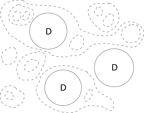
Figure 3: Dirichlet boundary conditions for $\Theta^{\alpha}$ in the loop gas model. The dashed lines represent the self-avoiding ghost loops.

5.1 The ${\bf\eta=-1}$ brane

For both 0A and 0B, the FZZT branes with $\eta=-1$ have been identified [19, 32] with the standard macroscopic loop operators of the corresponding matrix model.

5.1.1 0A

Let us consider the 0A case first. The loop operator is

$$W^{\eta=-1}_{A}(x_{A})=-\frac{1}{N}{\rm Tr\;log}({\cal M}^{\dagger}{\cal M}-x_{A})\to-\frac{1}{N}{\rm Tr\;log}({\cal M}^{2}-x_{A})=-\frac{1}{N}{\rm Tr\;log}(H-x_{A})\,,$$ (5.3)

where the arrow indicates the gauge-fixing procedure of section 2.3. In terms of the matrix $H$, this is the standard resolvant of the one-matrix model; perturbatively, results for the resolvant expectation values in $(2,4k)$ 0A coincide with those in $(2,2k-1)$ bosonic. However it would be wrong to attempt to match the auxiliary Riemann surfaces computed in [32] between bosonic and fermionic models. This is because the results of [32] are valid for conformal or superconformal backgrounds, but for general $k$ the cosmological constant deformation of the bosonic theory does not correspond to the cosmological constant deformation of the 0A theory. They do match for $k=1$; indeed in this case the $\eta=-1$, $\mu>0$ curve for 0A coincides with the curve $2y^{2}-1=x$ [32] of the $(2,1)$ bosonic theory (up to rescalings of $x$ and $y$).

It is clear that in our formulation in terms of the one-color loop gas, $W^{\eta=-1}_{A}(x)$ cuts a macroscopic hole which cannot intersect any of the self-avoiding ghost loops, since the matrices $C_{i}$ do not appear in $W^{\eta=-1}_{A}$ (see Figure 3). Let us now focus on the $k=1$ case. In the supersymmetric formalism of section 3.1, we can write

$$W^{\eta=-1}_{A}(x_{A})=-\frac{1}{N}{\rm Tr\;log}(({\bf\Phi}-a)^{2}-x_{A})|_{\theta=\bar{\theta}=0}\,.$$ (5.4)

In the continuum limit, this operator cuts a hole in the worldsheet with Dirichlet boundary conditions $\Theta^{\alpha}=0$ for the $c_{M}=-2$ CFT. Notice however that in the supersymmetric model, the more natural expression for the resolvant is

$$W_{(1,2)}(x)=-\frac{1}{N}{\rm Tr\;log}(({\bf\Phi}-a-x)|_{\theta=\bar{\theta}=0}\,.$$ (5.5)

In the double-scaling limit, $W_{(1,2)}$ and $W^{\eta=-1}_{A}(x_{A})$ are equivalent with $x_{A}$ scaling as $x^{2}$. This relation between $x$ and $x_{A}$ reflects the fact that the continuum limit of the one-color gas model gives what should be more accurately referred to as the $(p,q)=(1,2)$ minimal bosonic string, the one with $b\equiv\sqrt{p/q}=1/\sqrt{2}$; while the continuum limit of the gaussian model gives the $(2,1)$ theory with $b=\sqrt{2}$. There is no distinction between $(1,2)$ and $(2,1)$ in the closed string sector but open string boundary conditions are labeled differently. The boundary cosmological $\mu_{B}$ constant of the $(1,2)$ model is equal to the dual boundary cosmological $\tilde{\mu}_{B}$ of the $(2,1)$ model, and vice-versa. Now $\mu^{(2,1)}_{B}\equiv\tilde{\mu}^{(12)}_{B}=2(\mu^{(1,2)}_{B})^{2}-\mu$, which is compatible with the identifications $x_{A}\sim\mu_{B}^{(2,1)}$ and $x\sim\mu_{B}^{(1,2)}$. FZZT branes with Dirichlet boundary conditions for $\Theta^{\alpha}$ in the $(1,2)$ have been considered in [34], where is is shown that the full cubic OSFT on them localizes to the Kontsevich model. The authors of [44] reproduced this result starting with the resolvant (5.3) for the gaussian matrix model in terms of the matrix $H$, and performing the double-scaling limit; they observed that in their procedure one lands to the $(2,1)$ model with $b=\sqrt{2}$, a fact that we have just explained from the relation between the gaussian and loop-gas matrix models.

More generally the full superfield loop operator,

$$W_{(1,2)}(x,\rho^{\alpha})=-\frac{1}{N}{\rm Tr\;log}(({\bf\Phi}-a-x)|_{\theta=\rho,\bar{\theta}=\bar{\rho}}\,,$$ (5.6)

gives in the continuum limit the FZZT brane tensored with the Dirichlet boundary state $|{\rm Dir}(\rho^{\alpha})\rangle$ for the $\Theta^{\alpha}$ system (see (A.13) in the appendix).

5.1.2 0B

Let us now consider the $\eta=-1$ brane for the 0B model. This is naturally identified with the macroscopic loop operator of the two-cut matrix model,

$$\displaystyle W^{\eta=-1}_{B}(x_{B}) = -\frac{1}{N}{\rm Tr\;log}(M-x_{B})=-\frac{1}{N}{\rm Tr\;log}(-x_{B}-a+\Phi_{L})-\frac{1}{N}{\rm Tr\;log}(-x_{B}+a-\Phi_{R})$$ (5.7)

$$= \frac{1}{N}\,\sum_{l}\frac{{\rm Tr}\,\Phi_{L}^{l}}{l\,(a+x_{B})^{l}}+\frac{1}{N}\,\sum_{l}\frac{{\rm Tr}\,\Phi_{R}^{l}}{l\,(a-x_{B})^{l}}-\frac{1}{N}\log(x_{B}^{2}-a^{2})\,.$$

Again in the two-color loop gas model the ghost loops do not intersect the boundary (Figure 3). It is also clear from (5.7) that the expansion of $W^{\eta=-1}_{B}(x_{B})$ contains both even and odd operators under $\Phi_{L}\leftrightarrow\Phi_{R}$, which in the continuum limit are identified as NSNS and RR operators. This is just as expected for the $\eta=-1$ branes, which couple both to NSNS and RR closed operators (see (5.1)). We can be more precise. In the expansion of $W^{\eta=-1}_{B}(x_{B})$, we weight a boundary of length $l$ differently according to its color, either with a factor proportional to $1/(a+x)^{l}$ for the color $L$ or with a factor proportional to $1/(a-x)^{l}$ for the color $R$. To express this fact in the formalism of the unconstrained loop gas with twist lines, we must extend to sum to new sectors, allowing for twist lines that end on a boundary. The weight for a boundary of length $l$ must be taken

$$\frac{1}{l\,(x_{B}+a)^{l}}+\frac{\epsilon}{l\,(x_{B}-a)^{l}}$$ (5.8)

where $\epsilon=+1$ in the sector where no twist line ends on the boundary and $\epsilon=-1$ if it does. This fits perfectly with the continuum RNS formulation, where the $\eta=-1$ branes have both an RR and an NSNS term in their boundary state and thus one must sum over the different sectors in the closed channel. If we remove the distinction between $L$ and $R$ (that is, project out the odd operators),

$$W^{\eta=-1}_{B}(x_{B})\longrightarrow-\frac{1}{N}{\rm Tr\;log}((\Phi-a)^{2}-x_{B}^{2})=W^{\eta=-1}_{A}(x_{A}=x_{B}^{2})\,.$$ (5.9)

The relation $x_{A}=x_{B}^{2}$ is as expected [19, 32].

We can now analyze the 0B $\eta=-1$ brane in the continuum bosonic formulation. The boundary state is obtained by taking the ${\bf Z}_{2}$ orbifold of the FZZT brane with Dirichlet boundary conditions $\Theta^{\alpha}=0$. The orbifold operation yields two fractional branes with opposite coupling to the twisted sector, which we identify with the $|\eta=-1,\xi=\pm 1\rangle_{B}$ branes. This clearly agrees with the discretized expression (5.7), which cuts holes in the worldsheet with Dirichlet b.c. for the $\Theta^{\alpha}$, and on which twist lines can end.

5.2 The ${\bf\eta=+1}$ brane

The brane with $\eta=+1$ has so far been more puzzling, since it does not appear to correspond to standard macroscopic loop operators in the one- or two-matrix models [19, 32]. In our formalism (focussing on the $(2,4)$ case) there is a natural guess for what this brane should correspond to, namely the other natural choice of boundary conditions in the $\Theta^{\alpha}$ system: Neumann boundary conditions. The most compelling piece of evidence for this proposal comes from consideration of the open string spectrum between Neumann and Dirichlet branes for the $\Theta^{\alpha}$ system, which lies in the twisted sector (see (A.16)) – and hence has “half-integer” Liouville dressing (i.e. $n$ even in the notations of section 4.2). This agrees with the fact that the open strings between $\eta=-1$ and $\eta=+1$ branes are in the Ramond sector. Since the identification of the $\eta=-1$ brane with Dirichlet b.c. for $\Theta^{\alpha}$ is beyond any doubt, we seem to be forced to identify the $\eta=+1$ brane with Neumann b.c. for $\Theta^{\alpha}$ in order to reproduce the correct open string spectrum.

In the matrix model, we can find an expression for the Neumann macroscopic loop operator by appealing to the string theory intuition. We regard the matrix model as the open string field theory on Neumann ZZ branes as in [15, 16]. To a Neumann FZZT brane we add the open strings stretched between the Neumann FZZT brane and the $N$ Neumann ZZ branes. Such open strings are expected to be fermionic [44], and since we have $\Theta^{\alpha}$ Neumann b.c. on both branes, they will depend on the $\Theta^{\alpha}$ zero modes. Thus we need to introduce a Grassmann odd open string field $\pi(\theta,\bar{\theta})$ in the fundamental of $U(N)$. In the supersymmetric formulation we think of it as a new superfield. We are led to the matrix model

$$\int d{\bf\Phi}\,d\pi\;e^{-(S_{\bf\Phi}+S_{\pi})}$$ (5.10)

with

$$S_{\bf\Phi}=\int d\theta d\bar{\theta}\;{\rm Tr}(\partial_{\theta}{\bf\Phi}\partial_{\bar{\theta}}{\bf\Phi}-a{\bf\Phi}^{2}+{\bf\Phi}^{3})\,,\quad S_{\pi}=\int d\theta d\bar{\theta}\;(\partial_{\theta}{\bf\pi}^{\dagger}\partial_{\bar{\theta}}{\bf\pi}+w{\bf\pi}^{\dagger}{\bf\pi}+{\bf\pi}^{\dagger}{\bf\Phi}{\bf\pi})\,,$$ (5.11)

where $w$ is a mass parameter. In the Feynman diagram expansion, the new field introduces boundaries which are free to fluctuate in the $\Theta^{\alpha}$ directions. In the loop gas picture, now there will be ghost lines attaching to the boundary. The $\pi$ superfield can be integrated out,

$$\int d{\bf\Phi}\cdot\det(\Phi+w)^{-2}\cdot\det\left((\Phi+w)^{2}-\bar{C}\frac{1}{\Phi+w}C-F\right)\cdot e^{-S_{\bf\Phi}}.$$ (5.12)

One can imagine to further integrate out $F$, $C$ and $\bar{C}$. This would lead to a complicated expression involving a sum of multitrace combinations of the lowest-component matrix $\Phi$. We leave a detailed study of this new resolvant and of its double-scaling limit for future work.

It would be nice to understand in the framework of the continuum bosonic formulation why Neumann brane for $\Theta^{\alpha}$ should be a source of RR charge in the 0A model, but not in the 0B model (see (5.1, 5.2)). At present we have no crisp answer. RR charge is related to the very subtle RR ground state, which both in the supersymmetric and in the bosonic formulations precisely saturates the Seiberg bound. A logical possibility is that while minimal superstrings are perturbatively equivalent to bosonic strings in the closed string sector, this equivalence breaks down for D-branes, which are non-perturbative objects. This is a valid objection for ZZ branes. In the matrix model ZZ branes are related to stationary points of the effective eigenvalue potential, and the non-perturbative restriction on the range of eigenvalue integration will affect their spectrum. However, we expect that FZZT branes should have a good description in the bosonic formulation. Intuitively this is because FZZT branes can be continuously connected to the closed string vacuum by sending the boundary cosmological constant to infinity, and in that limit they admit an expansion in closed string operators. We hope that a better understanding of the matrix model (5.11) and of its continuum limit will clarify this issue.

5.3 Comparison with previous work

We would like to make contact with previous discussions of boundary conditions for loop gas models [82, 83, 84]. Loop gas models can be formulated as “height” models (see [84] for a recent discussion), where configurations are specified by assigning a height variable to each vertex of a triangulated random surface (the heights of two neighboring vertices differing at most by one unit). The self-avoiding loops are the domain walls separating regions of the surface of different heights. The height model of [84] is rich enough to describe the (dicretized version of) non-minimal matter of central charge $c_{M}\leq 1$ plus Liouville CFT of central charge $c_{L}=26-c_{M}$. In the continuum limit, the height variable of [84] goes over an anomalous free boson $X$ which provides a Coulomb gas representation of the matter CFT. In the height model, the natural boundary conditions are “Dirichlet” (fixed height at the boundary) and “Neumann” (free sum over different heights at the boundary). “Dirichlet” boundary conditions are equivalent to not allowing the self-avoiding loops to touch the boundary. In the continuum limit, they correspond to Dirichlet boundary conditions for the matter field $X$, and FZZT boundary conditions for the Liouville BCFT. The “Neumann” boundary conditions of [82, 83, 84] correspond instead to summing over all possible configurations, with self-avoiding loops allowed to end on the boundary. In the continuum limit, these boundary conditions go over Neumann boundary conditions for the Coulomb gas field $X$, and dual FZZT boundary conditions for the Liouville [84]. Dual FZZT boundary conditions mean that the dual deformation $e^{\phi/b}$ is turned on the worldsheet boundary as opposed to $e^{b\phi}$. In fact, we know from the FZZT boundary CFT [10] that both the $e^{b\phi}$ and $e^{\phi/b}$ deformations are actually turned on in the exact solution, so in the Liouville sector the distinction between ordinary and dual FZZT b.c. is immaterial (up to relabeling parameters); however in the matter sector, the distinction between “Neumann” and “Dirichlet” b.c. for $X$ is significant.

The boundary conditions that we have identified with the $\eta=-1$ FZZT brane, namely Dirichlet boundary conditions for $\Theta^{\alpha}$, are clearly the same as the “Dirichlet” boundary conditions of [84]. However it is not at all obvious that Neumann boundary conditions for the $\Theta^{\alpha}$ system (and their discretized version (5.11)) are the same as the “Neumann” boundary conditions of [84]. The continuum limit of the height model of [84] (specializing their formulas to $n=-2$ in the dilute phase) gives a free anomalous boson $X$ with $c_{M}=-2$ coupled to Liouville. Clearly “Neumann” boundary conditions for $X$ have nothing to do with Neumann boundary conditions for $\Theta^{\alpha}$. However this comparison with the formulas of [84] is naive, because their model is different from ours in some crucial ways, even in the one-color case. The supersymmetric matrix model corresponds to a $O(-2)$ loop gas model with multicritical quartic potential [79]; whereas the model of [84] is based on a triangulation of the surface. Another (probably related) point is that the $\Theta^{\alpha}$ CFT does not need screening charges, whereas the $X$ CFT does. It will be very interesting to extend the formalism of [84] to our case. It is conceivable that a suitable modification of the loop equation approach of [82, 84] to “Neumann” boundary conditions may turn out to be equivalent to (5.11), and provide a way to do concrete calculations.

6 Outlook

We have seen that the matrix models of minimal superstrings have a very natural formulation as loop gas models on random surfaces. This language has many virtues.

First, it clarifies the ${\bf Z}_{2}$ orbifold relation between the 0A and 0B matrix models, which amounts to going from an ordinary random surface to a bicolored random surface. Second, it gives in the continuum limit a formulation of minimal superstrings as bosonic string theories, to each order in the perturbative expansion. The main news here are for the 0B cases, since the 0A cases have no local RR operators in the closed string spectrum and have been known to be perturbatively equivalent to minimal bosonic theories [19, 58, 29, 45]. In the 0B examples, RR operators are in the twisted sector of the ${\bf Z}_{2}$ orbifold and we have seen very explicitly how the loop gas model implements the sum over spin structures; in the simplest case of $\hat{c}=0$ this is the sum over spin structures of the $\Theta^{\alpha}$ system. One of the most intriguing directions for future work is to see if one can recover the loop gas model from a direct discretization of the RNS worldsheet. The $\Theta^{\alpha}$ fields seem vaguely reminiscent of gravitinos, in that RR operators make them multi-valued – but they have, of course, the wrong spin.

Finally, and this may turn out to be the most practical aspect of our work, loop gas models appear to give a more transparent description of open string boundary conditions. We find it very plausible that the $\eta=+1$ branes, which are mysterious in other formulations, correspond to Neumann boundary conditions for the $\Theta^{\alpha}$ system. Further work is needed to completely settle this issue. A promising direction is a detailed study the new macroscopic loop operator that we have proposed in section 5.2.

Several extensions of the results of this paper can be contemplated. More general $(p,q)$ minimal superstrings should be described by two-matrix models, and their gauge-fixing should lead to loop gas models. It would also be nice to see if a similar gauge-fixing procedure as described in this paper can give some insight into $\hat{c}=1$ string theory. Some progress in connecting the $\hat{c}=1$ Type 0A theory with the RNS formulation has been made in the interesting paper [38], and it would be nice to understand the relation between their approach and ours.

The theme that underlies the whole subject is open/closed duality. The doubled scaled matrix models dual to non-critical strings are interpreted as the effective open string field theories on a large number of decayed ZZ branes. In this paper we have seen a new sharp application of this idea. The one- and two-color loop gas models are recognized as the effective worldvolume theories on the appropriate ZZ branes; it is satisfying to see that the ${\bf Z}_{2}$ orbifold relating them is the usual string theory [91]. The other class of Liouville branes, namely the FZZT branes, offer an alternative route to open/closed duality [34], which we have not explored in this paper. The OSFT on the FZZT branes of $(1,2)$ minimal bosonic string localizes to the Kontsevich matrix model [34, 44]. The speculation of [34] is that “topological” matrix models à la Kontsevich are generically related to FZZT branes. In the context of minimal superstrings this raises many natural questions. We expect that the study of FZZT branes in minimal superstrings will lead to interesting generalizations of topological matrix models.

As usual with solvable models, the most important question is which features of the exact solution generalize to more physical situations. Open/closed duality is certainly one such feature. Other lessons specific to minimal superstrings should be sought in the study of exact RR backgrounds. In the critical RNS string, there are two related difficulties with RR backgrounds: they introduce cuts on the worldsheets and thus cannot be exponentiated in any obvious fashion; they break superconformal symmetry and thus the very rules for string theory computations are unclear. In this paper we have seen that for minimal superstrings the second difficulty can be circumvented by going to an equivalent bosonic formulation. This simplification may well be an artifact of the simplicity of these models. However, the first problem is still very much with us in the continuum bosonic formulation. Remarkably, the matrix model manages to produce an exact answer. A paradigmatic example is the Ising model with external magnetic field. Either as a continuum CFT, or as a spin system on a regular lattice, this is a notoriously difficult problem. The model becomes vastly simpler once formulated on a random lattice [103]; it can be easily mapped to a two-matrix model with asymmetric potential, and solved exactly. Summing over triangulations before summing over the spin degrees of freedom is the winning strategy. We can only speculate about the implications for critical superstrings. Perhaps the message here is that in trying to formulate RR backgrounds on a fixed Riemann surface, we are addressing a more difficult problem than we really need to solve.

Appendix A Appendix: The ${\bf\Theta^{\alpha}}$ CFT

In this appendix we review some basic facts about the “sympletic fermions” CFT [66, 67, 68, 69, 70, 71, 72, 73] and elaborate on its connections with minimal superstrings.

A.1 Bulk theory

$\Theta^{+}(z,\bar{z})$ and $\Theta^{-}(z,\bar{z})$ are non-chiral, Grassmann odd fields of dimension zero, governed by the free action

$$\frac{1}{4\pi}\int d^{2}z\,\epsilon_{\alpha\beta}\,\partial\Theta^{\alpha}\bar{\partial}\Theta^{\beta}\,.$$ (A.1)

Here $\alpha,\beta=\pm$, $\epsilon^{\pm\mp}=\pm 1$, $\epsilon_{\alpha\beta}\epsilon^{\beta\gamma}=\delta_{\alpha}^{\,\gamma}$. Hermitian conjugation acts as $(\Theta^{+})^{\dagger}=\Theta^{-}$. This CFT differs from the more familiar $\eta\xi$ system in the treatment of the zero modes. One can identify $\xi(z)+\bar{\xi}(\bar{z})=\Theta^{+}(z,\bar{z})$, $\eta(z)=\partial\Theta^{-}(z,\bar{z})$ and $\bar{\eta}(\bar{z})=\bar{\partial}\Theta^{-}(z,\bar{z})$, but there is a mismatch in the zero mode sector. While the $\eta\xi$ system has two chiral zero modes (one for the chiral field $\xi$ and one for the antichiral field $\bar{\xi}$), the $\Theta^{\alpha}$ system has two non-chiral zero modes, one for $\Theta^{+}$ and one for $\Theta^{-}$.

Let us first consider the “untwisted” theory, with periodic fields $\Theta^{\alpha}(z,\bar{z})=\Theta^{\alpha}(e^{2\pi i}z,e^{-2\pi i}\bar{z})$. The mode expansion reads

$$\Theta^{\alpha}(z,\bar{z})=\theta_{0}^{\alpha}+\chi_{0}^{\alpha}\ln|z|^{2}+i\sum_{n=-\infty\,n\neq 0}^{\infty}\left(\frac{\chi_{n}^{\alpha}}{nz^{n}}+\frac{\bar{\chi}_{n}^{\alpha}}{n\bar{z}^{n}}\right)\,.$$ (A.2)

The modes obey the obvious canonical anticommutation relations

$$\{\chi_{0}^{\alpha},\theta_{0}^{\beta}\}=\epsilon^{\alpha\beta}\,,\quad\{\chi_{m}^{\alpha},\chi_{n}^{\beta}\}=m\epsilon^{\alpha\beta}\delta_{m+n,0}\,,\quad\{\bar{\chi}_{m}^{\alpha},\bar{\chi}_{n}^{\beta}\}=m\epsilon^{\alpha\beta}\delta_{n+m,0}\,.$$ (A.3)

Notice that in correspondence with the two non-chiral zero modes $\theta_{0}^{\alpha}$, there are two canonically conjugate non-chiral momenta $\chi_{0}^{\alpha}$, i.e. one has the identification $\chi_{0}^{\alpha}\equiv\bar{\chi}_{0}^{\alpha}$, which is required by locality. The Fock space is obtained by acting with the creation operators $\chi^{\alpha}_{-n}$ and $\bar{\chi}^{\alpha}_{-n}$ $(n>0)$, on the space of ground states, which is spanned by

$$|\Omega\rangle\,,\qquad|\theta^{\alpha}\rangle\equiv\theta_{0}^{\alpha}|\Omega\rangle\,,\qquad|\omega\rangle\equiv\theta_{0}^{+}\theta_{0}^{-}|\Omega\rangle\,.$$ (A.4)

Here $|\Omega\rangle$ denotes the $SL(2,{\bf C})$ vacuum. This system provides the simplest realization of a logarithmic CFT. The states $|\Omega\rangle$ and $|\omega\rangle$ form a logaritmic pair, spanning a two dimensional Jordan block for $L_{0}$,

$$L_{0}|\omega\rangle=\bar{L}_{0}|\omega\rangle=|\Omega\rangle\,,\quad L_{0}|\Omega\rangle=\bar{L}_{0}|\Omega\rangle=0\,.$$ (A.5)

Let us also record the inner products

$$\langle\Omega|\Omega\rangle=\langle\theta^{\alpha}|\Omega\rangle=\langle\theta^{\alpha}|\omega\rangle=0\,,\quad\langle\Omega|\omega\rangle=1\,,\quad\langle\theta^{\alpha}|\theta^{\beta}\rangle=\epsilon^{\alpha\beta}\,,\quad\langle\omega|\omega\rangle=\kappa\,.$$ (A.6)

Here $\kappa$ is an arbitrary normalization constant, corresponding to the freedom to redefine $|\omega\rangle\to|\omega\rangle+\alpha|\Omega\rangle$. If we stick to the definition in (A.4), then $\kappa=0$.

The path-integral is zero unless one saturates the fermionic zero modes. The simplest non-zero correlators involve a single insertion of the logarithmic identity $\omega$,

$$\langle\omega(z,\bar{z})\,{\cal F}_{1}(w_{1},\bar{w}_{1})\cdots{\cal F}_{n}(w_{n},\bar{w}_{n})\rangle\,,$$ (A.7)

where ${\cal F}_{k}(w_{k},\bar{w}_{k})$ is an arbitrary local operator containing no zero modes. Such a correlator does not depend on the position of the $\omega$ insertion, since taking a derivative with respect to $z$ gives a correlator that has unbalanced zero modes and is thus zero. On the sphere, a correlator with a single $\omega$ insertion factors into a holomorphic rational function of the coordinates $w_{i}$ times a antiholomorphic rational function of $\bar{w}_{i}$. Correlators involving more than one $\omega$ insertion contain logarithmic terms $\log|w_{i}-w_{j}|$, but they will not be important for us. Notice that even on higher genus Riemann surfaces one insertion of $\omega$ is sufficient to saturate the zero modes. Moreover, on a surface of arbitrary genus, the path integral in the non-zero mode sector will vanish unless the number of $\alpha=+$ insertions equals the number of $\alpha=-$ insertions. This is in contrast with the $\eta\xi$ system, where on a surface on genus $g$ one needs to saturate one chiral $\xi$ zero mode (the constant mode) and $g$ chiral $\eta$ zero modes (corresponding to the $g$ holomorphic one-forms); and similarly one $\bar{\xi}$ and $g$ $\bar{\eta}$ antichiral zero modes. The torus partition function with periodic boundary conditions and one insertion of the logarithmic identity reads

$${\rm Tr}\left[(-1)^{F}\,\omega\,q^{L_{0}+1/12}\bar{q}^{\bar{L}_{0}+1/12}\right]=2\pi\tau_{2}|\eta(\tau)|^{4}\,,$$ (A.8)

which is just the inverse of the partition function for two free bosons, and is clearly modular invariant.

For our purposes, the $\Theta^{\alpha}$ theory with periodic fields is the matter CFT with $c_{M}=-2$ that enters in the construction of the $(1,2)$ bosonic string. As usual, the string theory is defined by coupling the matter CFT with Liouville CFT of $c_{L}=26-c_{M}=28$ and the $bc$ ghosts of $c_{G}=-26$. As observed long ago in [87], the connection with topological gravity is provided by taking the Liouville CFT to have $\mu=0$ and performing the bosonization

$$\beta=\partial\Theta^{+}e^{\frac{\phi}{\sqrt{2}}}\,,\quad\gamma=\partial\Theta^{-}e^{-\frac{\phi}{\sqrt{2}}}\,,$$ (A.9)

where $\phi$ is the Liouville field. The bosonic ghosts $\beta\gamma$ have central charge 26 and are the superpartners of the fermionic ghosts $bc$ in the topological gravity multiplet of [85]. The bosonization (A.9) does not involve the $\Theta^{\alpha}$ zero modes. If we want the path integral over $\phi$ and $\Theta^{\alpha}$ to reproduce the $\beta\gamma$ path integral, we should simply insert a single logarithmic identity $\omega$ in every correlator, as in (A.7). Similarly, since the Liouville path integral for $\mu=0$ is proportional to the (infinite) volume ${\rm Vol}(\phi_{0})$ of the Liouville zero mode, in making contact with the $\beta\gamma$ system we need to divide out by ${\rm Vol}(\phi_{0})$. With these rules, the simplest non-vanishing correlator is the sphere amplitude of three cosmological constant operators ${\cal O}_{1}=c\bar{c}e^{\sqrt{2}\phi}$ (with the implicit extra insertion of $\omega$ at some arbitrary point on the surface). This correlator is of course just a constant, in accord with the fact that the topological gravity [86] partition function at genus zero is proportional $\mu^{3}$.

The ${\bf Z}_{2}$ orbifold $\Theta^{\alpha}\to-\Theta^{\alpha}$ projects out all odd states and introduces the twisted sector with antiperiodic boundary conditions $\Theta^{\alpha}(z,\bar{z})=-\Theta^{\alpha}(e^{2\pi i}z,e^{-2\pi i}\bar{z})$. There is a unique twisted sector ground state $|RR\rangle$, with dimension $(-1/8,-1/8)$. The full torus partition function of the ${\bf Z}_{2}$ orbifold, obtained by summing over spin structures, can be written as [66]

$$\frac{1}{|\eta(\tau)|^{2}}\sum_{m,n=-\infty}^{\infty}q^{\frac{1}{4}(\sqrt{2}m+n/\sqrt{2})^{2}}\bar{q}^{\frac{1}{4}(\sqrt{2}m-n/\sqrt{2})^{2}}\,,$$ (A.10)

which one recognizes as identical to the partition function of a compact boson at radius $R=\sqrt{2\alpha^{\prime}}$. The ${\bf Z}_{2}$ orbifold theory is identical to the “triplet model” of [69, 70], which was originally introduced by an algebraic construction involving a triplet of $W_{3}$ generators. In the explicit free field representation provided by the symplectic fermions, the $W_{3}$ generators are the spin 3 operators $\partial^{2}\Theta^{+}\partial\Theta^{+}$, $(\partial^{2}\Theta^{+}\partial\Theta^{-}+\partial^{2}\Theta^{-}\partial\Theta^{+})$ and $\partial^{2}\Theta^{-}\partial\Theta^{-}$. The OPE of these operators close with the stress tensor to form an enlarged chiral algebra. The theory is rational with respect to this extended algebra.

A.2 Boundary states

Open string boundary conditions for symplectic fermions have been studied in [71, 72, 73]. Boundary states preserving the $W$-algebra are either Neumann or Dirichlet,

$$(\chi_{m}^{\alpha}-\bar{\chi}_{-m}^{\alpha})|{\rm Dir}\rangle=0\,,\quad(\chi_{m}^{\alpha}+\bar{\chi}_{-m}^{\alpha})|{\rm Neu}\rangle=0\,,\quad\forall m\geq 0\,,$$ (A.11)

with the understanding that $\chi_{0}^{\alpha}\equiv\bar{\chi}_{0}^{\alpha}$. In the untwisted theory, these conditions are solved by

$$\displaystyle|{\rm Dir}\rangle = {\cal N}_{D}\exp\left({\sum_{k>0}\frac{1}{k}\chi_{-k}^{-}\bar{\chi}_{-k}^{+}+\frac{1}{k}\bar{\chi}_{-k}^{-}\chi_{-k}^{+}}\right)|0\rangle_{D}\,,$$ (A.12)

$$|{\rm Neu}\rangle = {\cal N}_{N}\exp\left({\sum_{k>0}-\frac{1}{k}\chi_{-k}^{-}\bar{\chi}_{-k}^{+}-\frac{1}{k}\bar{\chi}_{-k}^{-}\chi_{-k}^{+}}\right)|\Omega\rangle\,.$$

Here $|0\rangle_{D}$ indicates any of the vacua in (A.4), since for the Dirichlet case the $m=0$ condition in (A.11) is trivially implied by locality ($\chi_{0}^{\alpha}\equiv\bar{\chi}_{0}^{\alpha}$). In fact it is natural to assemble the four possible Dirichlet boundary states into the linear combination

$$|{\rm Dir}(\rho^{\alpha})\rangle={\cal N}_{D}\,\exp({\epsilon_{\alpha\beta}\rho^{\alpha}\chi_{0}^{\beta}})\;\exp\left({\sum_{k>0}\frac{1}{k}\chi_{-k}^{-}\bar{\chi}_{-k}^{+}+\frac{1}{k}\bar{\chi}_{-k}^{-}\chi_{-k}^{+}}\right)|\omega\rangle\,,$$ (A.13)

where $\rho^{\alpha}$ are Grassmann numbers. Since $\theta_{0}^{\alpha}|{\rm Dir}(\rho^{\alpha})\rangle=\rho^{\alpha}|{\rm Dir}(\rho^{\alpha})\rangle$, this is interpreted as the Dirichlet brane at “position” $\Theta^{\alpha}=\rho^{\alpha}$. In the ${\bf Z}_{2}$ orbifold theory, the Dirichlet branes built on $|\theta^{\alpha}\rangle$ are projected out. Two new states satisfying (A.11) are built on the twisted sector ground state,

$$\exp\left({\sum_{k>0}\pm\frac{1}{k}\chi_{-k}^{-}\bar{\chi}_{-k}^{+}\pm\frac{1}{k}\bar{\chi}_{-k}^{-}\chi_{-k}^{+}}\right)|RR\rangle\,,$$ (A.14)

where the plus (minus) signs correspond to Dirichlet (Neumann) boundary conditions. (Here $\chi_{k}^{\alpha}$, $\bar{\chi}_{k}^{\alpha}$ are half-integer moded.) The consistent boundary states obeying Cardy conditions are specific linear combinations of the states in (A.12) and in (A.14), we refer to [72, 73] for details. (The construction of the boundary states is somewhat more subtle than in the paradigmatic minimal model example, because of the non-trivial Jordan block structure of some of the representations, but can nevertheless be carried out).

The essential point to emphasize here is that the open string spectrum between a D-brane with Dirichlet boundary conditions and a D-brane with Neumann boundary conditions lies in the twisted sector. Consider the cylinder amplitude

$$\langle{\rm Neu}|(\tilde{q}^{1/2})^{L_{0}+\bar{L}_{0}+1/6}|{\rm Dir}(\rho^{\alpha})\rangle=\frac{{\cal N}_{D}{\cal N}_{N}}{4}\,\tilde{q}^{1/12}\prod_{n=0}^{\infty}(1+\tilde{q}^{n})^{2}=\frac{{\cal N}_{D}{\cal N}_{N}}{2}\,\frac{\theta_{2}(\tilde{\tau})}{\eta(\tilde{\tau})}\,.$$ (A.15)

Modular transformation to the open channel gives (with ${\cal N}_{D}{\cal N}_{N}=2$)

$$\frac{\theta_{4}(\tau)}{\eta(\tau)}=q^{c/24}q^{-1/8}\prod_{n=0}^{\infty}(1-q^{n+1/2})^{2}\,.$$ (A.16)

Here $c\equiv-2$. We recognize the spectrum of open strings obtained acting with half-moded oscillators $\{\chi^{\alpha}_{-k}\;|\;\alpha=\pm,\,k=1/2,3/2,\dots\}$ on the twisted vacuum.

References

- [1] M. R. Douglas and S. H. Shenker, Nucl. Phys. B 335, 635 (1990).
- [2] D. J. Gross and A. A. Migdal, Phys. Rev. Lett. 64, 127 (1990).
- [3] E. Brezin and V. A. Kazakov, Phys. Lett. B 236, 144 (1990).
- [4] D. J. Gross and N. Miljkovic, Phys. Lett. B 238, 217 (1990).
- [5] E. Brezin, V. A. Kazakov and A. B. Zamolodchikov, Nucl. Phys. B 338, 673 (1990).
- [6] P. H. Ginsparg and J. Zinn-Justin, Phys. Lett. B 240, 333 (1990).
- [7] H. Dorn and H. J. Otto, arXiv:hep-th/9501019.
- [8] A. B. Zamolodchikov and A. B. Zamolodchikov, Nucl. Phys. B 477, 577 (1996) [arXiv:hep-th/9506136].
- [9] J. Teschner, Phys. Lett. B 363, 65 (1995) [arXiv:hep-th/9507109].
-
[10]
V. Fateev, A. B. Zamolodchikov and A. B. Zamolodchikov,
arXiv:hep-th/0001012.
J. Teschner, arXiv:hep-th/0009138. - [11] J. Teschner, Class. Quant. Grav. 18, R153 (2001) [arXiv:hep-th/0104158].
- [12] A. B. Zamolodchikov and A. B. Zamolodchikov, arXiv:hep-th/0101152.
- [13] B. Ponsot and J. Teschner, Nucl. Phys. B 622, 309 (2002) [arXiv:hep-th/0110244].
- [14] T. Fukuda and K. Hosomichi, Nucl. Phys. B 635, 215 (2002) [arXiv:hep-th/0202032]; C. Ahn, C. Rim and M. Stanishkov, Nucl. Phys. B 636, 497 (2002) [arXiv:hep-th/0202043].
- [15] J. McGreevy and H. Verlinde, JHEP 0312, 054 (2003) [arXiv:hep-th/0304224].
- [16] I. R. Klebanov, J. Maldacena and N. Seiberg, JHEP 0307, 045 (2003) [arXiv:hep-th/0305159].
- [17] T. Takayanagi and N. Toumbas, JHEP 0307, 064 (2003) [arXiv:hep-th/0307083].
- [18] M. R. Douglas, I. R. Klebanov, D. Kutasov, J. Maldacena, E. Martinec and N. Seiberg, arXiv:hep-th/0307195.
- [19] I. R. Klebanov, J. Maldacena and N. Seiberg, arXiv:hep-th/0309168.
- [20] E. J. Martinec, arXiv:hep-th/0305148.
- [21] J. McGreevy, J. Teschner and H. Verlinde, JHEP 0401, 039 (2004) [arXiv:hep-th/0305194].
- [22] S. Y. Alexandrov, V. A. Kazakov and D. Kutasov, JHEP 0309, 057 (2003) [arXiv:hep-th/0306177].
- [23] A. Sen, Mod. Phys. Lett. A 19, 841 (2004) [arXiv:hep-th/0308068]; JHEP 0405, 076 (2004) [arXiv:hep-th/0402157]. arXiv:hep-th/0408064.
- [24] J. McGreevy, S. Murthy and H. Verlinde, JHEP 0404, 015 (2004) [arXiv:hep-th/0308105].
- [25] J. L. Karczmarek and A. Strominger, JHEP 0404, 055 (2004) [arXiv:hep-th/0309138].
- [26] O. DeWolfe, R. Roiban, M. Spradlin, A. Volovich and J. Walcher, JHEP 0311, 012 (2003) [arXiv:hep-th/0309148].
- [27] S. Alexandrov, arXiv:hep-th/0310135.
- [28] J. Gomis and A. Kapustin, JHEP 0406, 002 (2004) [arXiv:hep-th/0310195].
- [29] C. V. Johnson, JHEP 0403, 041 (2004) [arXiv:hep-th/0311129].
- [30] D. J. Gross and J. Walcher, JHEP 0406, 043 (2004) [arXiv:hep-th/0312021].
- [31] M. Aganagic, R. Dijkgraaf, A. Klemm, M. Marino and C. Vafa, arXiv:hep-th/0312085.
- [32] N. Seiberg and D. Shih, JHEP 0402, 021 (2004) [arXiv:hep-th/0312170].
- [33] J. de Boer, A. Sinkovics, E. Verlinde and J. T. Yee, JHEP 0403, 023 (2004) [arXiv:hep-th/0312135].
- [34] D. Gaiotto and L. Rastelli, arXiv:hep-th/0312196.
- [35] I. K. Kostov, Nucl. Phys. B 689, 3 (2004) [arXiv:hep-th/0312301].
- [36] D. Berenstein, JHEP 0407, 018 (2004) [arXiv:hep-th/0403110].
- [37] V. A. Kazakov and I. K. Kostov, arXiv:hep-th/0403152.
- [38] A. Kapustin and A. Murugan, arXiv:hep-th/0404238.
- [39] M. Hanada, M. Hayakawa, N. Ishibashi, H. Kawai, T. Kuroki, Y. Matsuo and T. Tada, Prog. Theor. Phys. 112, 131 (2004) [arXiv:hep-th/0405076].
- [40] D. Kutasov, K. Okuyama, J. w. Park, N. Seiberg and D. Shih, JHEP 0408, 026 (2004) [arXiv:hep-th/0406030].
- [41] D Ghoshal, S. Mukhi and S. Murthy, arXiv:hep-th/0406106.
- [42] J. Ambjorn, S. Arianos, J. A. Gesser and S. Kawamoto, arXiv:hep-th/0406108.
- [43] E. Martinec and K. Okuyama, arXiv:hep-th/0407136.
- [44] J. Maldacena, G. W. Moore, N. Seiberg and D. Shih, arXiv:hep-th/0408039.
- [45] C. V. Johnson, arXiv:hep-th/0408049.
- [46] J. E. Carlisle and C. V. Johnson, arXiv:hep-th/0408159.
- [47] N. Itzhaki and J. McGreevy, arXiv:hep-th/0408180.
- [48] S. Giusto and C. Imbimbo, arXiv:hep-th/0408216.
- [49] D. J. Gross and E. Witten, Phys. Rev. D 21, 446 (1980).
- [50] V. Periwal and D. Shevitz, Phys. Rev. Lett. 64, 1326 (1990); V. Periwal and D. Shevitz, Nucl. Phys. B 344, 731 (1990).
- [51] C. Crnkovic, M. R. Douglas and G. W. Moore, Nucl. Phys. B 360, 507 (1991);
- [52] C. Crnkovic, M. R. Douglas and G. W. Moore, Int. J. Mod. Phys. A 7, 7693 (1992) [arXiv:hep-th/9108014].
- [53] R. C. Brower, N. Deo, S. Jain and C. I. Tan, Nucl. Phys. B 405, 166 (1993) [arXiv:hep-th/9212127].
- [54] T. J. Hollowood, L. Miramontes, A. Pasquinucci and C. Nappi, Nucl. Phys. B 373, 247 (1992) [arXiv:hep-th/9109046].
- [55] S. Dalley, C. V. Johnson and T. R. Morris, Nucl. Phys. B 368, 625 (1992); S. Dalley, C. V. Johnson, T. R. Morris and A. Watterstam, Mod. Phys. Lett. A 7, 2753 (1992).
- [56] R. Lafrance and R. C. Myers, Mod. Phys. Lett. A 9, 101 (1994) [arXiv:hep-th/9308113].
- [57] I. K. Kostov, Mod. Phys. Lett. A 4, 217 (1989).
- [58] S. Dalley, C. V. Johnson and T. R. Morris, Nucl. Phys. B 368, 625 (1992). Nucl. Phys. B 368, 655 (1992).
- [59] V. A. Kazakov, A. A. Migdal and I. K. Kostov, Phys. Lett. B 157, 295 (1985); D. V. Boulatov, V. A. Kazakov, I. K. Kostov and A. A. Migdal, Nucl. Phys. B 275, 641 (1986).
- [60] F. David, Phys. Lett. B 159, 303 (1985).
- [61] I. K. Kostov and M. L. Mehta, Phys. Lett. B 189, 118 (1987).
- [62] I. R. Klebanov and R. B. Wilkinson, Phys. Lett. B 251, 379 (1990);
- [63] I. R. Klebanov and R. B. Wilkinson, Nucl. Phys. B 354, 475 (1991).
- [64] J. D. Edwards and I. R. Klebanov, Mod. Phys. Lett. A 6, 2901 (1991).
- [65] J. C. Plefka, arXiv:hep-th/9601041.
- [66] H. G. Kausch, arXiv:hep-th/9510149.
- [67] H. G. Kausch, Nucl. Phys. B 583, 513 (2000) [arXiv:hep-th/0003029].
- [68] M. A. I. Flohr, Int. J. Mod. Phys. A 12, 1943 (1997) [arXiv:hep-th/9605151].
- [69] M. R. Gaberdiel and H. G. Kausch, Phys. Lett. B 386, 131 (1996) [arXiv:hep-th/9606050].
- [70] M. R. Gaberdiel and H. G. Kausch, Nucl. Phys. B 538, 631 (1999) [arXiv:hep-th/9807091].
- [71] I. I. Kogan and J. F. Wheater, Phys. Lett. B 486, 353 (2000) [arXiv:hep-th/0003184].
- [72] S. Kawai and J. F. Wheater, Phys. Lett. B 508, 203 (2001) [arXiv:hep-th/0103197].
- [73] A. Bredthauer and M. Flohr, Nucl. Phys. B 639, 450 (2002) [arXiv:hep-th/0204154].
- [74] P. Di Francesco, P. H. Ginsparg and J. Zinn-Justin, Phys. Rept. 254, 1 (1995) [arXiv:hep-th/9306153].
- [75] G. Bonnet, F. David and B. Eynard, J. Phys. A 33, 6739 (2000) [arXiv:cond-mat/0003324].
- [76] R. Dijkgraaf, S. Gukov, V. A. Kazakov and C. Vafa, Phys. Rev. D 68, 045007 (2003) [arXiv:hep-th/0210238].
- [77] B. Duplantier and I. K. Kostov, Nucl. Phys. B 340, 491 (1990).
- [78] I. K. Kostov, Phys. Lett. B 266, 42 (1991).
- [79] I. K. Kostov and M. Staudacher, Nucl. Phys. B 384, 459 (1992) [arXiv:hep-th/9203030].
- [80] B. Eynard and J. Zinn-Justin, Nucl. Phys. B 386, 558 (1992) [arXiv:hep-th/9204082].
- [81] B. Eynard and C. Kristjansen, Nucl. Phys. B 455, 577 (1995) [arXiv:hep-th/9506193].
- [82] V. A. Kazakov and I. K. Kostov, Nucl. Phys. B 386, 520 (1992) [arXiv:hep-th/9205059].
- [83] I. K. Kostov, Nucl. Phys. B 658, 397 (2003) [arXiv:hep-th/0212194].
- [84] I. K. Kostov, B. Ponsot and D. Serban, Nucl. Phys. B 683, 309 (2004) [arXiv:hep-th/0307189].
- [85] J. M. F. Labastida, M. Pernici and E. Witten, Nucl. Phys. B 310, 611 (1988).
- [86] E. Witten, Surveys Diff. Geom. 1, 243 (1991).
- [87] J. Distler, Nucl. Phys. B 342, 523 (1990).
- [88] R. Dijkgraaf, H. Verlinde and E. Verlinde, Nucl. Phys. B 348, 435 (1991).
- [89] E. Witten, Nucl. Phys. B 268, 253 (1986).
- [90] A. LeClair, M. E. Peskin and C. R. Preitschopf, Nucl. Phys. B 317, 411 (1989).
- [91] M. R. Douglas and G. W. Moore, arXiv:hep-th/9603167.
- [92] V. G. Knizhnik, A. M. Polyakov and A. B. Zamolodchikov, Mod. Phys. Lett. A 3, 819 (1988).
- [93] F. David, Mod. Phys. Lett. A 3, 1651 (1988); J. Distler and H. Kawai, Nucl. Phys. B 321, 509 (1989).
- [94] E. J. Martinec, G. W. Moore and N. Seiberg, Phys. Lett. B 263, 190 (1991).
- [95] S. Govindarajan, T. Jayaraman and V. John, Nucl. Phys. B 402, 118 (1993) [arXiv:hep-th/9207109]; Int. J. Mod. Phys. A 10, 477 (1995) [arXiv:hep-th/9309040].
- [96] J. L. Cardy, J. Phys. A 25, L201 (1992) [arXiv:hep-th/9111026].
- [97] J. S. Caux, I. Kogan, A. Lewis and A. M. Tsvelik, Nucl. Phys. B 489, 469 (1997) [arXiv:hep-th/9606138]. I. I. Kogan and A. Nichols, Int. J. Mod. Phys. A 17, 2615 (2002) [arXiv:hep-th/0107160].
- [98] B. H. Lian and G. J. Zuckerman, Phys. Lett. B 254, 417 (1991).
- [99] M. Bershadsky, W. Lerche, D. Nemeschansky and N. P. Warner, Nucl. Phys. B 401, 304 (1993) [arXiv:hep-th/9211040].
- [100] A. Losev, Theor. Math. Phys. 95, 595 (1993) [Teor. Mat. Fiz. 95, 307 (1993)] [arXiv:hep-th/9211090].
- [101] W. Lerche, arXiv:hep-th/9401121.
- [102] M. Bershadsky and I. R. Klebanov, Phys. Rev. Lett. 65, 3088 (1990); Nucl. Phys. B 360, 559 (1991).
- [103] D. V. Boulatov and V. S. Kazakov, Phys. Lett. B186 (1987), 379.