SLAC-PUB-10779 June 2, 2004 CORE: Frustrated Magnets, Charge Fractionalization and QCD

Abstract

I explain how to use a simple method to extract the physics of lattice Hamiltonian systems which are not easily analyzed by exact or other numerical methods. I will then use this method to establish the relationship between QCD and a special class of generalized, highly frustrated anti-ferromagnets.

1 Introduction

The title of my talk ”CORE: Frustrated Magnets, Charge Fractionalization and QCD” might seem peculiar for a conference on light-front physics, however I hope to convince you that my topic is more relevant than it appears to be. Given my background, the examples I discuss won’t be in the light-front formalism but I think it will be obvious that the general technique could be fruitfully adapted to treat the problems Simon Dalley talks about when he discusses the transverse lattice.

Since CORE[1] is a method for analyzing the physics of a general class of Hamiltonian lattice field theories it is clearly relevant to this class of problem. The question, ”Why am I talking about frustrated magnets and charge fractionalization?”, requires a longer explanation. I must begin by telling you what frustrated magnets are, and then I can tell you what makes them interesting. Finally, I have to tell you why I am talking about charge fractionalization (why QCD should be obvious).

2 Frustrated Magnets

The $1+1$-dimensional Heisenberg anti-ferromagnet (HAF) is defined by Hamiltonian

$$H=\sum_{j}{\mbox{\boldmath$s$}}(j)\cdot{\mbox{\boldmath$s$}}(j+1).$$ (1)

The variable $j$ in Eq.1 is an integer labelling the sites of a one-dimensional spatial lattice and I assume that $-\infty<j<\infty$. The operator ${\mbox{\boldmath$s$}}(j)=1/2\,{\mbox{\boldmath$\sigma$}}(j)$, where $\sigma$ is a Pauli spin matrix, and it acts on the spin-$1/2$ degree of freedom associated with each lattice site $j$.

Intuitively, a good candidate for a mean-field approximation to the ground state of this system is obtained by having the average value of the spin operator $\langle\psi|{\mbox{\boldmath$s$}}(j)|\psi\rangle$ reverse direction moving from site to site; i.e., this Hamiltonian favors states in which neighboring spins anti-align.

”What is a frustrated anti-ferromagnet?”. The simplest example is one where the frustration is geometrical in origin. For example, consider generalizing our one-dimensional HAF to a two-dimensional triangular lattice. Focusing on any one triangle we see that, if the spins on any two of the sites of the triangle anti-align, the third spin doesn’t know what to do. Frustration can also arise when there are long range couplings. For example, if we add next-to-nearest neighbor couplings to an HAF; i.e.,

$$H=\sum_{j}\left[\alpha_{1}\,{\mbox{\boldmath$s$}}(j)\cdot{\mbox{\boldmath$s$}}(j+1)+\alpha_{2}\,{\mbox{\boldmath$s$}}(j)\cdot{\mbox{\boldmath$s$}}(j+2)\right],$$ (2)

then, when $\alpha_{1}=\alpha_{2}$, there is once again no way to get a low-energy pattern of anti-aligned spins.

Frustrated anti-ferromagnets are interesting for several reasons. First, although they are easily defined, they are not well understood. Semi-classical computations suggest that the example defined in Eq.2 has a devil’s staircase of phase transitions; i.e., as the ratio $\alpha_{1}/\alpha_{2}$ approaches a fixed value the system undergoes an infinite number of phase transitions. Another reason is that it is conjectured they exhibit charge fractionalization in all dimensions. This phenomenon is known to occur in $1+1$-dimensional theories, but is not known to occur in system with more spatial dimensions. Basically, charge fractionalization means that what appears, at the level of microphysics, to be a theory of neutral bosons, turns out, at low energy, to be best describe in terms of a theory of charged fermions.

3 CORE Basics

As I already said, CORE is an acronym for the COntractor REnormalization group technique. It can be used to extract the physics of Hamiltonian lattice systems which are amenable neither to exact solution, nor conventional numerical techniques. A cartoon of the procedure followed in a CORE computation is shown in Fig.1, where I specialize to the case of a $1$-dimensional spatial lattice, where a spin-$1/2$ degree of freedom is associated to each lattice site $j$. My point is to show how to define a procedure for truncating the original Hilbert space to an appropriately chosen subspace and then, how to construct a new Hamiltonian, defined on this subspace, which has exactly the same low-energy physics as the original theory.

To construct the truncation of the Hilbert space we divide the lattice into finite size blocks. In the cartoon each of these blocks is assumed to contain three sites. Associated with site in a block there is a spin-$1/2$ degree of freedom so each block represents eight possible states. We next restrict the total Hamiltonian to a single block, which leads to an $8\times 8$ matrix which is easily diagonalized. From its lowest lying eigenstates we then select a subset called the retained states, and define the restricted Hilbert space to be the one constructed by taking all tensor products of the retained states. Thus, for example, retaining the two lowest lying states reduces a problem on a lattice with $V$ sites and an original $2^{V}$-dimensional Hilbert space to a new lattice with $V/3$ sites and a $2^{V/3}$-dimensional space.

Using the projection operator corresponding to the construction defined above, one computes the renormalized or effective Hamiltonian, $\tau(H)$, by evaluating the following formulas.

$$P(j) = |\phi_{s}(j)\rangle\langle\phi_{s}(j)|\quad P=\prod_{j}P(j),$$ (3)

$$\tau(H) = \lim_{t\rightarrow\infty}[[T(t)^{2}]]^{-1/2}\,[[T(t)HT(t)]]\,[[T(t)^{2}]]^{-1/2},$$ (4)

where $T(t)=e^{-tH}$ and where $[[O]]=POP$, for any any operator $O$.

Obviously, exactly evaluating this formula, which involves the exponential of the Hamiltonian, requires that one already knows all of the eigenvalues and eigenstates of the original Hamiltonian. Of course, if we know that, there is no point to this exercise. The CORE method is useful because there is a way to compute the renormalized Hamiltonian, to arbitrary accuracy, without being able to solve the problem exactly. This can be done because the renormalized Hamiltonian can always be written as a sum of finite-range connected operators; i.e.,

$$\tau(H)=\sum_{j}\sum_{r}h_{r}(B_{j},B_{j+1},\ldots,B_{j+r-1}).$$ (5)

Here, each connected range-$r$ operator $h_{r}(B_{j},B_{j+1},\ldots,B_{j+r-1})$ is a product of operators which act only on the spins in $r$-adjacent blocks. (A similar formula can be written to define the renormalized version of any other extensive operator.) It is remarkable that an accurate computation of the coefficient of each term in this expansion can be achieved by working on small sublattices. Furthermore, it is also true that one can get a very good approximation to the full renormalized Hamiltonian keeping only a few terms in the cluster expansion, say to range four or five.

The first approximation to the coefficient of a range-$r$ connected operator comes from evaluating Eq.4 for a connected sublattice containing $r$-adjacent blocks and then subtracting from the result those pieces of $\tau(H)$ already computed in the previous computations for smaller $r$. This coefficient is quickly improved by computing the higher range computations. The formulae for the range-$1$ and range-$2$ connected operators are

$$h_{1}{B_{j}} = \tau(H(B_{j}))$$ (6)

$$h_{2}(B_{j},B_{j+1}) = \tau(H(B_{j},B_{j+1})-h_{1}(B_{j})-h_{1}(B_{j+1}).$$ (7)

The formulae for larger $r$ are obtained by generalizing this procedure.

3.1 Example 1: Heisenberg Anti-Ferromagnet

Let’s skip further generalities and see how this works for the case of the HAF defined in Eq.1. As in the cartoon in Fig.1, divide the lattice into $3$-site blocks. In this case the single block Hamiltonian is

$$H(B_{j}) = \left[{\mbox{\boldmath$s$}}(3j)\cdot{\mbox{\boldmath$s$}}(3j+1)+{\mbox{\boldmath$s$}}(3j+1)\cdot{\mbox{\boldmath$s$}}(3j+2)\right]$$ (8)

$$= {\mbox{\boldmath$s$}}(3j+1)\cdot\left[{\mbox{\boldmath$s$}}(3j)+{\mbox{\boldmath$s$}}(3j+2)\right]$$ (9)

$$= \frac{1}{2}\left[S_{0+1+2}^{2}-S_{0+2}^{2}-\frac{3}{4}\right],$$ (10)

where by $S_{0+1+2}^{2}$ and $S_{0+2}^{2}$ we mean the sum of the squares of the total spin operators for sites $3j,3j+1,3j+2$ and $3j,3j+2$ respectively. Clearly Eq.10 tells us that the eigenstates of the $3$-site problem correspond to two spin-$1/2$ multiplets and one spin-$3/2$ multiplet. Since the lowest lying spin-$1/2$ multiplet is the one for which $S(0+1+2)^{2}=3/4$ and $S(0+2)^{2}=2$, we will use only this pair of degenerate states to define the space ofretained states . Since these state have the same energy, it immediately follows that

$$h_{1}(B_{j})=-{\bf 1}_{j}.$$ (11)

To compute the range-$2$ contribution, $h_{2}(B_{j},B_{j+1})$, we have to solve the $6$-site problem exactly and evaluate $\tau(H)$ for the projection operator constructed from the four states obtained by taking tensor products of the two lowest-lying spin-$1/2$ states in each block. This computation is made quite simple if we observe that these four states can be recombined into one spin-$0$ and one spin-$1$ multiplet as follows:

$$|\uparrow\uparrow\rangle,\quad\frac{1}{\sqrt{2}}\left(|\uparrow\downarrow\rangle++|\downarrow\uparrow\rangle\right),\quad|\downarrow\downarrow\rangle$$ (12)

$$\frac{1}{\sqrt{2}}\left(|\uparrow\downarrow\rangle-|\downarrow\uparrow\rangle\right)$$ (13)

Each of these states has a definite total spin and definite total $z$-component of spin and since the total $6$-site Hamiltonian commutes with these operators, it follows that $T(t)$ contracts each of these states onto the unique lowest energy $6$-site state having the same quantum numbers. Thus, in the total spin basis $\tau(H)$ will have the following diagonal form, where $E_{0}$ is the energy of the lowest spin-$0$ state and $E_{1}$ is the energy of the lowest lying spin-$1$ multiplet.

$$\left(\begin{array}[]{c c c c }E_{0}&0&0&0\\ 0&E_{1}&0&0\\ 0&0&E_{1}&0\\ 0&0&0&E_{1}\\ \end{array}\right).$$

The correct eigenvalues are

$$E-0=-2.493577\ldots\quad;\quad E_{1}=-2.001995\ldots\quad.$$ (15)

Following the approach we just used it is clear that, in the original basis of tensor products of retained states, this Hamiltonian takes the form

$$\tau(H(B_{j},B_{j+1})=\sum_{j}\left[\alpha\,{\bf 1}+\beta\,{\mbox{\boldmath$s$}}(j)\cdot{\mbox{\boldmath$s$}}(j+1)\right],$$ (16)

where $\alpha=(E_{0}+3\,E_{1})/4=-3.99507$ and $\beta=E_{1}-E_{0}=.491582$.

Since, after one step the new effective Hamiltonian is a multiple of the unit matrix plus $\beta$ times the original Hamiltonian, we see that this HAF Hamiltonian, in range-$2$ approximation, is at a fixed point of this renormalization group transformation. In other words, no matter how many times we repeat this process we always get a Hamiltonian of the form

$$\tau(H)_{n}=\sum_{j}\left[\alpha_{n}\,{\bf 1}+\beta^{n}\,{\mbox{\boldmath$s$}}(j)\cdot{\mbox{\boldmath$s$}}(j+1)\right].$$ (17)

Moreover, since $\beta<1$, we see that the interaction term in the Hamiltonian eventually iterates to zero, which tells us that we are dealing with a massless theory.

The observation that $\beta^{n}\rightarrow 0$ tells us that all we have to do is compute the limiting value of $\alpha_{n}$ divided by the number of sites on the initial lattice to obtain the ground-state energy density. Now, since after the first renormalization group transformation the lattice has $V/3$ sites, the total effect of the term proportional to $\alpha$ is to contribute $\alpha\,V/3$ to the energy of all states in the new effective theory. Thus, dividing by $V$ we obtain a contribution of $\alpha/3$ to the ground state energy density. At this point the simplest thing to do is subtract the constant term from the Hamiltonian and do another renormalization group transformation. This time the new constant term will be $\beta\,\alpha$ and will correspond to a theory defined on a lattice with $V/3^{2}$ sites and so its contribution to the energy density will be $\beta\,\alpha/3^{2}$. Proceeding in this manner we see that the total energy density is given by the geometric series

$${\cal E}=\frac{\alpha}{3}\sum_{n}\left(\frac{\beta}{3}\right)^{n}=\frac{\alpha}{3\left(1-\beta/3\right)}.$$ (18)

Plugging in the values of $\alpha$ and $\beta$ obtained from the $6$-site computation we arrive at the results

$$E_{\rm ren-group}=-0.448446\ldots\quad;\quad E_{\rm exact}=-0.442147\ldots$$ (19)

which shows that the simple range-$2$ approximation is accurate to about $1\%$. Not bad for a simple first principles computation based upon diagonalizing at most $4\times 4$ matrices.

Figure 1: Subdivision of $1$-dimensional lattice and truncation scheme.

3.2 Example 2: The $1+1$-dimensional Ising Model

Now that I have shown you that even the crudest approximation to the exact CORE transformation gives qualitatively good results for the Heisenberg anti-ferromagnet I wish to spend a few moments showing you the kind of accuracy one can obtain by working a little harder. To do this I consider the case of the $1+1$-dimensional Ising model in a transverse field; i.e., the theory defined by the Hamiltonian

$$H=\sum_{j}-\left[\cos(\lambda)\,\sigma_{z}(j)+\sin(\lambda)\,\sigma_{x}(j)\,\sigma_{x}(j+1)\right]$$ (20)

This theory is interesting for several reasons. First, it clearly undergoes a quantum phase transition as $\lambda$ varies from $\lambda=0$ to $\lambda=\pi/2$. To see this observe that for $\lambda=0$ the theory has a unique ground state; namely, the one which is a product of eigenstates of $\sigma_{z}(j)$ corresponding to the eigenvalue $+1$. However, for $\lambda=\pi/2$ there are two possible ground states made by taking the product of eigenstates of $\sigma_{x}(j)$. The first, is a product of eigenstates where the eigenvalue of $\sigma_{x}(j)$ are all equal to $+1$; the second, where all the eigenvalues are equal to $-1$. This tells us that as $\lambda$ varies the system goes from having a unique ground state, to having a doubly degenerate ground state corresponding to spontaneous breaking of the symmetry $\sigma_{x}(j)\rightarrow-\sigma_{x}(j)$. Even more interesting is the fact that the low-lying excitations of the theory for small $\lambda$ correspond to having one spin flipped from up to down, but the excitations in the case of $\lambda$ near $\pi/2$ are kinks or anti-kinks (i.e., states where half of the system seems to be in one ground state while the rest is in the other). I will now show that a simple CORE computation is not only able to compute the ground state energy density to high accuracy, but it correctly finds the nature of the excitation spectrum and computes both the mass gap and magnetization (i.e., the mean value of the operator $(1/V)\,\sum\langle\sigma_{x}(j)\rangle$ as a function of $\sin(\lambda)$.

Figs.3-5 plot results obtained by carrying out range-$3$ CORE computations for specific values of $\sin(\lambda)$. Range-$3$ computations begin by dividing the lattice into $3$-site blocks, and retaining the two lowest lying eigenstates of the $3$-site Hamiltonian and then solving the $6$-site and $9$-site problems exactly. Given the accuracy of the results it is remarkable that the hardest computation one does is to diagonalize a $512\times 512$ matrix. Fig.3 plots the difference between the exact and CORE values for the ground state energy density divided by the exact energy density for a range of values of $\sin(\lambda)$. This is done to make the errors visible. The dotted curve corresponds to results obtained for a range-$2$ ($6$-site) computation, whereas the solid curve gives the results for a range-$3$ computation. Clearly the method makes its biggest errors near the phase transition, $\sin(\lambda)=.5$, but even there it does well. In Fig.5 we see a plot of the exact mass gap (the solid curve) against the CORE approximation to the mass gap (open circles). The only significant errors on this curve are near the critical point and they are essentially due to the fact that at range-$3$ CORE makes a small mistake in the location of the critical point. Fig.5 is a plot of the exact magnetization (solid curve) above the phase transition versus the values computed by CORE on a $\lambda$-by-$\lambda$ basis. It is notoriously difficult to compute this curve in a simple way since the behavior corresponds to a critical exponent of $1/8$. The final figure, Fig.7, shows how one can extract both the critical point and the exponent for the magnetization by varying both to produce a straight line.

4 Mapping One Theory To Another

At his point I have shown how to use CORE to extract the physics of a lattice Hamiltonian theory to high accuracy. In the remainder of this talk I will focus on what one can learn by using CORE to map a theory into a very different looking but equivalent Hamiltonian system.

4.1 Example: Massless Bose Free Field

Let us first consider the case of a massless Bose free field in $1+1$-dimensions whose Hamiltonian is

$$H=\sum_{j}\left[\frac{1}{2}p(j)^{2}+\frac{\mu^{2}}{2}x(j)^{2}+\left(x(j+1)-x(j)\right)^{2}\right].$$ (21)

My objective is to show that this theory can be mapped into an equivalent spin system by truncating the single-site theory to the two lowest lying oscillator states. Furthermore, I will show that one can obtain a very good approximation to the exact renormalized Hamiltonian by including only a few terms in the cluster expansion.

I begin by defining my blocks to consist of a single lattice site, in which case the one-block Hamiltonian becomes

$$H_{B_{j}} = \frac{1}{2}p(j)^{2}+\frac{\mu^{2}+2}{2}x(j)^{2}$$ (22)

$$E_{0} = \frac{1}{2}\sqrt{\mu^{2}+2}$$ (23)

where $E_{0}$ is the ground state energy of this system. Since this is just the Hamiltonian for a simple harmonic oscillator, setting $\mu=0$, we find the range-$1$ connected term is

$$h_{1}=\sum_{j}\left[\frac{1}{\sqrt{2}}{\bf 1}_{j}+\sqrt{2}\,\sigma_{z}(j)\right].$$ (24)

Carrying out the $2$-site and $3$-site CORE computations we get the following range-$2$ and range-$3$ connected operators

$$h_{2}=\sum_{j} \hskip-15.0pt\left[1.135{\bf 1}_{j}+.278\,\sigma_{z}(j)-.098\,\sigma_{x}(j)\,\sigma_{x}(j+1)\right.$$ (25)

$$\left.-.268\,\sigma_{y}(j)\,\sigma_{y}(j+1)-.183\,\sigma_{z}(j)\,\sigma_{z}(j+1)\right]$$

and

$$h_{3}=\sum_{j} \hskip-15.0pt\left[1.045{\bf 1}_{j}+.138\,\sigma_{z}(j)-.117\,\sigma_{x}(j)\,\sigma_{x}(j+1)-.202\,\sigma_{y}(j)\,\sigma_{y}(j+1)\right.$$ (26)

$$-.167\,\sigma_{z}(j)\,\sigma_{z}(j+1)+.003\,\sigma_{x}(j)\,\sigma_{x}(j+1)\,\sigma_{z}(j+2)$$

$$-.019\,\sigma_{x}(j)\,\sigma_{z}(j+1)\,\sigma_{x}(j+2)+.003\,\sigma_{z}(j)\,\sigma_{x}(j+1)\,\sigma_{x}(j+2)$$

$$+.032\,\sigma_{y}(j)\,\sigma_{y}(j+1)\,\sigma_{z}(j+2)-.019\,\sigma_{y}(j)\,\sigma_{z}(j+1)\,\sigma_{y}(j+2)$$

$$+.032\,\sigma_{z}(j)\,\sigma_{y}(j+1)\,\sigma_{y}(j+2)$$

Clearly the typical coefficients of range-$2$ operators are significantly larger than the coefficients of range-$3$ operators. Nevertheless, since as the range of the connected operators grow more operators appear, it is important to be sure that the effects of the many small terms don’t overwhelm the larger terms in the renormalized Hamiltonian. I show that this is not a problem in Figs.7-9. To create these plots I computed the renormalized Hamiltonian out to range-$7$. The different colored plots exhibit the result of exactly diagonalizing the Hamiltonian defined by keeping all terms up to range-$n$. (What is plotted are the exact eigenvalues in increasing order versus the integer which labels the eigenvalue after sorting them in increasing order.) For this reason the last curve in Fig.7 and Fig.7 represents the exact eigenvalues of the lowest lying $6$-site (or $7$-site) states which have an overlap with the retained states. As you can see, after range-$4$, the longer range terms play only a small role in determining the eigenvalues over the entire range of energies. In figures Fig.9 and Fig.9 we see the same plots for up to $10$-site sublattices. Once again we see that the convergence is rapid, although I don’t bother to plot the corresponding exact eigenvalues for $8$ or $10$-sites since it would be hard to see the differences.

The lesson to be learned from these plots is that even in the case of what would seem to be a very bad approximation to a massless theory, where the correlation length is infinite, the finite range cluster approximation to the CORE transformation is rapidly convergent.

Figure 2: The difference between the exact ground state energy density and the CORE results divided by the exact ground state energy density plotted as a function of $\lambda$   Figure 3: The exact mass-gap (solid curve) versus point-by-point CORE computation (open circles) plotted as a function of $\lambda$

Figure 4: Exact magnetization versus (solid curve) versus point-by-point CORE computation (open circles) plottedas a function of $\lambda$   Figure 5: Extraction of the critical point and critical exponent for the magnetization by fitting to the indicated form

Figure 6: 6-Site Comparison   Figure 7: 7-Site Comparison

Figure 8: 8-Site Comparison   Figure 9: 10-Site Comparison

4.2 Example: Massless Free Fermion

Now that we have seen that a massive and massless free boson theory can be mapped into a spin system, with no loss in information about the low-energy theory, I want to do the same thing for the case of a massless free fermion. In this case, the Hamiltonian is

$$H = \sum_{j_{1},j_{2}}\frac{i}{2}\delta^{\prime}(j_{1},-j_{2})\psi^{\dagger}_{j_{1}}\,\sigma_{3}\,\psi_{j_{2}}$$ (27)

$$\delta^{\prime}(j_{1}-j_{2}) = -\delta^{\prime}(j_{2}-j_{1}).$$ (28)

In what follows I will show that fermionic theory maps onto a highly frustrated anti-ferromagnet, where the fundamental spin on each site correspond to single-site states of the original theory having zero-charge[2]. To do this I expand $\psi(j)$ in terms of single-site annihilation and creation operators and define the four possible single-site states to be:

$$|0\rangle\quad|+\rangle\quad|-\rangle\quad|\pm\rangle.$$ (29)

Here, $|0\rangle$, is the state annihilated by the particle and anti-particle destruction operators. The states $|+\rangle$ and $|-\rangle$ are one particle and one anti-particle states (having positive and negative charge), and the state $|\pm\rangle$ is the zero-charge state containing both a particle and an anti-particle. Since the Hamiltonian $H$, Eq.28, contains no terms which refer to a single site, it follows that at the single-site level these four states are degenerate; therfore

$$h_{1}=0.$$ (30)

Since there is no reason based on energy considerations to select any two states to keep, we will define the space of retained states to be those generated by taking tensor products of the chargeless single-site states $|0\rangle$ and $|\pm\rangle$. With this choice we carry out a CORE transformation to obtain the following renormalized Hamiltonian

$$h_{2} = \sum_{j}\left[-\frac{1}{4}{\bf 1}_{j}+{\mbox{\boldmath$\sigma$}}(j)\cdot{\mbox{\boldmath$\sigma$}}(j+1)\right]$$ (31)

$$h_{3} = \sum_{j}\left[-.28033{\bf!}_{j}+.9428\,{\mbox{\boldmath$\sigma$}}(j)\cdot{\mbox{\boldmath$\sigma$}}(j+1)+.2357\,{\mbox{\boldmath$\sigma$}}(j)\cdot{\mbox{\boldmath$\sigma$}}(j+2)\right]$$ (32)

$$h_{4} = \left[-.31099{\bf!}_{j}+.80001,{\mbox{\boldmath$\sigma$}}(j)\cdot{\mbox{\boldmath$\sigma$}}(j+1)+.23492\,{\mbox{\boldmath$\sigma$}}(j)\cdot{\mbox{\boldmath$\sigma$}}(j+2)\right.$$ (33)

$$-.01915\,{\mbox{\boldmath$\sigma$}}(j)\cdot{\mbox{\boldmath$\sigma$}}(j+3)+.03559\,{\mbox{\boldmath$\sigma$}}(j)\cdot{\mbox{\boldmath$\sigma$}}(j+1)\,{\mbox{\boldmath$\sigma$}}(j+2)\cdot{\mbox{\boldmath$\sigma$}}(j+3)$$

$$-.08033\,{\mbox{\boldmath$\sigma$}}(j)\cdot{\mbox{\boldmath$\sigma$}}(j+2)\,{\mbox{\boldmath$\sigma$}}(j+1)\cdot{\mbox{\boldmath$\sigma$}}(j+3)$$

$$\left.+.0403\,{\mbox{\boldmath$\sigma$}}(j)\cdot{\mbox{\boldmath$\sigma$}}(j+3)\,{\mbox{\boldmath$\sigma$}}(j+1)\cdot{\mbox{\boldmath$\sigma$}}(j+2)\right]$$

$$H_{\rm ren} = \sum_{r}h_{r}$$ (34)

As advertised, we see that the structure of the effective Hamiltonian is indeed that of a generalized frustrated anti-ferromagnet and, once again, the cluster expansion is rapidly convergent. Moreover, although this computation was done for the case of a $1+1$ dimensional theory, out to range-$3$ the same general structure would be obtained for a $1+3$-dimensional theory. This strongly implies, at least for special values of the couplings, that a highly frustrated anti-ferromagnet can exhibit charge-fractionalization in higher dimensions. I say this because the underlying degrees of freedom of this theory are neutral, however the theory is equivalent to a theory of free fermions. What other surprises can lurk in this class of theories?

4.3 The Lattice Schwinger Model

The lattice Schwinger model is a $1+1$-dimensional gauge theory defined by the Hamiltonian

$$H=H_{f}-\frac{e^{2}a}{4}\sum_{m,n}\rho_{n}\,|n-m|\,\rho_{m},$$ (35)

where the charge density operator $\rho_{n}$ is defined to be

$$\rho_{n}=:\left(\psi^{\dagger}_{n}\psi_{n}\right):.$$ (36)

This model is interesting in that it provides an example of a confining gauge theory. Moreover, the strong coupling (i.e.,large $e$) properties of this theory are very similar to the properties of strong coupling lattice QCD and, in the limit of large $e$, this problem is very easy to analyze. Finally, from the point of view of CORE, although this problem is very difficult to analyze using earlier real-space renormalization group methods there is no problem defining CORE transformations starting from locally gauge-invariant states. This is because, as we saw in the free fermion theory, it is possible to restrict to locally chargeless states and still get a non-trivial renormalized Hamiltonian. In fact, there is even more motivation to truncate to the single-site chargeless states, $|0\rangle$ and $|\pm\rangle$, which are the ultimate in locally gauge invariant states, since in this model they span the set of all low lying physical states for large $e$.

The space of states spanned by the tensor products of these chargeless states becomes completely degenerate in the limit $e\rightarrow\infty$ because they contain no flux. Thus, it is possible to expand the Hamiltonian of this system about the large $e$ limit by doing degenerate perturbation theory in the kinetic term. This analysis was carried out in Ref.[3], where it was shown that this strong coupling theory was equivalent to a frustrated anti-ferromagnet. The question which dominated this analysis was, “To what degree would the strong coupling discussion work as one moves towards weak coupling?”. Kirill Melnikov and I[4] recently analyzed the lattice Schwinger model and showed that the strong coupling theory connects smoothly to the weak coupling theory and one can easily understand all of the properties of the continuum limit using a generalized form of SLAC fermionic derivative. Space doesn’t permit a full discussion of this issue now, but I mention it to show that building a CORE truncation procedure using these locally gauge invariant states is reasonable.

Obviously the strong coupling expansion and CORE computation agree, however, as one moves away from strong coupling the coefficients of the range-$r$ terms become non-trivial functions of $e$. It is important to point out, however, that the general structure of the range-$2$, range-$3$ and range-$4$ terms in the perturbation expansion of the strong coupling theory and corresponding CORE computation will, for symmetry reasons, be the same.

Having said this we see that in the strong coupling limit the Schwinger model is certainly equivalent to a frustrated anti-ferromagnet and moreover, the CORE computation to range-$3$ says this will be true for all couplings. Conversely, we see that, at least for special couplings, the general frustrated anti-ferromagnetic systems can be equivalent either to free massless fermions or to fermions interacting with gauge-fields. So now we see that a frustrated anti-ferromagnet can be equivalent to a theory of free fermions, or fermions interacting through long-range gauge-fields, at least for some values of the couplings.

I would now like to finish by talking about QCD.

5 What About QCD?

Lattice QCD is much like the lattice Schwinger model in that it is a theory of quarks interacting with color gauge-fields (defined on lattice links). Moreover, due to the non-abelian nature of the gauge-fields, the theory confines at strong coupling, in the same way fermions are confined in the Schwinger model. If one uses any derivative which allows quarks and anti-quarks to live on the same sites then, as in the Schwinger model, one immediately finds that at infinite coupling the ground state of the system is highly degenerate, since all single site color singlet states have vanishing energy. In other words, at strong coupling quark states with the quantum numbers of baryons or mesons all have zero-energy. This means that if one chooses the space of retained states to be the one spanned by tensor products of these zero-energy single-site states, one can then use CORE to construct an effective theory of interacting mesons and baryons. If, as in the Schwinger model, one computes the effective strong coupling theory[5] to order $1/g^{2}$ (where $g$ is the gauge coupling constant) one obtains a generalized, frustrated anti-ferromagnet whose Hamiltonian takes the form

$$H_{\rm eff}=\frac{1}{g^{2}}\sum_{j,\mu}Q^{\alpha a}({\mbox{\boldmath$j$}})\cdot Q^{\alpha a}({\mbox{\boldmath$j$}}+{\mbox{\boldmath$\mu$}})\,S_{\alpha a}({\mbox{\boldmath$\mu$}}).$$ (37)

For $n$ flavors of quarks, the operators $Q^{\alpha}({\mbox{\boldmath$j$}})$ are the generators of the group $SU(4n)$. In particular, for the case of $3$ flavors the nearest-neighbor anti-ferromagnetic interaction leads to a theory with an $SU(6)\times SU(6)$ chiral symmetry, which breaks spontaneously to produce a large number of would-be Goldstones bosons. The next-to-nearest neighbor frustration terms break this symmetry to chiral $SU(3)\times SU(3)$, which breaks spontaneously to a theory in which the vector $SU(3)$ symmetry is exact and the axial-vector symmetry is realized by the existence of eight Goldstone bosons.

The explicit form of the next-to-nearest neighbor terms in the effective Hamiltonian, Eq.37 allows us to compute the transformation properties of the $SU(12)$ symmetry breaking terms. Therefore, it is possible to predict the pattern of mass-splittings in the large multiplet of would-be Goldstone bosons without solving the theory exactly. The table in Fig.10 shows the quantum numbers of these particles and the particles with increasing mass are those shown in darker shades of blue. Of course one has to do more than study the Hamiltonian obtained from strong coupling perturbation theory to correctly understand the details of the masses, magnetic moments, etc.. Nevertheless, the observation that out to range-$3$ the effective Hamiltonian obtained from a CORE computation and that obtained from strong coupling perturbation theory will be the same, says that the most important terms in the effective Hamiltonian will have the same symmetry structure. The difference will be that the values of the coupling constants appearing in front of the different terms will now be non-trivial functions of the gauge-coupling $g$. Assuming, that as in the Schwinger model, the pattern of symmetry breaking is the same as it is at strong coupling, one obtains several interesting phenomenological predictions.

First, one obtains the usual Gell-Mann Okubo sum rules for the mass-splittings in the various $SU(3)$ multiplets. Second, one obtains the additional prediction

$$m_{k^{*}}^{2}-m_{\rho}^{2}=m_{L}^{2}-m_{\pi}^{2}$$ (38)

which is good to about $16\%$, and the prediction

$$m_{\tilde{\rho}}^{2}\approx 1.2\pm 0.2{\rm GeV}$$ (39)

which is a bit low to match a known state, but after all, this is just a first order perturbation theory computation.

In addition to these results, the approximate $SU(6)\times SU(6)$ symmetry leads to the famous prediction for the ratio of the proton to the neutron magnetic moment

$${\mu_{p}\over\mu_{n}}=-{3\over 2}.$$ (40)

Even more interesting is the fact that, since the weak axial-vector current is not a generator of the $SU(6)\times SU(6)$ symmetry, the infamous incorrect $SU(6)$ prediction that

$$\frac{g_{A}}{g_{V}}=-\frac{5}{3}$$ (41)

is replaced by

$$\frac{g_{A}}{g_{V}}=-\frac{5}{3}\,X$$ (42)

where $X$ is some reduced matrix element. Combining this with the fact that the usual chiral $SU(3)\times SU(3)$ symmetry is exact, r the Adler-Weissberger prediction for this ratio should be true.

6 Conclusions

To summarize, I hope that I convinced you that CORE techniques can be effectively used to study Hamiltonian lattice systems. In addition, I hope to have convinced you that they can be used to take lattice QCD and map it into an effective theory whose degrees of freedom only have the quantum numbers of ordinary mesons and baryons (and glue-balls, if one chooses the fundamental block to be a square). If one follows Simon Dalley’s approach, the usefulness of CORE would be that this effective theory would be constructed using DLCQ to solve the $1+1$-theory to high accuracy and construct the space of retained states. Having done this one would then couple pairs of lines, etc. and try to evaluate the CORE formula using similar DLCQ techniques for the coupled system. In this way smallish DLCQ computations could be used to construct the an effective Hamiltonian which contains the low energy physics of QCD.

In any event, even if this approach doesn’t appeal to you, I would suggest that we have at least learned something; namely, that the physics of generalized frustrated systems is very rich. This is because, by using CORE to map known theories into such systems for special values of the coupling constants, we see that these theories must exhibit a plethora of interesting phases.

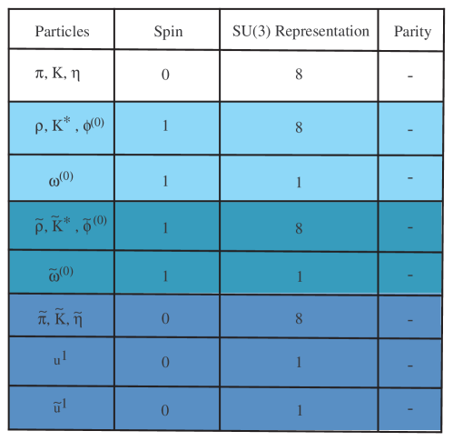
Figure 10: Exact and approximate Goldstone bosons when the effects of next-to-nearest neighbor terms are included.

References

- [1] C.J. Morningstar and M. Weinstein, Phys. Rev. D54, 4131 (1996) hep-lat/9603016. ; Colin J. Morningstar and Marvin Weinstein, Phys. Rev. Lett. 73, 1873 (1994).
- [2] M. Weinstein, Phys. Rev. D 61, 034505 (2000) [arXiv:hep-lat/9910005].
- [3] Phys. Rev. D 14, 1627 (1976).
- [4] K. Melnikov and M. Weinstein, Phys. Rev. D 62, 094504 (2000) [arXiv:hep-lat/0004016].
- [5] M. Weinstein, S. D. Drell, H. R. Quinn and B. Svetitsky, Phys. Rev. D 22, 1190 (1980) and B. Svetitsky, S. D. Drell, H. R. Quinn and M. Weinstein, Phys. Rev. D 22, 490 (1980).