Abstract

We show that the equilibrium positions of the Ruijsenaars-Schneider-van Diejen systems with the trigonometric potential are given by the zeros of the Askey-Wilson polynomials with five parameters. The corresponding single particle quantum version, which is a typical example of “discrete” quantum mechanical systems with a $q$-shift type kinetic term, is shape invariant and the eigenfunctions are the Askey-Wilson polynomials. This is an extension of our previous study [1, 2], which established the “discrete analogue” of the well-known fact; The equilibrium positions of the Calogero systems are described by the Hermite and Laguerre polynomials, whereas the corresponding single particle quantum versions are shape invariant and the eigenfunctions are the Hermite and Laguerre polynomials.

1 Introduction

The Calogero-Sutherland systems [3] and their integrable deformation called the Ruijsenaars-Schneider-van Diejen systems [4, 5] have many attractive features at both classical and quantum mechanical levels. In our recent paper [6, 1], the equilibrium positions of the classical Ruijsenaars-Schneider-van Diejen systems were studied. The equilibrium positions of the Calogero-Sutherland systems are described by the zeros of the classical orthogonal polynomials, the Hermite, Laguerre, Chebyshev, Legendre, Gegenbauer and Jacobi polynomials [7, 8, 9]. Since the Ruijsenaars-Schneider-van Diejen systems are deformation of the Calogero-Sutherland systems, it is expected that the equilibrium positions of the Ruijsenaars-Schneider-van Diejen systems are described by some deformation of these classical orthogonal polynomials. This is indeed the case and we obtained the deformed Hermite, Laguerre and Jacobi polynomials [1]. These deformed orthogonal polynomials fit in the Askey-scheme of the hypergeometric orthogonal polynomials [10, 11]; (i) rational potential cases: One and two parameter deformation of the Hermite polynomials are a special case of the Meixner-Pollaczek polynomial and a special case of the continuous Hahn polynomial, and two and three parameter deformation of the Laguerre polynomials are the continuous dual Hahn polynomial and the Wilson polynomial, (ii) trigonometric potential cases: Several one parameter deformation of the Jacobi polynomials are special cases of the Askey-Wilson polynomial. The Askey-Wilson polynomial has five parameters [12], but the deformed Jacobi polynomials obtained in [1] have only three parameters. A natural question arises; Find (integrable) multi-particle systems whose equilibrium positions are described by the Askey-Wilson polynomials with five parameters.

Shape invariance is an important ingredient of many exactly solvable quantum mechanics [13, 14, 15]. In another recent paper of ours [2], the shape invariance of “discrete” quantum mechanical single particle systems, whose kinetic term causes a shift of the coordinate in the imaginary direction, are discussed. The eigenfunctions of these shape invariant systems are a special case of the Meixner-Pollaczek polynomial, a special case of the continuous Hahn polynomial, the continuous dual Hahn polynomial and the Wilson polynomial. These polynomials have all appeared in the above discussion about the equilibrium positions, in which we have one more polynomial, the Askey-Wilson polynomial. This gives the second question; Are the quantum mechanical single particle systems, whose eigenstates are the Askey-Wilson polynomial, shape invariant or not ?

We will answer the above two questions in this paper. The answer to the first question is found by the same method given in [1], i.e. numerical analysis, functional equation and three-term recurrence. The second question is answered affirmatively by using the properties of the Askey-Wilson polynomials and similar discussion in [2] with replacement of a shift operator by a $q$-shift operator.

This article is organized as follows. In section 2, the classical equilibria of the Ruijsenaars-Schneider-van Diejen system are studied. For a suitable choice of the elementary potential functions, the equilibrium positions are given by the zeros of the Askey-Wilson polynomials with five parameters. In section 3 we discuss the shape invariance of “discrete” quantum mechanical single particle systems with a $q$-shift type kinetic term. After discussing general theory, we present an explicit example of such shape invariant systems, in which eigenstates are described by the Askey-Wilson polynomials. The final section is for a summary and comments.

2 Multi-particle Systems: Equilibrium Positions

Let us consider the equilibrium positions of the classical Ruijsenaars-Schneider-van Diejen systems with the trigonometric potential [4, 5], which are integrable deformation of the celebrated Calogero-Sutherland systems of exactly solvable multi-particle quantum mechanics. Its classical Hamiltonian corresponding to the BC root system is the following [5]:

$$H(p,q) =\sum_{j=1}^{n}\left(\cosh p_{j}\,\sqrt{V_{j}(q)\,{V}_{j}^{*}(q)}-\frac{1}{2}\Bigl{(}V_{j}(q)+{V}_{j}^{*}(q)\Bigr{)}\right),$$ (1)

$$V_{j}(q) =w(q_{j})\prod_{k=1\atop k\neq j}^{n}v(q_{j}-q_{k})\,v(q_{j}+q_{k})\qquad(j=1,\ldots,n),$$ (2)

$$v(x) =\frac{\sin(x-ig_{0})}{\sin x}\,,$$ (3)

$$w(x) =\frac{\sin(x-ig_{1})}{\sin x}\,\frac{\sin(x-ig_{2})}{\sin x}\,\frac{\cos(x-ig_{3})}{\cos x}\,\frac{\cos(x-ig_{4})}{\cos x}\,,$$ (4)

where $q={}^{t}(q_{1},\cdots,q_{n})$ and $p={}^{t}(p_{1},\cdots,p_{n})$ are the coordinates and conjugate momenta, and $g_{j}$ ($j=0,\ldots,4$) are the real positive coupling constants. The potentials $V_{j}$ and $V_{j}^{*}$ are complex conjugate of each other. Our convention of a complex conjugate function is the following: for an arbitrary function $f(x)=\sum_{n}a_{n}x^{n}$ ($a_{n}\in\mathbb{C}$), we define $f^{*}(x)=\sum_{n}a_{n}^{*}x^{n}$. Here $c^{*}$ is the complex conjugation of a number $c\in\mathbb{C}$. Note that $f^{*}(x)$ is not the complex conjugation of $f(x)$, $(f(x))^{*}=f^{*}(x^{*})$. This is relevant for considering complex variables in section 3. The equilibrium positions $p=0$, $q=\bar{q}$ are determined by the condition [6]

$$V_{j}(\bar{q})=V_{j}^{*}(\bar{q})>0\qquad(j=1,2,\ldots,n).$$ (5)

This equation without inequality is rewritten in the Bethe ansatz like equation

$$\prod_{k=1\atop k\neq j}^{n}\frac{v(\bar{q}_{j}-\bar{q}_{k})v(\bar{q}_{j}+\bar{q}_{k})}{v^{*}(\bar{q}_{j}-\bar{q}_{k})v^{*}(\bar{q}_{j}+\bar{q}_{k})}=\frac{w^{*}(\bar{q}_{j})}{w(\bar{q}_{j})}\,.$$ (6)

Note that $\bar{q}_{j}=0,\frac{\pi}{2}$ is excluded in (5) but allowed in (6).

By the same method given in [1] (numerical analysis, functional equation and three-term recurrence), we can show that the equilibrium positions $\{\bar{q}_{j}\}$ are given by the zeros of the Askey-Wilson polynomial [12] (we follow the notation of Koekoek and Swarttouw [11]) $p_{n}(x;a,b,c,d|q)\propto\prod_{j=1}^{n}(x-\cos 2\bar{q}_{j})$ with the following parameters,

$$q=e^{-2g_{0}},\quad(a,b,c,d)=(e^{-2g_{1}},e^{-2g_{2}},-e^{-2g_{3}},-e^{-2g_{4}}).$$ (7)

The outline of derivation is as follows. The functional equation for $f(x)=\prod_{j=1}^{n}(x-\cos 2\bar{q}_{j})$ is the same as eq.(A.4)($\epsilon=-1$) in [1] with

$$h(x) =\Bigl{(}{\textstyle\frac{q^{-1}-q}{2}}x-i(1+{\textstyle\frac{q^{-1}+q}{2}})\sqrt{1-x^{2}}\Bigr{)}$$

$$\quad\times\Bigl{(}{\textstyle\frac{a^{-1}-a}{2}}(1+x)+i(1+{\textstyle\frac{a^{-1}+a}{2}})\sqrt{1-x^{2}}\Bigr{)}\Bigl{(}{\textstyle\frac{b^{-1}-b}{2}}(1+x)+i(1+{\textstyle\frac{b^{-1}+b}{2}})\sqrt{1-x^{2}}\Bigr{)}$$

$$\quad\times\Bigl{(}{\textstyle\frac{c-c^{-1}}{2}}(1-x)-i(1-{\textstyle\frac{c+c^{-1}}{2}})\sqrt{1-x^{2}}\Bigr{)}\Bigl{(}{\textstyle\frac{d-d^{-1}}{2}}(1-x)-i(1-{\textstyle\frac{d+d^{-1}}{2}})\sqrt{1-x^{2}}\Bigr{)},$$ (8)

$$g_{n}(x) =\frac{(1+a)(1+b)(1-c)(1-d)(1+q)(1-x^{2})}{8abcdq^{n+1}}$$

$$\quad\times\Bigl{(}4q(1+abcdq^{2n-1})x^{2}-2q^{n}\bigl{(}abc+abd+acd+bcd+(a+b+c+d)q\bigr{)}x$$

$$\quad\qquad-(1+q)\bigl{(}1+q-q^{n+1}-(ab+ac+ad+bc+bd+cd)q^{n}$$

$$\quad\qquad\qquad\qquad\quad-q^{n-1}(1-q^{n}-q^{n+1})abcd\bigr{)}\Bigr{)},$$ (9)

and $\sqrt{\delta}=\frac{1-q}{1+q}$. The three-term recurrence $f_{n+1}(x)=(x-a_{n})f_{n}(x)-b_{n}f_{n-1}(x)$ for the monic Askey-Wilson polynomial can be found in the literature, for example eq.(3.1.5) in [11]. Then eq.(A.7) in [1] holds because the functions $X_{n}(x),Y_{n}(x)$ of (A.13),(A.14) in [1] vanish for these $a_{n},b_{n}$ and $g_{n}(x)$. Therefore we obtain Proposition A.3, A.4 in [1].

Remark 1: The models studied in [1] are special cases of this model. For example,

$$B (g_{0},g_{1},g_{2},g_{3},g_{4})=(g_{L},{\textstyle\frac{1}{2}}g_{S},{\textstyle\frac{1}{2}}g_{S},0,0),$$ eq.(2.75) in [1]

$$C^{\prime} (g_{0},g_{1},g_{2},g_{3},g_{4})=(g_{S},{\textstyle\frac{1}{2}}g_{L},{\textstyle\frac{1}{2}}g_{L},{\textstyle\frac{1}{2}}g_{L},{\textstyle\frac{1}{2}}g_{L}),$$ eq.(2.78) in [1]

$$B^{\prime}C (g_{0},g_{1},g_{2},g_{3},g_{4})=(g_{M},g_{S},g_{L},g_{L},0),$$ eq.(2.79) in [1]

due to the following trigonometric formulas,

$$\frac{\sin(x-ig)}{\sin x}=\cosh g\,(1-i\tanh g\cot x),\quad\frac{\cos(x-ig)}{\cos x}=\cosh g\,(1+i\tanh g\tan x),$$

$$\cosh 2g(1-i\tanh 2g\cot 2x)=\frac{\sin(2x-i2g)}{\sin 2x}=\frac{\sin(x-ig)}{\sin x}\,\frac{\cos(x-ig)}{\cos x}.$$

Remark 2: Ismail et.al. studied the $q$-Strum Liouville problems and the Bethe ansatz equation of the XXZ model [16]. A special case of their results states that the zeros of Askey-Wilson polynomial $p_{n}(x;a,b,c,d|q)\propto\prod_{j=1}^{n}(x-\cos 2\bar{q}_{j})$ with the parameters

$$q=e^{-2g_{0}},\quad(a,b,c,d)=(e^{-2g_{1}},e^{-2g_{2}},e^{-2g_{3}},e^{-2g_{4}}),$$ (10)

satisfies the Bethe ansatz like equation (6) with ($g_{j}>0$)

$$v(x)=\frac{\sin(x-ig_{0})}{\sin x}\,,\quad w(x)=\frac{\sin(x-ig_{1})}{\sin x}\,\frac{\sin(x-ig_{2})}{\sin x}\,\frac{\sin(x-ig_{3})}{\sin x}\,\frac{\sin(x-ig_{4})}{\sin x}\,.$$ (11)

However this does not mean that $\{\bar{q}_{j}\}$ are equilibrium positions of the system (1) with (11), because $V_{j}(\bar{q})$ is not positive in this case. Moreover the $\cot^{4}x$ term in $w(x)$ (11) appears too singular to give a satisfactory quantum Hamiltonian.

3 Single Particle Systems: Shape Invariance

Next let us consider the shape invariance of the “discrete” quantum mechanical single particle systems with a $q$-shift type kinetic term. The argument is parallel to that given in [2], in which discrete quantum systems with a shift-type kinetic term are discussed.

In this section we use variables $\theta$, $x$ and $z$, which are related as

$$0\leq\theta\leq\pi,\quad x=\cos\theta,\quad z=e^{i\theta}.$$ (12)

The dynamical variable is $2\theta$ and the inner product is $(f(\theta),g(\theta))=\int_{0}^{\pi}d\theta f(\theta)^{*}g(\theta)$. We denote $D=D_{z}\stackrel{{\scriptstyle\rm def}}{{=}}z\frac{d}{dz}$. Then $q^{D}$ is a $q$-shift operator, $q^{D}f(z)=f(qz)$. Note that

$$\int_{0}^{\pi}d\theta=\int_{-1}^{1}\frac{dx}{\sqrt{1-x^{2}}},\quad-i\frac{d}{d\theta}=z\frac{d}{dz}=D,\quad f(z)^{*}=f^{*}(z^{-1}).$$ (13)

For a real constant $q$ ($0<q<1$) and a function $V(z)=V(z;\bm{\lambda},q)$ with a set of real parameters $\bm{\lambda}$, let us consider the following Hamiltonian $H=H(z;\bm{\lambda},q)$,

$$H\stackrel{{\scriptstyle\rm def}}{{=}}{\textstyle\frac{1}{2}}\sqrt{V(z)}\,q^{D}\!\sqrt{V^{*}(z^{-1})}+{\textstyle\frac{1}{2}}\sqrt{V^{*}(z^{-1})}\,q^{-D}\!\sqrt{V(z)}-{\textstyle\frac{1}{2}}(V(z)+V^{*}(z^{-1})).$$ (14)

The eigenvalue equation reads

$$H\phi_{n}=\mathcal{E}_{n}\phi_{n},$$ (15)

with eigenfunctions $\phi_{n}(z)=\phi_{n}(z;\bm{\lambda},q)$ and eigenvalues $\mathcal{E}_{n}=\mathcal{E}_{n}(\bm{\lambda},q)$ ($n=0,1,\ldots$) (we assume non-degeneracy $\mathcal{E}_{0}<\mathcal{E}_{1}<\cdots$). The kinetic term causes a $q$-shift in the variable $z$. This Hamiltonian is factorized and consequently positive semi-definite:

$$H =A^{\dagger}A,$$ (16)

$$A =A(z;\bm{\lambda},q)\stackrel{{\scriptstyle\rm def}}{{=}}\frac{1}{\sqrt{2}}\Bigl{(}q^{\frac{D}{2}}\sqrt{V^{*}(z^{-1})}-q^{-\frac{D}{2}}\sqrt{V(z)}\Bigr{)},$$ (17)

$$A^{\dagger} =A(z;\bm{\lambda},q)^{\dagger}\stackrel{{\scriptstyle\rm def}}{{=}}\frac{1}{\sqrt{2}}\Bigl{(}\sqrt{V(z)}\,q^{\frac{D}{2}}-\sqrt{V^{*}(z^{-1})}\,q^{-\frac{D}{2}}\Bigr{)},$$ (18)

where $\dagger$ denotes the hermitian conjugation with respect to the above inner product. The ground state $\phi_{0}$ is the function annihilated by $A$:

$$A\phi_{0}=0\quad(\Rightarrow H\phi_{0}=0,\ {\cal E}_{0}=0).$$ (19)

Explicitly this equation reads

$$\sqrt{V^{*}(q^{-\frac{1}{2}}z^{-1})}\,\phi_{0}(q^{\frac{1}{2}}z)=\sqrt{V(q^{-\frac{1}{2}}z)}\,\phi_{0}(q^{-\frac{1}{2}}z).$$ (20)

The other eigenfunctions can be obtained in the form

$$\phi_{n}(z)\propto P_{n}(z)\phi_{0}(z),$$ (21)

where $P_{n}(z)=P_{n}^{(\bm{\lambda},q)}(z)$ is a Laurent polynomial in $z$ (for the explicit example below, it is the Askey-Wilson polynomial in $x$). This $P_{n}(z)$ satisfies

$$\tilde{H}P_{n}=\mathcal{E}_{n}P_{n}.$$ (22)

Here $\tilde{H}=\tilde{H}(z;\bm{\lambda},q)$ is a similarity transformed Hamiltonian in terms of the ground state wavefunction $\phi_{0}$:

$$\tilde{H}\stackrel{{\scriptstyle\rm def}}{{=}}\phi_{0}^{-1}\circ H\circ\phi_{0}={\textstyle\frac{1}{2}}V(z)\,q^{D}+{\textstyle\frac{1}{2}}V^{*}(z^{-1})\,q^{-D}-{\textstyle\frac{1}{2}}(V(z)+V^{*}(z^{-1})).$$ (23)

Corresponding to the factorization of $H$ (16), $\tilde{H}$ is also factorized:

$$\tilde{H} =BC,$$ (24)

$$C =C(z,q)={\textstyle\frac{1}{2}}(q^{\frac{D}{2}}-q^{-\frac{D}{2}}),$$ (25)

$$B =B(z;\bm{\lambda},q)=V(z)\,q^{\frac{D}{2}}-V^{*}(z^{-1})\,q^{-\frac{D}{2}}.$$ (26)

Let us define a new set of wavefunctions $\phi_{1,n}(z)=\phi_{1,n}(z;\bm{\lambda},q)$,

$$\phi_{1,n}\stackrel{{\scriptstyle\rm def}}{{=}}A\phi_{n}\quad(n=1,2,\ldots).$$ (27)

As a consequence of the factorization, they form eigenfunctions of a new Hamiltonian $H_{1}=H_{1}(z;\bm{\lambda},q)$,

$$H_{1}=AA^{\dagger}$$ (28)

with the same eigenvalues $\{\mathcal{E}_{n}\}$:

$$H_{1}\phi_{1,n}=AA^{\dagger}A\phi_{n}=A\mathcal{E}_{n}\phi_{n}=\mathcal{E}_{n}\phi_{1,n}\quad(n=1,2,\ldots).$$ (29)

To consider the shape invariance of $H$, we try to find the operators $A_{1}$, $A_{1}^{\dagger}$ and a real constant $\mathcal{E}_{1}$ satisfying

$$H_{1} =AA^{\dagger}=A_{1}^{\dagger}A_{1}+{\cal E}_{1},$$ (30)

$$A_{1} =A_{1}(z;\bm{\lambda},q)\stackrel{{\scriptstyle\rm def}}{{=}}\frac{1}{\sqrt{2}}\Bigl{(}q^{\frac{D}{2}}\sqrt{V_{1}^{*}(z^{-1})}-q^{-\frac{D}{2}}\sqrt{V_{1}(z)}\Bigr{)},$$ (31)

$$A_{1}^{\dagger} =A_{1}(x;\bm{\lambda},q)^{\dagger}\stackrel{{\scriptstyle\rm def}}{{=}}\frac{1}{\sqrt{2}}\Bigl{(}\sqrt{V_{1}(z)}\,q^{\frac{D}{2}}-\sqrt{V_{1}^{*}(z^{-1})}\,q^{-\frac{D}{2}}\Bigr{)}.$$ (32)

In other words, given $V(z)=V(z;\bm{\lambda},q)$, find a new potential $V_{1}(z)=V_{1}(z;\bm{\lambda},q)$ satisfying

$$V_{1}(z)V_{1}^{*}(q^{-1}z^{-1})=V(q^{\frac{1}{2}}z)V^{*}(q^{-\frac{1}{2}}z^{-1}),$$ (33)

$$V_{1}(z)+V_{1}^{*}(z^{-1})=V(q^{-\frac{1}{2}}z)+V^{*}(q^{-\frac{1}{2}}z^{-1})+2{\cal E}_{1}.$$ (34)

If $V_{1}$ has the same functional form as $V$ with another set of parameters $\bm{\lambda}^{\prime}$ (e.g, $q$-shifted $\bm{\lambda}$),

$$V_{1}(z;\bm{\lambda},q)\propto V(z;\bm{\lambda}^{\prime},q),$$ (35)

then it is shape invariant. Suppose $V_{1}$ has the form

$$V_{1}(z)=V(q^{\frac{1}{2}}z)g(z),$$ (36)

with an as yet unspecified function $g(z)$, the above conditions (33), (34) get slightly simplified:

$$g(z)g^{*}(q^{-1}z^{-1})=1,$$ (37)

$$V(q^{\frac{1}{2}}z)g(z)+V^{*}(q^{\frac{1}{2}}z^{-1})g^{*}(z^{-1})=V(q^{-\frac{1}{2}}z)+V^{*}(q^{-\frac{1}{2}}z^{-1})+2{\cal E}_{1}.$$ (38)

If the desired $V_{1}$ is found, we can construct $H_{2},H_{3},\cdots$ by repeating the same step. We illustrate this procedure by taking the Askey-Wilson polynomial as an example.

Let us take $V$ as

$$V(z)=V(z;\bm{\lambda},q)=\frac{(1-az)(1-bz)(1-cz)(1-dz)}{(1-z^{2})(1-qz^{2})},$$ (39)

where $\bm{\lambda}=(a,b,c,d)$. For simplicity we assume $-1<a,b,c,d<1$. Note that $V^{*}(z)=V(z)$. The ground state (19) is given by [11]

$$\phi_{0}(z)=\phi_{0}(z;\bm{\lambda},q)\propto \sqrt{w(z;\bm{\lambda},q)}\stackrel{{\scriptstyle\rm def}}{{=}}\left|\frac{(z^{2};q)_{\infty}}{(az,bz,cz,dz;q)_{\infty}}\right|$$ (40)

$$=\sqrt{\frac{(z^{2},z^{-2};q)_{\infty}}{(az,az^{-1},bz,bz^{-1},cz,cz^{-1},dz,dz^{-1};q)_{\infty}}}\,,$$ (41)

where $(a_{1},\cdots,a_{m};q)_{\infty}=\prod_{j=1}^{m}\prod_{n=0}^{\infty}(1-a_{j}q^{n})$. Excited states have the form (21) $\phi_{n}(z)\propto P_{n}(z)\phi_{0}(z)$, and (22) implies that $P_{n}(z)$ is proportional to the Askey-Wilson polynomial [11],

$$P_{n}(z)=P_{n}^{(\bm{\lambda},q)}(z)\propto p_{n}(x;a,b,c,d;q),$$ (42)

$$\mathcal{E}_{n}=\mathcal{E}_{n}(\bm{\lambda},q)={\textstyle\frac{1}{2}}q^{-n}(1-q^{n})(1-abcdq^{n-1}),$$ (43)

which is an orthogonal polynomial,

$$\int_{-1}^{1}\frac{dx}{\sqrt{1-x^{2}}}\,w(z;\bm{\lambda},q)\,p_{n}(x;a,b,c,d|q)\,p_{m}(x;a,b,c,d|q)\propto\delta_{nm},$$ (44)

namely $(\phi_{n},\phi_{m})\propto\delta_{nm}$. By denoting $p_{n}(x;a,b,c,d|q)=P_{n}(z;\bm{\lambda},q)$, the factorization (24) gives the forward and backward shift relations ((3.1.8) and (3.1.10) in [11]):

$$C(z;q)P_{n}(z;\bm{\lambda},q)=-{\cal E}_{n}(\bm{\lambda},q)q^{\frac{n}{2}}(z-z^{-1})P_{n-1}(z;q^{\frac{1}{2}}\bm{\lambda},q),$$ (45)

$$-B(z;\bm{\lambda},q)\ q^{\frac{n}{2}}(z-z^{-1})P_{n-1}(z;q^{\frac{1}{2}}\bm{\lambda},q)=P_{n}(z;\bm{\lambda},q).$$ (46)

It is easy to check that $V_{1}$ in the form (36) with

$$g(z)=q^{-1}\frac{1-q^{2}z^{2}}{1-z^{2}}$$ (47)

satisfies (37) and (38), and it becomes

$$V_{1}(z;\bm{\lambda},q)=V(q^{\frac{1}{2}}z)g(z)=q^{-1}V(z;q^{\frac{1}{2}}\bm{\lambda},q),$$ (48)

and $\mathcal{E}_{1}$ is

$$\mathcal{E}_{1}(\bm{\lambda},q)=\frac{1}{2}q^{-1}(1-q)(1-abcd).$$ (49)

Therefore we have shape invariance, (48) and

$$A_{1}(z;\bm{\lambda},q) =q^{-\frac{1}{2}}A(z;q^{\frac{1}{2}}\bm{\lambda},q),$$ (50)

$$H_{1}(z;\bm{\lambda},q) =q^{-1}H(z;q^{\frac{1}{2}}\bm{\lambda},q)+\mathcal{E}_{1}(\bm{\lambda},q).$$ (51)

We write down important formulas once again:

$$A(z;\bm{\lambda},q)\phi_{0}(z;\bm{\lambda},q)=0,$$ (52)

$$A(z;\bm{\lambda},q)A(z;\bm{\lambda},q)^{\dagger}=q^{-1}A(z;q^{\frac{1}{2}}\bm{\lambda},q)^{\dagger}A(z;q^{\frac{1}{2}}\bm{\lambda},q)+\mathcal{E}_{1}(\bm{\lambda},q).$$ (53)

Starting from $V_{0}=V$, $H_{0}=H$, $\phi_{0,n}=\phi_{n}$, let us define $V_{s}$, $H_{s}$, $\phi_{s,n}$ ($n\geq s\geq 0$) step by step:

$$V_{s+1}(z;\bm{\lambda},q) \stackrel{{\scriptstyle\rm def}}{{=}}q^{-1}V_{s}(z;q^{\frac{1}{2}}\bm{\lambda},q),$$ (54)

$$H_{s+1}(z;\bm{\lambda},q) \stackrel{{\scriptstyle\rm def}}{{=}}A_{s}(z;\bm{\lambda},q)A_{s}(z;\bm{\lambda},q)^{\dagger}+\mathcal{E}_{s}(\bm{\lambda},q),$$ (55)

$$\phi_{s+1,n}(z;\bm{\lambda},q) \stackrel{{\scriptstyle\rm def}}{{=}}A_{s}(z;\bm{\lambda},q)\phi_{s,n}(z;\bm{\lambda},q).$$ (56)

Here $A_{s}$ and $A_{s}^{\dagger}$ are defined by

$$A_{s}(z;\bm{\lambda},q) \stackrel{{\scriptstyle\rm def}}{{=}}\frac{1}{\sqrt{2}}\Bigl{(}q^{\frac{D}{2}}\sqrt{V_{s}^{*}(z^{-1};\bm{\lambda},q)}-q^{-\frac{D}{2}}\sqrt{V_{s}(z;\bm{\lambda},q)}\Bigr{)},$$ (57)

$$A_{s}(z;\bm{\lambda},q)^{\dagger} \stackrel{{\scriptstyle\rm def}}{{=}}\frac{1}{\sqrt{2}}\Bigl{(}\sqrt{V_{s}(z;\bm{\lambda},q)}\,q^{\frac{D}{2}}-\sqrt{V_{s}^{*}(z^{-1};\bm{\lambda},q)}\,q^{-\frac{D}{2}}\Bigr{)}.$$ (58)

As a consequence of the shape invariance (53), we obtain for $n\geq s\geq 0$,

$$V_{s}(z;\bm{\lambda},q)=q^{-s}V(z;q^{\frac{s}{2}}\bm{\lambda},q),$$ (59)

$$A_{s}(z;\bm{\lambda},q)=q^{-\frac{s}{2}}A(z;q^{\frac{s}{2}}\bm{\lambda},q),\quad A_{s}(z;\bm{\lambda},q)^{\dagger}=q^{-\frac{s}{2}}A(z;q^{\frac{s}{2}}\bm{\lambda},q)^{\dagger},$$ (60)

$$H_{s}(z;\bm{\lambda},q)=A_{s}(z;\bm{\lambda},q)^{\dagger}A_{s}(z;\bm{\lambda},q)+\mathcal{E}_{s}(\bm{\lambda},q)=q^{-s}H(z;q^{\frac{s}{2}}\bm{\lambda},q)+\mathcal{E}_{s}(\bm{\lambda},q),$$ (61)

$$\mathcal{E}_{s+1}(\bm{\lambda},q)=\mathcal{E}_{s}(\bm{\lambda},q)+q^{-s}\mathcal{E}_{1}(q^{\frac{s}{2}}\bm{\lambda},q),$$ (62)

$$H_{s}(x;\bm{\lambda},q)\phi_{s,n}(z;\bm{\lambda},q)=\mathcal{E}_{n}(\bm{\lambda},q)\phi_{s,n}(z;\bm{\lambda},q),$$ (63)

$$A_{s}(z;\bm{\lambda},q)\phi_{s,s}(z;\bm{\lambda},q)=0,$$ (64)

$$A_{s}(x;\bm{\lambda},q)^{\dagger}\phi_{s+1,n}(z;\bm{\lambda},q)=(\mathcal{E}_{n}(\bm{\lambda},q)-\mathcal{E}_{s}(\bm{\lambda},q))\phi_{s,n}(z;\bm{\lambda},q).$$ (65)

The relation (62) means that $\{\mathcal{E}_{n}\}$ is calculable from $\mathcal{E}_{1}$ (49). In other words, the spectrum is determined by the shape invariance.

From (56) and (65) we obtain formulas,

$$\phi_{s,n}(z;\bm{\lambda},q)=A_{s-1}(z;\bm{\lambda},q)\cdots A_{1}(z;\bm{\lambda},q)A_{0}(z;\bm{\lambda},q)\phi_{n}(z;\bm{\lambda},q),$$ (66)

$$\phi_{n}(z;\bm{\lambda},q)=\frac{A_{0}(z;\bm{\lambda},q)^{\dagger}}{\mathcal{E}_{n}(\bm{\lambda},q)-\mathcal{E}_{0}(\bm{\lambda},q)}\,\frac{A_{1}(z;\bm{\lambda},q)^{\dagger}}{\mathcal{E}_{n}(\bm{\lambda},q)-\mathcal{E}_{1}(\bm{\lambda},q)}\cdots\frac{A_{n-1}(z;\bm{\lambda},q)^{\dagger}}{\mathcal{E}_{n}(\bm{\lambda},q)-\mathcal{E}_{n-1}(\bm{\lambda},q)}\,\phi_{n,n}(z;\bm{\lambda},q).$$ (67)

The former (66) gives the eigenfunction $\phi_{s,n}$ of the $s$-th Hamiltonian $H_{s}$ along the isospectral line with energy $\mathcal{E}_{n}$, starting from $\phi_{n}$ of the original Hamiltonian $H$ by repeated application of the $A$ operators. The latter (67), on the other hand, expresses the $n$-th eigenfunction $\phi_{n}$ of the original Hamiltonian, starting from the explicitly known ground state $\phi_{n,n}$ of the $n$-th Hamiltonian $H_{n}$ by repeated application of the $A^{\dagger}$ operators. Since (61) implies $\phi_{n,n}(z;\bm{\lambda},q)\propto\phi_{0}(z;q^{\frac{n}{2}}\bm{\lambda},q)$, $\phi_{n}$ is expressed in terms of $\phi_{0}$ and $V$. The latter formula (67) could also be understood as the generic form of the Rodrigue’s formula for the orthogonal polynomials. The situation is depicted in Fig.1.

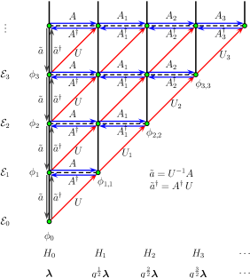
Figure 1: A schematic diagram of the energy levels and the associated Hamiltonian systems together with the definition of the $A$ and $A^{\dagger}$ operators and the ‘creation’ ($\tilde{a}^{\dagger}$) and ‘annihilation’ ($\tilde{a}$) operators. The parameter set is indicated below each Hamiltonian.

The operator $A$ acts to the right and $A^{\dagger}$ to the left along the horizontal (isospectral) line. They should not be confused with the annihilation and creation operators, which act along the vertical line of a given Hamiltonian $H_{s}$ going from one energy level $\mathcal{E}_{n}$ to another $\mathcal{E}_{n\pm 1}$.

In order to define the annihilation and creation operators, let us introduce normalized basis $\{\hat{\phi}_{s,n}\}_{n\geq s}$ for each Hamiltonian $H_{s}$. Ordinarily, the phase of each element of an orthonormal basis could be completely arbitrary. In the present case, however, the eigenfunctions are orthogonal polynomials. That is, they are real and the relations among different degree members are governed by the three-term recurrence relations. So the phases of $\{\hat{\phi}_{s,n}\}_{n\geq s}$ are fixed. Let us introduce a unitary (in fact an orthogonal) operator $U_{s}$ mapping the $s$-th orthonormal basis $\{\hat{\phi}_{s,n}\}_{n\geq s}$ to the $(s+1)$-th $\{\hat{\phi}_{s+1,n}\}_{n\geq s+1}$ (see Fig. 1 and for example [15, 17]):

$$U_{s}\hat{\phi}_{s,n}=\hat{\phi}_{s+1,n+1},\quad U_{s}^{\dagger}\hat{\phi}_{s+1,n+1}=\hat{\phi}_{s,n}.$$ (68)

We denote that $U_{0}=U$. Roughly speaking $U$ changes the parameters from $\bm{\lambda}$ to $q^{\frac{1}{2}}\bm{\lambda}$. Let us introduce an annihilation $\tilde{a}$ and a creation operator $\tilde{a}^{\dagger}$ for the Hamiltonian $H$ as follows:

$$\tilde{a}=\tilde{a}(z;\bm{\lambda},q)\stackrel{{\scriptstyle\rm def}}{{=}}U^{\dagger}A(z;\bm{\lambda},q),\quad\tilde{a}^{\dagger}=\tilde{a}(z;\bm{\lambda},q)^{\dagger}\stackrel{{\scriptstyle\rm def}}{{=}}A(z;\bm{\lambda},q)^{\dagger}U.$$ (69)

It is straightforward to derive

$$H=\tilde{a}^{\dagger}\tilde{a},$$ (70)

$$[\tilde{a},\tilde{a}^{\dagger}]\hat{\phi}_{n}(z;\bm{\lambda},q)=({\cal E}_{n+1}(\bm{\lambda},q)-{\cal E}_{n}(\bm{\lambda},q))\hat{\phi}_{n}(z;\bm{\lambda},q).$$ (71)

4 Summary and Comments

In this article we have studied the equilibrium positions of the Ruijsenaars-Schneider-van Diejen systems with the trigonometric potential and shown that for a suitable choice of the elementary potential functions they are given by the zeros of the Askey-Wilson polynomials with five parameters (see the footnote in section 2). The equation for the equilibrium positions (5) (without the positivity condition) can be written in the Bethe ansatz like equation (6). The Bethe ansatz is a powerful method for solvable models, and solving the Bethe ansatz equation or clarifying the properties of its solutions are very important. Ismail et.al. studied Bethe ansatz equations for spin $s$ XXZ models from the $q$-Sturm-Liouville problem point of view [16]. This kind of approach would shed new light on the Bethe ansatz(-like) equations.

We have also studied the shape invariance of “discrete” quantum mechanical single particle systems with a $q$-shift type kinetic term. As an example of this shape invariance, we present such a system whose eigenfunctions are the Askey-Wilson polynomials. In this example $V(z)$ is a rational function of $z$ (trigonometric function of $\theta$), but the method works for a wider class of functions. In ordinary quantum mechanics there is the Crum’s theorem [14], which states a construction of the associated isospectral Hamiltonians $H_{s}$ and their eigenfunctions $\phi_{s,n}$ (Fig.1) even if the system has no shape invariance. The construction of $H_{s}$ and $\phi_{s,n}$ given in this article and [2] needs shape invariance. A “discrete” analogue of the Crum’s theorem, namely similar construction without shape invariance, would be very helpful, if exists.

We comment on the shape invariance of the Askey-Wilson polynomials with a small number of parameters, $p_{n}(x;a,b,1,-1)$. In this case $V(z)$ in (14) is

$$V(z;\bm{\lambda},q)=\frac{(1-az)(1-bz)}{1-qz^{2}},\quad\bm{\lambda}=(a,b).$$ (72)

By taking a form (36) with the same $g(z)$ (47), the conditions (37) and (38) are satisfied, and we have

$$V_{1}(z;\bm{\lambda},q)=q^{-1}V(q^{-\frac{1}{2}}z;q\bm{\lambda},q),\quad\mathcal{E}_{1}(\bm{\lambda},q)=\frac{1}{2}(q^{-1}-1)(1+ab).$$ (73)

Since $D_{z}=z\frac{d}{dz}$ is invariant under the rescaling of $z$, $D_{z}=D_{\alpha z}$, the Hamiltonian is shape invariant,

$$H_{1}(z,\bm{\lambda},q)=q^{-1}H(q^{-\frac{1}{2}}z;q\bm{\lambda},q)+\mathcal{E}_{1}(\bm{\lambda},q).$$ (74)

The $s$-th Hamiltonian and the spectrum are given by

$$H_{s}(z;\bm{\lambda},q)=q^{-s}H(q^{-\frac{s}{2}}z;q^{s}\bm{\lambda},q)+\mathcal{E}_{s}(\bm{\lambda},q),$$ (75)

$$\mathcal{E}_{s}(\bm{\lambda},q)=\mathcal{E}_{s-1}(\bm{\lambda},q)+q^{-(s-1)}\mathcal{E}_{1}(q^{s-1}\bm{\lambda},q)=\frac{1}{2}q^{-s}(1-q^{s})(1+abq^{s-1}).$$ (76)

References

- [1] S. Odake and R. Sasaki, “Equilibria of ‘Discrete’ Integrable Systems and Deformations of Classical Polynomials”, hep-th/0407155.
- [2] S. Odake and R. Sasaki, “Shape Invariant Potentials in “Discrete Quantum Mechanics””, preprint (Sep. 2004), DPSU-04-3, YITP-04-55, hep-th/0410102.
- [3] F. Calogero, “Solution of the one-dimensional -body problem with quadratic and/or inversely quadratic pair potentials”, J. Math. Phys. 12 (1971) 419-436; B. Sutherland, “Exact results for a quantum many-body problem in one-dimension. II”, Phys. Rev. A5 (1972) 1372-1376.
- [4] S. N. M Ruijsenaars and H. Schneider, “A New Class Of Integrable Systems And Its Relation To Solitons,” Annals Phys. 170 (1986) 370-405; S. N. M Ruijsenaars, “Complete Integrability of Relativistic Calogero-Moser Systems And Elliptic Function Identities,” Comm. Math. Phys. 110 (1987) 191-213.
- [5] J. F. van Diejen, “Integrability of difference Calogero-Moser systems”, J. Math. Phys. 35 (1994) 2983-3004; “The relativistic Calogero model in an external field,” solv-int/ 9509002; “Multivariable continuous Hahn and Wilson polynomials related to integrable difference systems”, J. Phys. A28 (1995) L369-L374; “Difference Calogero-Moser systems and finite Toda chains”, J. Math. Phys. 36 (1995) 1299-1323; “On the Diagonalization of Difference Calogero-Sutherland Systems”, q-alg/9504012.
- [6] O. Ragnisco and R. Sasaki, “Quantum vs Classical Integrability in Ruijsenaars-Schneider Systems,” J. Phys. A37 (2004) 469-479.
- [7] F. Calogero, “On the zeros of the classical polynomials”, Lett. Nuovo Cim. 19 (1977) 505-507; “Equilibrium configuration of one-dimensional many-body problems with quadratic and inverse quadratic pair potentials”, Lett. Nuovo Cim. 22 (1977) 251-253.
- [8] T. Stieltjes, “Sur quelques théorèmes d’Algèbre”, Compt. Rend. 100 (1885) 439-440; “Sur les polynômes de Jacobi”, Compt. Rend. 100 (1885) 620-622; G. Szegö, “Orthogonal polynomials”, Amer. Math. Soc. New York (1939).
- [9] S. Odake and R. Sasaki, “Polynomials Associated with Equilibrium Positions in Calogero-Moser Systems,” J. Phys. A35 (2002) 8283-8314.
- [10] G. E. Andrews, R. Askey and R. Roy, “Special Functions”, Encyclopedia of mathematics and its applications, Cambridge, (1999).
- [11] R. Koekoek and R. F. Swarttouw, “The Askey-scheme of hypergeometric orthogonal polynomials and its -analogue”, math.CA/9602214.
- [12] R. Askey and J. Wilson, “Some basic hypergeometric polynomials that generalize Jacobi polynomials”, Memoirs Aemr. Math. Soc. 319 (1985).
- [13] L. E. Gendenshtein, “Derivation of exact spectra of the Schrodinger equation by means of supersymmetry,” JETP Lett. 38 (1983) 356-359.
- [14] M. M. Crum, “Associated Sturm-Liouville systems”, Quart. J. Math. Oxford Ser. (2) 6 (1955) 121-127, physics/9908019.
- [15] V. Spiridonov, L. Vinet and A. Zhedanov, “Difference Schrodinger operators with linear and exponential discrete spectra,” Lett. Math. Phys. 29 (1993) 63-74.
- [16] M. E. H. Ismail, S. S. Lin and S. S. Roan, “Bethe Ansatz Equations of XXZ Model and q-Sturm-Liouville Problems”, math-ph/0407033.
- [17] A. H. El Kinani and M. Daoud “Generalized coherent and intelligent states for exact solvable quantum systems” J. Math. Phys. 43 (2002) 714-733.
- [18] J. F. van Diejen, “On the Equilibrium Configuration of the -type Ruijsenaars-Schneider System”, math-ph/0410008.