We discuss non-compact $SL(2,\mathbb{R})$ sectors in N=4 SYM and in AdS string theory and compare their integrable structures. We formulate and solve the Riemann-Hilbert problem for the finite gap solutions of the classical sigma model and show that at one loop it is identical to the classical limit of Bethe equations of the spin (-1/2) chain for the dilatation operator of SYM.

1 Introduction

The semiclassical limit of the AdS/CFT correspondence [1, 2] reveals new symmetries which are likely to play an important role in the poorly understood quantum regime of the duality. The semiclassical approximation is accurate for states (closed string states in AdS or local operators in CFT) whose quantum numbers are large. While string theory certainly simplifies in this limit, the necessity to consider operators with large quantum numbers is a complication rather than simplification in the field theory. Such operators contain many constituent fields, are highly degenerate and mix in a complicated way. Fortunately, the operator mixing in ${\cal N}=4$ supersymmetric Yang-Mills (SYM) theory possesses rich hidden symmetries that make the problem tractable. The one-loop planar mixing matrix (dilatation operator) turns out to be a Hamiltonian of an integrable quantum spin chain [3, 4]. The spin-chain Hamiltonian is a member of an infinite series of commuting charges and can be diagonalized by powerful techniques from the Bethe ansatz. The integrability in SYM extends to at least three loops [5, 6, 7, 8] and probably to higher orders of perturbation theory [9]. It is therefore natural to expect that the dual string theory is integrable as well. Turning the argument around, the AdS/CFT duality and the putative quantum integrability of the AdS sigma-model would naturally explain the otherwise miraculous integrability of the operator mixing in SYM [10]. The classical sigma-model on $AdS_{5}\times S^{5}$ is indeed completely integrable [11, 12], but not much is known about the quantum theory.

Even though integrable systems are incomparably simpler than non-integrable, finding the spectrum of a quantum integrable model is still a non-trivial task. To the best of our knowledge, the only tool that possesses sufficient degree of universality is the Bethe ansatz [13, 14, 15]. The classic example of the model solvable by the Bethe ansatz is the Heisenberg spin chain [13, 15]. The Bethe ansatz solution of this model and related spin systems was extremely useful in comparing anomalous dimensions of local operators in SYM [16, 17, 18] to the energies of classical string solitons in $AdS_{5}\times S^{5}$ [19, 20, 21, 22]. The energies were found to agree with the scaling dimensions up to two loops in many particular cases. Higher charges of integrable hierarchies were also identified for particular solutions [28, 29]. The relationship between spin chains and the sigma-model was subsequently established quite generally at the level of effective actions [30, 31, 32, 33, 34, 35, 36], equations of motion [37], or at the level of Bethe ansätze [38].

Although the Bethe ansatz is a purely quantum concept, it leaves certain imprints in the classical dynamics. The classical solutions of the sigma-model can be parameterized by an integral equation that strikingly resembles the scaling limit of Bethe equations for the spin chain [38]. In fact, the two equations become equivalent at weak coupling. This observation lends strong support to the idea that the quantum sigma-model is solvable by the Bethe ansatz. The hypothetical exact Bethe equations for the sigma-model should be discrete, as any quantum Bethe equations, and should reduce to the integral equation derived in [38] in the classical limit. A particular discretization of the classical Bethe equation of [38] was proposed in [39] and passed several non-trivial tests: the equations of [39] reproduce known quantum corrections [23, 24, 25] to the energies of BMN string states [1] and recover the $(g^{2}N)^{1/4}$ asymptotics [40] of anomalous dimensions at strong coupling. Interestingly, the string Bethe equations have a spin chain interpretation [41]. The Bethe equations of [39] are asymptotic in the sense that they require the ’t Hooft coupling and the R-charge to be large, so deriving the full quantum Bethe ansatz for the sigma-model still remains a challenge.

The classical Bethe equations were obtained in [38] for the simplest $SU(2)$ sector of the $AdS_{5}\times S^{5}$ sigma-model which is dual to scalar operators of the form $\,{\rm tr}\,(Z^{J_{1}}W^{J_{2}}+{\rm permutations})$, where $Z=\Phi_{1}+i\Phi_{2}$ and $W=\Phi_{3}+i\Phi_{4}$ are two complex scalars of ${\cal N}=4$ supermultiplet. This sector is closed under renormalization because of the R-charge conservation [42, 43]. On the string side, the $SU(2)$ sector corresponds to strings confined in the $S^{3}\times\mathbb{R}^{1}$ subspace of $AdS_{5}\times S^{5}$. A string in this sector has two independent angular momenta, which are identified with the R-charges $J_{1}$ and $J_{2}$. The $\mathbb{R}^{1}$ direction corresponds to the global AdS time.

In this paper we shall analyze another closed sector with non-compact $SL(2)$ symmetry group. The operators in this sector are composed of an arbitrary number of light-cone covariant derivatives acting on an arbitrary number of scalar fields of one type:

$${\cal O}=\,{\rm tr}\,D_{+}^{S_{1}}Z\ldots D_{+}^{S_{J}}Z,\qquad S_{1}+\ldots+S_{J}=S.$$ (1.1)

where $D_{+}=D_{0}+D_{1}$ and $D_{\mu}=\partial_{\mu}+i[A_{\mu},\ldots],\ \mu=0,1,2,3$. Large operators in this subsector are dual to classical strings that propagate in $AdS_{3}\times S^{1}\subset AdS_{5}\times S^{5}$. The string in $AdS_{3}$ has two independent charges, the Lorentz spin $S$ and the dilatation charge $\Delta$. These charges label representations of $SO(2,2)$, the symmetry group of $AdS_{3}$. The R-charge $J$ of the operator (1.1) corresponds to the angular momentum along $S^{1}$ and the dilatation charge $\Delta$ of the string maps to the scaling dimension of the dual operator.

Perhaps the simplest string solution with the $SL(2)$ symmetry is the folded spinning string at the centre of AdS [2]. Its energy has the same parametric dependence on the spin ($\Delta\propto\ln S$ at large $S$) as the perturbative anomalous dimension of the operator (1.1) with $J=2$, which is now known up to three loops [44]. The coefficient of proportionality interpolates between power series in $\lambda=g^{2}N$ at weak coupling and power series in $1/\sqrt{\lambda}$ at strong coupling [47]. The latter starts from the $O(\sqrt{\lambda})$ term [2]. The situation changes if in addition to spinning in $AdS_{5}$ the string rotates in $S^{5}$ with the angular momentum $J\sim S\gg 1$ [47]. The string energy is then analytic in $\lambda/J^{2}$ and can be directly compared to the anomalous dimension of an operator of the form (1.1) [17]. The one-loop results for the folded string completely agree. The agreement was also established for the pulsating strings (solutions found in [48] and further discussed in [49])[50]. The relationship between effective actions for strings and spins in the $SL(2)$ sector was derived in [34] and was further studied in [51, 52]. In this paper we shall focus on the relationship between integrable structures.

There is an important difference between the $SU(2)$ and $SL(2)$ sectors. In the former case the dilatation charge is the energy of the string and is decoupled from the rest of the dynamics. In the latter case the dilatation generator is a part of the $SO(2,2)$ isometry group and has non-trivial commutation relations with other generators. In this sense the dilatation generator is not much different from other global charges that together form a closed symmetry algebra. This line of thought has proven extremely useful for constructing the dilatation operator on the field-theory side of AdS/CFT [7, 43].

In section 2 we overview the Bethe ansatz solution for the one loop dilatation operator in the $SL(2)$ sector of the $N=4$ SYM theory. Then we derive the classical limit for long operators. The Bethe equations reduce to a Riemann-Hilbert problem in this limit.

In section 3 we describe the so called finite gap solutions of the classical string rotating on the $AdS_{3}\times S_{1}$ space based on the integrability. The problem is again reduced to a solvable Riemann-Hilbert problem for the quasimomentum defined on a two-sheet Riemann surface. The comparison of two Riemann-Hilbert problems in the week coupling region shows the complete one-loop equivalence of the gauge theory and the sigma model.

Sdection 4 contains the general solution of the one loop Bethe equations in the classical limit. The general case is exemplified by the rational solution, which is dual to the circular string [21]. In section 5 the complete solution is constructed for the sigma model. The rational case is treated in some detail. Section 6 is devoted to the discussion.

2 Bethe Ansatz

The operators (1.1) with the same $J$ and $S$ are degenerate at tree level. This degeneracy is lifted by quantum corrections. The conformal operators with definite scaling dimensions are linear combinations of basic operators (1.1) with coefficients that can be computed order by order in perturbation theory. At each order, the conformal operators are eigenvectors of the mixing matrix, whose eigenvalues are the corresponding anomalous dimensions. The size of the mixing matrix rapidly grows with $S$ and $J$, but the problem significantly simplifies at large $N$ when the mixing matrix takes the form of an $sl(2)$ spin chain with $J$ sites. The operators are the states of the spin chain. Each entry $D_{+}^{S_{l}}Z$ in an operator corresponds to a site of a one-dimensional lattice. The sites are cyclically ordered because of the overall trace. $Z$ without derivatives corresponds to an empty site and $D_{+}^{S_{l}}Z$ corresponds to a site in the $S_{l}$-th excited state. The excitations are naturally classified according to the infinite-dimensional spin $s=-1/2$ representation of $sl(2)$. The mixing matrix acts pairwise on the nearest-neighbor sites of the lattice and turns out to coincide with the Hamiltonian of the integrable spin $s=-1/2$ XXX spin chain [42, 4] which is similar to the spin $s=-1$ [53, 54, 55, 56] and $s=-3/2$ [57, 55, 56] chains that describe anomalous dimensions of quasipartonic operators in QCD. The spin chain is solvable by the Bethe ansatz, and the spectrum of anomalous dimensions can be found by solving a set of algebraic equations:

$$\left(\frac{u_{j}-i/2}{u_{j}+i/2}\right)^{J}=\prod_{k\neq j}\frac{u_{j}-u_{k}+i}{u_{j}-u_{k}-i}\,$$ (2.1)

The roots $u_{j}$, $j=1,\ldots,S$ are distinct real numbers. The solutions of Bethe equations that correspond to eigenstates of the mixing matrix satisfy an additional constraint

$$\prod_{j}\frac{u_{j}-i/2}{u_{j}+i/2}=1.$$ (2.2)

This condition takes into account the cyclicity of the trace in (1.1). Bethe states that satisfy this condition have zero total momentum and are invariant under cyclic permutations of the elementary fields. For a given solution of the Bethe equations, the anomalous dimension is determined by

$$\Delta=S+J+\frac{\lambda}{8\pi^{2}}\sum_{j}\frac{1}{u_{j}^{2}+1/4}+O(\lambda^{2}).$$ (2.3)

More details about the Bethe ansatz and its relationship to the anomalous dimensions of $sl(2)$ operators can be found in [4, 42].

We are interested in the scaling limit $S\rightarrow\infty$, $J\rightarrow\infty$ with the ratio $S/J$ held fixed. This scaling limit was discussed for the $SU(2)$ sector in [58, 59, 16, 38]. The $SL(2)$ case can be understood as an analytic continuation in the spin [17], though there are some differences in the reality conditions for Bethe roots. The Bethe roots scale with $J$ as $u_{j}\sim J$. Equating the phases of both sides of (2.1) and expanding in $1/u_{j}$ we get

$$\sum_{k\neq j}\frac{2}{u_{j}-u_{k}}=2\pi n_{j}-\frac{J}{u_{j}}\,.$$ (2.4)

The mode numbers $n_{j}$ arise because one can choose different branches of the logarithm for different Bethe roots. We shall assume that a macroscopic ($\sim J$) number of Bethe roots have equal mode numbers. The distribution of Bethe roots then can be characterized by a continuous density

$$\rho(x)=\sum_{j=1}^{S}\delta\left(x-\frac{u_{j}}{J}\right).$$ (2.5)

The density has a support on a set of disconnected intervals $C_{1},\ldots,C_{K}$ of the real axis. The interval $C_{i}$ is filled by roots with the mode number $n_{i}$ and is centered around $x=1/2\pi n_{i}$. We can also define the resolvent

$$G(x)=\sum_{j=1}^{S}\frac{1}{Jx-u_{j}}=\int dy\,\frac{\rho(y)}{x-y},$$ (2.6)

which is an analytic function of $x$ on the complex plane with cuts along the intervals $C_{i}$. The density, according to the definition (2.5), is normalized as

$$\left.xG(x)\right|_{x=\infty}=\int dx\,\rho(x)=\frac{S}{J}.$$ (2.7)

The scaling limit of Bethe equations translates into an integral equation for the density:

$$2{-\!\!\!\!\!\!\int}dy\,\frac{\rho(y)}{x-y}=2\pi n_{i}-\frac{1}{x}\qquad{\rm for~{}}x\in C_{i},$$ (2.8)

or, in terms of the resolvant,

$$G(x+i0)+G(x-i0)=2\pi n_{i}-\frac{1}{x}\qquad{\rm for~{}}x\in C_{i}.$$ (2.9)

It is also useful to introduce the quasi-momentum

$$p(x)=G(x)+{1\over 2x}\,$$ (2.10)

which satisfies

$$p(x+i0)+p(x-i0)=2\pi n_{i},\qquad x\in C_{i}$$ (2.11)

The momentum condition (2.2) constraints the first moment of the density:

$$\int dx\,\frac{\rho(x)}{x}=-2\pi m,$$ (2.12)

where $m$ is an arbitrary integer. The second moment determines the anomalous dimension:

$$\Delta-S-J=\frac{\lambda}{8\pi^{2}J}\int dx\,\frac{\rho(x)}{x^{2}}\,.$$ (2.13)

The general solution of the integral equation (2.8) is derived in sec. 4. In the next section we shall derive equations analogous to (2.8), (2.7), (2.12) and (2.13) in the classical sigma-model.

3 Classical Strings on $AdS_{3}\times S^{1}$

3.1 The model

As in the discussion of the SYM operators we shall focus on a particular reduction of the full $AdS_{5}\times S^{5}$ sigma-model by considering strings that move in $AdS_{3}\times\mathbb{R}^{1}$. The symmetry algebra of the sigma-model on $AdS_{3}$ is $so(2,2)\sim sl(2)\times sl(2)$. The $AdS_{3}$ space is the group manifold of $SL(2,\mathbb{R})$ and the two $sl(2)$ symmetries act as the left and right group multiplications. We should mention that the $AdS_{3}$ sigma-model with the WZW term is rather well understood [60] but has quite different properties, even at the classical level. The background NS-NS flux of the WZW model couples directly to the classical string world-sheet, unlike the R-R flux of the $AdS_{5}\times S^{5}$ background that is only important in quantum theory.

The string action in the conformal gauge is

$$S_{\sigma}={\sqrt{\lambda}\over 4\pi}\int_{0}^{2\pi}d\sigma\,\int d\tau\,\left[-\partial_{a}X_{i}\partial^{a}X^{i}+\left(\partial_{a}\phi\right)^{2}\right],$$ (3.1)

where $\phi$ is the angle on a big circle of $S_{5}$ and $X_{i}$, $i=-1,0,1,2$ are the $AdS_{3}$ embedding coordinates. They parameterize a hyperboloid in the four-dimensional space with the signature $(++--)$:

$$X_{i}X^{i}=X_{-1}^{2}+X_{0}^{2}-X_{1}^{2}-X_{2}^{2}=X_{+}X_{-}+Y_{+}Y_{-}=1,$$ (3.2)

where we introduced $X_{\pm}=X_{-1}\pm X_{1}$, $Y_{\pm}=X_{0}\pm X_{2}$. All other world-sheet coordinates on $AdS_{5}$ and $S^{5}$ are set to constant values. Classically, this is a consistent reduction. The $SO(2,2)$ symmetry is manifest in the above parametrization.

The equations of motion that follow from (3.1) should be supplemented by Virasoro constraints:

$$\partial_{\pm}X_{i}\partial_{\pm}X^{i}=(\partial_{\pm}\phi)^{2}.$$ (3.3)

where $\sigma_{\pm}=(\tau\pm\sigma)/2$, $\partial_{\pm}=\partial_{\tau}\pm\partial_{\sigma}$. We can always choose the gauge

$$\phi={J\over\sqrt{\lambda}}\,\tau+m\sigma,$$

where $m$ is the winding number, then

$$\partial_{\pm}X_{i}\partial_{\pm}X^{i}=\left(\frac{J}{\sqrt{\lambda}}\pm m\right)^{2}.$$ (3.4)

The angular momentum on $S^{5}$,

$$J=\frac{\sqrt{\lambda}}{2\pi}\int_{0}^{2\pi}d\sigma\,\partial_{0}\phi,$$ (3.5)

should be identified with the number of the $Z$ fields in the operator (1.1).

A point in $AdS_{3}$ defines a group element of $SL(2,\mathbb{R})$:

$$g=X_{-1}+{\bf X}\cdot{\bf s}\equiv\left(\begin{array}[]{cc}X_{-1}+X_{1}&X_{0}-X_{2}\\ -X_{0}-X_{2}&X_{-1}-X_{1}\end{array}\right)\equiv\left(\begin{array}[]{cc}X_{+}&Y_{-}\\ -Y_{+}&X_{-}\end{array}\right)\in SL(2,\mathbb{R}),$$ (3.6)

where ${\bf X}=(X_{0},X_{1},X_{2})$ and ${\bf s}=(i\sigma_{2},\sigma_{3},-\sigma_{1})$. Another useful parametrization of an $SL(2,\mathbb{R})$ group element is

$$g=e^{iu\sigma_{2}}e^{\rho\sigma_{3}}e^{iv\sigma_{2}}=\left(\begin{array}[]{cc}\cos t\cosh\rho+\cos\psi\sinh\rho&\sin t\cosh\rho-\sin\psi\sinh\rho\\ -\sin t\cosh\rho-\sin\psi\sinh\rho&\cos t\cosh\rho-\cos\psi\sinh\rho\end{array}\right)$$ (3.7)

where $t$ is the global AdS time, $\rho$ is the radial variable and $\psi$ is an angle. $u$ and $v$ are the light-cone coordinates:

$$u={1\over 2}(t+\psi),\qquad v={1\over 2}(t-\psi).$$ (3.8)

The differential on the group manifold has the following form:

$$g^{-1}dg=\left(\begin{array}[]{cc}X_{-}dX_{+}-Y_{+}dY_{+}&X_{-}dY_{-}+Y_{+}dX_{-}\\ -Y_{-}dX_{+}-X_{+}dY_{+}&-Y_{-}dY_{-}+X_{+}dX_{-}\end{array}\right)\in sl(2,\mathbb{R}).$$ (3.9)

The invariant metric then is

$$ds^{2}=-\frac{1}{2}\,{\rm tr}\,(g^{-1}dg)^{2}=dX_{-1}^{2}+dX_{0}^{2}-dX_{1}^{2}-dX_{2}^{2}=\cosh^{2}\rho\ dt^{2}-d\rho^{2}-\sinh^{2}\rho\ d\psi^{2}$$ (3.10)

The time coordinate is an angular variable in the parameterization (3.7). As a consequence, $t(\sigma,\tau)$ is not necessarily periodic in $\sigma$ even if $g(\sigma,\tau)$ is periodic. This makes boundary conditions a non-trivial issue. Just requiring that $g(\sigma+2\pi,\tau)=g(\sigma,\tau)$ is not sufficient because this condition allows the string to wind around the time direction. We will return to the issue of the time-like windings later.

Let us now figure out which global charges in the SYM correspond to Noether charges of the left and right group multiplications in $SL(2,\mathbb{R})$. The boundary of $AdS_{3}$ is located at $\rho\to\infty$. Asymptotically, the metric takes the form

$$ds^{2}={e^{2\rho}\over r^{2}}\left(dr^{2}-r^{2}d\psi^{2}\right),\qquad t=\log r,$$ (3.11)

and is conformal to the two-dimensional Minkowski metric. The rescalings $r\to\Lambda r$ or, in the original variables, $t\to t+\epsilon$ act as dilatations on the boundary. The associated conserved charge should be identified with the scaling dimension $\Delta$ of the operator (1.1). The $U(1)$ rotations $\psi\to\psi+\epsilon^{\prime}$ correspond to boosts in $x^{1}$ direction, under which $D_{+}$ in (1.1) transforms as $D_{+}\to{\,\rm e}\,^{-i\epsilon^{\prime}}D_{+}$. The $U(1)$ charge in the sigma-model thus corresponds to the spin $S$ of the SYM operator.

In the representation (3.7), the scaling transformations correspond to simultaneous left and right multiplication by ${\,\rm e}\,^{i\epsilon\sigma_{2}/2}$. The boosts are generated by the left multiplication by ${\,\rm e}\,^{i\epsilon^{\prime}\sigma_{2}/2}$ and the right multiplication by ${\,\rm e}\,^{-i\epsilon^{\prime}\sigma_{2}/2}$. The Noether currents of left/right group multiplications are

$$j_{a}=g^{-1}\partial_{a}g={1\over 2}\,j^{A}_{a}s^{A},\qquad l_{a}=g^{-1}j_{a}g=\partial_{a}gg^{-1}={1\over 2}\,l^{A}_{a}s^{A},\qquad a=0,1=\tau,\sigma.$$ (3.12)

Therefore,

$$\Delta+S=\frac{\sqrt{\lambda}}{4\pi}\int_{0}^{2\pi}d\sigma\,j^{0}_{0},\qquad\Delta-S=\frac{\sqrt{\lambda}}{4\pi}\int_{0}^{2\pi}d\sigma\,l^{0}_{0}.$$ (3.13)

Finally, the Virasoro constraints (3.4) become

$${1\over 2}\,{\rm tr}\,j_{\pm}^{2}=-\left(\frac{J}{\sqrt{\lambda}}\pm m\right)^{2},$$ (3.14)

where $j_{\pm}=g^{-1}\partial_{\pm}g$.

3.2 Equations of motion and integrability

We shall analyze the classical solutions of the $\sigma$-model on $AdS_{3}\times S^{1}$ along the same lines as solutions of the $SU(2)$ sigma model were analyzed in [38]. According to (3.10), we can write the action (3.1) in the form

$$S_{\sigma}=\frac{\sqrt{\lambda}}{4\pi}\int d\sigma d\tau\,\left[\frac{1}{2}\,\,{\rm tr}\,j_{a}^{2}+(\partial_{a}\phi)^{2}\right].$$ (3.15)

The equation of motion for the $S^{1}$ coordinate is just the Laplace equation

$$\partial_{+}\partial_{-}\phi=0$$

and is solved by $\phi=J\tau/\sqrt{\lambda}+m\sigma$.

The equations of motion for the $sl(2)$ currents can be written as follows

$$\partial_{+}j_{-}+\partial_{-}j_{+}=0,\qquad\partial_{+}j_{-}-\partial_{-}j_{+}+[j_{+},j_{-}]=0.$$ (3.16)

where the last equation is a consequence of the definition (3.12). The equations of motion can be reformulated as the flatness condition [62] for a one-parametric family of currents $J(x)$:

$$J_{\pm}(x)=\frac{j_{\pm}}{1\mp x}\,.$$ (3.17)

If (3.16) are satisfied, then

$$\partial_{+}J_{-}-\partial_{-}J_{+}+[J_{+},J_{-}]=0.$$ (3.18)

The converse is also true. If the connection $J_{a}(x)$ is flat for any $x$, the current $j_{a}$ solves the equations of motion (3.16).

The zero-curvature representation effectively linearizes the problem. Instead of analyzing the equations of motion, which are non-linear, we can study the auxiliary linear problem:

$${\cal L}\Psi\equiv\left(\partial_{\sigma}+{1\over 2}\left({j_{+}\over 1-x}-{j_{-}\over 1+x}\right)\right)\Psi=0,$$ (3.19)

$${\cal M}\Psi\equiv\left(\partial_{\tau}+{1\over 2}\left({j_{+}\over 1-x}+{j_{-}\over 1+x}\right)\right)\Psi=0,$$ (3.20)

for which (3.18) is the consistency condition.

The solution of (3.19) with the initial condition $\Psi(\tau,0)=1$ defines the monodromy matrix:

$$\Omega(x)=P\exp\int_{0}^{2\pi}d\sigma\,{1\over 2}\left({j_{-}\over 1+x}-{j_{+}\over 1-x}\right),$$ (3.21)

and the quasi-momentum $p(x)$:

$$\,{\rm tr}\,\Omega(x)=2\cos p(x).$$ (3.22)

Since the trace of the holonomy of a flat connection does not depend on the contour of integration, the quasi-momentum does not depend on $\tau$, in other words, $p(x)$ is conserved. The quasi-momentum $p(x)$ depends on a parameter and thus generates an infinite set of integrals of motion, for instance by Taylor expansion in $x$.

The complete linear problem (3.19), (3.20) and hence the solution of the original non-linear equations can be reconstructed from the quasi-momentum provided that it satisfies certain analyticity conditions. The procedure, sometimes called the inverse-scattering transformation, is described in detail in [63]. We will not use the full machinery of this method. It will be sufficient for our purposes to derive the analyticity constraints on the quasi-momentum as a function of the spectral parameter.

3.3 Analytic properties of the quasi-momentum

Our exposition closely follows [63] and largely repeats the analysis of the $SU(2)$ sigma-model [38]. There are however some important modifications due to the non-compactness of the target space. The auxiliary problem

$$\left[\partial_{\sigma}+{1\over 2}\left({j_{+}\over 1-x}-{j_{-}\over 1+x}\right)\right]\psi=0$$ (3.23)

resembles one-dimensional Dirac equations (now $\psi$ is a column vector as opposed to (3.19), where $\Psi$ was a two-by-two matrix). It has two linearly independent solutions which can be chosen quasi-periodic. It is useful to see how quasi-periodicity is related to the monodromy matrix. If the initial conditions are its eigenvalues

$$\Omega(x)\psi_{\pm}(x;0)={\,\rm e}\,^{\pm ip(x)}\psi_{\pm}(x;0),$$ (3.24)

the solution $\psi_{\pm}(x;\sigma)=\Psi(x;\sigma)\psi_{\pm}(x;0)$ will satisfy $\psi_{\pm}(x;\sigma+2\pi)={\,\rm e}\,^{\pm ip(x)}\psi_{\pm}(x;\sigma)$ because $\Psi(x;\sigma+2\pi)=\Psi(x;\sigma)\Omega(x)$.

Since the monodromy matrix $\Omega(x)\in SL(2,\mathbb{R})$, $\cos p(x)$ is real for real $x$, but the quasi-momentum itself is not necessarily real. The condition for that is $\,{\rm tr}\,\Omega(x)\leq 2$. Then the quasi-periodic solutions are delta-function normalizable. This corresponds to allowed zones of the one-dimensional Dirac equation (3.23). In the forbidden zones $\,{\rm tr}\,\Omega(x)\geq 2$, the quasi-momentum is imaginary and the wave functions grow exponentially at infinity. The number of forbidden zones is in general infinite, but there is a representative set of solutions (finite-gap solutions) for which this number is finite.

The quasi-momentum $p(x)$ can be analytically continued to complex values of $x$. Its only singularities are at zone boundaries and at $x=\pm 1$, where the potential in (3.23) is singular. Therefore $p(x)$ is a meromorphic function on the complex plane with cuts along the forbidden zones. Let us explain why zone boundaries are branch points. The monodromy matrix generically has two distinct eigenvalues, but at zone boundaries it degenerates into the Jordan cell and has only one eigenvector with the eigenvalue $1$ or $-1$. The quasi-momentum becomes an integer multiple of $\pi$ such that the single quasi-periodic solution of (3.19) is either periodic or anti-periodic. Two linearly independent solutions of (3.23), $\psi_{+}(x,\sigma)$ and $\psi_{-}(x,\sigma)$, collapse into one degenerate solution at zone boundaries and are analytic functions of $x$ elsewhere (except for at $x=\pm 1$). Thus $\psi_{+}(x,\sigma)$ and $\psi_{-}(x,\sigma)$ behave precisely as two branches of a single meromorphic function on a double cover of the complex $x$ plane. The two eigenvalues of the monodromy matrix, ${\,\rm e}\,^{\pm ip(x)}$, are also branches of a single meromorphic function on the hyperelliptic surface the two sheets of which are glued together along the forbidden zones. Another way to see that the quasi-momentum is naturally defined on the Riemann surface is to notice that (3.22) is a quadratic equation for ${\,\rm e}\,^{ip(x)}$. The trace of the monodromy matrix is an entire function of $x$, but its eigenvalues have square root singularities when the discriminant of the equation (3.22) turns to zero, and this happens precisely at zone boundaries when $\,{\rm tr}\,\Omega=2$.

To summarize, the eigenvalues of the monodromy matrix ${\,\rm e}\,^{\pm ip(x)}$ are branches of a single meromorphic function on the hyperelliptic Riemann surface. A particular branch $p(x)$ is analytic on the complex plane with cuts along the forbidden zones. We shall identify these cuts with the intervals on which Bethe roots of the spin chain condense.

3.4 Finite gap solution and asymptotic conditions

Consider now the behavior of the quasi-momentum near one of the forbidden zones. The values of ${\,\rm e}\,^{ip(x)}$ on the two sides of the cut, ${\,\rm e}\,^{ip(x+i0)}$ and ${\,\rm e}\,^{ip(x-i0)}$, are two independent solutions of (3.22). Since $\Omega(x)$ is unimodular, ${\,\rm e}\,^{ip(x+i0)}{\,\rm e}\,^{ip(x-i0)}=1$, and the quasi-momentum satisfies the equation equivalent to (2.11):

$$p(x+i0)+p(x-i0)=2\pi n_{k},\qquad x\in C_{k},$$ (3.25)

which holds on each of the forbidden zones. The integer $n_{k}-n_{k-1}-1$ is the number of (anti)-periodic solutions within the $k$-th allowed zone, that is, the number of the double points between $C_{k-1}$ and $C_{k}$.

The auxiliary linear problem (3.19), (3.20) becomes singular at $x=\pm 1$ and the quasi-momentum develops a pole there. The standard asymptotic analysis yields

$$p(x)=\pi\,\frac{\frac{J}{\sqrt{\lambda}}\mp m}{x\pm 1}+\ldots\qquad(x\rightarrow\mp 1).$$ (3.26)

It can be justified by dropping the non-singular pole term in (3.23), writing the Schrödinger type equation for one of the two components of $\psi$ and solving it in the WKB approximation. The asymptotic analysis determines $p(x)$ only up to a sign. Fixing the sign ambiguity, as in (3.26), excludes a part of solutions, for example pulsating strings of [48, 49, 50]. This point is discussed in more detail in sec. 5.3 of [38].

To express the charges in terms of the spectral data, we expand the quasi-momentum at zero and at infinity. At infinity, ${\cal L}=\partial_{\sigma}-j_{0}/x+\ldots$, and

$$\,{\rm Tr}\,\Omega=2+\frac{1}{2x^{2}}\int_{0}^{2\pi}d\sigma_{1}d\sigma_{2}\,\,{\rm Tr}\,j_{0}(\sigma_{1})j_{0}(\sigma_{2})+\ldots=2-\frac{4\pi^{2}(\Delta+S)^{2}}{\lambda x^{2}}+\ldots\,.$$ (3.27)

Here we assume that the classical solutions correspond to highest-weight states and use (3.13). Thus

$$p(x)=\frac{2\pi(\Delta+S)}{\sqrt{\lambda}\,x}+\ldots\qquad(x\rightarrow\infty).$$ (3.28)

At $x\to 0$, ${\cal L}=\partial_{\sigma}+j_{1}-xj_{0}+\ldots$, which can be written as ${\cal L}=g^{-1}(\partial_{\sigma}-xl_{0}+\ldots)g$. Then,

$$\Omega(x)=g^{-1}(2\pi)P\exp\left(x\int_{0}^{2\pi}d\sigma\,l_{0}+\ldots\right)g(0).$$

Because $g(\sigma)$ is periodic, $g(2\pi)=g(0)$, and thus $\Omega(0)=1$. As we discussed in sec. 3.1, the periodicity of $g(\sigma)$ does not guarantee the periodicity of the AdS time coordinate. The time coordinate is an angular variable in the $SL(2,\mathbb{R})$ parameterization of $AdS_{3}$ and we need to eliminate the unphysical time-like windings by hand. It is easy to see that the integer $p(0)/2\pi$ is precisely the winding number around the time direction: in the simplest case of the string in the middle of AdS ($\rho=0$), $j_{1}=\partial_{\sigma}t$ and $p(0)=t(2\pi)-t(0)$. We thus keep only the solutions with $p(0)=0$. Expanding the quasi-momentum further, we get

$$\,{\rm Tr}\,\Omega=2+\frac{x^{2}}{2}\int_{0}^{2\pi}d\sigma_{1}d\sigma_{2}\,\,{\rm Tr}\,l_{0}(\sigma_{1})l_{0}(\sigma_{2})+\ldots=2-\frac{4\pi^{2}(\Delta-S)^{2}}{\lambda}\,x^{2}+\ldots\,.$$ (3.29)

Hence,

$$p(x)=-\frac{2\pi(\Delta-S)}{\sqrt{\lambda}}\,x+\ldots,\qquad(x\rightarrow 0).$$ (3.30)

The quasi-momentum is a meromorphic function on the complex plane with cuts and has two poles at $x=\pm 1$. Subtracting the singularities at $x\to\pm 1$, we get the function

$$G(x)=p(x)-\pi\left(\frac{\frac{J}{\sqrt{\lambda}}+m}{x-1}+\frac{\frac{J}{\sqrt{\lambda}}-m}{x+1}\right),$$ (3.31)

which is analytic everywhere on the physical sheet. As such, it admits a spectral representation where the spectral density is the discontinuity of $G(x)$ across the cuts: $\rho(x)={\rm Im}G(x)/\pi$. The standard analyticity arguments yield

$$G(x)=\int d\xi\,\frac{\rho(\xi)}{x-\xi}\,.$$ (3.32)

The asymptotic behavior of the resolvent at $x\to\infty$ is determined by (3.28): $G(x)\sim 2\pi[(\Delta+S-J)/\sqrt{\lambda}]/x$, and translates into the normalization condition for the density:

$$\int dx\,\rho(x)=\frac{2\pi}{\sqrt{\lambda}}(\Delta+S-J).$$ (3.33)

The asymptotics at $x\to 0$ follows from (3.30) and yields two other conditions:

$$\int dx\,\frac{\rho(x)}{x^{2}}=\frac{2\pi}{\sqrt{\lambda}}(\Delta-S-J)$$ (3.34)

and

$$\int dx\,\frac{\rho(x)}{x}=-2\pi m.$$ (3.35)

The spectral representation (3.32) and the equation (3.25) imply that the density satisfies a singular integral equation:

$$2{-\!\!\!\!\!\!\int}dy\,\frac{\rho(y)}{x-y}=-2\pi\left(\frac{\frac{J}{\sqrt{\lambda}}+m}{x-1}+\frac{\frac{J}{\sqrt{\lambda}}-m}{x+1}\right)+2\pi n_{k},\qquad x\in{\bf C}_{k}.$$ (3.36)

We obtained a Riemann-Hilbert problem similar to the one appeared in [38] for the $SU(2)$ sector. In fact, if we set the winding number to zero, the equations for the $SU(2)$ sectors can be obtained from the equations for $SL(2,\mathbb{R})$ by an analytic continuation that first appeared in the analysis of particular solutions [17]: $J\rightarrow\Delta$, $S\rightarrow J_{2}$, $\Delta\rightarrow-J_{1}$. This duality is a consequence of the fact that the AdS space can be obtained from the sphere by a double Wick rotation.

3.5 Comparison of string theory to perturbative gauge theory

We are now in a position to compare integral equations that encode periodic solutions of the sigma-model to the scaling limit of Bethe equations that describe anomalous dimensions in SYM. In order to do that we need to get rid of the explicit dependence on the angular momentum $J$ in (3.36). This can be achieved by rescaling the spectral variable $x$ by $4\pi J/\sqrt{\lambda}$:

$$2{-\!\!\!\!\!\!\int}dy\,\frac{\rho(y)}{x-y}=2\pi n_{i}-\frac{x+\frac{m\lambda}{4\pi J^{2}}}{x^{2}-\frac{\lambda}{16\pi^{2}J^{2}}}\,.$$ (3.37)

The normalization conditions (3.33), (3.34) and (3.35) now become

$$\int dx\,\rho(x)=\frac{S}{J}+\frac{\Delta-S-J}{2J},$$ (3.38)

$$\int dx\,\frac{\rho(x)}{x}=-2\pi m,$$ (3.39)

$$\frac{\lambda}{8\pi^{2}J}\int dx\,\frac{\rho(x)}{x^{2}}=\Delta-S-J\,.$$ (3.40)

If $\lambda/J^{2}\rightarrow 0$, we recover indeed the one-loop Bethe equations of sec. 2. In section 5 we will obtain the general solution of this Riemann-Hilbert problem and present explicitly the one-cut solutions. This solution also demonstrates the one-loop equivalence of the string and gauge descriptions. It is interesting that the winding number explicitly enters the right hand side of the Bethe equation, but it enters in the combination with the ’t Hooft coupling and therefore disappears at one loop.

The string Bethe equation agrees with the scaling limit of the gauge Bethe equation up to two loops in the $SU(2)$ sector [38]. The two-loop agreement extends to the $SO(6)$ (strings moving in $S^{5}\times\mathbb{R}$), at least for particular solutions [64]. The derivation involves the change of variables and subsequent expansion in $\lambda/J^{2}$. Let us try to repeat the same steps for the $SL(2)$. The most important difference between the string and the gauge Bethe equations is the normalization of the densities in (3.38) and in (2.7). The density for the spin chain (2.7) just counts the number of spin excitations which we would normally identify with the number of derivatives in the operator (1.1). The normalization is obviously coupling-independent. On the contrary, the normalization of the string density (3.38) depends on the coupling through $\Delta$. This problem can be fixed by using (3.40) and rewriting (3.38) as

$$\int dx\,\rho(x)\left(1-\frac{T}{x^{2}}\right)=\frac{S}{J}\,,\qquad\left(T=\frac{\lambda}{16\pi^{2}J^{2}}\right).$$ (3.41)

The change of variables $x\rightarrow x-T/x$ cancels the unwanted term in the normalization condition, but spoils the Bethe equation, since the change of variables,

$${-\!\!\!\!\!\!\int}dy\,\frac{\rho\left(y+\frac{T}{y}\right)}{x-\frac{T}{x}-y}={-\!\!\!\!\!\!\int}dy\,\frac{\rho(y)}{x-y}+\frac{T}{x}\int\ dy\,\frac{\rho(y)}{y^{2}}+\ldots$$ (3.42)

produces a non-local term which explicitly depends on the density. The other source of non-locality is the winding number that according to (3.39) can also be represented as a moment of the density. Keeping only $O(\lambda/J^{2})$ terms in (3.37) we find:

$$2{-\!\!\!\!\!\!\int}dy\,\frac{\rho(y)}{x-y}=2\pi n_{i}-\frac{1}{x}-\frac{\lambda}{8\pi^{2}J^{2}x^{3}}-\frac{\lambda}{8\pi^{2}J^{2}}\int dy\,\rho(y)\left(\frac{1}{xy^{2}}+\frac{1}{yx^{2}}\right).$$ (3.43)

The last term is non-local. Non-localities of this type cancel out for the $SU(2)$ sigma-model and do not arise in the $SU(2)$ sector of SYM as well. We cannot exclude that the yet unknown two-loop corrections make $SL(2)$ Bethe equations non-local (such non-local terms might in principle originate from corrections to the scattering phases of elementary excitations), but it is also possible that the discrepancies between SYM and strings arise in the $SL(2)$ sector already at two loops.

4 The General Solution of Bethe Equations in the Scaling Limit

Here we use the method proposed in [66] to find the general solution of (2.8). The derivation repeats that for the compact $SU(2)$ spin chain [38] with minor modifications. The quasimomentum defined in (2.10) has a pole at zero and is analytic elsewhere on the complex plane with cuts $C_{i}$. The discontinuity of the quasimomentum across a cut is proportional to the density and the continuous part is fixed by eq. (2.11). The function $p(x)$ is completely determined by its analiticity properties and can be found using the follwing ansatz:

$$dp=\frac{dx}{y}\left(\frac{a_{-2}}{x^{2}}+\frac{a_{-1}}{x}+\ldots+a_{K-2}x^{K-2}\right),$$ (4.1)

where

$$y^{2}=r_{0}+\ldots r_{2K-1}x^{2K-1}+x^{2K}.$$ (4.2)

The quasi-momentum $p(x)$ can now be obtained by integrating $dp/dx$.

So defined, $dp$ is an Abelian differential of the third kind on a hyperelliptic Riemann surface $\Sigma$ of genus $K-1$. The Riemann surface is defined by (4.2). It is obtained by gluing together two copies of the complex plane along the cuts $C_{i}$, $i=1,\ldots,K$. The result of the integration, $p(x)$, must be single-valued on the physical sheet. It is easy to see that single-valuedness of $p(x)$ is equivalent to the vanishing of all $A$-periods of $dp$:

$$\oint_{A_{i}}dp=0,$$ (4.3)

where the $A$-cycles are the contours surrounding the first $K-1$ cuts (fig. 1).

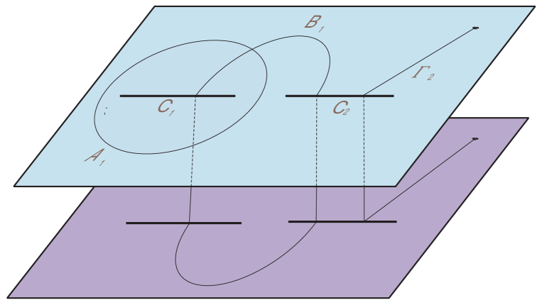
Figure 1: The Riemann surface $\Sigma$ for $K=2$.

The condition (2.11) is equivalent to the integrality of the B-periods of $dp$:

$$\oint_{B_{i}}dp=2\pi(n_{i}-n_{K}),$$ (4.4)

where the $B_{i}$-cycle traverses the $i$th and the $K$th cuts. The B-cycle conditions constitute $K-1$ linear combinations of the original $K$ equations (2.11). The remaining condition determines the integral of $dp$ along the open contour $\Gamma_{K}$ that connects infinite points on the two sheets of the Riemann surface (fig. 1):

$$\int_{\Gamma_{K}}dp=2\pi n_{K}.$$ (4.5)

The Laurent expansion of the quasimomentum at zero generates local charges of the spin chain [28, 18]. In particular:

$$p(x)=\frac{1}{2x}-2\pi m-\frac{8\pi^{2}J(\Delta-S-J)}{\lambda}\,x+\ldots\,\qquad(x\rightarrow 0).$$ (4.6)

The condition that

$$dp\sim-1/2x^{2}+{\rm regular}\qquad(x\rightarrow 0)$$

determines the singular part of $dp$:

$$a_{-2}=-\frac{\sqrt{r_{0}}}{2}\,,\qquad a_{-1}=-\frac{r_{1}}{4\sqrt{r_{0}}}\,.$$ (4.7)

The momentum condition is non-local and requires that

$$\int_{0}^{\infty}dp\in 2\pi\mathbb{Z}.$$ (4.8)

The freedom in choosing the contour of integration leads to an integer-valued ambiguity and thus does not affect the final result. Finally, the $O(1)$ Laurent coefficient of $dp$ determines the anomalous dimension:

$$\Delta-S-J=\frac{\lambda}{8\pi^{2}J}\left(\frac{r_{2}}{4r_{0}}-\frac{r_{1}^{2}}{16r_{0}^{2}}+\frac{a_{1}}{\sqrt{r_{0}}}\right).$$ (4.9)

Counting the parameters we see that this is the general solution of the integral equation (2.8). $K$ of the parameters remain free after imposing the conditions (4.3), (4.4), (4.5), (4.7) on the differential $dp$ and the Riemann surface $\Sigma$. This $K$-fold ambiguity corresponds to the $K$ filling fractions, the numbers of Bethe roots on each of the cuts that can be chosen at will. The total number of roots determines the asymptotics of the quasimomentum at infinity:

$$p(x)=\left(\frac{S}{J}+\frac{1}{2}\right)\frac{1}{x}+\ldots$$

and fixes

$$a_{K-2}=-\frac{S}{J}-\frac{1}{2}\,.$$ (4.10)

The simplest solution has only one cut. In that case the quasimomentum is itself an algebraic function:

$$p(x)=\pi n-\frac{1}{2x}\,\sqrt{(2\pi nx-1)^{2}-8\pi mx}\,,$$ (4.11)

$$\frac{S}{J}=\frac{m}{n}\,,$$ (4.12)

and

$$\Delta-S-J=\frac{\lambda m(m+n)}{2J}\,.$$ (4.13)

The anomalous dimension agrees with the energy of the circular string solution found in [21]. Very similar solution of the Bethe equations is dual to the pulsating string in $AdS_{3}\times S^{1}$ [50]. The solution in [50] describes quite different operators in the sector with $SO(2,2)$ symmetry, but since $so(2,2)=sl(2)\times sl(2)$ there are factorized states in the $SO(2,2)$ spin chain for which the two $sl(2)$’s do not interact. The corresponding solution of the Bethe equations looks like two copies of the $SL(2)$ solution.

5 The General Solution of Sigma-Model Equations

Here we will find the general finite gap solution of the sigma-model eq. (3.37) and specify it more explicitly for the single cut case which corresponds to the circular string solution of [21].

We obtained again the same Riemann-Hilbert problem (3.25), as for the long spin chain (2.11), but with a different pole structure defined by (3.37)-(3.40) and the definition of the quasimomentum $p(x)$ through the resolvent (3.32) with rescaled argument

$$G(x)=p(x)-{1\over 4}\left({1+4\pi m\sqrt{T}\over x-\sqrt{T}}+{1-4\pi m\sqrt{T}\over x+\sqrt{T}}\right)$$ (5.1)

As in sec. 4, we define the differential $dp$ on the hyper-elliptic surface (4.2), having double poles

$$dp\sim dx\left[-{1\mp 4\pi m\sqrt{T}\over 4(x\pm\sqrt{T})^{2}}+O\left((x\pm\sqrt{T})^{0}\right)\right]\qquad{\rm at}\ \ x\to\mp\sqrt{T},$$ (5.2)

behaving as

$$dp=dx\left[-{\Delta+S\over 2J}{1\over x^{2}}+O(1/x^{0})\right]\qquad{\rm at}\qquad x\to\infty,$$ (5.3)

and, according to (3.39) and (3.40)

$$p(x)={8\pi^{2}J\over\lambda}(S-\Delta)x\qquad{\rm at}\ \ x\to 0$$ (5.4)

We write, generalizing the eq. (4.1)

$$dp={dx\over y}\Big{[}(1/4+\pi m\sqrt{T})\left({y_{+}\over(x-\sqrt{T})^{2}}+{y^{\prime}_{+}\over x-\sqrt{T}}\right)\\ +(1/4-\pi m\sqrt{T})\left({y_{+}\over(x+\sqrt{T})^{2}}+{y^{\prime}_{+}\over x+\sqrt{T}}\right)+\sum_{k=1}^{K-1}b_{k}x^{k-1}\Big{]}$$

where $y(x)$ is given by (4.2), $y_{\pm}=\left.y\right|_{x=\pm\sqrt{T}},\ \$ $y^{\prime}_{\pm}=\left.{dy\over dx}\right|_{x=\pm\sqrt{T}}$ due to (5.2), and the coefficients $b_{k}$ and $r_{k}$ are determined by vanishing of $\bf A$-periods and fixing the $\bf B$ periods, exactly as in (4.3) and (4.5).

Let us now find explicitly the single cut solution and compare it to the single cut solution of the Bethe equations of the previous section. The general form of $p(x)$ compatible with the general solution (5) for the chiral field, is

$$p(x)=-\frac{1}{4}\left(\frac{(1+\epsilon)^{-1/2}}{x-\sqrt{T}}+\frac{(1-\epsilon)^{-1/2}}{x+\sqrt{T}}\right)\sqrt{Ax^{2}+Bx+C}+\pi n.$$ (5.5)

In order to cancel the poles of the ”resolvent” G(x) at $x=\pm\sqrt{T}$ on the physical sheet, we must satisfy the relations

$$B=8\pi m+{\epsilon\over\sqrt{T}}+16\pi^{2}m^{2}\sqrt{T}\epsilon,\qquad C+TA=1+16\pi^{2}m^{2}T+8\pi m\sqrt{T}\epsilon.$$ (5.6)

In order to satisfy the momentum condition (5.4) we have

$$p(0)={\sqrt{C}\over 4\sqrt{T}}\left(\frac{1}{\sqrt{1+\epsilon}}-\frac{1}{\sqrt{1-\epsilon}}\right)+\pi n=0.$$ (5.7)

To have the asymptotic behavior of (5.3) we also require

$$\sqrt{A}\left(\frac{1}{\sqrt{1+\epsilon}}+\frac{1}{\sqrt{1-\epsilon}}\right)=4\pi n,$$ (5.8)

Equations (5.6), (5.7) and (5.8) lead to an equation relating $\epsilon$ and $J$:

$$1+16\pi^{2}m^{2}T+8\pi m\sqrt{T}\epsilon=16\pi^{2}n^{2}T\frac{1-\epsilon^{2}}{\epsilon^{2}}.$$ (5.9)

Using the asymptotics (5.3) of $p(x)$ we obtain from (5.5) an equation

$$xp(x)\ \mathrel{\mathop{\simeq}\limits_{x\to\infty}}-\frac{B}{8\sqrt{A}\sqrt{1-\epsilon^{2}}}\left(\sqrt{1+\epsilon}+\sqrt{1-\epsilon}\right)+\frac{\sqrt{A}\sqrt{T}}{4\sqrt{1-\epsilon^{2}}}\left(\sqrt{1+\epsilon}-\sqrt{1-\epsilon}\right)=\frac{S+\Delta}{2J}.$$ (5.10)

We also have from (5.5) and (5.4)

$$Tp^{\prime}(0)=-\frac{B\sqrt{T}}{8\sqrt{C}\sqrt{1-\epsilon^{2}}}\left(\sqrt{1+\epsilon}-\sqrt{1-\epsilon}\right)+\frac{\sqrt{C}}{4\sqrt{1-\epsilon^{2}}}\left(\sqrt{1+\epsilon}+\sqrt{1-\epsilon}\right)=\frac{S-\Delta}{2J}.$$ (5.11)

Equations (5.9), and (5.11), together with (5.6),(5.7) and (5.8) define the anomalous dimension $\Delta-S-J$ as a function of $\lambda$ and $J$.

At one loop, our results for the rational solution of this sigma model match the corresponding formulas for the gauge theory (4.11)-(4.13). For example, in this approximation we obtain from (5.9) and (5.11):

$$\frac{\Delta-S}{J}=1+\frac{\lambda m(m+n)}{2J^{2}}+O(\lambda^{2}/J^{4}),$$ (5.12)

correctly reproducing the one loop gauge theory formula (4.13), as we expected from the general arguments of the subsection 3.5. The quasimomentum (4.11) can be also easily reproduced in this approximation from (5.5)-(5.8).

6 Discussion

Classical solutions of the sigma-model in the $SL(2)$ sector can be parameterized by an integral equation of the Bethe type, in complete analogy with the $SU(2)$ case [38]. These results may be taken as an indication that the full quantum sigma-model with $AdS_{5}\times S^{5}$ target (super)space is solvable by some yet unknown quantum Bethe ansatz. The discretization of the classical Bethe equations for the $SU(2)$ sector [39] reproduces correctly several quantum effects known from direct calculations. It would be very interesting to find a discrete counterpart of the Bethe equations for $SL(2)$ as well. It would be also interesting to study the relationship between the classical limit of the full one-loop Bethe ansatz in ${\cal N}=4$ SYM [4] and the full solution of the classical $AdS_{5}\times S^{5}$ sigma-model which has yet to be found.

It is generally believed that the weak and strong coupling calculations of anomalous dimensions agree up to two loops ($O(\lambda^{2}/J^{4})$). Our results may indicate that the discrepancies occur already at the two-loop level though no definitive conclusion can be drawn at this point because the $SL(2)$ dilatation operator and the corresponding Bethe equations are not known beyond one loop.

Acknowledgements

We would like to thank S. Frolov for drawing our attention to this problem. We are grateful to N. Beisert, S. Frolov, A. Gorsky, I. Kostov, J. Minahan, M. Staudacher and A. Tseytlin for discussions and comments. V.K. would like to thank IAS (Princeton) for kind hospitality during the course of this work. K.Z. would like to thank SPhT, Saclay and AEI, Potsdam for kind hospitality during the course of this work. The work of V.K. was partially supported by European Union under the RTN contracts HPRN-CT-2000-00122 and 00131, and by NATO grant PST.CLG.978817. The work of K.Z. was supported in part by the Swedish Research Council under contract 621-2002-3920, by Göran Gustafsson Foundation and by RFBR grant NSh-1999.2003.2 for the support of scientific schools.

References

- [1] D. Berenstein, J. M. Maldacena and H. Nastase, “Strings in flat space and pp waves from N = 4 super Yang Mills,” JHEP 0204 (2002) 013 [arXiv:hep-th/0202021].
- [2] S. S. Gubser, I. R. Klebanov and A. M. Polyakov, “A semi-classical limit of the gauge/string correspondence,” Nucl. Phys. B 636 (2002) 99 [arXiv:hep-th/0204051].
- [3] J. A. Minahan and K. Zarembo, ”The Bethe-ansatz for super Yang-Mills,” JHEP 0303, 013 (2003) [arXiv:hep-th/0212208].
- [4] N. Beisert and M. Staudacher, ”The SYM integrable super spin chain,” Nucl. Phys. B 670, 439 (2003) [arXiv:hep-th/0307042].
- [5] N. Beisert, C. Kristjansen and M. Staudacher, ”The dilatation operator of super Yang-Mills theory,” Nucl. Phys. B 664, 131 (2003) [arXiv:hep-th/0303060].
- [6] T. Klose and J. Plefka, “On the integrability of large N plane-wave matrix theory,” Nucl. Phys. B 679, 127 (2004) [arXiv:hep-th/0310232].
- [7] N. Beisert, “The su(23) dynamic spin chain,” Nucl. Phys. B 682, 487 (2004) [arXiv:hep-th/0310252].
- [8] D. Serban and M. Staudacher, “Planar N = 4 gauge theory and the Inozemtsev long range spin chain,” JHEP 0406, 001 (2004) [arXiv:hep-th/0401057].
- [9] N. Beisert, V. Dippel and M. Staudacher, “A novel long range spin chain and planar N = 4 super Yang-Mills,” JHEP 0407, 075 (2004) [arXiv:hep-th/0405001].
- [10] L. Dolan, C. R. Nappi and E. Witten, ”A relation between approaches to integrability in superconformal Yang-Mills theory,” JHEP 0310, 017 (2003) [arXiv:hep-th/0308089].
- [11] I. Bena, J. Polchinski and R. Roiban, “Hidden symmetries of the superstring,” Phys. Rev. D 69 (2004) 046002 [arXiv:hep-th/0305116].
- [12] A. M. Polyakov, “Conformal fixed points of unidentified gauge theories,” Mod. Phys. Lett. A 19, 1649 (2004) [arXiv:hep-th/0405106].
- [13] H. Bethe, “On The Theory Of Metals. 1. Eigenvalues And Eigenfunctions For The Linear Atomic Chain,” Z. Phys. 71, 205 (1931).
- [14] H. B. Thacker, “Exact Integrability In Quantum Field Theory And Statistical Systems,” Rev. Mod. Phys. 53, 253 (1981).
- [15] L. D. Faddeev, “How Algebraic Bethe Ansatz works for integrable model,” arXiv:hep-th/9605187.
- [16] N. Beisert, J. A. Minahan, M. Staudacher and K. Zarembo, “Stringing spins and spinning strings,” JHEP 0309 (2003) 010 [arXiv:hep-th/0306139].
- [17] N. Beisert, S. Frolov, M. Staudacher and A. A. Tseytlin, “Precision spectroscopy of AdS/CFT,” JHEP 0310, 037 (2003) [arXiv:hep-th/0308117].
- [18] J. Engquist, J. A. Minahan and K. Zarembo, “Yang-Mills duals for semiclassical strings on ,” JHEP 0311 (2003) 063 [arXiv:hep-th/0310188].
- [19] S. Frolov and A. A. Tseytlin, “Multi-spin string solutions in ”, Nucl. Phys. B668 (2003) 77, [arXiv:hep-th/0304255]; “Quantizing three-spin string solution in ”, JHEP 0307 (2003) 016, [arXiv:hep-th/0306130]; “Rotating string solutions: AdS/CFT duality in non-supersymmetric sectors,” Phys. Lett. B 570, 96 (2003) [arXiv:hep-th/0306143]; S. A. Frolov, I. Y. Park and A. A. Tseytlin, “On one-loop correction to energy of spinning strings in S(5),” arXiv:hep-th/0408187.
- [20] G. Arutyunov, S. Frolov, J. Russo and A. A. Tseytlin, “Spinning strings in and integrable systems,” Nucl. Phys. B 671 (2003) 3 [arXiv:hep-th/0307191].
- [21] G. Arutyunov, J. Russo and A. A. Tseytlin, “Spinning strings in : New integrable system relations,” Phys. Rev. D 69 (2004) 086009 [arXiv:hep-th/0311004].
- [22] A. A. Tseytlin, “Spinning strings and AdS/CFT duality,” arXiv:hep-th/0311139.
- [23] C. G. Callan, H. K. Lee, T. McLoughlin, J. H. Schwarz, I. Swanson and X. Wu, “Quantizing string theory in : Beyond the pp-wave,” Nucl. Phys. B 673, 3 (2003) [arXiv:hep-th/0307032].
- [24] C. G. Callan, T. McLoughlin and I. Swanson, “Holography beyond the Penrose limit,” Nucl. Phys. B 694, 115 (2004) [arXiv:hep-th/0404007].
- [25] C. G. Callan, T. McLoughlin and I. Swanson, “Higher impurity AdS/CFT correspondence in the near-BMN limit,” arXiv:hep-th/0405153.
- [26] N. Beisert, “Higher-loop integrability in N = 4 gauge theory,” arXiv:hep-th/0409147.
- [27] I. R. Klebanov, M. Spradlin and A. Volovich, “New effects in gauge theory from pp-wave superstrings,” Phys. Lett. B 548, 111 (2002) [arXiv:hep-th/0206221].
- [28] G. Arutyunov and M. Staudacher, “Matching higher conserved charges for strings and spins,” JHEP 0403, 004 (2004) [arXiv:hep-th/0310182]; “Two-loop commuting charges and the string / gauge duality,” arXiv:hep-th/0403077.
- [29] J. Engquist, “Higher conserved charges and integrability for spinning strings in ,” JHEP 0404, 002 (2004) [arXiv:hep-th/0402092].
- [30] M. Kruczenski, “Spin chains and string theory,” arXiv:hep-th/0311203.
- [31] M. Kruczenski, A. V. Ryzhov and A. A. Tseytlin, “Large spin limit of string theory and low energy expansion of ferromagnetic spin chains,” Nucl. Phys. B 692, 3 (2004) [arXiv:hep-th/0403120].
- [32] H. Dimov and R. C. Rashkov, “A note on spin chain / string duality,” arXiv:hep-th/0403121.
- [33] R. Hernandez and E. Lopez, “The SU(3) spin chain sigma model and string theory,” JHEP 0404, 052 (2004) [arXiv:hep-th/0403139]; ”Spin chain sigma models with fermions,” arXiv:hep-th/0410022.
- [34] B. Stefanski and A. A. Tseytlin, “Large spin limits of AdS/CFT and generalized Landau-Lifshitz equations,” JHEP 0405, 042 (2004) [arXiv:hep-th/0404133].
- [35] A. V. Ryzhov and A. A. Tseytlin, “Towards the exact dilatation operator of N = 4 super Yang-Mills theory,” arXiv:hep-th/0404215.
- [36] M. Kruczenski and A. A. Tseytlin, “Semiclassical relativistic strings in and long coherent operators in N = 4 SYM theory,” arXiv:hep-th/0406189.
- [37] A. Mikhailov, “Speeding strings,” JHEP 0312, 058 (2003) [arXiv:hep-th/0311019]; “Slow evolution of nearly-degenerate extremal surfaces,” arXiv:hep-th/0402067; “Supersymmetric null-surfaces,” arXiv:hep-th/0404173; “Notes on fast moving strings,” arXiv:hep-th/0409040.
- [38] V. A. Kazakov, A. Marshakov, J. A. Minahan and K. Zarembo, “Classical / quantum integrability in AdS/CFT,” JHEP 0405, 024 (2004) [arXiv:hep-th/0402207].
- [39] G. Arutyunov, S. Frolov and M. Staudacher, “Bethe ansatz for quantum strings,” arXiv:hep-th/0406256.
- [40] S. S. Gubser, I. R. Klebanov and A. M. Polyakov, ”Gauge theory correlators from non-critical string theory”, Phys. Lett. B428 (1998) 105, [arXiv:hep-th/9802109].
- [41] N. Beisert, “Spin chain for quantum strings,” arXiv:hep-th/0409054.
- [42] N. Beisert, “The complete one-loop dilatation operator of super Yang-Mills theory,” Nucl. Phys. B 676, 3 (2004) [arXiv:hep-th/0307015].
- [43] N. Beisert, “The dilatation operator of N = 4 super Yang-Mills theory and integrability,” arXiv:hep-th/0407277.
- [44] A. V. Kotikov, L. N. Lipatov, A. I. Onishchenko and V. N. Velizhanin, “Three-loop universal anomalous dimension of the Wilson operators in N = 4 SUSY Yang-Mills model,” Phys. Lett. B 595, 521 (2004) [arXiv:hep-th/0404092].
- [45] S. Moch, J. A. M. Vermaseren and A. Vogt, “The three-loop splitting functions in QCD: The non-singlet case,” Nucl. Phys. B 688, 101 (2004) [arXiv:hep-ph/0403192].
- [46] B. Eden, C. Jarczak and E. Sokatchev, “A three-loop test of the dilatation operator in N = 4 SYM,” arXiv:hep-th/0409009.
- [47] S. Frolov and A. A. Tseytlin, “Semiclassical quantization of rotating superstring in ,” JHEP 0206, 007 (2002) [arXiv:hep-th/0204226].
- [48] J. A. Minahan, “Circular semiclassical string solutions on ,” Nucl. Phys. B 648, 203 (2003) [arXiv:hep-th/0209047].
- [49] A. Khan and A. L. Larsen, “Spinning pulsating string solitons in ,” Phys. Rev. D 69 (2004) 026001 [arXiv:hep-th/0310019].
- [50] M. Smedbäck, “Pulsating strings on ,” JHEP 0407, 004 (2004) [arXiv:hep-th/0405102].
- [51] S. Bellucci, P. Y. Casteill, J. F. Morales and C. Sochichiu, “sl(2) spin chain and spinning strings on ,” arXiv:hep-th/0409086.
- [52] S. Ryang, “Circular and folded multi-spin strings in spin chain sigma models,” arXiv:hep-th/0409217.
- [53] V. M. Braun, S. E. Derkachov and A. N. Manashov, “Integrability of three-particle evolution equations in QCD,” Phys. Rev. Lett. 81, 2020 (1998) [arXiv:hep-ph/9805225].
- [54] V. M. Braun, S. E. Derkachov, G. P. Korchemsky and A. N. Manashov, “Baryon distribution amplitudes in QCD,” Nucl. Phys. B 553, 355 (1999) [arXiv:hep-ph/9902375].
- [55] A. V. Belitsky, V. M. Braun, A. S. Gorsky and G. P. Korchemsky, “Integrability in QCD and beyond,” arXiv:hep-th/0407232.
- [56] A. V. Belitsky, S. E. Derkachov, G. P. Korchemsky and A. N. Manashov, “Dilatation operator in (super-)Yang-Mills theories on the light-cone,” arXiv:hep-th/0409120.
- [57] A. V. Belitsky, “Renormalization of twist-three operators and integrable lattice models,” Nucl. Phys. B 574 (2000) 407 [arXiv:hep-ph/9907420].
- [58] B. Sutherland, Low-Lying Eigenstates of the One-Dimensional Heisenberg Ferromagnet for any Magnetization and Momentum, Phys. Rev. Lett. 74, 816 (1995).
- [59] A. Dhar and B.S. Shastry, Bloch Walls and Macroscopic String States in Bethe s solution of the Heisenberg Ferromagnetic Linear Chain, arXiv:cond-mat/0005397.
- [60] J. M. Maldacena and H. Ooguri, “Strings in AdS(3) and SL(2,R) WZW model. I,” J. Math. Phys. 42, 2929 (2001) [arXiv:hep-th/0001053].
- [61] J. M. Maldacena, ”The large N limit of superconformal field theories and supergravity”, Adv. Theor. Math. Phys. 2 (1998) 231, [arXiv:hep-th/9711200].
- [62] V. E. Zakharov and A. V. Mikhailov, ”Relativistically Invariant Two-Dimensional Models In Field Theory Integrable By The Inverse Problem Technique,” Sov. Phys. JETP 47, 1017 (1978) [Zh. Eksp. Teor. Fiz. 74, 1953 (1978)].
- [63] S.P. Novikov, S.V. Manakov, L.P. Pitaevskii and V.E. Zakharov, Theory of solitons : the inverse scattering method, (Consultants Bureau, 1984).
- [64] J. A. Minahan, “Higher loops beyond the SU(2) sector,” arXiv:hep-th/0405243.
- [65] M. Staudacher, private communication.
- [66] N. Reshetikhin and F. Smirnov, ”Quantum Flocke functions”, Zapiski nauchnikh seminarov LOMI (Notes of scientific seminars of Leningrad Branch of Steklov Institute) v.131 (1983) 128 (in russian).