Analytic solution of the microcausality problem in Discretized Light Cone Quantization

Abstract

It is shown that that violation of causality in two-dimensional light-front field theories quantized in a finite “volume” $L$ with periodic or antiperiodic boundary conditions is marginal and vanishes smoothly in the continuum limit. For this purpose, we derive an exact integral representation for the complete infinite series expansion of the two-point functions of a free massive scalar and fermi field for an arbitrary finite value of $L$ and show that in the $L\rightarrow\infty$ limit we retrieve the correct continuum results.

1 Introduction

Light-front field theory has some important advantages [1, 2, 3] due to it simplified vacuum structure that make it a promising theoretical framework for elementary particle physics. On the other hand, a systematic understanding of non-perturbative structure of light-front (LF) field theory has so far not been achieved. A particularly advantageous formulation appears to be LF quantization in a finite-volume, known as discretized light-cone quantization (DLCQ) [4, 5]. It incorporates in an efficient way boundary conditions which are required for mathematical consistency even in the continuum formulation [6]. The point is that the numerous LF constraints which reduce the number of independent field degrees of freedom can be (at least in principle) uniquely inverted only if the corresponding Green’s functions satisfy (anti)periodic boundary conditions. For periodic boundary conditions, one may then study physical implications of zero-mode operators (carrying the LF momentum $p^{+}=0$) in a finite volume which serves as infrared regularization. Thus, it is desirable to formulate light-front quantization in a finite space volume with a discrete infinity of modes as a quantum field theory in its own right. This implies that one should verify all usual well-established properties (such as causality, Poincaré invariance, singularity structure, etc.) in this framework to check its overall consistency.

It is far from clear that these properties will hold true. Indeed, already for the simple question of microcausality of a massive scalar field in two dimensions it has been concluded that causality is violated by the infrared finite-volume regularization [7]. More precisely, it has been argued that periodic boundary conditions are incompatible with causal behavior of the light-front quantum theory. The method used to demonstrate this was basically a numerical study of the corresponding series truncated at some value of discretized LF momentum $p^{+}$ for which the results stabilized. This method gave a very satisfactory picture of the causality in a space-like box, namely vanishing (up to negligible numerical effects) of the Pauli-Jordan (PJ) function (which is twice the imaginary part of the full Wightman function) for space-like separations and a usual oscillatory behaviour in the time-like region. This picture however failed completely for a LF system restricted to $-L\leq x^{-}\leq L$. Not only did the numerical results for the PJ function fail to vanish for $x^{2}<0$, but it was even found not to converge to the correct continuum expression. Two obvious explanations are: 1. the discretized light-front theory has some fundamental difficulty or, 2. the results of the numerical computations are misleading or at least do not reveal the full nature of the problem. To clarify this issue it would be preferable to find a method for analytical evaluation of the infinite series expansion of the PJ function, corresponding to the integral representation of the PJ function in the continuum formulation.

A calculation of this kind has been sketched in Ref.[9] indicating that the PJ function computed in a finite volume converges to the correct continuum form in the large $L$ limit. The results of Ref.[7], however, put this picture into doubt (see also Ref.[8] for a careful numerical analysis). We find it very important to clarify the situation by an independent analytical calculation and this is the main purpose of the present paper. More generally, we wish to show that there is a natural mathematical formalism for evaluation of infinite series corresponding to various correlation functions of the discretized LF theory. This formalism is very well adapted to the form of LF kinematics and dispersion relation and it uses some properties of polylogarithm functions [10]. As a result, an integral representation can be given for the infinite series expansion, in particular for that corresponding to the free-field Wightman functions. This representation explicitly depends on the box length $L$. We use analytical methods to study the large $L$ dependence of the integral representation of the PJ function. The result of our analysis is unambiguous: there is no physically relevant violation of causality. We recover the well known continuum result plus finite-volume corrections which are suppressed by a power of $L$ and thus vanish in the large-$L$ limit. Moreover, even for relatively small value of $L$ one obtains a very plausible picture: an oscillatory structure in the time-like region and near-vanishing values of the PJ function in the space-like region. This will be demonstrated numerically in Sec.4 below.

2 Free-field correlation functions

We first briefly describe the derivation of the two-point Wightman function for a massive LF scalar field in two dimensions. In the continuum formulation, the mode expansion of the scalar field is

$$\phi(x)=\int\limits_{0}^{\infty}{dq^{+}\over{4\pi q^{+}}}\big{[}a(q^{+},x^{+})e^{-{i\over 2}q^{+}x^{-}}+a^{\dagger}(q^{+},x^{+})e^{{i\over 2}q^{+}x^{-}}\big{]}.$$ (1)

In the free case, the time evolution is simple. From the Klein-Gordon equation we have $a(q^{+},x^{+})=a(q^{+},0)\exp(-i\hat{p}^{-}x^{+}/2),\;\hat{p}^{-}=\mu^{2}/p^{+}$, and hence

$$\phi(x)=\int\limits_{0}^{\infty}{dq^{+}\over{4\pi q^{+}}}\big{[}a(q^{+})e^{-{i\over 2}q^{+}x^{-}-{i\over 2}{\mu^{2}\over q^{+}}x^{+}}+a^{\dagger}(q^{+})e^{{i\over 2}q^{+}x^{-}+{i\over 2}{\mu^{2}\over q^{+}}x^{+}}\big{]},$$ (2)

where $a(q^{+})\equiv a(q^{+},0)$ and small imaginary parts for $x^{\pm}$ are understood (see below). The corresponding two-point function

$$D(x)=\langle 0|\phi(0)\phi(x)|0\rangle=\int\limits_{0}^{\infty}{dp^{+}\over 4\pi p^{+}}e^{{i\over 2}p^{+}x^{-}+{i\over 2}{\mu^{2}\over p^{+}}x^{+}}$$ (3)

can easily be obtained using the commutation relation

$$\big{[}a(p^{+}),a^{\dagger}(p^{\prime+}\big{]}=4\pi p^{+}\delta(p^{+}-p^{\prime+}).$$ (4)

With the help of known integral formulae 3.471 from [11], one further finds

$$D(x) = -\frac{1}{8}|{\epsilon}(x^{+})+{\epsilon}(x^{-})|\Big{(}N_{0}(\mu\sqrt{x^{2}})-i~{}{\epsilon}(x^{+})J_{0}(\mu\sqrt{x^{2}})\Big{)}$$ (5)

$$+ \frac{1}{4\pi}|{\epsilon}(x^{+})-{\epsilon}(x^{-})|K_{0}(\mu\sqrt{-x^{2}}),$$

where $\epsilon(x^{\pm})$ is the sign function. To guarantee the convergence in equations 3 and 14 below, it is assumed that the quantities $x^{\pm}$ include an infinitesimal positive imaginary part. $J_{0}(z),K_{0}(z)$, and $N_{0}(z)$ are standard Bessel, modified Bessel, and Neumann functions.

The corresponding expression for the same system quantized in a finite volume with field obeying periodic boundary condition reads

$$\hat{D}(x)=\frac{1}{4\pi}\sum_{n=1}^{\infty}\frac{1}{n}e^{\frac{i}{2}p^{+}_{n}x^{-}+\frac{i}{2}\frac{\mu^{2}}{p^{+}_{n}}x^{+}},\;\;p^{+}_{n}=\frac{2\pi}{L}n,$$ (6)

where the field expansion

$$\phi(x)=\frac{1}{\sqrt{2L}}\sum_{n=1}^{\infty}\frac{1}{\sqrt{p^{+}_{n}}}\Big{[}a_{n}e^{-\frac{i}{2}p^{+}_{n}x^{-}-\frac{i}{2}\frac{\mu^{2}}{p^{+}_{n}}x^{+}}+a^{\dagger}_{n}e^{\frac{i}{2}p^{+}_{n}x^{-}+\frac{i}{2}\frac{\mu^{2}}{p^{+}_{n}}x^{+}}\Big{]}$$ (7)

with

$$\left[a_{m},a^{\dagger}_{n}\right]=\delta_{m,n}$$ (8)

has been used. The mode with $n=0$ is excluded in the above series since the free Klein-Gordon equation $(4\partial_{+}\partial_{-}+\mu^{2})\phi(x)=0$ is not compatible with a non-vanishing Fouriér mode carrying $p^{+}=0$ if $\mu\neq 0$.

A similar treatment can be given for free massive LF fermions. In the representation where the $\gamma_{5}$-matrix is diagonal, the LF Dirac equation for the spinor field $\psi^{T}=(\psi_{1},\psi_{2})$ of mass $m$ separates into two equations for the components $\psi_{1},\psi_{2}$:

$$2i\partial_{+}\psi_{2}(x)=m\psi_{1}(x),~{}~{}2i\partial_{-}\psi_{1}(x)=m\psi_{2}(x),~{}~{}\gamma_{5}={\rm diag}(-1,1)$$ (9)

The independent component $\psi_{2}$ can be expanded at $x^{+}=0$ into the Fouriér integral with the operator coefficients $b(p^{+}),b^{\dagger}(p^{+}),d(p^{+}),d^{\dagger}(p^{+})$ and the above dynamical equation determines its LF time evolution as

$$\psi_{2}(x)=\int\limits_{0}^{\infty}{dp^{+}\over{4\pi\sqrt{p^{+}}}}\big{[}b(p^{+})e^{-{i\over 2}p^{+}x^{-}-{i\over 2}{m^{2}\over p^{+}}x^{+}}+d^{\dagger}(p^{+})e^{{i\over 2}p^{+}x^{-}+{i\over 2}{m^{2}\over p^{+}}x^{+}}\big{]}.$$ (10)

The solution of the constraint equation is

$$\psi_{1}(x)=m\int\limits_{0}^{\infty}{dp^{+}\over{4\pi\sqrt{p^{+}}p^{+}}}\big{[}b(p^{+})e^{-{i\over 2}p^{+}x^{-}-{i\over 2}{m^{2}\over p^{+}}x^{+}}-d^{\dagger}(p^{+})e^{{i\over 2}p^{+}x^{-}+{i\over 2}{m^{2}\over p^{+}}x^{+}}\big{]}.$$ (11)

The quantization rule

$$\big{\{}\psi_{2}(0,x^{-}),\psi_{2}^{\dagger}(0,y^{-})\big{\}}=\frac{1}{2}\delta(x^{-}-y^{-})$$ (12)

is equivalent to the following anticommutation relations for the Fock operators:

$$\big{\{}b(p^{+}),b^{\dagger}(p^{\prime+})\big{\}}=\big{\{}d(p^{+}),d^{\dagger}(p^{\prime+})\big{\}}=4\pi p^{+}\delta(p^{+}-p^{\prime+}).$$ (13)

It is very simple to calculate the two-point Wightman functions $S_{\alpha\beta}(x)$:

$$S_{22}(x)=\langle 0|\psi_{2}(0)\psi^{\dagger}_{2}(x)|0\rangle=\int\limits_{0}^{\infty}{dp^{+}\over 4\pi}e^{{i\over 2}p^{+}x^{-}+{i\over 2}{m^{2}\over p^{+}}x^{+}}~{}~{}~{}~{}~{}~{}~{}~{}~{}$$

$$S_{11}(x)=\langle 0|\psi_{1}(0)\psi^{\dagger}_{1}(x)|0\rangle=m^{2}\int\limits_{0}^{\infty}{dp^{+}\over 4\pi{p^{+}}^{2}}e^{{i\over 2}p^{+}x^{-}+{i\over 2}{m^{2}\over p^{+}}x^{+}}$$

$$S_{12}(x)=\langle 0|\psi_{1}(0)\psi^{\dagger}_{2}(x)|0\rangle=m\int\limits_{0}^{\infty}{dp^{+}\over 4\pi p^{+}}e^{{i\over 2}p^{+}x^{-}+{i\over 2}{m^{2}\over p^{+}}x^{+}}.$$ (14)

Using again the integral formulae [11], we obtain the explicit expressions

$$S_{22}(x)= - |{\epsilon}(x^{+})+{\epsilon}(x^{-})|\frac{m}{8}\sqrt{\frac{x^{+}}{x^{-}}}\Big{[}J_{1}(m\sqrt{x^{2}})+i~{}{\epsilon}(x^{+})N_{1}(m\sqrt{x^{2}})\Big{]}$$

$$- \Big{(}{\epsilon}(x^{+})-{\epsilon}(x^{-})\Big{)}\frac{im}{4\pi}\sqrt{\frac{x^{+}}{x^{-}}}K_{1}(m\sqrt{-x^{2}})$$

$$S_{11}(x)= - |{\epsilon}(x^{+})+{\epsilon}(x^{-})|\frac{m}{8}\sqrt{\frac{x^{-}}{x^{+}}}\Big{[}J_{1}(m\sqrt{x^{2}})+i~{}{\epsilon}(x^{+})N_{1}(m\sqrt{x^{2}})\Big{]}$$

$$+ \Big{(}{\epsilon}(x^{+})-{\epsilon}(x^{-})\Big{)}\frac{im}{4\pi}\sqrt{\frac{x^{-}}{x^{+}}}K_{1}(m\sqrt{-x^{2}})$$

$$S_{12}(x)= - |{\epsilon}(x^{+})+{\epsilon}(x^{-})|\frac{m}{8}\Big{[}N_{0}(m\sqrt{x^{2}})-i~{}{\epsilon}(x^{+})J_{0}(m\sqrt{x^{2}})\Big{]}$$ (15)

$$+ |{\epsilon}(x^{+})-{\epsilon}(x^{-})|\frac{m}{4\pi}K_{0}(m\sqrt{-x^{2}})$$

The corresponding expansions in the discretized case are

$$\psi_{2}(x)=\frac{1}{\sqrt{2L}}\sum_{n=1}^{\infty}\Big{[}b_{n}e^{-\frac{i}{2}p^{+}_{n}x^{-}-\frac{i}{2}\frac{m^{2}}{p^{+}_{n}}x^{+}}+d^{\dagger}_{n}e^{\frac{i}{2}p^{+}_{n}x^{-}+\frac{i}{2}\frac{m^{2}}{p^{+}_{n}}x^{+}}\Big{]}$$

$$\psi_{1}(x)=\frac{m}{\sqrt{2L}}\sum_{n=1}^{\infty}\frac{1}{p^{+}_{n}}\Big{[}b_{n}e^{-\frac{i}{2}p^{+}_{n}x^{-}-\frac{i}{2}\frac{m^{2}}{p^{+}_{n}}x^{+}}-d^{\dagger}_{n}e^{\frac{i}{2}p^{+}_{n}x^{-}+\frac{i}{2}\frac{m^{2}}{p^{+}_{n}}x^{+}}\Big{]},$$ (16)

where the fermion Fock operators satisfy

$$\big{\{}b_{m},b^{\dagger}_{n}\big{\}}=\big{\{}d_{m},d^{\dagger}_{n}\big{\}}=\delta_{mn}.$$ (17)

To keep our discussion close to the scalar field case, we will work with periodic fermi field $\psi(-L)=\psi(L)$ (it is straightforward however to perform the whole analysis for antiperiodic fermi field). The field equations (9) again require zero modes of both components to vanish.

The above field expansions yield for the correlation functions

$$\hat{S}_{22}(x)=\frac{1}{2L}\sum_{n=1}^{\infty}e^{\frac{i}{2}p^{+}_{n}x^{-}+\frac{i}{2}\frac{m^{2}}{p^{+}_{n}}x^{+}},$$

$$\hat{S}_{11}(x)=\frac{m^{2}L}{8\pi^{2}}\sum_{n=1}^{\infty}\frac{1}{n^{2}}e^{\frac{i}{2}p^{+}_{n}x^{-}+\frac{i}{2}\frac{m^{2}}{p^{+}_{n}}x^{+}},$$

$$\hat{S}_{12}(x)=\frac{m}{4\pi}\sum_{n=1}^{\infty}\frac{1}{n}e^{\frac{i}{2}p^{+}_{n}x^{-}+\frac{i}{2}\frac{m^{2}}{p^{+}_{n}}x^{+}}.$$ (18)

Do the discrete representations (6) and (18) lead to the continuum results (5) and (15) for $L\rightarrow\infty$? More specifically, does 2 Im$\hat{D}$ reproduce the continuum Pauli-Jordan function in this limit? To answer this question, we begin by replacing the infinite series (6) and (18) by integrals using an integral representation of the polylogarithm functions.

3 Integral representation of the discrete two-point function and the causality problem

We start with the discretized two-point Wightman function (6). It is expressed as an infinite series. A very useful alternate representation of this function can be given in the form of an integral based on polylogarithms. Consider the function of two independent complex variables defined by

$$F_{1}(z,q) = \sum_{n=1}^{\infty}\frac{z^{n}}{n}e^{q/n}.$$ (19)

For any finite $q$ it can be shown that the power series converges only within the unit circle $|z|<1$. Expanding $e^{q/n}$ in powers of its argument we obtain

$$F_{1}(z,q)=\sum_{k=0}^{\infty}\frac{(q)^{k}}{k!}\sum_{n=1}^{\infty}\frac{z^{n}}{n^{k+1}}=\sum_{k=0}^{\infty}\frac{q^{k}}{k!}Li_{k+1}(z).$$ (20)

Here we have used the definition [10] of the polylogarithm function $Li_{m}$,

$$Li_{m}(z)=\sum_{n=1}^{\infty}\frac{z^{n}}{n^{m}}.$$ (21)

Note that this series representation (21) of $Li_{m}$ converges only if $|z|<1$. Its analytic continuation to the rest of the complex $z$ plane is provided by the integral representation

$$Li_{m}(z)=\frac{1}{(m-1)!}\int\limits_{0}^{\infty}du\frac{u^{m-1}}{z^{-1}e^{u}-1},(\;m\geq 1),$$ (22)

which shows that $Li_{m}(z)$ is actually analytic throughout the $z$-plane except for a cut on the positive real $z$ axis, linking $+1$ to $+\infty$. Substituting this formula into (20) and interchanging integration on $u$ with the summation on $k$, we arrive at the integral representation of the series (19),

$$F_{1}(z,q)=\int_{0}^{\infty}du\frac{1}{z^{-1}e^{u}-1}I_{0}(2\sqrt{qu}).$$ (23)

To obtain this result we have used the identity

$$\sum_{k=0}^{\infty}\frac{(v)^{k}}{(k!)^{2}}=I_{0}(2\sqrt{v}).$$ (24)

Comparing (6) and (19) we note that

$$\hat{D}(x)=\frac{1}{4\pi}F_{1}(e^{i\xi/Q},iQ),$$ (25)

where

$$\xi=\mu^{2}x^{+}x^{-}/4,~{}~{}Q=\frac{\mu^{2}L}{4\pi}x^{+}.$$ (26)

This is the first step of our analysis whereby the infinite series (6) has been rewritten in integral form via (23) and (25).

There are four distinct cases to consider each associated with a quadrant of the $x^{+},x^{-}$ plane. Consider first the case where both $x^{\pm}$ are positive ($Q>0,\xi>0$). We may rewrite Eqs.(23) and (25) as

$$\hat{D}(x^{+}>0,x^{-}>0)=\frac{1}{4\pi Q}\int_{0}^{\infty}du\frac{1}{\exp\Big{(}\frac{1}{Q}(u-i\xi)\Big{)}-1}I_{0}(2e^{i\pi/4}\sqrt{u}).$$ (27)

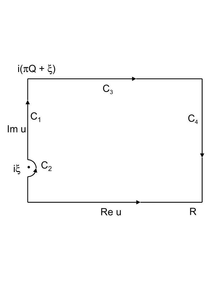
Figure 1: Integration contour chosen for our evaluation of the integral (23).

The continuum limit is then obtained by considering the limiting value of the RHS of Eq.(27) for $Q\rightarrow+\infty$. We now show that the result is the reduced version of Eq.(5) appropriate to the regime $x^{\pm}>0$. Before proceeding we note that $I_{0}(2e^{i\pi/4}\sqrt{u})$ is an analytic function of $u$ throughout the entire finite complex plane since its Taylor series expansion in powers of the argument has an infinite radius of convergence. The remaining factor in the integrand of (27) is analytic throughout the $u$ plane with the exception of simple poles at the discrete set of points $u_{n}=i(2n\pi Q+\xi)$ on the imaginary axis, where $n$ is any integer. In view of these analytic properties of the integrand we can alter the integration contour without changing the value of the integral in (27) as long as we avoid crossing through any of the singular points $u_{n}$ and maintain the given endpoints. The simplest choice of a preferable contour is presented in Fig.1. It consists of the straight-line segments $(C_{1})$ on the imaginary axis, the semi-circle $(C_{2})$ centered on the pole $u_{0}$, the line $(C_{3})$ parallel to the positive real axis, and finally the straight-line segment $(C_{4})$ parallel to the imaginary axis. Note that on $C_{4}$ we have ${\rm Re}~{}u=R$ and we will require that $R/Q>\alpha Q$ where $\alpha>2$.

On the contour $C_{1}$ we have $u=iv$, where $v$ is positive real. One immediately finds that this contribution to $\hat{D}(x)$ may be written as

$$\frac{1}{8\pi Q}P\int\limits_{0}^{\pi Q+\xi}dvJ_{0}(2\sqrt{v})\cot\big{(}(v-\xi)/(2Q)\big{)}-\frac{i}{8\pi Q}\int\limits_{0}^{\pi Q+\xi}dvJ_{0}(2\sqrt{v}),$$ (28)

where $P$ denotes principal value. Each of the two integrals is real and finite. The second term can be evaluated in closed form and the result is

$$-\frac{i}{8\pi}\frac{\sqrt{\pi Q+\xi}}{Q}J_{1}(2\sqrt{\pi Q+\xi}),$$ (29)

and in particular it vanishes in the large $Q$ limit.

In order to obtain the $L\rightarrow\infty$ limiting behavior of the first term of (28), one can replace the cotangent function by the inverse of its argument, so that after the change of variable $v=w^{2}/4$ one obtains

$$P\frac{1}{4\pi}\int\limits_{0}^{\infty}dv\frac{J_{0}(2\sqrt{v})}{v-\xi}=P\frac{1}{2\pi}\int\limits_{0}^{\infty}dw\frac{wJ_{0}(w)}{w^{2}-4\xi}=-\frac{1}{4}N_{0}(2\sqrt{\xi}).$$ (30)

On the infinitesimal semicircle $C_{2}$ defined by $u-i\xi=\epsilon e^{i\theta},-\pi/2\leq\theta\leq\pi/2$, with $\epsilon\rightarrow 0^{+}$, we may use the approximation

$$\frac{1}{\exp\Big{(}\frac{1}{Q}(u-i\xi)\Big{)}-1}\approx\frac{Q}{\epsilon e^{i\theta}}.$$ (31)

Replacing further the function $I_{0}$ by its value at $u_{0}$ and using the relation [11] $I_{0}(2i\sqrt{\xi})=J_{0}(2\sqrt{\xi})$, we find that this contribution to $\hat{D}$ is equal to $\frac{i}{16\pi}J_{0}(2\sqrt{\xi})$. Note that this quantity is independent of $L$ and thus survives in the large-$Q$ limit.

On the horizontal semi-infinite line $C_{3}$ we may write $u=i\xi+Q(i\pi+v)$, where $v$ is real, positive. The contribution to $\hat{D}(x)$ is given by

$$-\frac{1}{4\pi}\int\limits_{0}^{\alpha Q}dv\frac{1}{e^{v}+1}J_{0}\big{(}2\sqrt{\xi+\pi Q-iQv}\big{)}.$$ (32)

The asymptotic analysis of Eq.(32) in the limit $Q\rightarrow+\infty$ is very lengthy and involves substitution of an integral representation of $J_{0}$ combined with the method of steepest descent. The details of this calculation will be given elsewhere [12]. The final result is that the leading behavior of the expression (32) is given by a term proportional to $\exp(iQ)$. This vanishes in the limit $L\rightarrow\infty$ as long as for any finite $L$ the quantity $x^{+}$ includes a small positive imaginary part such that $L\times{\rm Im}(x^{+})\rightarrow\infty$. This requirement is satisfied for example by the choice Im$(x^{+})=O(L^{-1/2})$.

Finally, points on the line segment $C_{4}$ are described by $u=R+iv$, where $v$ is real, positive. The contribution to $\hat{D}(x)$ from $C_{4}$ is then found to be dominated by $\exp\Big{[}-\big{(}\alpha-\sqrt{2\alpha}\big{)}Q\Big{]}$ and thus vanishes in the large-$Q$ limit since we choose $\alpha>2$.

Combining these results we have

$$\lim_{Q\rightarrow\infty}\hat{D}(x^{+}>0,x^{-}>0)=-\frac{1}{4}\Big{(}N_{0}(\mu\sqrt{x^{2}})-iJ_{0}(\mu\sqrt{x^{2}})\Big{)},$$ (33)

in agreement with Eq.(5).

It is easy to see from the formula (23) that results for finite $L$ for the case $x^{+}<0,x^{-}<0$ ($\xi>0,Q<0)$ can be obtained from those for $x^{+}>0,x^{-}>0$ by complex conjugation:

$$F_{1}(e^{-i\xi/|Q|},-i|Q|)=\big{[}F_{1}(e^{i\xi/Q},iQ)\big{]}^{*}.$$ (34)

Likewise, we have for $x^{+}>0,x^{-}<0$ ($Q>0,\xi<0$)

$$\hat{D}(x)=\frac{1}{4\pi}F_{1}(e^{-i|\xi|/Q},iQ),$$ (35)

and this can be used to generate the results also for the regime $x^{+}<0,x^{-}>0$ $(\xi<0,Q<0)$ according to

$$\hat{D}(x)=\frac{1}{4\pi}F_{1}(e^{i|\xi|/|Q|},-i|Q|)=\big{[}\frac{1}{4\pi}F_{1}(e^{-i|\xi|/Q},iQ)\big{]}^{*}.$$ (36)

The evaluation of $F_{1}$ in Eq.(35) for large $L$ proceeds as above using the same multi-component contour except that the semicircle $C_{2}$ is not applicable since the pole $u_{0}$ is situated at $-i|\xi|$. The final result is

$$\lim_{Q\rightarrow+\infty}\hat{D}(x^{+}>0,x^{-}<0)=\frac{1}{4\pi}\int\limits_{0}^{\infty}dv\frac{J_{0}(2\sqrt{v})}{v+\xi}=\frac{1}{2\pi}K_{0}(2\sqrt{|\xi|}),$$ (37)

in agreement with the continuum formula (5). In particular, this result means that since the imaginary part of the function $\hat{D}(x)$ vanishes for spacelike $x^{2}$, the causality is restored in the infinite-volume limit. For large $L$ the leading $L$-dependent terms are of the order $L^{-1/4}$.

Finally we briefly discuss the correlation functions $\hat{S}_{22}$ and $\hat{S}_{11}$ of (18). The first of these is a special case of the function

$$F_{0}(z,q)=\sum_{n=1}^{\infty}{z^{n}}e^{q/n}=\frac{z}{1-z}+q\int\limits_{0}^{\infty}du\frac{1}{z^{-1}e^{u}-1}\frac{I_{1}(2\sqrt{qu})}{\sqrt{qu}},$$ (38)

while $\hat{S}_{11}$ is a special case of

$$F_{2}(z,q)=\sum_{n=1}^{\infty}\frac{z^{n}}{n^{2}}e^{q/n}=\int\limits_{0}^{\infty}du\frac{u}{z^{-1}e^{u}-1}\frac{I_{1}(2\sqrt{qu})}{\sqrt{qu}}.$$ (39)

In the regime $x^{\pm}>0$ we find that

$$\lim_{Q\rightarrow+\infty}\hat{S}_{22}(x) = 4e^{i\frac{\pi}{4}}P\int\limits_{0}^{\infty}dw\frac{J_{1}(w)}{w^{2}-4\xi}-\frac{\pi}{\sqrt{\xi}}e^{-i\frac{\pi}{4}}J_{1}(2\sqrt{\xi})$$ (40)

$$= -\frac{m}{4}\sqrt{\frac{x^{+}}{x^{-}}}\Big{(}J_{1}(m\sqrt{x^{2}})+iN_{1}(m\sqrt{x^{2}})\Big{)}.$$

Likewise, in the same regime, we have

$$\lim_{Q\rightarrow+\infty}\hat{S}_{11}(x)=-\frac{2\pi^{2}}{m}\sqrt{\frac{x^{-}}{x^{+}}}\Big{(}J_{1}(m\sqrt{x^{2}})+iN_{1}(m\sqrt{x^{2}})\Big{)}.$$ (41)

These results are in agreement with the continuum formulas (15).

4 Numerical results

In principle, one may try to evaluate the integral (23) representing the Pauli-Jordan function in finite volume numerically for increasing values of $L$ to examine the rate of convergence towards the continuum result. In practice, this is rather difficult to achieve since the integrand of the representation (23) oscillates rapidly due to the presence of the Bessel function $I_{0}$. Already for relatively small values of $Q$ the amplitudes of these oscillations are so large and the spacings of successive zeros are so small that it is very difficult to reliably evaluate the integral by standard numerical routines. Since it is not our goal to perform extensive numerical analyses in the present work, we have computed the integral for a few relatively small values of $Q(=4,15,18)$ using an integration method based on Chebyshev polynomials as well as by a Clenshaw-Curtis method. For definiteness we set $\mu^{2}x^{+}=1$ so that the corresponding box lengths given by $L=4\pi Q$ are approximately $L=50,188$ and $226$. The results are displayed in Fig.2. An essential difference in the behavior of the Pauli-Jordan commutator function between the space-like region (negative values of $x^{-}/L$) and time-like region (positive $x^{-}/L$) is obvious already for the smallest value $Q=4$. It is also evident that for larger Q the oscillatory behavior of the continuum curve in the time-like region is resolved with increased accuracy. This is particularly true in the interval $0<x^{-}/L<0.5$ but the number and position of oscillations is semiquantitatively reproduced also for $x^{-}/L>0.5$. Although the Pauli-Jordan function for finite volumes is not zero in the space-like region, it is reasonably close to it. We recall that for our choice of $Q$ values we are still very far from the infinite-volume limit so the obtained behavior of the Pauli-Jordan function is very plausible and consistent with our analytical results.

5 Discussion

The Discretized Light Cone Quantization method has led to many interesting results over the last fifteen years. It is however essential that the method satisfy all requirements and principles of a consistent relativistic theory. It is rather clear that restricting a system to a finite spatial volume and imposing (anti)periodic boundary conditions on quantum fields will generally lead to a theory which does not have exactly the same properties as the continuum (infinite-volume) theory. Some finite-volume effects may be present [13]. However, the crucial point is that the continuum limit of a finite-volume theory should recover all necessary properties including e.g. Poincaré symmetry. The principle of microcausality (or locality) is one of the fundamental properties of relativistic dynamics and the DLCQ method would face a serious difficulty if it would be in conflict with this principle. We have demonstrated in the present work analytically as well as numerically that this is not the case. With the infinite number of field modes the violation of microcausality in a LF finite volume with periodic scalar field is only a marginal effect and continuum results including the causal behavior are restored in the $L\rightarrow\infty$ limit. In practice, the DLCQ calculations of mass spectra and wavefunctions are always performed for finite $L$ and with a finite number of Fouriér modes. At this step, the causality may seem to be violated [7] (see also [8] for a treatment that averages over some range of $L$ values and restores the causal behavior in a finite volume). However, as physical quantities calculated with the DLCQ method have to be extrapolated to the continuum limit, there is no inconsistency, since, as we have shown, the causality is restored there.

Our conclusion has been obtained by means of a well defined mathematical treatment leading to an integral representation of the infinite series representing the two-point functions for a finite volume. We have extracted the $L$-independent part of the integral as well as the leading large-$L$ corrections. Our results for the PJ function $2{\rm Im}\hat{D}(x)$ are consistent with the results of Ref.[9]. The method used enabled us however to calculate the complete Wightman functions of two-dimensional free massive bosons and fermions quantized in a finite volume. A detailed discussion of our mathematical treatment will be published separately [12].

Ames Laboratory is operated for the United States Department of Energy by Iowa State University under Contract No. W-7405-Eng-82. One of the authors (L.M.) was partially supported by the Slovak Grant Agency, VEGA Grant No.2/3106/2003.

6 Acknowledgements

The authors would like to thank J. P. Vary for support and Peter Markoš for assistence with the numerical calculations.

Figure 2: The commutator function ${\rm Im}D(x^{+},x^{-})$ evaluated numerically is plotted for three values of $Q$ as a function of $s=x^{-}/L$ and compared with the continuum function $1/4J_{0}(\sqrt{Ls})$ (solid line) in the box of the length $L=4\pi Q$. For simplicity, we chose $\mu^{2}x^{+}=1$. The time-like region corresponds to positive values of $s$, the space-like region to negative ones.

References

- [1] P.A.M. Dirac, Rev. Mod. Phys. 21 (1949) 392.
- [2] H. Leutwyler, J. R. Klauder and L. Streit, Nuovo Cim. 66A (1970) 536.
- [3] F. Rohrlich, Acta Phys. Austriaca 32 (1970) 87.
- [4] T. Maskawa and K. Yamawaki, Prog. Theor. Phys. 56 (1976) 270.
- [5] H.C. Pauli and S.J. Brodsky, Phys. Rev. D 32 (1985) 1993.
- [6] P. Steinhardt, Ann. Phys. 128 (1980) 425.
- [7] Th. Heinzl, H. Kroger and N. Scheu, hep-th/9908173.
- [8] D. Chakrabarti, A. Mukherjee, R. Kundu and A. Harindranath, Phys. Lett. B 480 (2000) 409.
- [9] S. Salmons, P. Grangé and E. Werner, Phys. Rev. D 60 (1999) 067701.
- [10] L. Lewin, Polylogarithms and Associated Functions, North Holland, New York, 1981.
- [11] I. S. Gradhsteyn and I. M. Ryzhik, Tables of Integrals, Series and Products, Alan Jeffrey, Editor, Fifth Ed., Academic Press, New York, 1994.
- [12] L. Martinovic and M. Luban, manuscript in preparation.
- [13] R. Haag, Infinite systems, in: Brandeis Lectures (1971).