Zeta Functions in Brane World Cosmology

Abstract

We present a calculation of the zeta function and of the functional determinant for a Laplace-type differential operator, corresponding to a scalar field in a higher dimensional de Sitter brane background, which consists of a higher dimensional anti-de Sitter bulk spacetime bounded by a de Sitter section, representing a brane. Contrary to the existing examples, which all make use of conformal transformations, we evaluate the zeta function working directly with the higher dimensional wave operator. We also consider a generic mass term and coupling to curvature, generalizing previous results. The massless, conformally coupled case is obtained as a limit of the general result and compared with known calculations. In the limit of large anti-de Sitter radius, the zeta determinant for the ball is recovered in perfect agreement with known expressions, providing an interesting check of our result and an alternative way of obtaining the ball determinant.

YITP-04-59

I Introduction

The idea of living on a membrane embedded in a higher-dimensional spacetime has attracted enormous attention over the past few years, the main motivation being the fact that the localization of particles on branes provides an alternative to the standard picture of Kaluza-Klein compactification rubakov ; akama .

A popular example is the Randall-Sundrum model RS1 , which considers a five-dimensional slice of Anti-de Sitter (AdS) spacetime with the extra dimension compactified to an orbifold having two 3-branes of opposite tension located at its fixed points. This results in a non-factorizable spacetime, which, as Randall and Sundrum have shown, has the important consequence that the effective four-dimensional scale on the negative-tension brane turns out to be exponentially suppressed relative to the higher-dimensional scale. This was originally proposed as a solution to the hierarchy problem by explaining the very small ratio (large hierarchy) of some 17 orders of magnitude between the electroweak scale and the Planck scale observed on our brane, identified as that with negative tension. In this model, the hierarchy arises as a geometrical effect, with gravity being strongly localized around the positive-tension brane.

Pushing this idea further, Randall and Sundrum RS2 showed that the negative-tension brane may actually be absent and the extra dimension possibly infinite in size. In that case, we live on the positive-tension brane with gravity confined around it, recovering its standard Einstein form from an effective four-dimensional point of view. This result does not solve the hierarchy problem, but has stimulated the construction of many new cosmological models. Here we concentrate our attention on the de Sitter brane model, relevant in the construction of brane world models of inflation.

The problem of studying quantum effects in such scenarios is, then, naturally posed. It is immediately clear that when a quantum field is considered on such background spacetimes, quantum effects may play a significant role, the simple contribution that they give to the brane and bulk cosmological constants being an evident example.

A number of people, inspired by previous work in Kaluza-Klein theories tomsplb ; cw , have investigated the possibility that quantum effects from bulk fields could play a role in the consistency of such models by providing a sensible mechanism of stabilization in the Randall-Sundrum two-brane model and in some higher-dimensional generalizations. Various authors have dealt with the problem of quantum effects in brane models and some references are GR ; T ; BR ; GPT ; FT ; FMT1 ; FMT2 ; SS ; MN ; KT . The lowest order quantum corrections arising from bulk fields on the Randall-Sundrum background have been calculated in a variety of ways, and then extended to some general classes of higher-dimensional spacetimes in Refs. FGPT ; FP ; Fl . Ref. GP considers the case of scalar and gauge fields in the Randall Sundrum model and interprets the result in terms of the AdS/CFT correspondence, showing explicitly that quantum effects could provide a sensible stabilization mechanism.

It is worth mentioning that in most of the previous work, the geometry of the branes was assumed to be flat, which greatly simplifies the study of quantum effects. When the branes are curved, as happens, for example, in de Sitter or hyperbolic brane models, and where the Casimir energy could have some effect on the cosmological evolution of the brane, the situation becomes more complicated.

Some work in this direction has been carried out in Refs. NOZ ; NS ; ENOO ; MNSS . Specifically, in Refs. NOZ ; NS , the vacuum energy for a massless conformally coupled scalar field in a brane world corresponding to de Sitter branes in an AdS bulk has been evaluated. This calculation, which is technically the simplest, is carried out by working in a conformally related spacetime, similar in form to the Einstein universe. Zeta function regularization is employed and the result shows that the vacuum energy is zero for the one brane configuration. These results have been extended to the case of conformally coupled Majorana spinors in Ref. MNSS , still by making use of conformal transformations. The cases of a massless conformally coupled scalar field and of a massive minimally coupled field for de Sitter branes embedded in both de Sitter and AdS bulks have been considered in Ref. ENOO , where the vacuum energy is computed once again by using conformal and zeta regularization techniques and is found to be zero for the one brane case. Refs. NOZ ; Norm consider a somewhat related set-up and compute the effective action for scalar fields in an AdS bulk bounded by AdS branes, still by making use of conformal transformations.

Apart from the relatively simple case of massless, conformally coupled field, the general case has not yet been studied. The present paper is devoted to providing a new derivation of the zeta function and of the functional determinant for a scalar field in a de Sitter brane model. The method is very general and applies, in principle, to a number of situations, where the methods based on conformal transformations or dimensional reduction cannot be applied at ease.

We perform the calculation by directly working in the higher-dimensional spacetime and evaluate the zeta function for the original higher-dimensional wave operator. With respect to the previously studied cases, we have to deal with two main problems. The first is to compute a zeta function where the operator spectrum is not known, for which we adopt the technique developed in Refs. IGM ; BKK ; BKKM ; KM ; BEK ; BKD ; Klausbook . This general technique, elaborated in various forms, allows one to obtain the zeta function using only the knowledge of the basis functions. Such a method is applicable whenever an implicit equation satisfied by the eigenvalues is known, and has already been applied in the context of brane models. We stress, however, that in the case of flat branes the basis functions can be conveniently expressed in terms of Bessel functions, which greatly simplifies the calculation. The second main problem is that, for the class of spacetimes we consider, namely an AdS bulk bounded by a de Sitter brane, the basis functions are expressed as a combination of generalized Legendre functions, which are considerably less manageable. However, the method developed in Ref. BKK proves to be particularly useful and we closely follow their approach in our calculation.

The structure of the paper is as follows. In the next section, we discuss the spacetime configuration of the de Sitter brane model and solve the higher-dimensional scalar wave equation on such a background spacetime. For the sake of generality, we consider a massive scalar field coupled to the higher-dimensional curvature. In the subsequent section, after having described the general technique of Ref. BKK , we pass to the main task at hand, which is the evaluation of the zeta function for a de Sitter brane model. After having obtained the general result, we consider two limiting cases, which provide a non trivial check on the method used as well as the actual calculation. First we specify the result to the conformally coupled case and compare with that of Refs. NOZ ; NS ; ENOO ; MNSS . Then we consider the limit of large AdS curvature radius $\ell$, which should reproduce a ball-like geometry. The last section is left for conclusions. Several technical results regarding the asymptotic expansion of the generalized Legendre functions, as well as the derivations of certain results used in the calculation, are reported in the appendices.

II Scalar fields on de Sitter brane backgrounds

The background configuration we consider is described by the action

$$S=\int d^{5}x\sqrt{-g^{(5)}}\left({1\over 2\kappa^{2}}({\cal R}-2\Lambda_{5})\right)-\int d^{4}x\sqrt{-g^{(4)}}~{}\tau~{},$$ (1)

where

$$\Lambda_{5}=-{6\over\ell^{2}}$$ (2)

is a higher-dimensional, negative, bulk cosmological constant term, $\tau$ is the brane tension and $\kappa^{2}$ is proportional to the five dimensional gravitational constant. The corresponding solution of the setup, with the usual cosmological symmetries, has an AdS five-dimensional geometry; $\ell$ is the radius of the five dimensional AdS space.

A convenient scaling of the time coordinate allows one to write the metric as

$$ds^{2}=dr^{2}+(H\ell)^{2}\sinh^{2}(r/\ell)[-dt^{2}+H^{-2}e^{2Ht}d{\bf x}^{2}_{3}]~{},$$ (3)

where the coordinate $r$ parameterizes the extra dimension and the time coordinate corresponds to the cosmic time parameter on the brane. For notational convenience, we define

$$a(r)=H\ell\sinh(r/\ell).$$ (4)

A ${\mathbb{Z}}_{2}$-symmetric brane world can then be constructed in a standard way by taking two slices of the space and gluing them along the brane located at $r_{0}$. In such a case, the junction conditions at the brane give the Friedmann equation

$$H^{2}={\Lambda_{5}\over 6}+\left({\kappa^{2}\over 6}\right)^{2}\tau^{2}~{}.$$ (5)

In the present case, the Hubble parameter, $H$, is constant, so that the brane geometry is de Sitter. The Hubble parameter is related to the brane position $r_{0}$ according to

$$H^{2}={1\over\ell^{2}\sinh^{2}(r_{0}/\ell)}~{}.$$ (6)

On such a background, we consider a bulk scalar field and ignore its back reaction. It satisfies the Klein-Gordon equation

$$(-\Box_{\rm E}+m^{2}+\xi{\cal R})~{}\varphi(x,r)=0~{}.$$ (7)

For the sake of generality, we consider the brane to be $D$- rather than four-dimensional, for the remainder of the present section. Furthermore, for later convenience, we transform to Riemannian signature. Hence, $\Box_{\rm E}$ is the $(D+1)$-dimensional d’Alembertian on Riemannian space and ${\cal R}$ is the scalar curvature, given by

$${\cal R} = a^{-2}(r)~{}{\cal R}_{\Sigma}-\left[2D{a^{\prime\prime}(r)\over a(r)}+D(D-1)\left({a^{\prime}(r)\over a(r)}\right)^{2}\right]~{},$$ (8)

where ${\cal R}_{\Sigma}=D(D-1)H^{2}$ is the scalar curvature of the de Sitter brane, which is a $D-$sphere of radius $H^{-1}$.

We are interested in finding the eigenmodes $\varphi_{n,j}(x,r)$ and eigenvalues $\lambda_{n,j}^{2}$ of the above field operator, defined by

$$(-\Box_{\rm E}+m^{2}+\xi{\cal R})~{}\varphi_{n,j}(x,r)={\lambda_{n,j}^{2}}~{}\varphi_{n,j}(x,r)~{}.$$ (9)

Let us assume that the modes are separable in the variables $x$ and $r$:

$$\varphi_{n,j}(x,r)=\phi_{j}(x)f_{n,j}(r),$$ (10)

where the spherical eigenfunctions satisfy

$$-\Box_{\Sigma}\phi_{j}(x)=j\left(j+D-1\right)H^{2}\phi_{j}(x),$$ (11)

where $\Box_{\Sigma}$ is the d’Alembertian on the de Sitter section and $d_{j}$ the degeneracy factor,

$$d_{j}=(2j+D-1){(j+D-2)!\over j!(D-1)!}$$ (12)

with $j=0,1,2,\dots$. Using Eq. (11) in Eq. (9) allows us to find the equation of motion for the radial eigenfunctions:

$$\left[-a^{-D}(\partial_{r}a^{D}\partial_{r})+a^{-2}j\left(j+D-1\right)H^{2}+m^{2}+\xi{\cal R}\right]f_{n,j}(r)=\lambda_{n,j}^{2}~{}f_{n,j}(r)~{},$$ (13)

whose solution can be written in terms of toroidal Legendre functions

$$f_{n,j}(\eta)=(H\ell)^{1/2-D/2}\sinh^{1/2-D/2}(\eta)\left[A_{n,j}P_{i\omega_{n,j}-1/2}^{-\nu_{j}}(\cosh\eta)+B_{n,j}Q_{i\omega_{n,j}-1/2}^{-\nu_{j}}(\cosh\eta)\right]~{},$$ (14)

where we have defined $\eta=r/\ell$. The order and degree of the associated Legendre functions are

$$\nu_{j}=\left(j+{D-1\over 2}\right)\qquad\mbox{and}\qquad\omega_{n,j}=\sqrt{\ell^{2}\lambda^{2}_{n,j}-\sigma^{2}}~{},$$ (15)

where

$$\sigma^{2}=\ell^{2}m^{2}+\xi\ell^{2}{\cal R}+D^{2}/4~{}.$$ (16)

Regularity at the origin implies that $B_{n,j}=0$, as follows from examining the small-argument behavior of the generalized Legendre functions.

Thus, our eigenfunctions take the form

$$f_{n,j}(\eta)=A_{n,j}a^{\frac{1-D}{2}}(\eta)~{}P_{i\omega_{n,j}-1/2}^{-\nu_{j}}(\cosh\eta),$$ (17)

with $a(\eta)=H\ell\sinh\eta$.

As well as the solution in the bulk, we must also consider the boundary condition on the brane, which can be obtained by integrating (13) across the brane. In general, the ${\mathbb{Z}}_{2}$ symmetry allows us to choose either an untwisted field configuration, such that $f(\eta)=f(-\eta)$, corresponding to Robin boundary conditions

$$\partial_{\eta}f_{n,j}(\eta_{0})=-{2D\xi\over\ell}\coth(\eta_{0})f_{n,j}(\eta_{0})~{},$$ (18)

or alternatively a twisted field configuration, such that $f(\eta)=-f(-\eta)$, corresponding to Dirichlet boundary conditions

$$f_{n,j}(\eta_{0})=0~{}.$$ (19)

In the remainder of the paper we focus our attention to Dirichlet boundary conditions.

III Zeta function for de Sitter brane models

III.1 General method

The main scope of this paper is to compute the zeta function and the functional determinant for a bulk scalar field on a de Sitter brane background. For calculational simplicity, we take a field obeying Dirichlet boundary conditions, although the method can be applied to more general situations with few calculational modifications. To deal with the case of de Sitter brane models, we follow the approach of Refs. IGM ; BKK ; BEK ; BKD ; Klausbook , where a calculational technique for $\zeta$-functions of differential operators on manifolds with boundaries with explicitly unknown spectra has been developed and applied (see Refs. BKK ; BKKM ; KM ) to evaluate the one-loop contribution from the graviton, and matter fields, to the Hartle-Hawking wave function. Here we summarize their method.

It is a well-known fact that the one-loop effective action can be written as

$$\Gamma^{(1)}={1\over 2}~{}\mbox{Tr}\ln{\Delta}~{},$$ (20)

where $\Delta$ is a second-order differential operator, in our case given by

$$\Delta=-\Box_{E}+m^{2}+\xi{\cal R}~{}.$$ (21)

$\Gamma^{(1)}$ can be expressed in terms of a generalized $\zeta$-function

$$\zeta(s)=\sum_{\lambda}\lambda^{-s}~{},$$ (22)

with $\lambda$ being the eigenvalues of the operator $\Delta$, which we assume to be positive definite. One has

$$\Gamma^{(1)}=-{1\over 2}\zeta^{\prime}(0)-{1\over 2}\zeta(0)\ln\mu^{2}~{},$$ (23)

where $\mu$ is the renormalization scale. Thus, we see that the main problem is reduced to that of evaluating the $\zeta$-function and its derivative at $s=0$.

Usually, the computation of the $\zeta$-function requires explicit knowledge of the spectrum. However, in many situations of interest, the eigenvalues are not explicitly known. To bypass this kind of problem, various authors have developed a calculational technique that allows one to evaluate the $\zeta$-function and related quantities like functional determinants, Casimir energies and effective actions, when such information on the eigenvalues is lacking and the only knowledge of the spectrum is via an implicit equation BKK ; BEK ; BKD ; Klausbook . Generally, one considers the eigenvalue problem associated with the operator $\Delta$:

$$\Delta u_{\nu}(x)=\lambda u_{\nu}(x)~{},$$ (24)

where the parameter $\nu$ enumerates the independent solutions of (24). A degeneracy factor $d(\nu)$ is associated with each $\nu$. Imposing the relevant boundary conditions leads to an equation of the form

$$F(\lambda,\nu)=0~{},$$ (25)

where the function $F(\lambda,\nu)$ depends on the mode functions, the eigenvalues $\lambda$, the index $\nu$ and eventually other parameters inessential for the present discussion.

To evaluate the $\zeta$-function it is not necessary to solve the previous equation, as is clear by making use of the residue theorem, which allows one to write

$$\zeta(s)={1\over 2\pi i}\int_{\cal C}\omega^{-s}{d\over d\omega}\sum_{\nu}d(\nu)\ln F(\omega,\nu)d\omega~{},$$ (26)

where the contour $\cal C$ is chosen to enclose all the positive solutions of (25) in the complex $\omega-$plane.

For the explicit calculation, it is convenient to express this contour integral as an integral along the real line, which can be achieved by appropriately deforming the contour ${\cal C}$. Typically, if the function $F(\omega,\nu)$ satisfies certain properties, as in the case we will consider in the next section, a choice of a contour like the one in Fig. 1, allows one to rewrite the integral (26) as

$$\zeta(s)={\sin\pi s\over\pi}\int_{0}^{\infty}z^{-s}{d\over dz}\sum_{\nu}d(\nu)\ln F(z,\nu)dz~{}.$$ (27)

The source of divergences in the above expression come from the large $\nu$ behavior and the integration over $z$. We need to check that large values of $s$ indeed regulate $\zeta(s)$. Let us first presuppose that this is possible and, assuming $s$ to be large enough, we swap the order of integration and summation and consider the asymptotic behavior of the integral

$$\int_{0}^{\infty}z^{-s}{d\over dz}\ln F(z,\nu)dz~{}$$ (28)

for $\nu\rightarrow\infty$ and its integrand for $z\rightarrow\infty$ and $z\rightarrow 0$. Now, it is possible to obtain a uniform asymptotic expansion $\Phi(\nu,z/\nu)$ of $\ln F(z,\nu)$ such that $\nu\rightarrow\infty$, while the ratio $z/\nu$ is held fixed. Thus

$$\ln F(z,\nu)\sim\Phi(\nu,z/\nu)~{},$$ (29)

for large $\nu$. There are two important features of this expansion, aside from its uniformity: it has a power-law behavior of fixed order in $\nu$, as we shall illustrate for our case, and it is valid in the full range of the ratio $0\leq z/\nu<\infty$. If the integral (28) is finite for a large enough value of $s$, which is true in our case, then uniformity, together with these two properties ensures the convergence of the sum over (28), for sufficiently large $s$. This can be proved under quite general assumptions, but here we content ourselves with showing that this is true for the case under study. Finally, a simple rescaling allows us to write

$$\zeta(s)={\sin\pi s\over\pi}\sum_{\nu}d(\nu)\nu^{-s}\int_{0}^{\infty}z^{-s}{d\over dz}\Phi(z,\nu)dz~{}.$$ (30)

This verifies that it is possible to regularize the divergences by a suitable choice of $s$. We now interchange the integration and summation back to their original order and write

$$\zeta(s)={\sin\pi s\over\pi}\int_{0}^{\infty}z^{-s}{d\over dz}I(z,s)dz~{},$$ (31)

where $I(z,s)$ is given by

$$I(z,s)=\sum_{\nu}d(\nu)\nu^{-s}{d\over dz}\ln F(z,\nu)~{}.$$ (32)

In order to further proceed with the evaluation of the $\zeta$-function, we must analytically continue to $s=0$. We expand the sum (32) around small values of $s$, which generally develops a pole:

$$I(z,s)\sim{I^{\rm pole}(z)\over s}+I^{\rm R}(z)+O(s)~{}.$$ (33)

It is now possible to use the following lemma along with the properties of the asymptotic expansion to compute $\zeta(s)$. Consider a function ${\it f}(x)$ which is analytic at $x=\epsilon$, for some small $\epsilon$, and has the following general asymptotic behavior, when $x\rightarrow\infty$,

$${\it f}(x)=\sum_{k=1}^{\rho_{k}<N}\left({\it f}_{k}+\bar{\it f}_{k}\ln x\right)x^{\rho_{k}}+[{\it f}]_{\rm log}\ln x+[{\it f}]_{\rm reg}+O(x^{-1})~{},\qquad\rho_{k}>0~{},$$ (34)

where the subscripts ${\rm log}$ and ${\rm reg}$ refer to the solely logarithmic and regular (non-singular) parts of ${\it f}(x)$ in the large $x$ limit. Then, there exists the analytic continuation of the integral

$$\int_{\epsilon}^{\infty}{dx\over x^{s}}{d\over dx}{\it f}(x)={[{\it f}]_{\rm log}\over s}+[{\it f}]^{\infty}_{\epsilon}+O(s)~{},$$ (35)

where $[{\it f}]^{\infty}_{\epsilon}\equiv[{\it f}]_{\rm reg}-{\it f}(\epsilon)$, for example see Ref. BKK .

On the basis of the uniform asymptotic expansion of the eigenfunctions, it is possible to prove that $I^{\rm pole}(z)$ and $I^{\rm R}(z)$ behave as (34) and we also assume that $[I^{\rm pole}]_{\rm log}=0$, which we shall show to be true in the case of interest to us. It is now a simple matter to apply the result (35) to $I^{\rm pole}(z)$ and $I^{\rm R}(z)$ to get

$$\zeta(s)=[I^{\rm R}]_{\rm log}+[I^{\rm pole}]^{\infty}_{0}+s\left\{[I^{\rm R}]^{\infty}_{0}-\int^{\infty}_{0}dz\ln z^{2}{dI^{\rm pole}(z)\over dz}\right\}+O(s^{2})~{},\qquad s\rightarrow 0~{}.$$ (36)

This equation can then be used to get the value of the $\zeta$-function and its derivative at $s=0$.

III.2 Explicit evaluation of the $\zeta$-function

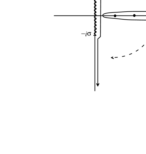
Figure 1: The original contour (enclosing the positive real zeros) and the deformed contour lying along the imaginary axis. The deformed contour $C^{\prime}$ is closed at infinity by a semi-circle of infinite radius.

We now pass to the explicit evaluation of the $\zeta$-function for the scalar field on the de Sitter background, described in section (II). We have seen that, for Dirichlet boundary conditions, the eigenvalues are given by the solution of the implicit equation

$$F(\omega_{n,j};\nu_{j})\equiv 2^{\nu_{j}}\Gamma(1+\nu_{j})P_{i\omega_{n,j}-1/2}^{-\nu_{j}}(\cosh\eta_{0})=0~{}.$$ (37)

Note that we have multiplied the Legendre function by the factor $2^{\nu_{j}}\Gamma(1+\nu_{j})$ as this does not change the solution of the eigenvalue equation (19) and, on the other hand, produces some simplifications in the calculations at a later stage. It is also clear that any factor independent of $z$ does not affect the contour integral (26).

Thus the $\zeta$-function can be expressed by the double sum

$$\zeta(s)=\sum_{n,j}d_{j}~{}\lambda_{n,j}^{-2s}=\ell^{2s}\sum_{n,j}d_{j}~{}\big{(}\omega^{2}_{n,j}+\sigma^{2}\big{)}^{-s},$$ (38)

with $\omega_{n,j}$ defined in (15) being the solutions to (37). As described in the previous subsection, we can use the residue theorem to express the $\zeta$-function as a contour integral, in terms of the complex parameter $\omega$

$$\zeta(s)={\ell^{2s}\over 2\pi i}\sum_{j}d_{j}\int_{\cal C}{d\omega\over~{}(\omega^{2}+\sigma^{2})^{s}}{d\over d\omega}~{}\ln F(\omega,\nu_{j})~{},$$ (39)

where the contour ${\cal C}$ is chosen to enclose the real positive zeros of $F(\omega,\nu_{j})$.

By appropriately deforming the contour (see Fig. 1) and by performing some formal manipulations, we arrive at

$$\zeta(s)={\sin\pi s\over\pi}\int^{\infty}_{0}{dz^{2}\over z^{2s}}{d\over dz^{2}}~{}I(z^{2},s)~{},$$ (40)

where

$$I(z^{2},s)=\sum_{j}d_{j}{1\over\nu_{j}^{2s}}~{}\ln[~{}2^{\nu_{j}}\Gamma(1+\nu_{j})~{}P^{-\nu_{j}}_{\sqrt{\nu_{j}^{2}z^{2}\ell^{2}+\sigma^{2}}-\frac{1}{2}}(\cosh\eta_{0})]~{}.$$ (41)

As in the previous subsection, we split the contributions to the $\zeta-$function into one regular plus one polar piece:

$$\zeta(s)=\zeta_{R}(s)+\zeta_{P}(s)~{},$$ (42)

where

$$\zeta_{R}(s)={\sin\pi s\over\pi}\int_{0}^{\infty}dz^{2}z^{-2s}{d\over dz^{2}}I^{R}(z^{2},s)~{},$$ (43)

and

$$\zeta_{P}(s)={\sin\pi s\over\pi}\int_{0}^{\infty}dz^{2}z^{-2s}{d\over dz^{2}}I^{\rm pole}(z^{2},s)~{}.$$ (44)

In the previous two expressions $R$ means that we have to take the regular part of the large$-z$ expansion of the integrand, whereas $pole$ refers to the pole part at large $z$.

The integrand functions have the asymptotic behavior (34), as shown in Appendix A; we are, therefore, justified in applying the lemma discussed previously. Then, it is easy to see that

$$\zeta_{R}(s)=[I^{R}]_{\rm log}+s([I^{R}]_{\rm reg}-I^{R}(0))+O(s)~{},$$ (45)

and

$$\zeta_{P}(s)=[I^{\rm pole}]_{\rm log}-s\int_{0}^{\infty}dz^{2}\ln z^{2}{dI^{\rm pole}(z^{2})\over dz^{2}}+O(s)~{}.$$ (46)

The derivative can now be calculated easily and the previous results combine to give

$$\zeta(0)=[I^{\rm R}]_{\rm log}+[I^{\rm pole}]_{\rm reg}-I^{\rm pole}(0)~{},$$ (47)

and

$$\zeta^{\prime}(0)=[I^{\rm R}]_{\rm reg}-I^{\rm R}(0)-\int^{\infty}_{0}dz^{2}\ln z^{2}{dI^{\rm pole}(z^{2})\over dz^{2}}~{},$$ (48)

where we have anticipated the fact that $[I^{\rm pole}]_{\rm log}=0$, as shown in Appendix B. The asymptotic expansion of $I(z^{2},s)$ is also given in Appendix B, where the various pieces appearing in (47) and (48) are obtained.

For $\zeta(0)$, $[I^{\rm R}]_{\rm log}$, $[I^{\rm pole}]_{\rm reg}$ and $I^{\rm pole}(0)$ are needed, and Eqs. (68), (71) and (72) provide them. Some algebra leads to the desired result:

$$\zeta(0)={1\over 6}{17\over 1920}+\frac{\sinh^{2}\eta_{0}}{32}\left(1+2\sinh^{2}\eta_{0}\right)\left(\sigma^{2}-1/4\right)-\frac{\,{\sinh^{4}\eta_{0}}}{48}\left(\sigma^{2}-1/4\right)^{2}~{}.$$ (49)

On the other hand, the evaluation of $\zeta^{\prime}(0)$ requires the knowledge of $[I^{\rm R}]_{\rm reg}$, $I^{\rm R}(0)$ and of the integral piece appearing in Eq. (48). These are calculated in Appendix B and the results are reported in formulas (73), (84) and (102), which, combined together, lead to the following expression for $\zeta^{\prime}(0)$:

$$\zeta^{\prime}(0)=\zeta(0)\ln(\ell\sinh\eta_{0})^{2}+\Delta_{1}+\Delta_{2}+\Delta_{3}+\Delta_{4}$$ (50)

where

$$\Delta_{1}\equiv{47\over 9216}-{1\over 64}\zeta^{\prime}(0,1/2)+{1\over 24}\zeta^{\prime}(-1,1/2)+{1\over 24}\zeta^{\prime}(-2,1/2)-{1\over 6}\zeta^{\prime}(-3,1/2)+{1\over 12}\zeta^{\prime}(-4,1/2)$$ (51)

$$\Delta_{2}\equiv-{137\over 7200}\left.{d^{5}\phi\over dx^{5}}\right|_{x=0}+{1\over 120}\int_{0}^{\infty}dx\ln x{d^{6}\phi\over dx^{6}}+\int^{\infty}_{2/3}x^{-6}\phi(x)~{}dx~{},$$ (52)

$$\Delta_{3}\equiv-~{}i\int_{0}^{\infty}dx{(ix+3/2)^{3}/3-(ix+3/2)/12\over e^{2\pi x}-1}~{}\ln[{\cal Z}(ix+3/2)]-{\cal C.C.}-~{}\frac{1}{2}\ln[{\cal Z}(3/2)]~{},$$ (53)

$$\Delta_{4}\equiv-{73\over 1536}\sinh^{2}\eta_{0}-{251\over 3072}\sinh^{4}\eta_{0}+{7\over 64}\sigma^{2}\sinh^{2}\eta_{0}+{31\over 192}\sigma^{2}\sinh^{4}\eta_{0}-{1\over 48}\sigma^{4}\sinh^{4}\eta_{0}~{},$$ (54)

where

$$\phi(x)\equiv{1\over 3}\left(x-{1\over 3}x^{3}\right)\ln{\cal Z}(1/x)~{},$$ (55)

$${\cal Z}(x)\equiv 2^{x}\Gamma(1+x)P^{-x}_{\sigma-1/2}(\cosh\eta_{0})~{}.$$ (56)

Formulas (49) and (50) represent the main result of our paper.

IV Limiting cases

The results obtained in the previous section for the zeta function and its derivative are valid for a scalar field of arbitrary mass $m$ and coupling $\xi$. Here we focus on the specific case of a massless conformally coupled field, as this allows us to compare our result to that of Refs. NS ; MNSS . By setting $\sigma=1/2$ in Eqs. (49) and (50), the following expressions are found:

$$\zeta(0) = {1\over 6}{17\over 1920}~{},$$

$$\zeta^{\prime}(0) = {1\over 6}{17\over 1920}\ln(\ell\sinh\eta_{0})^{2}-{31\over 1536}\sinh^{2}\eta_{0}-{131\over 3072}\sinh^{4}\eta_{0}+\Delta_{1}~{}.$$ (57)

These values can be compared with those of Ref. MNSS . After sorting out some transcription errors in Tables I and II of the mentioned reference, the result is found to disagree by a constant number. The question arises as to whether or not this difference is at all significant. Clearly, this constant difference can be reabsorbed by redefining the renormalization scale, and therefore it does not have any physical significance. However, from the mathematical point of view, the origin of such a difference is not so clear-cut.

This disagreement has led us to consider another limiting case, which is obtained when the AdS curvature radius $\ell$ is large. This should reproduce the ball geometry, and corresponds, in our terminology, to $\ell>>r_{0}$, i.e. $\eta_{0}<<1$. This result has been computed by various authors using different techniques BEK ; BKD ; Klausbook ; BEGK ; Dowker , and therefore it should provide quite a robust check on the result, and also an alternative derivation, although more involved than necessary, of the zeta determinant for the ball. Now, in the limit of $\eta_{0}<<1$, we find

$$\zeta(0) = {1\over 6}{17\over 1920}~{},$$

$$\zeta^{\prime}(0) = {1\over 6}{17\over 1920}\ln r_{0}^{2}+{47\over 9216}-{1\over 64}\zeta^{\prime}(0,1/2)$$

$$+ {1\over 24}\zeta^{\prime}(-1,1/2)+{1\over 24}\zeta^{\prime}(-2,1/2)-{1\over 6}\zeta^{\prime}(-3,1/2)+{1\over 12}\zeta^{\prime}(-4,1/2)~{}.$$

This result is found in full agreement with those of Refs. Klausbook ; BEGK ; Dowker , thus providing a robust check of our result. We note that such a limiting case is not recovered neither by the result of Refs. NS ; MNSS nor by that of Refs. NOZ ; ENOO .

In order to find some explanation for the difference, let us briefly reconsider the method used there. The first step of the method used in Refs. NOZ ; NS ; ENOO ; MNSS is a conformal transformation that changes the original background spacetime into a different one, where the evaluation of the zeta determinant is, in principle, easier. In Refs. NOZ ; NS ; ENOO ; MNSS this corresponds to a coordinate transformation, $dz=dr/a(r)$, upon which the original line element becomes

$$ds^{2}=a^{2}(r)(dz^{2}+ds^{2}_{\Sigma})~{}.$$ (59)

In other words, a conformal rescaling of the metric by $a(r)$ leaves us with a flat cylinder with a de Sitter cross-section. This is the starting point taken in the above mentioned articles. One immediately sees that the coordinate $r$ lies in the range of $0\leq r\leq r_{0}$ in the original frame, whereas in the conformally transformed one $z$ lies between $z(r_{0})\leq z\leq\infty$, implying that the conformally transformed spacetime corresponds to a semi-infinite cylinder and a more important point is that the conformal transformation is well defined at every point of the AdS bulk, except from the center where it breaks down. This observation raises the question as to whether or not this procedure is actually valid. Certainly it requires care. Obviously, in the two brane setup this problem does not exists since $r$ is never $0$.

V Concluding remarks

The present article was devoted to providing an alternative derivation of the zeta function and of the functional determinant for a scalar field on a de Sitter brane background, which consists of a higher dimensional AdS bulk spacetime bounded by a de Sitter section. We considered the general case of a non-zero mass and coupling to the scalar curvature, thus generalizing previous results limited to zero mass and conformal coupling.

For simplicity, we considered the case of a five dimensional bulk spacetime and Dirichlet boundary conditions. However, the result can be extended, with no additional technical problems and modulo some algebra, to other boundary conditions or higher dimensionalities. The choice of five dimensions was also motivated by the possible relevance of our calculation for the bulk inflaton model proposed in KKS ; HS .

One of the interesting points of the approach developed here lies in the fact that we do not make use of conformal transformations as is done in Refs. NOZ ; NS ; MNSS ; ENOO and whose results, in the limit of large AdS radius does not reproduce that of the ball given in Refs. Klausbook ; BEGK ; Dowker

The basic tools of our calculation were a contour integral representation for the zeta function and asymptotics of the eigenfunctions, for which we have followed Refs. BKK ; BKD ; Klausbook . In particular, the method devised in BKK has proven to be very powerful, and extremely useful in the case discussed here.

As a check on the calculation, we have considered the limiting case of massless, conformally coupled fields, which was found to disagree with the result of NS ; MNSS . The difference amounts to a constant, which is physically harmless and can be removed by redefining the renormalization scale. This difference motivated us to consider another limiting case, which is obtained when the curvature radius of the higher dimensional AdS space is very large, leading to a ball-like geometry, for which extensive calculations of the zeta determinant are available Klausbook ; BEGK ; Dowker . In such a limit we recover those results and this should provide a robust check of our calculation, and, interestingly, this limit provides an alternative derivation, although technically unnecessary, of the ball determinant. We note that the results for the derivative of the zeta function given in Refs. NOZ ; NS ; MNSS ; ENOO do not recover this limit.

Various generalizations of the work presented here are possible. Extensions to higher dimensionalities, different boundary conditions, two-brane setups and higher spin fields should follow without additional difficulties and only a larger amount of algebra might be needed. Looking at the possible relevance of these kinds of calculations in the bulk inflaton model and more generically in brane world cosmology also deserves further study. We hope to report on these issues in our future work.

Appendix A Uniform asymptotic expansion of the Legendre functions

Following Refs. Khus and Thorne , the uniform asymptotic expansion of $P^{-\nu}_{\mu-1/2}(\cosh\eta)$ can be obtained. In this appendix, we simply outline the procedure and extend the results to the case of the logarithm of the Legendre function $P_{\mu}^{\nu}(\cosh\eta)$.

For large values of $\mu$, the solution of the Legendre differential equation can be written in the well-known WKB form. When substituted into the original equation, this leads to a set of recursive equations that allow one to determine the expansion. Omitting the details, the result is

$$P_{\mu-1/2}^{\nu}(\cosh\eta)=\sqrt{{t\over 2\pi\nu}}e^{\nu\xi}\mu^{-\nu}+\sum_{i}\alpha_{i}\nu^{-i}~{},$$ (60)

where the functions $t$ and $\xi$ are given by

$$t={1\over\sqrt{1+\tau^{2}\sinh^{2}\eta}}~{},$$ (61)

and

$$\xi=\ln\frac{\tau\sinh\eta}{\sqrt{1+\tau^{2}\sinh^{2}\eta}+\cosh\eta}-\tau\left[\tanh^{-1}{1\over\tau}-\tanh^{-1}{1\over\tau t\cosh\eta}\right]+1~{}.$$ (62)

We have defined $\tau=\mu/\nu$ and the coefficients $\alpha_{i}$ can be computed recursively. They are quite lengthy for increasing values of $i$ and since they are not used directly we do not report them. The interested reader is addressed to the work of Refs. Thorne ; Khus , where they are also derived.

It is a relatively simple task to get the logarithm of the previous expression and this can be achieved by using a symbolic manipulation program. The result is

$$\ln P^{-\nu}_{\mu-1/2}(\cosh\eta)\sim\ln\left[\sqrt{t\over 2\pi\nu}\,e^{\nu\xi}\mu^{-\nu}\right]+\sum_{n=1}^{\infty}{E_{n}(t,\tau)\over\nu^{n}}~{},$$ (63)

where it is essential to note that the coefficients $E_{n}(t,\tau)$ are bounded in the full range $0\leq\tau<\infty$ and for large $\tau$ they scale as inverse powers of $\tau$. For $\nu\rightarrow\infty$ they exhibit a power law growth of finite order in $\nu$. This can be checked for the first four coefficients $E_{n}$, which are found to be

$$E_{1} = -{1\over 24(\tau^{2}-1)}\left(5\tau^{2}t^{3}\cosh^{3}\eta-3t\cosh\eta+1-3\tau^{2}t\cosh\eta\right),$$

$$E_{2} = {1\over 16(\tau^{2}-1)^{2}}\left(-1+t^{2}\cosh^{2}\eta+7\tau^{2}t^{2}\cosh^{2}\eta-\tau^{2}-6\tau^{4}t^{4}\cosh^{4}\eta+\tau^{4}t^{2}\cosh^{2}\eta-6\tau^{2}t^{4}\cosh^{4}\eta\right.$$

$$\left.+5\tau^{4}t^{6}\cosh^{6}\eta\right),$$

$$E_{3} = -{1\over 40320(\tau^{2}-1)^{3}}\left(118881\tau^{4}t^{5}\cosh^{5}\eta-51765\tau^{2}t^{3}\cosh^{3}\eta+18270\tau^{2}t\cosh\eta-51765\tau^{4}t^{3}\cosh^{3}\eta\right.$$

$$\left.+2835\tau^{4}t\cosh\eta+33453\tau^{6}t^{5}\cosh^{5}\eta-2625\tau^{6}t^{3}\cosh^{3}\eta-69615\tau^{6}t^{7}\cosh^{7}\eta+33453\tau^{2}t^{5}\cosh^{5}\eta\right.$$

$$\left.-69615\tau^{4}t^{7}\cosh^{7}\eta+38675\tau^{6}t^{9}\cosh^{9}\eta-98+2835t\cosh\eta-294\tau^{2}-2625t^{3}\cosh^{3}\eta\right),$$

$$E_{4} = {1\over 128(\tau^{2}-1)^{4}}\left(565\tau^{8}t^{12}\cosh^{12}\eta+1503\tau^{4}t^{4}\cosh^{4}\eta-2282\tau^{6}t^{6}\cosh^{6}\eta-288\tau^{4}t^{2}\cosh^{2}\eta\right.$$ (64)

$$\left.-1356\tau^{6}t^{10}\cosh^{10}\eta-288\tau^{2}t^{2}\cosh^{2}\eta+542\tau^{2}t^{4}\cosh^{4}\eta-2282\tau^{4}t^{6}\cosh^{6}\eta+542\tau^{6}t^{4}\cosh^{4}\eta\right.$$

$$\left.-18\tau^{6}t^{2}\cosh^{2}\eta-284\tau^{2}t^{6}\cosh^{6}\eta-284\tau^{8}t^{6}\cosh^{6}\eta+13\tau^{8}t^{4}\cosh^{4}\eta+1062\tau^{8}t^{8}\cosh^{8}\eta\right.$$

$$\left.-1356\tau^{8}t^{10}\cosh^{10}\eta+5+30\tau^{2}+5\tau^{4}+13t^{4}\cosh^{4}\eta-18t^{2}\cosh^{2}\eta+1062\tau^{4}t^{8}\cosh^{8}\eta\right.$$

$$\left.+3114\tau^{6}t^{8}\cosh^{8}\eta\right).$$

By inspecting the previous expansion and recalling the above-mentioned properties of the coefficients $E_{k}(t,\tau)$, one notices that it has the same structure as Eq. (34).

Appendix B Evaluation of $I^{\rm R}(z^{2})$ and $I^{\rm pole}(z^{2})$.

B.1 Evaluation of $[I^{\rm R}]_{\rm log}$.

From Eq. (63), we can find the various pieces that appear in Eqs. (47) and (48). Let us first consider $[I^{\rm R}]_{\rm log}$. From Eq. (63), we see that the coefficient of the logarithmic piece, for large $z$, is

$$[I^{\rm R}]_{\rm log}=-\frac{1}{2}\sum_{j}{d_{j}\over\nu_{j}^{2s}}\left(\nu_{j}+\frac{1}{2}\right)~{}.$$ (65)

To deal with this sum, we introduce a generalized $\zeta$-function:

$$\zeta_{\nu}(s)=\sum_{j}d_{j}\nu_{j}^{-s}$$ (66)

which can be expressed, in five dimensions, in terms of Hurwitz $\zeta$-functions. Trivial manipulations give

$$[I^{\rm R}]_{\rm log}=-\frac{1}{2}\zeta_{\nu}(2s-1)-\frac{1}{4}\zeta_{\nu}(2s)~{},$$ (67)

which, in five dimensions, becomes

$$[I^{\rm R}]_{\rm log}={1\over 6}{17\over 1920}~{}.$$ (68)

B.2 Evaluation of $I^{\rm pole}(z^{2})$.

The term $I^{\rm pole}(z^{2})$ is more involved to evaluate. We need to rewrite the uniform asymptotic expansion (63) in terms of inverse powers of $\nu$ and then perform the summation over $j$. This will allow us to express, in five dimensions, expansion (63) in terms of Hurwitz $\zeta$-functions from which the pole part can be extracted. The calculation is rather lengthy, although straightforward. Here, we simply quote the result, which can be written as follows:

$$I^{\rm pole}(z^{2})={1\over 6}\left[\omega_{1}(x)-{1\over 4}\omega_{2}(x)+\omega_{3}(x)+{1\over 8}\omega_{4}(x)\right]_{x=\ell z}~{},$$ (69)

where we have defined the following quantities for notational convenience:

$$\omega_{1}(x) = -{\sigma^{2}\sinh^{2}\eta_{0}\over 16(1+x^{2}\sinh^{2}\eta_{0})^{4}}\left(4+(7-10x^{2})\sinh^{2}\eta_{0}+x^{2}(-8+x^{2})\sinh^{4}\eta_{0}\right)~{},$$

$$\omega_{2}(x) = {\sinh^{2}\eta_{0}\over 16(1+x^{2}\sinh^{2}\eta_{0})^{3}}\left(1-4x^{2}+x^{2}(-4+x^{2})\sinh^{2}\eta_{0}\right)~{},$$

$$\omega_{3}(x) = {1\over 128(1+x^{2}\sinh^{2}\eta_{0})^{6}}\left[\right.\sinh^{2}\eta_{0}\left(\right.8-32x^{2}+\sinh^{2}\eta_{0}(13-244x^{2}+288x^{4}$$

$$- 2x^{2}(116-313x^{2}+116x^{4})\sinh^{2}\eta_{0}+x^{4}(288-244x^{2}+13x^{4})\sinh^{4}\eta_{0}$$

$$+ 8x^{6}(-4+x^{2})\sinh^{6}\eta_{0}\left.\right)\left.\right]~{},$$

$$\omega_{4}(x) = {\sigma^{2}\sinh^{2}\eta_{0}\over 1+x^{2}\sinh^{2}\eta_{0}}\left({1\over 2}+{\sigma^{2}\sinh^{2}\eta_{0}\over 1+x^{2}\sinh^{2}\eta_{0}}\right)~{}.$$ (70)

The absence of logarithmic terms in $z^{2}$ implies that $[I^{\rm pole}]_{\rm log}=0$. From the expression (69), one easily finds that

$$[I^{\rm pole}]_{\rm reg}=\lim_{z^{2}\rightarrow\infty}I^{\rm pole}(z^{2})=0$$ (71)

and

$$I^{\rm pole}(0)=-\frac{\sinh^{2}\eta_{0}}{32}\left(1+2\sinh^{2}\eta_{0}\right)\left(\sigma^{2}-1/4\right)+\frac{\,{\sinh\eta_{0}}^{4}}{48}\left(\sigma^{2}-1/4\right)^{2}~{},$$ (72)

both of which are required for the evaluation of $\zeta(0)$.

The integral of the pole piece is readily evaluated and the result we find is

$$\int^{\infty}_{0}dz^{2}\ln z^{2}{dI^{\rm pole}(z^{2})\over dz^{2}}= - {47\over 9216}+{73\over 1536}\sinh^{2}\eta_{0}+{251\over 3072}\sinh^{4}\eta_{0}$$ (73)

$$- {7\over 64}\sigma^{2}\sinh^{2}\eta_{0}-{31\over 192}\sigma^{2}\sinh^{4}\eta_{0}-{1\over 48}\sigma^{4}\sinh^{4}\eta_{0}$$

$$+ {1\over 768}\sinh^{2}\eta_{0}(4\sigma^{2}-1)(-6+\sinh^{2}\eta_{0}(-13+4\sigma^{2}))\ln(\ell\sinh\eta_{0})^{2}~{}.$$

B.3 Evaluation of $I^{\rm R}(0)$.

To evaluate $I^{\rm R}(0)$, we follow Ref. BKK once again and employ a more expedient approach based on the Abel-Plana summation formula. For $z=0$ we have

$$I(0,s) = \sum_{j}{f(\nu_{j})\over\nu_{j}^{2s}}~{},$$ (74)

$$f(\nu_{j}) = \frac{1}{3}\left(\nu_{j}^{3}-\frac{1}{4}\nu_{j}\right)\ln[~{}2^{\nu_{j}}\Gamma(1+\nu_{j})~{}P^{-\nu_{j}}_{\sigma-\frac{1}{2}}(\cosh\eta_{0})]~{}.$$ (75)

The validity of the form of the function, $f(\nu_{j})$, which we use in the Abel-Plana summation formula is discussed in BKK . By applying the Abel-Plana formula, which allows one to convert the sum (74) into an integral, we get

$$I(0,s)=\int_{0}^{\infty}{f(\nu_{x})\over\nu_{x}^{2s}}~{}dx+i\int_{0}^{\infty}{f(\nu_{ix})-f(\nu_{-ix})\over e^{2\pi x}-1}~{}dx+\frac{1}{2}~{}f(\nu_{0})~{},$$ (76)

where we retain the regularizing factor, $\nu_{j}^{2s}$, only in the first term, because all other terms are finite as $s\rightarrow 0$. The only non-trivial term to compute in the expression is the first one. In order to evaluate it, we split the integral into three pieces, for convenience. Some algebraic manipulations give

$$\int_{0}^{\infty}{f(\nu_{x})\over\nu_{x}^{2s}}~{}dx=\int_{0}^{1}x^{2s-6}\phi(x)dx+\int_{1}^{\infty}x^{-6}\phi(x)dx-\int_{2/3}^{\infty}x^{-6}\phi(x)dx~{},$$ (77)

where we have put $s=0$ where possible. The function $\phi(x)$ is given by

$$\phi(x)=\frac{1}{3}\left(x-\frac{1}{4}x^{3}\right)\ln\left[~{}2^{1/x}\Gamma(1+1/x)P^{-1/x}_{\sigma-\frac{1}{2}}(\cosh\eta_{0})\right].$$ (78)

Integrating the first two pieces by parts six times, we obtain

$$\int_{0}^{\infty}{f(\nu_{x})\over\nu_{x}^{2s}}~{}dx = \left[{x^{2s-5}\over 2s-5}\phi(x)-{x^{2s-4}\over(2s-5)(2s-4)}{d\phi(x)\over dx}+\cdots-{x^{2s}\over(2s-5)(2s-4)\cdots 2s}{d^{5}\phi(x)\over dx^{5}}\right]_{0}^{1}$$ (79)

$$+ \int_{0}^{1}{x^{2s}\over(2s-5)(2s-4)\cdots 2s}{d^{6}\phi(x)\over dx^{6}}dx+\left[{x^{-5}\over-5}\phi(x)-{x^{-4}\over(-5)(-4)}{d\phi(x)\over dx}+\cdots-{\ln x\over-120}{d^{5}\phi(x)\over dx^{5}}\right]_{1}^{\infty}$$

$$- {1\over 120}\int_{1}^{\infty}\ln x{d^{6}\phi(x)\over dx^{6}}dx-\int_{2/3}^{\infty}x^{-6}\phi(x)dx~{}.$$

This can be appropriately analytically continued to $s=0$, giving

$$\int_{0}^{\infty}{f(\nu_{x})\over\nu_{x}^{2s}}~{}dx={1\over 240s}{d^{5}\phi(x)\over dx^{5}}|_{x=0}+{137\over 7200}{d^{5}\phi(x)\over dx^{5}}|_{x=0}-\int_{0}^{\infty}\ln x{d^{6}\phi(x)\over dx^{6}}dx-\int_{2/3}^{\infty}x^{-6}\phi(x)dx~{}.$$ (80)

Summarizing, we find

$$\int_{0}^{\infty}{f(\nu_{x})\over\nu_{x}^{2s}}~{}dx={1\over s}I^{\rm pole}(0)+I_{*}^{\rm R}(0)$$ (81)

where

$$I^{\rm pole}(0)={1\over 240}\left.{d^{5}\phi\over dx^{5}}\right|_{x=0}~{},$$ (82)

$$I_{*}^{\rm R}(0) = {137\over 7200}\left.{d^{5}\phi\over dx^{5}}\right|_{x=0}-{1\over 120}\int_{0}^{\infty}dx\ln x{d^{6}\phi\over dx^{6}}-\int^{\infty}_{2/3}x^{-6}\phi(x)~{}dx~{}.$$ (83)

A nice consistency check on the previous evaluation is given by the fact that the expression for $I^{\rm pole}(0)$, (72), evaluated previously using the asymptotic expansion agrees with (82).

The previous results can be combined together to get $I^{\rm R}(0)$. We find

$$I^{\rm R}(0) = {137\over 7200}\left.{d^{5}\phi\over dx^{5}}\right|_{x=0}-{1\over 120}\int_{0}^{\infty}dx\ln x{d^{6}\phi\over dx^{6}}-\int^{\infty}_{2/3}x^{-6}\phi(x)~{}dx$$ (84)

$$+ i\int_{0}^{\infty}dx{(ix+3/2)^{3}/3-(ix+3/2)/12\over e^{2\pi x}-1}~{}\ln[2^{ix+3/2}\Gamma(ix+5/2)P^{-ix-3/2}_{\sigma-1/2}(\cosh\eta_{0})]+c.c.$$

$$+\frac{1}{2}\ln[2^{3/2}\Gamma(5/2)P^{-3/2}_{\sigma-1/2}(\cosh\eta_{0})]~{}.$$

B.4 Evaluation of $[I^{\rm R}]_{\rm reg}$.

We make the final effort to obtain the regular part of $I^{\rm R}(z^{2})$. From previous arguments, we understand that such a piece comes from the terms in the asymptotic expansion that scale as $z^{0}$, which then we have to sum over $j$. Thus, from 63, we have, for $s\rightarrow 0$,

$$[I^{\rm R}]_{\rm reg}=-{1\over 2}(\ln 2\pi+\ln(\ell\sinh\eta_{0}))\sum_{j}d_{j}+\sum_{j}d_{j}(\ln\nu_{j}+\ln\Gamma(\nu_{j}))~{},$$ (85)

where we have used the fact that

$$\lim_{s\rightarrow 0}\sum_{j}d_{j}\nu_{j}^{1-2s}=0~{}.$$ (86)

The first two terms can be computed easily, whereas to deal with the last sum in (85) we proceed as follows. First we use an integral representation for the logarithm of the $\Gamma-$function BEGK ; Grad , which gives

$$\sum_{j}d_{j}(\ln\nu_{j}+\ln\Gamma(\nu_{j}))={1\over 2}\ln 2\pi\sum_{j}d_{j}+\lambda+\theta~{},$$ (87)

where we have defined

$$\lambda\equiv\sum_{j}d_{j}({1\over 2}+\nu_{j})\ln\nu_{j}~{},$$ (88)

and

$$\theta\equiv\sum_{j}d_{j}\int_{0}^{\infty}\left({1\over 2}-{1\over t}+{1\over e^{t}-1}\right)e^{-t\nu_{j}}{dt\over t}~{}.$$ (89)

Let us first deal with $\theta$. It is possible to sum the series appearing in this expression by using the relation

$$\sum_{j}e^{-t\nu}={e^{-t/2}\over e^{t}-1}~{}.$$ (90)

Differentiating this relation one and three times, one immediately arrives at

$$\theta={1\over 3}\int_{0}^{\infty}\left({1\over 2}-{1\over t}+{e^{-t}\over 1-e^{-t}}\right)\left[\left(-{d^{3}\over dt^{3}}{e^{-3t/2}\over 1-e^{-t}}\right)-{1\over 4}\left(-{d\over dt}{e^{-3t/2}\over 1-e^{-t}}\right)\right]{dt\over t}~{},$$ (91)

which can be expanded to write it in terms of elementary integrals:

$$\theta = \int_{0}^{\infty}\left[-2{t^{\epsilon-2}e^{-9t/2}\over(1-e^{-t})^{4}}-5{t^{\epsilon-2}e^{-7t/2}\over(1-e^{-t})^{3}}-4{t^{\epsilon-2}e^{-5t/2}\over(1-e^{-t})^{2}}-{t^{\epsilon-2}e^{-3t/2}\over(1-e^{-t})}\right.$$ (92)

$$\left.+2{t^{\epsilon-1}e^{-11t/2}\over(1-e^{-t})^{5}}+6{t^{\epsilon-1}e^{-9t/2}\over(1-e^{-t})^{4}}+{13\over 2}{t^{\epsilon-1}e^{-7t/2}\over(1-e^{-t})^{3}}+3{t^{\epsilon-1}e^{-5t/2}\over(1-e^{-t})^{2}}+{1\over 2}{t^{\epsilon-1}e^{-3t/2}\over(1-e^{-t})}\right]dt~{}.$$

Here we have introduced a regulating factor $\epsilon$, which ensures the convergence of the expression for $\Re\epsilon>2$. The limit $\epsilon\rightarrow 0$ will be taken at the end.

All the above integrals can be evaluated starting from the standard formula

$$\varphi_{1}(a,b,\beta)\equiv\int_{0}^{\infty}{e^{-bt}\over 1-e^{-\beta t}}{dt\over t^{-a}}={1\over\beta^{1+a}}\Gamma(1+a)\zeta(1+a,b/\beta)~{},$$ (93)

which, by repeated differentiation with respect to $\beta$, produces the following relations

$$\varphi_{2}(a,b,\beta)\equiv\int_{0}^{\infty}{e^{-(b+\beta)t}\over(1-e^{-\beta t})^{2}}{dt\over t^{-1-a}}=-{\partial\over\partial\beta}\varphi_{1}(a,b,\beta)~{},$$ (94)

$$\varphi_{3}(a,b,\beta)\equiv\int_{0}^{\infty}{e^{-(b+2\beta)t}\over(1-e^{-\beta t})^{3}}{dt\over t^{-2-a}}=-{1\over 2}\varphi_{2}(a+1,b,\beta)-{1\over 2}{\partial\over\partial\beta}\varphi_{2}(a,b,\beta)~{},$$ (95)

$$\varphi_{4}(a,b,\beta)\equiv\int_{0}^{\infty}{e^{-(b+3\beta)t}\over(1-e^{-\beta t})^{4}}{dt\over t^{-3-a}}=-{2\over 3}\varphi_{3}(a+1,b,\beta)-{1\over 3}{\partial\over\partial\beta}\varphi_{3}(a,b,\beta)~{},$$ (96)

$$\varphi_{5}(a,b,\beta)\equiv\int_{0}^{\infty}{e^{-(b+4\beta)t}\over(1-e^{-\beta t})^{5}}{dt\over t^{-4-a}}=-{3\over 4}\varphi_{4}(a+1,b,\beta)-{1\over 4}{\partial\over\partial\beta}\varphi_{4}(a,b,\beta)~{}.$$ (97)

The previous relation (92) can then be expressed in terms of the functions $\varphi_{j}(a,b)\equiv\varphi_{j}(a,b,1)$. Simple calculations lead to

$$\theta = -2\varphi_{4}(\epsilon-5,3/2)-5\varphi_{3}(\epsilon-4,3/2)-4\varphi_{2}(\epsilon-3,3/2)-\varphi_{1}(\epsilon-2,3/2)$$ (98)

$$+2\varphi_{5}(\epsilon-5,3/2)+6\varphi_{4}(\epsilon-4,3/2)+{13\over 2}\varphi_{3}(\epsilon-3,3/2)+3\varphi_{2}(\epsilon-2,3/2)+{1\over 2}\varphi_{1}(\epsilon-1,3/2)~{}.$$

The limit $\epsilon\rightarrow 0$ can now be taken and the result is found to be

$$\theta=-{1\over 64}\zeta^{\prime}(0,1/2)-{1\over 24}\zeta^{\prime}(-2,1/2)+{5\over 12}\zeta^{\prime}(-4,1/2)~{}.$$ (99)

The term $\lambda$ can be evaluated, by using the following relation:

$${d\over ds}\sum_{j}\nu_{j}^{a-s}=-\sum_{j}\nu_{j}^{a-s}\ln\nu_{j}~{}.$$ (100)

A straightforward computation leads to

$$\lambda=-{1\over 6}\zeta^{\prime}(-3,1/2)+{1\over 24}\zeta^{\prime}(-1,1/2)-{1\over 3}\zeta^{\prime}(-4,1/2)+{1\over 12}\zeta^{\prime}(-2,1/2)~{}.$$ (101)

Some simple algebra allows us to combine the previous results to arrive at

$$[I^{\rm R}]_{\rm reg}={17\over 6}{1\over 960}\ln(\ell\sinh\eta_{0})-{1\over 64}\zeta^{\prime}(0,1/2)+{1\over 24}\zeta^{\prime}(-1,1/2)+{1\over 24}\zeta^{\prime}(-2,1/2)-{1\over 6}\zeta^{\prime}(-3,1/2)+{1\over 12}\zeta^{\prime}(-4,1/2)~{}.$$ (102)

References

• (1) V. A. Rubakov, M. E. Shaposhnikov, Phys. Lett. B 125 (1983) 136.
• (2) K. Akama, Lect. Notes Phys. 176 (1982) 267.
• (3) L. Randall, R. Sundrum, Phys. Rev. Lett. 83 (1999) 3370.
• (4) L. Randall, R. Sundrum, Phys. Rev. Lett. 83 (1999) 4960 .
• (5) D. J. Toms, Phys. Lett. B129 (1983) 31.
• (6) P. Candelas, S. Weinberg, Nucl. Phys. B 237 (1984) 397.
• (7) W. D. Goldberger, I. Z. Rothstein, Phys. Lett. B 491 (2000) 339.
• (8) D. J. Toms, Phys. Lett. B 484 (2000) 149.
• (9) I. Brevik, K. Milton, S. Nojiri, S. Odintsov, Nucl. Phys. B, 599 (2001) 305.
• (10) J. Garriga, O. Pujolàs, T. Tanaka, Nucl. Phys. B 605 (2001) 127.
• (11) A. Flachi, D. J. Toms, Nucl. Phys. B 610 (2001) 144.
• (12) A. Flachi, I. G. Moss, D. J. Toms, Phys. Lett. B 518 (2001) 153.
• (13) A. Flachi, I. G. Moss, D. J. Toms, Phys. Rev. D 64 (2001) 105029.
• (14) A. A. Saharian, M. R. Setare, Phys. Lett. B 552 (2003) 119.
• (15) I. G. Moss, W. Naylor, Class. Quant. Grav.  21 (2004) 1187.
• (16) A. Knapman, D. J. Toms, Phys. Rev. D 69 (2004) 044023.
• (17) A. Flachi, J. Garriga, O. Pujolàs, T. Tanaka, JHEP 08 (2003) 053.
• (18) A. Flachi, O. Pujolàs,  Phys. Rev. D68 (2003) 025023.
• (19) A. Flachi in Norman 2003, Quantum field theory under the influence of external conditions, 393-399, Rinton Press.
• (20) J. Garriga, A. Pomarol, Phys. Lett. B 560 (2003) 91.
• (21) S. Nojiri, S. D. Odintsov, S. Zerbini, Class. Quant. Grav. 17 (2000) 4855.
• (22) W. Naylor, M. Sasaki, Phys. Lett. B 542 (2002) 289.
• (23) E. Elizalde, S. Nojiri, S. D. Odintsov, S. Ogushi, Phys. Rev. D 67 (2003) 063515.
• (24) I. G. Moss, W. Naylor, W. Santiago-Germán, M. Sasaki, Phys. Rev. D 67 (2003) 125010.
• (25) J. P. Norman, Phys. Rev. D 69 (2004) 125015.
• (26) I. G. Moss, Class. Quant. Grav. 6 (1989) 759.
• (27) A. O. Barvinsky, A. Yu. Kamenshchik and I. P. Karmazin, Annals Phys.  219 (1992) 201.
• (28) A. O. Barvinsky, A. Yu. Kamenshchik, I. P.  Karmazin, I. V.  Mishakov, Class. Quant. Grav. 9 (1992) L27.
• (29) A. Yu. Kamenshchik, I. V.  Mishakov, Int. J. Mod. Phys. A7 (1992) 3713.
• (30) M. Bordag, E. Elizalde, K. Kirsten, J. Math. Phys. 37 (1996) 895.
• (31) M. Bordag, K. Kirsten, S. Dowker, Commun. Math. Phys.  182 (1996) 371.
• (32) K. Kirsten, Spectral functions in mathematics and physics, Chapman & Hall/Boca Raton, FL, 2001.
• (33) M. Bordag, E. Elizalde, B. Geyer, K. Kirsten, Commun. Math. Phys. 179 (1996) 215.
• (34) S. J. Dowker, “Oddball determinants”, arXiv:hep-th/9507096.
• (35) S. Kobayashi, K. Koyama, J. Soda, Phys. Lett. B 501 (2001) 157.
• (36) Y. Himemoto, M. Sasaki, Phys.Rev. D63 (2001) 044015.
• (37) N. R. Khusnutdinov, “On the uniform expansion of the Legendre functions”, arXiv:math-ph/0302054.
• (38) R. C. Thorne, Phil. Trans. Roy. Soc. London 249 (1957) 597.
• (39) I.S. Gradshteyn and I. M. Ryzhik, Tables of Integrals, Series, and Products, Academic Press.