Adjoint Trapping:
A New Phenomenon at Strong ’t Hooft Coupling

Abstract:

Adding matter of mass $m$, in the fundamental representation of $SU(N)$, to ${\cal N}=4$ supersymmetric Yang-Mills theory, we study “generalized quarkonium” containing a (s)quark, an anti(s)quark, and $J$ massless (or very light) adjoint particles. At large ’t Hooft coupling $\lambda\gg 1$, the states of spin $\leq 1$ are surprisingly light (Kruczenski et al., hep-th/0304032) and small (hep-th/0312071) with a $J$-independent size of order $\sqrt{\lambda}/m$. This “trapping” of adjoint matter in a region small compared with its Compton wavelength and compared to any confinement scale in the theory is an unfamiliar phenomenon, as it does not occur at small $\lambda$. We explore adjoint trapping further by considering the limit of large $J$. In particular, for $J\gg\sqrt{\lambda}\gg 1$, we expect the trapping phenomenon to become unstable. Using Wilson loop methods, we show that a sharp transition, in which the generalized quarkonium states become unbound (for massless adjoints) occurs at $J\simeq 0.22\sqrt{\lambda}$. If the adjoint scalars of ${\cal N}=4$ are massive and the theory is confining (as, for instance, in ${\cal N}=1^{*}$ theories) then the transition becomes a cross-over, across which the size of the states changes rapidly from $\sim\sqrt{\lambda}/m$ to something of order the confinement scale $\sim\Lambda^{-1}$.

1 Introduction

In order to bring AdS/CFT techniques to bear even remotely upon QCD, the original proposal [1] must be supplemented by somehow introducing quarks in the fundamental representation. This was first done [2] in the system of D3 branes at an orientifold 7-plane, which requires the presence of four D7-branes; the field theory is ${\cal N}=2$ $Sp(N)$ with four hypermultiplets in the fundamental representation and one in the antisymmetric representation. However, the technical difficulties, both in the field theory and in the supergravity, of this system, and prejudices about what to use it for, obstructed progress for some time. In [3] Karch and Katz cut through these barriers by pointing out that one could in the AdS context simply add a finite number $N_{f}$ of ${\cal N}=2$ hypermultiplets to $SU(N)$ ${\cal N}=4$ Yang-Mills, since as $N\to\infty$ the positive beta function which results is negligible. The details of the gauge theory (and the notation we will use to describe it) are presented in Sec. 2 of Ref. [4]; we will not repeat them here. On the AdS side, this corresponds to adding a finite number of D7-branes into the $AdS_{5}\times S^{5}$ geometry, and observing that the backreaction of the 7-branes on the geometry and the dilaton is a subleading effect.

This simple observation then led to a number of interesting developments. First, Karch, Katz and Weiner [5] showed that the system exhibits what one might call ‘Gribov confinement’ [6] or simply ‘strong-field confinement’, which involves confinement of heavy quarks without the presence of flux tubes. In ${\cal N}=4$ Yang-Mills plus massive matter in the fundamental representation, the absence of flux tubes is evident since the theory is conformal in the infrared. However, as shown in [5], if a heavy (s)quark and anti(s)quark of mass $M$ are pair-created and gradually separated from one another, and if the theory contains (s)quarks of mass $m<M$, then under some circumstances a pair of the lighter (s)quarks will be created, confining the heavy quarks; and this happens even though the theory is infrared-conformal and does not confine electric flux.

Next, within the same theories, the dynamics of quarkonium states (and generalized quarkonium containing additional adjoint matter) were studied in [7]. In particular, bound states containing a squark $Q$ of mass $m$, an antisquark $\tilde{Q}$ of mass $m$, and some number $J$ of massless fields $\Phi$ from the ${\cal N}=4$ sector were studied, along with their superpartners. The spectrum of states for various spins $S$ was studied, with exact results obtained for $S\leq 1$, which are states described purely by the eight-dimensional gauge theory living on the worldvolume of the D7-brane embedded in $AdS_{5}\times S^{5}$. The low-spin states were seen to be surprisingly deeply bound, with masses of order $m_{h}\equiv m/\sqrt{\lambda}$ , where $\lambda\equiv 4\pi g_{s}N\gg 1$ is the ’t Hooft coupling.

To explore these deeply-bound states further, we recently [4] studied their form factors with respect to conserved $U(N_{f})$ flavor currents, $SO(4)$ R-symmetry currents, and the energy-momentum tensor. To regulate certain computations, we considered adding masses $m_{\Phi}$ to the $\Phi$ particles in some cases. Among other observations, we discovered that these states all have size of order $m_{h}^{-1}=\sqrt{\lambda}m^{-1}$, independent of $J$ and of their radial excitation number. Moreover, we found that the states have a size which is not sensitive to the mass $m_{\Phi}$ of the $\Phi$ particles (as long as $m_{\Phi}\ll m_{h}$.) This is very different from the weak coupling regime. A $Q\tilde{Q}$ state has the physics of the hydrogen atom (and size $(\lambda m)^{-1}$.) However, the $Q\Phi\tilde{Q}$ state is dynamically more similar to the hydrogen molecule and has a much larger size; the length scale of the wave function for $Q$ and $\tilde{Q}$ is a geometric combination of $m^{-1}$ and $m_{\Phi}^{-1}$. In particular, at weak coupling, the size of the $Q\Phi\tilde{Q}$ state diverges as $m_{\Phi}$ goes to zero, whereas at large $\lambda$ we found [4] that it remains finite and of order $m_{h}^{-1}$.

In short, there is a new phenomenon at large $\lambda$ not previously observed in gauge theory, in which light particles $\Phi$ are trapped in a region which is small compared both to their Compton wavelength $m_{\Phi}^{-1}$ and to the distance scale at which electric flux is confined $\Lambda^{-1}$. This “trapping” effect, which we believe is a new phenomenon and which is related to other unfamiliar stringy effects at large $\lambda$, is what we will seek to explore further in this paper. We will argue that when the number of adjoints in the generalized quarkonium state becomes parametrically of order $\sqrt{\lambda}$, the state in the string theory ceases to be a pointlike gauge boson on the D7-brane; instead it becomes a long semiclassical string that hangs down below the D7 brane. This in turn means that the generalized quarkonium state in the field theory is becoming large, and the trapping is becoming ineffective. If the adjoints are massless, complete untrapping occurs when the number of adjoints is of order $0.22\sqrt{\lambda}$. We will see that this untrapping transition occurs very rapidly as a function of either $\lambda$ or $J$; for $J>J_{*}$ the states are unbound, while for $J<J_{*}$ the states of low spin are generally trapped. If the adjoints are massive and/or the theory is confining, then the untrapping transition is interrupted when the size of the generalized quarkonium state becomes of order the confinement length or the Compton wavelength of the adjoints, whichever is smaller.

Our methods for establishing these claims will be as follows. First, we will argue, both on the basis of the spectrum computed in [7] and using a BMN-type argument, that the generalized quarkonium states at large $J$ should become unbound at some $J=J_{*}$ where $J_{*}$ is parametrically of order $\sqrt{\lambda}$. The BMN argument confirms, moreover, that these states are not metastable for $J\sim\sqrt{\lambda}$, and that a loss of efficient trapping occurs as $J$ approaches $\sqrt{\lambda}$. At some point this allows the generalized quarkonium states to become much larger than their inverse masses. We therefore argue that for $J$ just below $J_{*}$, the states should be relatively large in size and have small binding energy. Such states would resemble a hydrogen molecule, with fast light adjoints weakly bound to two heavy (s)quarks. We therefore expect the motion of the (s)quarks to be non-relativistic, for $J$ sufficiently close to $J_{*}$, and therefore a Born-Oppenheimer-type calculation is appropriate, in which the fast motion of the adjoints is treated first, allowing for the computation of an effective potential in which the heavy (s)quarks move, and the slow motion of the heavy (s)quark states in this potential is treated second. The computation of the effective potential is simply a Wilson loop computation, which we carry out in section 3. This calculation has its own interest and we explore it in some detail. As expected, the Wilson loop shows a gradually decreasing level of trapping, with trapping entirely lost at $J=J_{*}=0.22\sqrt{\lambda}$. The result allows us to conclude that the effective potential in the Born-Oppenheimer calculation for the states with dynamical (s)quarks has the same transition; above a critical value of $J$, the effective potential for the (s)quarks is simply zero, and no generalized quarkonium bound states can form. Just below this value of $J$, the effective potential for the (s)quarks is Coulombic with a small coefficient, so the orbits of the (s)quarks are hydrogenic, with a computable effective coupling. This establishes that our picture for the loss of trapping and the unbinding of the states is self-consistent.

2 Trapping Many Adjoints?

The fact that the trapping effect creates generalized quarkonium states $\tilde{Q}\Phi^{J}Q$ whose size does not grow with $J$ raises a question as to what happens when $J$ becomes large compared to $\sqrt{\lambda}$. Supergravity cannot describe these states; instead they are expected to be better described using a string theory obtained in a BMN limit [8]. Most work on BMN limits has attempted to describe operators in conformal field theories (or states of field theories on spatial three-spheres) but a BMN limit describing massive states of nonconformal confining field theories in four-dimensional Minkowski space was obtained in [9]. Could a similar BMN limit describe the massive $S=0,1$ states of the form $Q\Phi^{J}\tilde{Q}$ for large $J$?

There is a simple reason to suspect the answer is no. According to [7], the ground state consisting of one $Q$, one $\tilde{Q}$ and $J$ massless $\Phi$ particles has mass of order $Jm_{h}=(J/\sqrt{\lambda})m$. Clearly when this is greater than $2m$, the system should not be bound. However, this reasoning needs to be checked, especially as large ’t Hooft coupling physics has often held surprises. In particular, the argument could be correct, but still there could be a potential barrier which makes these states metastable and forces them to decay via tunneling. To explore this latter possibility we have computed the BMN limit corresponding to these states. As we will see, there is no metastability.

Our setup is that $N$ D3-branes fill the 0123 directions of the ten-dimensional space, and are located at the origin of the 456789 coordinates. A D7-brane probe is placed at the position $x^{8}=m_{Q}\alpha^{\prime}\equiv L$, $x^{9}=0$, and fills the 01234567 directions. We can write down the metric in a form that manifestly shows the embedding of the induced metric on the D7-brane

$$ds^{2}=\alpha^{\prime}\left[\frac{\rho^{2}+\rho_{\perp}^{2}}{\sqrt{\lambda}}\eta_{\mu\nu}dx^{\mu}dx^{\nu}+\frac{\sqrt{\lambda}}{\rho^{2}+\rho_{\perp}^{2}}(d\rho^{2}+\rho^{2}d\Omega_{3}^{2}+d\rho_{\perp}^{2}+\rho_{\perp}^{2}d\chi^{2})\right]\ ,$$ (1)

where $x^{\mu}$, $\mu=0,1,2,3$ are the ordinary field-theory Minkowski space coordinates, and the remaining part of the D7-brane world-volume is spanned by $x^{4},x^{5},x^{6},x^{7}$, which we write using rescaled spherical coordinates $\rho^{2}=(\sum_{i=4}^{7}x_{i}^{2})/\alpha^{\prime 2}\$ and $d\Omega_{3}^{2}=d\psi^{2}\cos^{2}\theta+d\theta^{2}+\sin^{2}\theta d\Omega_{1}^{2}$. The space transverse to the D7-brane is represented by rescaled polar coordinates $\rho_{\perp}^{2}=(x_{8}^{2}+x_{9}^{2})/\alpha^{\prime 2}$ and $\chi$. In these coordinates, $\rho$ and $\rho_{\perp}$ have mass dimension $+1$, while Minkowski space coordinates $x^{\mu}$ have mass dimension $-1$ as usual.

To find a BMN limit for states of definite mass (static states which are eigenstates of the field-theory Hamiltonian $d/dt$) we should seek to take a Penrose limit with respect to a null geodesic at a constant AdS radius, which we should expect to lie near $\rho=0$. This is because [9] hadrons of high charge correspond to modes which are concentrated close to a nonzero and small AdS radius.

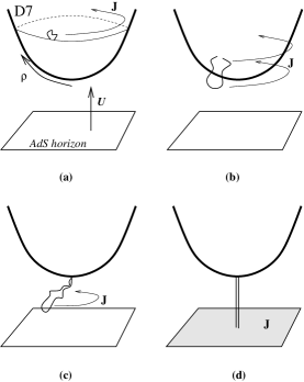
Figure 1: The proposed transition as the R-charge $J$ (the angular momentum in the horizontal plane) is taken large. The D7 brane, shown schematically, is warped by the geometry in the radial direction; gravity pulls down in the figure, along the coordinate $U=\sqrt{\rho^{2}+\rho_{\perp}^{2}}$, and the AdS horizon is shown as a horizontal plane. (a) A small string with moderate $J$ orbits around the end of the D7 brane. (b) As $J\to J_{*}$ the string distends and moves off the orbit shown in (a). (c) The ends of the string descend to the origin of the D7 brane, while its middle extends below the D7 brane and carries the angular momentum $J$. (d) At $J=J_{*}$ the string reaches the horizon, which absorbs the angular momentum, leaving two long stationary strings — unbound (s)quarks.

We therefore seek a null geodesic at a constant point in physical space $x^{1},x^{2},x^{3}$ and moving in time and around an equator of the $S^{3}$, e.g. the curve $\theta=0$. A particle moving on such a curve will have both large energy $E$ and large charge $J$. The effective Lagrangian for a particle describing this kind of motion is

$$\mathcal{L}=\alpha^{\prime}\left[-\frac{\rho^{2}+\rho_{\perp}^{2}}{\sqrt{\lambda}}\dot{t}^{2}+\frac{\sqrt{\lambda}}{\rho^{2}+\rho_{\perp}^{2}}(\dot{\rho}^{2}+\dot{\rho_{\perp}}^{2})+\frac{\sqrt{\lambda}\rho^{2}}{\rho^{2}+\rho_{\perp}^{2}}\dot{\psi}^{2}\right]\ ,$$

where the $\cdot$ means the derivative with respect to the affine parameter. The null condition $\mathcal{L}=0$ gives

$$\dot{\rho}^{2}+\dot{\rho}_{\perp}^{2}+\frac{J^{2}}{\lambda}\left(\rho+\frac{\rho_{\perp}^{2}}{\rho}\right)^{2}=E^{2}\ ,$$

where $E$ and $J$ are the conserved energy and angular momentum associated with the Killing vectors $\partial/\partial t$ and $\partial/\partial\psi$ respectively. This is the dynamics of a particle moving in a potential $V(\rho,\rho_{\perp})=\rho\ +\rho_{\perp}^{2}/\rho$. Note that the D7-brane is located at $\rho_{\perp}=m_{Q}$. If the string itself were fixed to be at $\rho_{\perp}=m_{Q}$, then the minimum of the potential would be at $\rho=\rho_{\perp}=m_{Q}$. However, the string (except for its ends) is free to move to any value of $\rho_{\perp}$, and with no constraint on $\rho_{\perp}$ the minimum of the potential lies at $\rho_{\perp}\to 0$. This shows that there is no stable geodesic with the properties that we are seeking. In particular, a particle, or an unconstrained piece of string, on the above trajectory wants to fall off the D7-brane toward the horizon of the AdS space.

This result shows the $Q\Phi^{J}\tilde{Q}$ states are fully unstable, not metastable, for $J\gg\sqrt{\lambda}$. In particular, we are led to a speculation concerning the nature of that instability. These states correspond to open strings with both ends on the D7-brane; while the ends cannot move off the D7-brane, the bulk of the string worldsheet may be expected, according to the above computation, to fall off the D7-brane toward the horizon. This is illustrated in Fig. 1. Once the string becomes an extended object, and no longer acts as a massless point particle as viewed in ten dimensions, it will no longer follow the orbit shown in Fig. 1a. (This represents the onset of the loss of efficient trapping in the gauge theory.) Instead, the string will move to a lower orbit, with more of the angular momentum being carried by the lower regions of the string where the energy cost is less due to the redshift of the metric. For large enough $J$, the ends of the string will move almost to the origin of the D7 brane, with the angular momentum mainly carried by the center of the string, which continues to orbit around the origin. As $J$ increases further, the string will become longer still, and eventually the string will hit the horizon, at which point the angular momentum will dissolve into the horizon, as shown in Fig. 1d. In this case the two (s)quarks, represented by two independent straight strings, are unbound, and the $J$ adjoints are free to move away from the (s)quarks and from each other.

For just slightly smaller $J$, corresponding to the limit of Fig. 1c just before it transitions to Fig. 1d, the binding of the generalized quarkonium state is very weak. In this regime a Born-Oppenheimer calculation will be valid, in which the ends of the string are held fixed, a Wilson-loop computation is performed first, and the motion of the ends of the string is quantized second. This then motivates us to carry out the Wilson-loop calculation, which should show the unbinding transition at $J=J_{*}$.

3 A Wilson Loop and the Unbinding of Adjoints

The Wilson-loop computation in field theory corresponds, as is well known, to the problem of computing the energy of an appropriate semiclassical string sitting within a supergravity background. We proceed in perfect analogy with the hydrogen molecule calculation of the effective potential between the two protons induced by the electrons. Instead of studying (s)quarks of finite mass $m$ at a distance of order $1/m$, we will take $m$ to infinity while fixing the distance $L$ between the heavy squark and antisquark. Meanwhile we keep $m_{\Phi}$ fixed. If we are in the regime where the $\Phi$ particles are trapped, and $L<m_{\Phi}^{-1}$, then the $\Phi$ particles should spread out over a region whose size is of order $L$. If they are not trapped, they should spread out over a region whose size is of order $m_{\Phi}^{-1}$. We will see a transition between these two behaviors below. The results of this calculation will give us the effective potential. This potential will remain valid for (s)quarks of finite mass $m$ if the binding energy $E_{0}$ of the ground state for finite-mass quarks in this potential is small compared to $m$. For $m_{\Phi}$ sufficiently small, the potential must be of Coulomb type (by conformal invariance). A necessary condition for small binding energy is that the coefficient of the Coulomb term — the effective $\alpha$ — be small compared to 1. This is always true sufficiently near the transition point $J=J_{*}$, and this will allow us to compute $J_{*}$. Note however that for any fixed $\lambda$ there need not exist any bound states well-described by the Born-Oppenheimer method, and indeed we will see that such states are not generic.

The easiest way to study this problem initially is to take $m_{\Phi}$ to zero. In this case we need only make appropriate modifications of the original computation of the Wilson loop by Maldacena [10] and by Rey and Yee [11] to determine the coefficient of the $1/L$ potential between infinitely heavy sources in the fundamental representation of $SU(N)$ in ${\cal N}=4$ supersymmetric Yang-Mills. It was found that the coefficient was $-4\pi^{2}\sqrt{\lambda}/[\Gamma(1/4)]^{4}$ when the sources are antiparticles of one another. Maldacena also considered the case when the sources couple differently to the scalar fields of the ${\cal N}=4$ theory, a possibility we will return to in just a moment.

To understand the calculation we wish to perform, we need to examine the theory carefully. The ${\cal N}=4$ theory has an $SO(6)$ R-symmetry, and a sextuplet of scalar fields which it is convenient to organize into three complex scalars $\Phi_{i}$. To preserve the maximal supersymmetry, a BPS-saturated source in the fundamental representation of $SU(N)$ must be a massive vector multiplet, which preserves an $SO(5)$ subgroup of this symmetry. Alternatively, we can preserve half the supersymmetry if we add a source which is a massive ${\cal N}=2$ hypermultiplet; this source preserves an $SO(4)$ subgroup of the R-symmetry. In both cases, the source-antisource state appropriate to a Wilson loop computation breaks supersymmetry (in general), but preserves the same $SO(5)$ [or $SO(4)$] subgroup as the isolated BPS source. In the computation of [10, 11], this source-antisource state is described as a string whose ends lie at the boundary of AdS a distance $L$ apart, and which are oriented on the $S^{5}$ so as to preserve the appropriate $SO(5)$ symmetry [or $SO(4)$.]

We may now ask that the bulk of the string worldsheet be allowed to rotate around an equator of the $S^{5}$, so that it picks up a charge $J$ with respect to an $SO(2)\approx U(1)$ subgroup of the $SO(5)$ [or $SO(4)$.] This corresponds to the source-antisource state binding to $J$ complex scalars $\Phi$ which are charged with respect to this $U(1)$. (Calculations of this sort of state have also been undertaken in various papers, especially in [13, 14, 9] where a very similar method was needed.) For the case relevant to the D3-D7 system we have been considering in this paper, we imagine we introduce an infinitely massive hypermultiplet $Q,\tilde{Q}$ which couples to the scalar field $\Phi_{3}$ (using a D7-brane at $x^{8}=m\to\infty,x^{9}=0$.) We may then add $J$ scalars $\Phi_{1}$ to the state built from a (s)quark and anti(s)quark by allowing the string to rotate in the $x^{4}$–$x^{5}$ plane.

Since the theory with $m_{\Phi}=0$ and $m=\infty$ is conformal ${\cal N}=4$ Yang-Mills, we know the potential will be of the form $V(L)=f(\lambda,J)/L$. Our simplest goal is to determine $f(\lambda,J)$. More generally we wish to determine the shape of the string corresponding to a given $\lambda$ and $J$. We will now present this calculation, which exhibits a trapping transition.

The computation is slightly more complicated than the prototype [10, 11], since a third coordinate comes into play. However, the mathematics largely reduces to one of Maldacena’s other computations, as we will see. A even more similar computation was performed by Tseytlin and Zarembo in [14], and our techniques follow theirs. On the surface it would appear that we are about to repeat their computation, but the details of their solutions are crucially different. In particular, we choose different boundary conditions from [14]. Our boundary condition corresponds (as we will see) to a distribution of the global $U(1)$ charge which is regular near the source and antisource; that of [14] is singular (though integrable.) The instability found at weak-coupling in [14] does not apply to our computation.

The equations for the shape of the string and its energy are mathematically equivalent to the computation of [10] in which the source and antisource are not each other’s antiparticles. Maldacena introduced two massive vector multiplets which preserved different $SO(5)$ symmetries, leaving an $SO(4)$. An angle $\Delta\chi$ enters this computation, describing how badly aligned are the $SO(5)$s preserved by the source and antisource; more intuitively, it specifies the angular separation on the $S^{5}$ of the two ends of the string as they approach the boundary. For $\Delta\chi=0$ the source and antisource are antiparticles, while for $\Delta\chi=\pi$ the state of the source and antisource is BPS-saturated and the binding energy is zero. In this case $V(L)=f(\lambda,\Delta\chi)/L$; Maldacena found an implicit form for the function $f$. We will see that this function reappears in the calculation below, but with a very different interpretation.

3.1 The Calculation

We will consider a rectangular Wilson loop of length $L$ and duration $T$, and we consider the limit $T\rightarrow\infty$ in order to extract the potential energy between sources at a distance $L$ from one another. This calculation is dual to a computation of the energy of a string whose ends lie on the boundary of AdS and are separated by a distance $L$ in the spatial coordinates of the gauge theory.

We can use the Polyakov action to describe the semiclassical string worldsheet

$$S=-\frac{1}{4\pi\alpha^{\prime}}\int d\tau d\sigma(-\gamma)^{1/2}\gamma^{\alpha\beta}G_{MN}\partial_{\alpha}X^{M}\partial_{\beta}X^{N}$$

with appropriate boundary conditions at the end points, which lie at $\rho_{\perp}=\infty$.

We are looking for a stationary configuration of the string such that $\chi=0$. The string should be rotating around an equator of $S^{3}$, parameterized by the angle $\psi$; we set $\psi=\omega t$ where $\omega$ is a constant. We put the (s)quark (one end of the string) at $X(\rho_{\perp}=\infty)=L/2$ and the anti(s)quark (the other end) at $X(\rho_{\perp}=\infty)=-L/2$, in order that string configuration be symmetric about $X=0$. We will find it useful to employ the coordinates $U$ and $\theta$,

$$U^{2}=\rho^{2}+\rho_{\perp}^{2}\quad,\quad\theta=\arctan\frac{\rho}{\rho_{\perp}}\ .$$

$U$ is the usual $AdS_{5}$ radial coordinate, and $\theta$ is a polar angle on the five-sphere. We are interested in solutions in which the source itself is not associated with any global charge, and so we expect that $\theta\to 0$ and $X(U)$ goes to the solution of [10, 11] as $U\to\infty$.

Using the conformal gauge $\gamma_{\alpha\beta}=\eta_{\alpha\beta}$ , the required portion of the string action (setting the string tension equal to 1) becomes

$$S=-\frac{T}{4\pi}\int d\sigma\mathcal{L}\equiv TS_{0}$$

$$\mathcal{L}=\frac{\rho^{2}+\rho_{\perp}^{2}}{\sqrt{\lambda}}(\dot{t}^{2}+X^{\prime 2})+\frac{\sqrt{\lambda}}{\rho^{2}+\rho_{\perp}^{2}}(\rho^{\prime 2}+\rho_{\perp}^{\prime 2}-\rho^{2}\dot{\psi}^{2})\ ,$$ (2)

where $\dot{}\equiv\partial_{\tau}$ and ${}^{\prime}\equiv\partial_{\sigma}$. Using the coordinates $U$ and $\theta$, we can separate $\mathcal{L}$ into two parts which depend only on the $AdS_{5}$ coordinates and the $S^{5}$ coordinates, respectively. Fixing $\tau=t$,

$$\mathcal{L}=\frac{U^{2}}{\sqrt{\lambda}}(1+X^{\prime 2})+\frac{\sqrt{\lambda}}{U^{2}}U^{\prime 2}+\sqrt{\lambda}(\theta^{\prime 2}-\omega^{2}\sin^{2}\theta)\ .$$ (3)

The equations of motion for the $AdS_{5}$ coordinates $U$, $X$ decouple from that of the $S^{5}$ coordinate $\theta$.

$$X^{\prime} = gU_{0}^{2}/U^{2}$$ (4)

$$\frac{U^{\prime 2}}{U^{2}}+\frac{g^{2}}{\lambda}\frac{U_{0}^{4}}{U^{2}}-\frac{1}{\lambda}U^{2} = \frac{g^{2}-1}{\lambda}U_{0}^{2}$$ (5)

$$\theta^{\prime 2}+\omega^{2}\sin^{2}\theta = \omega^{2}\sin^{2}\theta_{0}\ .$$ (6)

Here $g$ is a (dimensionless) constant of integration. At the midpoint of the string $X=0$, where $\theta^{\prime}=0$ and $U^{\prime}=0$, $\theta$ reaches its maximum value $\theta_{0}$ and $U$ reaches its minimum value $U_{0}$. The constraint equation resulting from the conformal freedom of the worldsheet metric in the Polyakov action,

$$\frac{U^{2}}{\sqrt{\lambda}}(-1+x^{\prime 2})+\frac{\sqrt{\lambda}}{U^{2}}U^{\prime 2}+\sqrt{\lambda}(\theta^{\prime 2}+\omega^{2}\sin^{2}\theta)=0\ ,$$

gives the relation

$$g^{2}=1-\Omega^{2}\sin^{2}\theta_{0}\quad,\quad\Omega\equiv\frac{\sqrt{\lambda}\omega}{U_{0}}\ .$$ (7)

The state we are studying has angular momentum $J$ and energy $E$,

$$J=\frac{\delta S_{0}}{\delta\omega}=\frac{\omega\sqrt{\lambda}}{2\pi}\int d\sigma\sin^{2}\theta$$ (8)

$$E=\omega\frac{\delta S_{0}}{\delta\omega}-S_{0}=\frac{1}{2\pi}\frac{1}{\sqrt{\lambda}}\int d\sigma U^{2}\ .$$ (9)

Note that the energy is divergent and must be regulated; we want the negative potential energy between the source and antisource, so we must carefully subtract the divergent masses of the sources, as in [10, 11].

Remarkably, part of the solution to these equations is of the same form as one of Maldacena’s computations. In particular, the configuration $X=X(U)$ is the same as that of a string stretched between two D3-branes located at the boundary with an angular separation on the $S^{5}$ if we identify $g^{2}$ in our equations with $1-l^{2}$ in equations (4.10)–(4.12) of [10]. The string configuration $X=X(U)$ is obtained from Eq. (5)

$$X=\frac{\sqrt{\lambda}g}{U_{0}}I(g,U/U_{0})\ ,$$ (10)

where

$$I(g,U/U_{0}) = \int_{1}^{U/U_{0}}dy\frac{1}{y^{2}\sqrt{(y^{2}-1)(y^{2}+g^{2})}}$$

$$= \frac{1}{g^{2}}\left[E\left(\sin^{-1}(U_{0}/U),ig\right)-F\left(\sin^{-1}(U_{0}/U),ig\right)\right]\ .$$

(Here $E$, $F$ and later $K$ are elliptic integrals, with conventions defined in Appendix C.) The string end point is located at $(X,U)=(L/2,\infty)$, which determines $U_{0}$ for a given $g$:

$$\frac{L}{2}=\frac{\sqrt{\lambda}g}{U_{0}}I(g)$$ (12)

where

$$I(g)\equiv I(g,U/U_{0}\rightarrow\infty)={1\over g^{2}}\left[E(ig)-K(ig)\right]\ .$$ (13)

The relation between $\theta(U)$ in our computation and the mathematically-related angular-separation variable in [10] is not so direct, however. The string configuration $\theta=\theta(U)$ is obtained from Eqs. (6) and (10):

$$\int_{0}^{\theta}\frac{d\theta}{\sqrt{1-\frac{\sin^{2}\theta}{\sin^{2}\theta_{0}}}}=\sqrt{1-g^{2}}\int_{U/U_{0}}^{\infty}\frac{dy}{\sqrt{(y^{2}-1)(y^{2}+g^{2})}}\ .$$ (14)

Here we used $\theta(U\rightarrow\infty)\rightarrow 0$, consistent with the boundary condition. While the right-hand side of this equation appears verbatim in equation (4.10) of [10], the left-hand side is significantly different in all respects.

Equation (14) may also be written as

$$\sin\theta_{0}\ F\Big{(}\sin^{-1}(\sin\theta/\sin\theta_{0}),\sin\theta_{0}\Big{)}=\sqrt{1-g^{2}}\ F\Big{(}\sin^{-1}(U_{0}/U),ig\Big{)}\ .$$

The condition that $\theta=\theta_{0}$ at $U=U_{0}$ gives the relation which determines $g$ for a given $\theta_{0}$:

$$\sin\theta_{0}\ K(\sin\theta_{0})=\sqrt{1-g^{2}}K(ig)\ .$$ (15)

Using the equations of motion, the angular momentum $J$ can be written as

$$J = \frac{\sqrt{\lambda}}{\pi}\int_{0}^{\theta_{0}}d\theta\frac{\sin^{2}\theta}{\sqrt{\sin^{2}\theta_{0}-\sin^{2}\theta}}$$ (16)

$$= \frac{\sqrt{\lambda}}{\pi}\Big{[}K(\sin\theta_{0})-E(\sin\theta_{0})\Big{]}\ .$$

The energy in Eq. (9) should be regularized by subtracting the masses of $Q$ and $\tilde{Q}$ because it includes infinite $Q$ and $\tilde{Q}$ masses.

$$EL = \frac{U_{0}}{\pi}\left[\int_{1}^{\infty}dy\left(\frac{y^{2}}{\sqrt{(y^{2}-1)(y^{2}+g^{2})}}-1\right)-1\right]$$ (17)

$$= -\frac{2\sqrt{\lambda}g^{3}}{\pi}[I(g)]^{2}$$

which again matches equation (4.13) of [10], but with quite a different interpretation, as we will now see.

Our solution is now complete: we can make one-to-one correspondence between the parameters in our equations with the physical quantities, $J$ and $E$. For a given $J$, there is a corresponding $\theta_{0}$ from the relation Eq. (16) and $g$ is determined from Eq. (15). Accordingly, $E$ is obtained from Eq. (17). Finally, $U_{0}$ is determined from the relation Eq. (12), and $U(X)$ can be implicitly found from Eq. (10).

However, it can be seen that the range of $J$ is restricted, and cannot be arbitrarily large. This is the sign of the instability which we have been seeking. The left side of Eq. (15) is an increasing function of $\theta_{0}$, while the right side is a decreasing function of $g$. The right-hand side of Eq. (15) has an upper-bound of $\pi/2$, which occurs when $g\rightarrow 0$, while the left-hand side diverges logarithmically as $\theta_{0}\rightarrow\pi/2$. Therefore, there exists an upper bound for $\theta_{0}$, which we will call $\theta_{*}$, with

$$\sin\theta_{*}\ K(\sin\theta_{*})=\frac{\pi}{2}$$ (18)

and correspondingly one for $J$, which we will call $J_{*}$:

$$J_{*}=\frac{\sqrt{\lambda}}{\pi}\Big{[}K(\sin\theta_{*})-E(\sin\theta_{*})\Big{]}\ .$$

Numerically, $\sin\theta_{*}\approx 0.793$ and $J_{*}\approx 0.22\sqrt{\lambda}$ .

To know what does happen when $J\rightarrow J_{*}$, we need to analyze the behavior of the string as $g\rightarrow 0$. Since $I(g)\rightarrow\pi/4$ as $g\rightarrow 0$ ($J\rightarrow J_{*}$),

$$\quad U_{0}\sim g\rightarrow 0\quad,\quad EL\sim-g^{3}\rightarrow 0\ .$$ (19)

This shows that $U_{0}$ touches the horizon and the interaction energy vanishes as $J\rightarrow J_{*}$. That is, for fixed $L$, the massless $\Phi$ particles completely unbind from the infinitely heavy (s)quark and anti(s)quark for $J>J_{*}$. As we will discuss further below, this implies that generalized quarkonium states also become unbound (for massless adjoints) for $J$ greater than $J_{*}$.

Figure 2: String configurations for $g=1$(dotted), $0.1$(thin solid), and $0$(thick solid) (equivalently, $J/J_{*}=0$, $0.9867$, and $1$, respectively) in the $X$-$U$ plane. Note the minimum value of $U$ is a decreasing function of $J$.

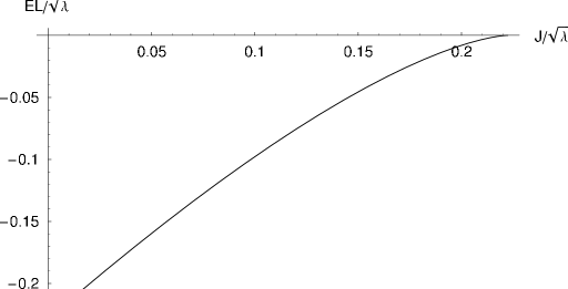
Figure 3: $E$ versus $J$

The relation between $E$ and $J$ (for fixed $L$) is plotted numerically in Figure 3 and is obtained in two limits ($J\rightarrow 0$ and $J\rightarrow J_{*}$) in Appendix A; the result is

$$EL \approx -\frac{4\pi^{2}\sqrt{\lambda}}{\left[\Gamma\left(\frac{1}{4}\right)\right]^{4}}\left(1-2\pi\frac{J}{\sqrt{\lambda}}+\dots\right)\quad,\quad J\rightarrow 0$$ (20)

$$EL \approx -\pi\left(\frac{2}{3}\right)^{3/2}\sqrt{\lambda}\left[\left(\frac{J_{*}-J}{\sqrt{\lambda}\sin\theta_{*}}\right)^{3/2}+\dots\right]\quad,\quad J\rightarrow J_{*}\ .$$ (21)

Note $|E|$ decreases as $J$ increases, as expected; the presence of the scalars in the state makes the binding energy smaller in magnitude. Interestingly, the relation between $E$ and $J$ is nonanalytic as $J\to J_{*}$, indicating a sharp transition.

It is interesting to ask where the scalar fields actually lie in the space between the source and antisource. We do not know the precise answer to this question, but some significant insight is obtained by examining the density of $J$ as a function of $x=X/[L/2]$, or as a function of $y=U/U_{0}$. For a given $g$, the density of $J$ is given by

$$\rho(y)\propto\frac{\sin^{2}\theta(y)}{\sqrt{(y^{2}-1)(y^{2}+g^{2})}}\quad,\quad\rho(x)\propto y^{2}\sin^{2}\theta(y)\ ,$$ (22)

where $\theta(y)$ is given in Eq. (14). This is illustrated in Figure 4. As can be seen, as $J\to J_{*}$ the scalars cluster at $U\sim U_{0}\to 0$; using the usual inverse relationship between the $U$ coordinate and the size of distributions in the field theory [1, 15], this strongly suggests that the scalars spread out, and thus the size of the state is diverging, as $J\to J_{*}$.

$\begin{array}[]{c @{\hspace{0.25in}} c}\epsfbox{Jydensity.eps}\hfil\hskip 18.06749pt&\epsfbox[93-3428198]{Jxdensity.eps}\\[0.0pt] \mbox{(a)}\hfil\hskip 18.06749pt&\mbox{(b)}\\[0.0pt] \end{array}$

Figure 4: (a) Density of $J$ versus $y=U/U_{0}$ and (b) Density of $J$ versus $x=X/(L/2)$ in Eq. (22) for $g=0.1$ ($J/J_{*}\approx 0.9867$.)

In summary, we have found that in the case of infinitely massive (s)quarks and massless $\Phi$ adjoints, trapping occurs for $J<J_{*}\approx 0.22\sqrt{\lambda}$, decreasing in its effects as $J\to J_{*}$. For $J>J_{*}$, the adjoints do not bind to the sources, and the effective potential vanishes.

We have also considered how this calculation is modified if, as in [10], the string’s endpoints are at two different positions on the five-sphere. Without loss of generality we may take these positions to lie on the same great circle, one of them at $+\Delta\chi/2$ and one at $-\Delta\chi/2$. This computation, presented in Appendix B, shows qualitatively similar behavior; as $\Delta\chi$ increases, the value of $J$ at which the binding energy drops to zero decreases, until at $\Delta\chi=\pi$, where the state is BPS saturated, the binding energy is zero even for $J=0$. The curve in the $(J,\Delta\chi)$ plane where the binding energy vanishes is shown in Figure 6. Interestingly, the $U(X)$ curve and the binding energy are functions of only one combination of $J$ and $\Delta\chi$, given by the parameter $g$; in particular, for every $J<J_{*}$ with $\Delta\chi=0$, there exists a value of $\Delta\chi$ with $J=0$ that leads to the same curve $U(X)$ and the same binding energy. We do not know of a deep reason for this.

3.2 Discussion

Let us now consider what the Wilson loop computation implies for the generalized quarkonium states, for which $m_{\Phi}$ is not necessarily zero and $m\equiv m_{Q}$ is finite but much larger than $m_{\Phi}$. It is useful to break the discussion up using a couple of intermediate steps.

For infinite $m$ but nonzero $m_{\Phi}$, we expect the new mass-scale to introduce some new physics at a radial position $U\propto m_{\Phi}$ in the AdS space. Since the theory is no longer conformal, the potential will now be $V(L)=f(\lambda,J;m_{\Phi}L)/L$. For instance, if all six scalars receive positive masses, as in the ${\cal N}=1^{*}$ theory [16], then we expect the AdS space is effectively cut off at $U_{min}\sim m_{\Phi}$. This means that our solutions will be valid only until $U_{0}$ reaches $m_{\Phi}$. This in turn means that the shape of the string, and the corresponding effective potential, will change once $L>m_{\Phi}^{-1}$. Indeed, the calculation should eventually match on to that of [9]. For large $L$, the string will lie at $U=U_{min}$ for most of the region $-L/2\ <\ X\ <\ L/2$, and we expect the $\theta$-coordinate of the string to relax to $\pi/2$, as this should minimize the energy of the configuration. This gives [9]

$$E\approx\sqrt{{\mathcal{T}}^{2}L^{2}+m_{\Phi}^{2}J^{2}}\qquad(U_{min}\sim m_{\Phi})\ .$$ (23)

Here ${\mathcal{T}}\sim\frac{\sqrt{\lambda}}{2\pi}m_{\Phi}^{2}$ is the tension of a standard flux tube in the gauge theory. Thus, the potential becomes linear in $L$ for sufficiently large $L$ and fixed $J$, and becomes linear in $J$ for fixed $L$ and sufficiently large $J\gg\sqrt{\lambda}$. The regions with different behaviors are shown in Figure 5. Note all the transitions are cross-overs; there are no phase transitions once $m_{\Phi}$ is nonzero.

Figure 5: The various regimes for nonzero $m_{\Phi}$. The diagonal dashed line is $J=\frac{\sqrt{\lambda}}{2\pi}m_{\Phi}L$. The potential goes as $1/L$ in the lower-left region, as $Jm_{\Phi}$ in the upper left region, and as $L$ times the flux-tube tension (of order $\sqrt{\lambda}m_{\Phi}^{2}$) in the lower-right region. All borders between regions are cross-overs; there are no sharp transitions.

For finite $m_{Q}$ and $m_{\Phi}=0$, on the other hand, the static Wilson loop we have been studying is no longer physical; instead the (s)quark and anti(s)quark must be put in orbit around each other. We have not attempted to examine this more complex dynamical problem carefully for general $J$, but in the regime $J\approx J_{*}$ the situation is under control. As we have discussed earlier, in this regime the force between the (s)quark and anti(s)quark is small and their motion is slow and nonrelativistic, justifying a Born-Oppenheimer approach. The effective potential for the slow (s)quark and anti(s)quark is given by the Wilson loop calculation we just performed. As long as $\alpha_{{\rm eff}}\equiv EL$, as given in Eq. (21), is small compared to 1 (as becomes true in the regime $J\approx J_{*}$), then we would expect that the heavy particles will move with a velocity $v\sim\alpha_{{\rm eff}}\ll 1$, as required.

However, to see whether and when this computation is valid, we must self-consistently solve for $L$, given a fixed quark mass $m_{Q}$. The scaling of the various quantities as $g\to 0$ is now different from the scaling relation (19), which was obtained holding $L$ fixed. Since $L=(\alpha_{{\rm eff}}m_{Q})^{-1}$ in a Coulomb system and $U_{0}\sim\sqrt{\lambda}g/L$, the scaling of the various quantities with $g\sim(J_{*}-J)^{1/2}\lambda^{-1/4}$ as $g\to 0$ is

$$\alpha_{{\rm eff}}=EL\sim\lambda^{1/2}g^{3},\quad L\sim\lambda^{-1/2}g^{-3},\quad E\sim\lambda g^{6},\quad U_{0}\sim\lambda g^{4}\ .$$

If we only required $\alpha_{{\rm eff}}\ll 1$, we would allow $J_{*}-J\ll\lambda^{1/4}$. But this is not sufficient. We must also require $U_{0}\ll m_{Q}$, so that our Wilson line computation with strings that extend to infinity bears some relation to the calculation with strings that extend only to the D7 brane at $U=m_{Q}$. Furthermore, we must also require $L\gg\sqrt{\lambda}/m_{Q}$, the trapping scale, which we showed in [4] also sets the scale of the (s)quark and anti(s)quark wave functions for the trapped states. The last condition requires $\alpha_{{\rm eff}}\ll 1/\sqrt{\lambda}\ll 1$. This in turn requires $J_{*}-J\sim\lambda^{-1/6}\ll 1$! This means that for most values of $\lambda$ there is no integer $J$ for which there is a state described by a Born-Oppenheimer calculation.

Still, this scaling is still sufficient for our purposes: for fixed $J$, there is always some range of $\lambda$ for which the calculation is valid. If we follow any particular state of definite $J$ as $\lambda$ is decreased adiabatically, the state becomes unbound at $J=J_{*}$ by passing, rather swiftly, through a regime in which it is described by our Born-Oppenheimer calculation, grows much larger than its typical size $\sqrt{\lambda}/m_{Q}$, and unbinds when $J_{*}\sim\sqrt{\lambda}$ reaches $J$. Consequently, for any fixed $\lambda$, there are no bound states with $J>J_{*}$. All states with low spin, no radial excitation, and $J_{*}-J>\lambda^{-1/6}$ have adjoints trapped in a small region. This is consistent with our earlier conjectures; what we have learned with these calculations is how rapidly the transition occurs.

Finally, let us consider what will happen if both $m_{\Phi}$ and $m_{Q}$ are nonzero, with $m_{\Phi}\ll m_{Q}$. In this case we expect a cross-over, as in the Wilson-loop computation, to occur in the regime $J\approx J_{*}$. As before, the Born-Oppenheimer regime exists at $J_{*}-J\sim\lambda^{-1/6}$. The calculation of the Coulombic potential and its coefficient need only be modified by confinement effects at an even smaller value of $J_{*}-J$, at the point where the untrapping of the adjoints allows them to reach the confinement scale $\Lambda\sim 1/m_{\Phi}$. Again there is a cross-over, a rather sharp one, in which, for fixed $J$ and decreasing $\lambda$, each bound state goes from a object of size $\sim 1/m_{Q}$ with trapped adjoints to a larger confined state of a size $\sim 1/m_{\Phi}$. Equivalently, at any fixed $\lambda$, there is a sharp transition in the spectrum where low-spin zero-radial-excitation states with $J<J_{*}$ have the adjoints trapped in a region of size $\sim 1/m_{Q}$, while states with $J>J_{*}$ spread their adjoints over a region of size of order $1/m_{\Phi}$, with the (s)quark wave functions somewhat more compact.

Of course, all of these results are modified at finite $N$. We expect the potential energy does not change dramatically. A more important effect is that the strings of moderate $J$ ($1\ll J\ll\sqrt{\lambda}$) and $L\ll 1/m_{\Phi}$ can decay, by emission of closed strings carrying nonzero charge $J^{\prime}$, to open strings with charge $J-J^{\prime}$. In other words, generalized quarkonium states can decay, via emission of states of the ${\cal N}=4$ or ${\cal N}=1^{*}$ theory carrying the global $U(1)$ charge. The typical closed string carrying charge $J^{\prime}$ will correspond (in a confining theory — recall that the confinement scale $\Lambda\sim m_{\Phi}$ for large $\lambda$) to a hadron with mass of order $J^{\prime}m_{\Phi}$. Meanwhile, for a string with endpoints separated by a length $L$, $\partial E/\partial J\sim 1/L\gg m_{\Phi}$, implying that these decays are kinematically allowed. The same is true for dynamical generalized quarkonium, for which $L\sim\sqrt{\lambda}m_{Q}^{-1}$ when $J$ is not near $J_{*}$. The phase space for these decays is substantial, but by dialing the coupling $1/N$ the widths of the generalized quarkonium states can be made arbitrarily small compared to their masses. We would therefore expect them to remain as sharp resonances for large but finite $N$.

Finally, let us address the issue of how the physics of large $\lambda$ matches on to that at small $\lambda$. Since trapping occurs for $J<J_{*}\sim\sqrt{\lambda}$, it simply need not occur for theories with $\lambda<1$. This agrees with our understanding of these generalized quarkonium states in perturbation theory, which suggests that their size should be of order $m_{\Phi}^{-1}$ and that they should become unbound as $m_{\Phi}\to 0$. However, it is worth considering the possibility that the $J=1$ state in a QCD-like theory with additional adjoint matter might, in very favorable circumstances, exhibit adjoint trapping. The quark masses $m_{Q}$ would need to lie not far above $\Lambda$ (so that $\lambda(m_{Q})\sim 1$) with the adjoint masses lighter than $\Lambda$, and perhaps additional binding interactions (such as a Yukawa interaction between the quarks) might also be needed. This possibility could be explored numerically, though rather large $N$ might be required in order to stabilize the state against decay. Although a long-shot, the observation of adjoint trapping in lattice gauge theory simulations would certainly be remarkable.

Appendix A The behavior near $J=J_{*}$

To get the behavior of $J$ near $J_{*}$ as $g\rightarrow 0$, we expand each side of Eq. (15) with respect to $\epsilon\equiv\sin\theta_{*}-\sin\theta_{0}$ and $g^{2}$ respectively

$$(\sin\theta_{*}-\epsilon)K(\sin\theta_{*}-\epsilon)=\sqrt{1-g^{2}}\int_{1}^{\infty}\frac{dy}{\sqrt{(y^{2}-1)(y^{2}+g^{2})}}$$ (24)

where $\sin\theta_{*}$ is determined by Eq. (18). After expanding,

$$\epsilon=\frac{3\pi/8}{K(\sin\theta_{*})+\sin\theta_{*}K^{\prime}(\sin\theta_{*})}g^{2}+O(g^{4})\ .$$ (25)

Expansion of $J$ near $J_{*}$ gives

$$J_{*}-J=\epsilon\frac{\sqrt{\lambda}}{\pi}[K^{\prime}(\sin\theta_{*})-E^{\prime}(\sin\theta_{*})]+O(\epsilon^{2})\ .$$ (26)

Therefore, as $J\rightarrow J_{*}$ ($g\rightarrow 0$),

$$\sin\theta_{*}-\sin\theta_{0} \approx \frac{3\pi/8}{E(\sin\theta_{*})/\cos^{2}\theta_{*}}g^{2}$$

$$J_{*}-J \approx \frac{\sqrt{\lambda}}{\pi}\frac{\sin\theta_{*}E(\sin\theta_{*})}{\cos^{2}\theta_{*}}(\sin\theta_{*}-\sin\theta_{0})$$

$$EL \approx -\frac{\pi\sqrt{\lambda}}{8}g^{3}\approx-\pi\left(\frac{2}{3}\right)^{3/2}\sqrt{\lambda}\left(\frac{J_{*}-J}{\sin\theta_{*}\sqrt{\lambda}}\right)^{3/2}\ .$$ (27)

It is straightforward to get the behavior as $J\rightarrow 0$ ($g\rightarrow 1$),

$$\sin\theta_{0} = \frac{[\Gamma(1/4)]^{2}}{2\pi^{3/2}}(1-g)^{1/2}+O[(1-g)^{3/2}]$$

$$J = \frac{\sqrt{\lambda}}{4}\sin^{2}\theta_{0}+O(\sin^{4}\theta_{0})$$

$$EL \approx E_{0}L+\zeta J\ .$$ (28)

where $E_{0}L=-4\pi^{2}\sqrt{\lambda}/[\Gamma(1/4)]^{4}$ and $\zeta=8\pi^{3}/[\Gamma(1/4)]^{4}$ .

From the expansion of $I(g,y)$ for small $g$,

$$I(g,y) \!\!\!=\!\!\! \frac{1}{2}\left(\frac{\sqrt{y^{2}-1}}{y}+\sec^{-1}(y)\right)-\frac{g^{2}}{16}\left(\frac{(3y^{2}+2)\sqrt{y^{2}-1}}{y^{4}}+3\sec^{-1}(y)\right)+O(g^{4})$$ (32)

$$\rightarrow \left\{\begin{array}[]{ll}\left(1-\frac{g^{2}}{2}\right)\sqrt{2(y-1)}+O[g^{4},(y-1)^{3/2}]\quad,\quad y\rightarrow 1\\ \\ \frac{\pi}{4}-\frac{1}{3y^{3}}-\frac{3\pi g^{2}}{32}+O(g^{4},1/y^{5})\quad,\quad y\rightarrow\infty\end{array}\right.$$

where $y=U/U_{0}$, we can get the shape of the string near $U=U_{0}$ or near the boundary ($U/U_{0}\rightarrow\infty$) as $J\rightarrow J_{*}$,

$$x^{2} = \frac{32}{\pi^{2}}\left(1-\frac{g^{2}}{4}\right)(y-1)+O[g^{4},(y-1)^{3/2}]\quad,\quad y\rightarrow 1$$ (33)

$$1-x = \frac{4}{3\pi}\left(1+\frac{3g^{2}}{8}\right)\frac{1}{y^{3}}+O(g^{4},1/y^{5})\quad,\quad y\rightarrow\infty$$ (34)

where $x=X/(L/2)$.

Appendix B String Stretched Between Two D7-Branes at Different Angles

We consider a stationary string configuration rotating on $S^{3}$ and with its ends on two parallel D7-branes, located at $U=\infty$ with angular separation $\Delta\chi$ (here $\chi$ is the polar coordinate in the $x^{8}-x^{9}$ plane, as in the metric (1).)

After using conformal gauge and fixing $\tau=t$

$$\mathcal{L}=\frac{U^{2}}{\sqrt{\lambda}}(1+x^{\prime 2})+\frac{\sqrt{\lambda}}{U^{2}}U^{\prime 2}+\sqrt{\lambda}(\theta^{\prime 2}+\cos^{2}\theta\ \chi^{\prime 2}-\omega^{2}\sin^{2}\theta)\ ,$$ (35)

where ${}^{\prime}\equiv\partial_{\sigma}$. Again the equations of motion for $U,X$, which are the same as for $\Delta\chi=0$, decouple from the equations of motion for $\theta,\chi$:

$$X^{\prime} = gU_{0}^{2}/U^{2}$$ (36)

$$\frac{U^{\prime 2}}{U^{2}}+\frac{g^{2}}{\lambda}\frac{U_{0}^{4}}{U^{2}}-\frac{1}{\lambda}U^{2} = \frac{g^{2}-1}{\lambda}U_{0}^{2}$$ (37)

$$\chi^{\prime} = l\frac{U_{0}\cos\theta_{0}}{\sqrt{\lambda}}\frac{1}{\cos^{2}\theta}$$ (38)

$$\theta^{\prime 2}+\omega^{2}\sin^{2}\theta+l^{2}\frac{U_{0}^{2}\cos^{2}\theta_{0}}{\lambda}\frac{1}{\cos^{2}\theta} = \omega^{2}\sin^{2}\theta_{0}+l^{2}\frac{U_{0}^{2}}{\lambda}\ ,$$ (39)

where $g$ and $l$ are (dimensionless) constants of integration. $\theta_{0}$ and $U_{0}$ are the values of $\theta$ and $U$ at the midpoint of the string, $X=0$, where we take $\chi=0$. At the endpoints of the string $X\to\pm L/2$, $\theta\to 0$, $U\to\infty$, and $\chi\to\pm\Delta\chi/2$.

The constraint equation resulting from the conformal freedom of the worldsheet metric in the Polyakov action is

$$\frac{U^{2}}{\sqrt{\lambda}}(-1+x^{\prime 2})+\frac{\sqrt{\lambda}}{U^{2}}U^{\prime 2}+\sqrt{\lambda}(\theta^{\prime 2}+\cos^{2}\theta\chi^{\prime 2}+\omega^{2}\sin^{2}\theta)=0\ .$$

This gives the relation

$$g^{2}+l^{2}=1-\Omega^{2}\sin^{2}\theta_{0}\quad,\quad\Omega\equiv\frac{\sqrt{\lambda}\omega}{U_{0}}\ .$$ (40)

As before, the state has angular momentum $J$ and (divergent) energy $E$,

$$J=\frac{\delta S_{0}}{\delta\omega}=\frac{\omega\sqrt{\lambda}}{2\pi}\int d\sigma\sin^{2}\theta$$ (41)

$$E=\omega\frac{\delta S_{0}}{\delta\omega}-S_{0}=\frac{1}{2\pi}\frac{1}{\sqrt{\lambda}}\int d\sigma U^{2}\ .$$ (42)

The string configuration is described by the equations :

$$\int_{0}^{\theta}d\theta\frac{\cos\theta}{\sqrt{(1-\frac{\sin^{2}\theta}{\sin^{2}\theta_{0}})(\cos^{2}\theta+\frac{l^{2}}{\Omega^{2}})}}=\sqrt{1-l^{2}-g^{2}}\int_{U/U_{0}}^{\infty}\frac{dy}{\sqrt{(y^{2}-1)(y^{2}+g^{2})}}$$ (43)

which can be written as

$$\frac{\Omega}{\sqrt{\Omega^{2}+l^{2}}}\sin\theta_{0}\ F\left(\sin^{-1}\left[\frac{\sin\theta}{\sin\theta_{0}}\right],\frac{\Omega\sin\theta_{0}}{\sqrt{\Omega^{2}+l^{2}}}\right)=\sqrt{1-g^{2}-l^{2}}\ F\Big{(}\sin^{-1}(U_{0}/U),ig\Big{)}\ ,$$

$$\frac{\Delta\chi}{2}-\chi = \frac{l\cos\theta_{0}}{\Omega\sin\theta_{0}}\int_{0}^{\theta}d\theta\frac{1}{\cos\theta\sqrt{(1-\frac{\sin^{2}\theta}{\sin^{2}\theta_{0}})(\cos^{2}\theta+\frac{l^{2}}{\Omega^{2}})}}$$

$$= \frac{l\cos\theta_{0}}{\sqrt{\Omega^{2}+l^{2}}}\Pi\left(\sin^{-1}\left[\frac{\sin\theta}{\sin\theta_{0}}\right],\sin^{2}\theta_{0},\frac{\Omega\sin\theta_{0}}{\sqrt{\Omega^{2}+l^{2}}}\right)\ ,$$

$$X=\frac{g\sqrt{\lambda}}{U_{0}}I(g,U/U_{0})$$ (45)

where $I(g,U/U_{0})$ is defined in Eq. (3.1).

The angular momentum and the regularized energy are given by

$$J = \frac{\sqrt{\lambda}}{\pi}\int_{0}^{\theta_{0}}d\theta\frac{\sin^{2}\theta\cos\theta}{\sqrt{(\sin^{2}\theta_{0}-\sin^{2}\theta)(\cos^{2}\theta+\frac{l^{2}}{\Omega^{2}})}}$$

$$= \frac{\sqrt{\lambda}}{\pi}\frac{\Omega^{2}}{\sqrt{\Omega^{2}+l^{2}}}\left[K\left(\frac{\Omega\sin\theta_{0}}{\sqrt{\Omega^{2}+l^{2}}}\right)-E\left(\frac{\Omega\sin\theta_{0}}{\sqrt{\Omega^{2}+l^{2}}}\right)\right]\ ,$$

$$EL=-\frac{2\sqrt{\lambda}g^{3}}{\pi}[I(g)]^{2}\ .$$ (47)

Parameters are determined by the equations matching the boundary conditions :

$$\int_{0}^{\theta_{0}}d\theta\frac{\cos\theta}{\sqrt{(1-\frac{\sin^{2}\theta}{\sin^{2}\theta_{0}})(\cos^{2}\theta+\frac{l^{2}}{\Omega^{2}})}}=\sqrt{1-l^{2}-g^{2}}\int_{1}^{\infty}\frac{dy}{\sqrt{(y^{2}-1)(y^{2}+g^{2})}}$$ (48)

which can be written as

$$\frac{\Omega\sin\theta_{0}}{\sqrt{\Omega^{2}+l^{2}}}\ K\left(\frac{\Omega\sin\theta_{0}}{\sqrt{\Omega^{2}+l^{2}}}\right)=\sqrt{1-g^{2}-l^{2}}\ K(ig)\ ,$$

$$\frac{\Delta\chi}{2} = \frac{l}{\Omega\sin\theta_{0}}\int_{0}^{\theta_{0}}d\theta\frac{1}{\cos\theta\sqrt{(1-\frac{\sin^{2}\theta}{\sin^{2}\theta_{0}})(\cos^{2}\theta+\frac{l^{2}}{\Omega^{2}})}}$$

$$= \frac{l\cos\theta_{0}}{\sqrt{\Omega^{2}+l^{2}}}\ \Pi\left(\sin^{2}\theta_{0},\frac{\Omega\sin\theta_{0}}{\sqrt{\Omega^{2}+l^{2}}}\right)\ ,$$

$$\frac{L}{2}=\frac{g\sqrt{\lambda}}{U_{0}}I(g)\ .$$ (50)

For given $J$ and $\Delta\chi$, $\theta_{0}$ and $\frac{l}{\Omega}$ are determined from Eq (B) and (B). For these values, $\Omega$, $l$, and $g$ are determined from Eq (48) and (40). For this value of $g$, $U_{0}$ is determined from Eq (50). Finally, $\omega$ is determined from the relation $\Omega=\frac{\sqrt{\lambda}\omega}{U_{0}}$.

The right hand side of Eq. (48) is bounded from above and the left-hand side can be written as $\frac{\sqrt{\lambda}}{\pi}J/\sin\theta_{0}+\frac{\sqrt{\lambda}}{\pi}\int_{0}^{\theta_{0}}d\theta\cos\theta\sqrt{1-\sin^{2}\theta/\sin^{2}\theta_{0}}/\sqrt{\cos^{2}\theta+l^{2}/\Omega^{2}}$ , where the integral in the second term is finite. Therefore the value of $J$ is finite for any value of $g$ and $l$. Since the string configuration in the $X$–$U$ plane and the corresponding energy have the same expressions as in the $\Delta\chi=0$ case, $J$ is finite when $U_{0}$ touches the horizon and the interaction energy vanishes as $g\rightarrow 0$. In particular, at $g=0$ the maximum value $\theta_{*}$ of $\theta_{0}$ satisfies

$$\frac{\sin\theta_{*}}{\sqrt{1+l^{2}\sin^{2}\theta_{*}}}\ K\left(\frac{\sqrt{1-l^{2}}\ \sin\theta_{*}}{\sqrt{1+l^{2}\sin^{2}\theta_{*}}}\right)=\ \frac{\pi}{2}\ ,$$

where we used $\Omega^{2}\sin^{2}\theta_{*}=1-l^{2}$ for $g=0$. This occurs for finite $J_{*}$, for any $l$, with $J_{*}$ reaching zero when $l=1$ and $\Delta\chi=\pi$. By numerical computation, we find the curve in the ($J$, $\Delta\chi$) plane where $E=0$; this curve is shown in Figure 6.

Figure 6: Curve in the ($J$, $\Delta\chi$) plane where $E=0$ ($g=0$).

Appendix C Elliptic Integrals

We use the following definitions of the elliptic integrals.

$$F(\varphi,k) = \int_{0}^{\varphi}\frac{d\theta}{\sqrt{1-k^{2}\sin^{2}\theta}}$$

$$E(\varphi,k) = \int_{0}^{\varphi}d\theta\sqrt{1-k^{2}\sin^{2}\theta}$$

$$\Pi(\varphi,n,k) = \int_{0}^{\varphi}\frac{d\theta}{(1-n\sin^{2}\theta)\sqrt{1-k^{2}\sin^{2}\theta}}$$

$$K(k) = F\left(\frac{\pi}{2},k\right)$$

$$E(k) = E\left(\frac{\pi}{2},k\right)$$

$$\Pi(n,k) = \Pi\left(\frac{\pi}{2},n,k\right)$$

In some references and math-computing programs, $F(\varphi,k^{2})$, $E(\varphi,k^{2})$, $\Pi(\varphi,n,k^{2})$, $K(k^{2})$, $E(k^{2})$ and $\Pi(n,k^{2})$ represent the same integral definitions.

References

- [1] J. M. Maldacena, “The large N limit of superconformal field theories and supergravity,” Adv. Theor. Math. Phys. 2, 231 (1998) [Int. J. Theor. Phys. 38, 1113 (1999)] [arXiv:hep-th/9711200]; for a review, see O. Aharony, S. S. Gubser, J. M. Maldacena, H. Ooguri and Y. Oz, “Large N field theories, string theory and gravity,” Phys. Rept. 323, 183 (2000) [arXiv:hep-th/9905111].
- [2] O. Aharony, A. Fayyazuddin and J. M. Maldacena, “The large N limit of field theories from three-branes in F-theory,” JHEP 9807, 013 (1998) [arXiv:hep-th/9806159]; A. Fayyazuddin and M. Spalinski, “Large N superconformal gauge theories and supergravity orientifolds,” Nucl. Phys. B 535, 219 (1998) [arXiv:hep-th/9805096].
- [3] A. Karch and E. Katz, “Adding flavor to AdS/CFT,” JHEP 0206, 043 (2002) [arXiv:hep-th/0205236].
- [4] S. Hong, S. Yoon and M. J. Strassler, “Quarkonium from the fifth dimension,” JHEP 0404, 046 (2004) [arXiv:hep-th/0312071].
- [5] A. Karch, E. Katz and N. Weiner, “Hadron masses and screening from AdS Wilson loops,” Phys. Rev. Lett. 90 (2003) 091601 [arXiv:hep-th/0211107].
- [6] V. N. Gribov, “Orsay lectures on confinement. (I, II and III)” arXiv:hep-ph/9403218, arXiv:hep-ph/9404332, arXiv:hep-ph/9905285.
- [7] M. Kruczenski, D. Mateos, R. C. Myers and D. J. Winters, “Meson spectroscopy in AdS/CFT with flavour,” JHEP 0307, 049 (2003) [arXiv:hep-th/0304032].
- [8] D. Berenstein, J. M. Maldacena and H. Nastase, “Strings in flat space and pp waves from super Yang Mills,” JHEP 0204, 013 (2002) [arXiv:hep-th/0202021].
- [9] E. G. Gimon, L. A. Pando Zayas, J. Sonnenschein and M. J. Strassler, “A soluble string theory of hadrons,” JHEP 0305, 039 (2003) [arXiv:hep-th/0212061].
- [10] J. M. Maldacena, “Wilson loops in large N field theories,” Phys. Rev. Lett. 80, 4859 (1998) [arXiv:hep-th/9803002];
- [11] S. J. Rey and J. T. Yee, “Macroscopic strings as heavy quarks in large N gauge theory and anti-de Sitter supergravity,” Eur. Phys. J. C 22, 379 (2001) [arXiv:hep-th/9803001].
- [12] N. Drukker, D. J. Gross and H. Ooguri, “Wilson loops and minimal surfaces,” Phys. Rev. D 60, 125006 (1999) [arXiv:hep-th/9904191].
- [13] K. Zarembo, “Open string fluctuations in and operators with large R charge,” Phys. Rev. D 66, 105021 (2002) [arXiv:hep-th/0209095].
- [14] A. A. Tseytlin and K. Zarembo, “Wilson loops in SYM theory: Rotation in ,” Phys. Rev. D 66, 125010 (2002) [arXiv:hep-th/0207241].
- [15] A. W. Peet and J. Polchinski, “UV/IR relations in AdS dynamics,” Phys. Rev. D 59, 065011 (1999) [arXiv:hep-th/9809022].
- [16] J. Polchinski and M. J. Strassler, “The string dual of a confining four-dimensional gauge theory,” arXiv:hep-th/0003136.