Abstract

In this paper we study a solution of heterotic string theory corresponding to a rotating Kerr-Taub-NUT spacetime. It has an exact CFT description as a heterotic coset model, and a Lagrangian formulation as a gauged WZNW model. It is a generalisation of a recently discussed stringy Taub-NUT solution, and is interesting as another laboratory for studying the fate of closed timelike curves and cosmological singularities in string theory. We extend the computation of the exact metric and dilaton to this rotating case, and then discuss some properties of the metric, with particular emphasis on the curvature singularities.

1 Introduction

Recently, the exact geometry was computed [1] in a Taub-NUT [2, 3] type solution of heterotic string theory, which led to interesting observations regarding closed timelike curves and cosmological singularities. The computation was done by realising the solution as an exact conformal field theory (CFT) given as a heterotic coset model [4, 5], and using a Lagrangian formulation in terms of a gauged Wess-Zumino-Novikov-Witten (WZNW) model. In this description, it is relatively easy to write down the effective action, which takes into account all $\alpha^{\prime}$ corrections and therefore allows us to extract the exact solutions for the spacetime fields. The low-energy limit [6] of this solution is known to be a special case of a larger family of solutions which as well as a NUT parameter $\lambda$ also has an angular momentum parameter $\tau$ [7], and is referred to as the stringy Kerr-Taub-NUT spacetime. This more general solution was related to a heterotic coset model in ref. [4], where it was demonstrated that the low-energy limit of the coset model corresponds to the throat + horizon region of the stringy Kerr-Taub-NUT spacetime, in a way analogous to the non-rotational case [8, 9].

Having thus another example of an exact CFT which can be described as a gauged WZNW model, it is interesting to carry out the same analysis as in ref.[1], and deduce the exact spacetime fields. The aim of this paper is to do exactly this, and then to discuss some properties of the exact metric.

The construction of the heterotic coset model, and the computation of the spacetime fields are very analogous to what was done in ref.[1], so we will only briefly summarise this in the following. The study of this paper goes beyond that of ref.[1] in that we now give up spherical symmetry (for $\tau\neq 0$), and the main purpose of this paper is to discuss some of the effects the rotation has on the spacetime.

There is a scarcity of known exact solutions of string theory which has obstructed a better understanding of the theory beyond the supergravity limit. In this respect it is worthwhile to study any examples of exact solutions that can be found. The known solutions fall into three primary categories. First are Minkowski space, and orbifolds of Minkowski space. Second are plane wave solutions. These two classes of solutions receive no $\alpha^{\prime}$ corrections due to special properties of the background. Third are gauged WZNW models, which is the type of exact solutions to be discussed in this paper. These solutions are exact by virtue of having an exact worldsheet CFT description.

The stringy Kerr-Taub-NUT spacetime we shall investigate has closed timelike curves (CTCs) as well as cosmological Big Bang and Big Crunch singularities in the low-energy limit. This model therefore provides a laboratory for studying the fate of CTCs and cosmological singularities in string theory.

We find that the horizons connecting the Taub and the Kerr-NUT regions of the spacetime are independent of the the high-energy corrections. The same is true for the outer boundary of the ergosphere (the boundary of stationary motion). In the neighbourhood of these regions the spacetime is modified, but in a mild way that does not alter the basic features of the spacetime. In particular, the CTCs and the cosmological singularities are there just as in the low-energy approximation. This result is completely analogous to the non-rotating case.

The curvature singularities, on the other hand, are significantly shifted. As in the non-rotation case, a new Euclidean region appears, whose nature, however, depends on the rotation. If the rotation is small this region appears as a shell surrounding the horizon in one of the NUT regions, while if the rotation is large, there are Euclidean “bubbles” outside the horizons in both NUT regions. However, it should be kept in mind that near the curvature singularities, string loop effects become important as the dilaton blows up.

2 Exact conformal field theory

The model we shall study is an exact conformal field theory by virtue of having a formulation as a coset model based on the coset $G/H=SU(2)\!\times\!SL(2,\mathbb{R})/U(1)_{A}\!\times\!U(1)_{B}$. This construction gives no reference to a background spacetime, which is therefore considered as a derived concept. What makes coset models particularly interesting is that they also have a Lagrangian formulation in terms of gauged Wess-Zumino-Novikov-Witten (WZNW) models. The WZNW action is written in terms of a bosonic field $g(z,\bar{z})\in G$ which is a map from the worldsheet $\Sigma$ to a Lie group $G$. Explicitly,

$$I_{WZNW}=-\frac{1}{4\pi}\int_{\Sigma}d^{2}\!z\mathrm{Tr}(g^{-1}\partial gg^{-1}\bar{\partial}g)+i\Gamma(g),$$ (1)

where

$$\Gamma(g)=\frac{1}{12\pi}\int_{\mathcal{B}}\mathrm{Tr}(g^{-1}dg)^{3}$$ (2)

is the Wess-Zumino term, and $\mathcal{B}$ is a three-dimensional space whose boundary is $\Sigma$. A WZNW model is then governed by an action $S=kI_{WZNW}$, where the constant $k$ is referred to as the level constant. By comparing this action with the nonlinear sigma model, it is easy to see that we should identify this constant with the string tension, i.e. $k\sim\frac{1}{\alpha^{\prime}}$.

The coset $G/H$ corresponds in the Lagrangian formulation to gauging the subgroup $H$. To make a gauged WZNW model, we introduce a gauge field $A\in\text{Lie}(H)$, and replace the derivative with a covariant derivate in the first term of the WZNW action. This gives a gauge-invariant term. The WZ term on the other hand has no gauge-invariant extension. However, there is a unique extension which is such that variation upon a gauge transformation only depends on the gauge field, and not on the field $g$ [10]. The resulting gauged WZNW action becomes

$$\begin{split}I(g,A)=I_{WZNW}(g)+\frac{2}{4\pi}\int d^{2}\!z\mathrm{Tr}\Bigl{(}&A_{L,\bar{z}}\partial gg^{-1}-A_{R,z}g^{-1}\bar{\partial}g-A_{L,\bar{z}}gA_{R,z}g^{-1}\\ &+\frac{1}{2}(A_{L,z}A_{L,\bar{z}}+A_{R,z}A_{R,\bar{z}})\Bigr{)}\ ,\end{split}$$ (3)

where $A^{i}_{a}$ are the gauge fields, $t^{i}_{L}$ are the left acting generators, $t^{i}_{R}$ are the right acting generators, and we have used the notation $A_{L}=A^{i}_{a}t^{i}_{L}d\sigma^{a}=A_{L,a}d\sigma^{a}$ and $A_{R}=A^{i}_{a}t^{i}_{R}d\sigma^{a}=A_{R,a}d\sigma^{a}$.

The coordinates we shall use for $SL(2,\mathbb{R})$ and $SU(2)$ are [1]:

$$g_{1}=\frac{1}{\sqrt{2}}\begin{pmatrix}e^{t_{+}/2}(x+1)^{1/2}&e^{t_{-}/2}(x-1)^{1/2}\cr e^{-t_{-}/2}(x-1)^{1/2}&e^{-t_{+}/2}(x+1)^{1/2}\end{pmatrix}\in SL(2,\mathbb{R})\ ,$$ (4)

$$g_{2}=\begin{pmatrix}\phantom{-}e^{i\phi_{+}/2}\cos\frac{\theta}{2}&e^{i\phi_{-}/2}\sin\frac{\theta}{2}\cr-e^{-i\phi_{-}/2}\sin\frac{\theta}{2}&e^{-i\phi_{+}/2}\cos\frac{\theta}{2}\end{pmatrix}\in SU(2)\ ,$$ (5)

where $t_{\pm}=t_{L}\pm t_{R}$, and $-\infty\leq t_{R},t_{L},x\leq\infty$, and $\phi_{\pm}=\phi\pm\psi$, $0\leq\theta\leq\pi$, $0\leq\psi\leq 4\pi$, and $0\leq\phi\leq 2\pi$. The coordinates $\theta,\phi,\psi$ are the Euler angles. Note that $x$ can take any real value here, while remaining in $SL(2,\mathbb{R})$. In refs.[6, 4], the range $x=\cosh\sigma\geq 1$ was used. The larger range reveals the connection to the Taub and the other NUT region. This extension is very naturally inherited from the $SL(2,\mathbb{R})$ embedding.

Because the WZ term does not have a gauge-invariant extension, the above construction does in general have classical anomalies. Only very certain (essentially left-right symmetric) gaugings produce gauge-invariant models. As a way to allow more general gaugings the heterotic coset models were introduced in ref.[6]. In such models, right-handed fermions are included in order to achieve supersymmetry in the right sector. These give extra anomalies at one-loop order. Left-handed fermions are then added, and since we do not require supersymmetry in the left sector, we can include these with arbitrary charge. The anomalies from the bosonic sector and the anomalies from the fermionic sector are of the same form, and demanding them to cancel, gives algebraic anomaly cancellation equations which determine the fermion charges in the left sector. The result is a heterotic string theory free for anomalies.

A problem with the construction at this point is that the anomalies appear at the classical level in the bosonic sector, while they are a one-loop effects in the fermionic sector. This makes it hard to compute the effective spacetime fields in a consistent way. However, there is an elegant way around this problem, namely by bosonising the fermions, after which the anomalies are classical [6, 4].

Moreover, it has long been known that $D$ fermions upon non-Abelian bosonisation are given as a WZNW model based on the group $SO(D)$ at level $1$. So including fermions in the model is done (after bosonisation) simply by adding an extra WZNW term in the action.

For the model at hand, we need 4 fermions, which will be described by a bosonic field $g_{f}\in SO(4)$. Let this group element be parameterised by

$$g_{f} =\exp\Biggl{\{}\left(\begin{array}[]{cc}\Phi_{1}\frac{i\sigma_{2}}{\sqrt{2}}&\\ &-\Phi_{2}\frac{i\sigma_{2}}{\sqrt{2}}\end{array}\right)\Biggr{\}}=\left(\begin{array}[]{cccc}\cos\frac{\Phi_{1}}{\sqrt{2}}&\sin\frac{\Phi_{1}}{\sqrt{2}}&&\\ -\sin\frac{\Phi_{1}}{\sqrt{2}}&\cos\frac{\Phi_{1}}{\sqrt{2}}&&\\ &&\cos\frac{\Phi_{2}}{\sqrt{2}}&-\sin\frac{\Phi_{2}}{\sqrt{2}}\\ &&\sin\frac{\Phi_{2}}{\sqrt{2}}&\cos\frac{\Phi_{2}}{\sqrt{2}}\end{array}\right),$$ (12)

where $\Phi_{1}$ and $\Phi_{2}$ are $2\pi$ periodic.

Note that we have effectively gauge-fixed the fermionic sector by only writing enough fields to fill out an $SO(2)\times SO(2)$ subgroup of the $SO(4)$. This also anticipates that we will choose the gauge given in (19) so as to remove two fields out of the six given by fully parameterising the $SL(2,\mathbb{R})\times SU(2)$, therefore retaining $\Phi_{1}$ and $\Phi_{2}$ in the final model.

So far, everything is identical to what was done in the non-rotating case [1]. The new thing is the implementation of the gauge symmetry, which is imposed by the equations

$$g_{i}\to e^{t^{(i)}_{a,L}\epsilon^{a}}g_{i}e^{-t^{(i)}_{a,R}\epsilon^{a}},$$ (13)

where $i=1,2,f$, and $a=A,B$. The gauge generators are now

$$t^{(1)}_{A,L}=\frac{\sigma_{3}}{2},\quad t^{(1)}_{A,R}=-\delta\frac{\sigma_{3}}{2},\quad t^{(1)}_{B,L}=0,\quad t^{(1)}_{B,R}=-\lambda\frac{\sigma_{3}}{2}\ ,$$ (14)

$$t^{(2)}_{A,L}=i\tau\frac{\sigma_{3}}{2},\quad t^{(2)}_{A,R}=0,\quad t^{(2)}_{B,L}=0,\quad t^{(2)}_{B,R}=-i\frac{\sigma_{3}}{2}\ ,$$ (15)

$$\begin{array}[]{ll}t^{(f)}_{A,L}=\frac{1}{\sqrt{2}}\left(\begin{array}[]{cccc}0&-Q_{A}&&\\ Q_{A}&0&&\\ &&0&P_{A}\\ &&-P_{A}&0\end{array}\right)\ ,&t^{(f)}_{A,R}=-\frac{1}{\sqrt{2}}\left(\begin{array}[]{cccc}0&-\delta&&\\ \delta&0&&\\ &&0&0\\ &&0&0\end{array}\right)\ ,\\ \\ t^{(f)}_{B,L}=\frac{1}{\sqrt{2}}\left(\begin{array}[]{cccc}0&-Q_{B}&&\\ Q_{B}&0&&\\ &&0&P_{B}\\ &&-P_{B}&0\end{array}\right)\ ,&t^{(f)}_{B,R}=-\frac{1}{\sqrt{2}}\left(\begin{array}[]{cccc}0&-\lambda&&\\ \lambda&0&&\\ &&0&1\\ &&-1&0\end{array}\right)\ .\end{array}$$ (16)

For $\tau=0$ we recover the model discussed in ref. [1], where the $SU(2)_{L}$ symmetry is unbroken, resulting in a spacetime metric with spherical symmetry. For $\tau\neq 0$, the gauging above breaks the $SU(2)_{L}$ symmetry, and therefore the metric will not have this symmetry anymore.

As already mentioned, the anomalies can be computed from the gauged WZNW model. If we do this after the fermions have been bosonised, the anomaly cancellation equations are given by

$$\sum_{i,a}k_{i}\mathrm{Tr}(t^{(i)}_{a,L}t^{(i)}_{a,L}-t^{(i)}_{a,R}t^{(i)}_{a,R})=0,$$ (17)

where $i=1,2,f,$ and $a=A,B$. Written out, this gives

$$\begin{split}k_{1}(\delta^{2}-1)-k_{2}\tau^{2}&=2(Q_{A}^{2}+P_{A}^{2}-\delta^{2}),\\ k_{1}\lambda^{2}+k_{2}&=2(Q_{B}^{2}+P_{B}^{2}-(1+\lambda^{2})),\\ k_{1}\delta\lambda&=2(Q_{A}Q_{B}+P_{A}P_{B}-\lambda\delta),\end{split}$$ (18)

where, $k_{2}=k_{1}-4$ to give the four-dimensional model a central charge $c=6$. Parameters which satisfy these equations represent meaningful gauge-invariant theories. In the following we will write $k_{1}=k$, $k_{2}=k-4$.

Note that the $t^{(f)}_{R}$ are fixed by $(0,1)$ worldsheet supersymmetry, while in the $t^{(f)}_{L}$, the $Q_{A,B}$ and $P_{A,B}$ are chosen to cancel the anomaly via equation (18).

The gauge fixing is done by imposing

$$t_{R}=t,\qquad t_{L}=0,\qquad\psi=0.$$ (19)

As was the case in the non-rotating Taub-NUT solution, the gauging (13) also induces a periodicity of the variable $t_{R}$, which becomes the time $t$ with the gauge fixing (19). This can be deduced by studying the action of rotations on the resulting spacetime metric, but is also clear from the gauging (13): A $U(1)_{B}$ transformation with $\epsilon_{B}=4\pi$ acts as the identity on the $SU(2)$ space, while in $SL(2,\mathbb{R})$ it translates $t_{R}\to t_{R}+4\pi\lambda$. Hence gauging $U(1)_{B}$ identifies $t_{R}\sim t_{R}+4\pi\lambda$ [4].

3 Low-energy limit

This heterotic coset model was constructed in ref.[4], and the spacetime fields in the large $k\sim\frac{1}{\alpha^{\prime}}$ (low-energy) limit were found. The explicit expressions for the metric and the dilaton are

$$\begin{split}ds^{2}=&k\Bigl{[}\frac{dx^{2}}{x^{2}-1}-\frac{x^{2}-1}{(x+\delta-\lambda\tau\cos\theta)^{2}}(dt-\lambda\cos\theta d\phi)^{2}\\ &\quad+d\theta^{2}+\frac{\sin^{2}\!\theta}{(x+\delta-\lambda\tau\cos\theta)^{2}}(\tau dt-(x+\delta)d\phi)^{2}\Bigr{]},\\ e^{2(\hat{\Phi}-\hat{\Phi}_{0})}=&(x+\delta-\lambda\tau\cos\theta)^{-\frac{1}{2}}.\end{split}$$ (20)

This solution has the same Killing horizons at $x=\pm 1$ as the non-rotating model, and a curvature singularity for $x=-\delta+\lambda\tau\cos\theta=0$. There is also an ergosphere outside the horizon where the rotational frame dragging makes it impossible for any particle to remain stationary, given by $1<x^{2}<1+\tau^{2}\sin^{2}\!\theta$ (both in the positive and negative $x$ domains). We will come back to these various regions shortly, when discussing the exact metric. Except for the ergosphere, the overall structure of this spacetime is similar to the non-rotating stringy Taub-NUT in the low-energy limit, discussed and illustrated in ref.[1].

As in the non-rotating case, there are closed timelike curves in the NUT regions $x^{2}>1+\tau^{2}\sin^{2}\!\theta$, where $t$ is timelike and periodic. The region $-1<x<1$ is the cosmological Taub patch, where $t$ is spacelike, and $x$ is timelike. In this region, the singularities at $x=-1$ and $x=1$ correspond to a Big Bang, and a Big Crunch respectively.

A crucial observation that was made about the stringy Taub-NUT in the throat + horizon region, was that it is Misner-like in the neighbourhood of the horizons $x=\pm 1$. And for Misner-like spacetimes, there is a semi-classical study [11] which shows that the vacuum stress-energy tensor for a conformally coupled scalar field in the background diverges at the horizons, which indicates an infinite back-reaction that is often to believed to be such that CTCs are avoided in the exact geometry. Since the rotation is not essential in this respect, this study is relevant also in the present case.

4 Exact metric and dilaton

The idea [12] behind computing the spacetime fields is very simple: Integrate out the gauge fields, compare the resulting action to the nonlinear sigma model, and read off the fields. However, if we do this directly, the result is only going to be valid to first order in the parameter $k$, since the procedure of integrating out the gauge fields in the naive way is only valid to first order. The reason for this is that we are treating the gauge fields as classical fields, substituting their on-shell behaviour into the action to derive the effective nonlinear sigma model action for the rest of the fields, and ignoring the effects of quantum fluctuations arising at subleading order in the large $k$ expansion. To get exact results valid to all orders in $k$, we need to do better.

The exact metric and dilaton derived from ordinary coset models was first achieved in ref.[13] in the context of the $SL(2,\mathbb{R})/U(1)$ coset model studied as a model of a two-dimensional black hole [12]. In this, and subsequent studies [14, 15, 16, 17], group theoretic arguments were applied to write down the exact metric and dilaton.

The method we will use in this paper is an alternative one, which was developed in refs.[18, 19], and extended to work for heterotic coset models in ref.[1]. This method exploits the fact that a gauged WZNW model after the change of variables $A_{z}=\partial_{z}h_{z}h_{z}^{-1}$ and $A_{\bar{z}}=\partial_{\bar{z}}h_{\bar{z}}h_{\bar{z}}^{-1}$ can be written as a sum of two formally decoupled WZNW models. There is one for the field $g^{\prime}=h_{\bar{z}}^{-1}gh_{\bar{z}}$ at level $k$, and another for the field $h^{\prime}=h_{z}^{-1}h_{z}$ at level $2c_{H}-k$, where $c_{H}$ is the dual Coxeter number of the subgroup $H$. Since it is known [20, 18, 21] that the exact effective action for the WZNW model $kI_{WZNW}(g)$, $g\in G$, is simply given by a shift in the level constant, $S_{eff}=(k-c_{G})I_{WZNW}(g)$, where $c_{G}$ is the dual Coxeter number of the group $G$, this makes it possible to write down the exact effective action also for the gauged WZNW model. Having the effective action, we can change variables back to the original ones, and integrate out the gauge fields, by solving their equations of motion and substituting back. This integration is now exact, since the fields in the effective action are classical. Finally, we have to take into account that the fermions should be re-fermionised, so we have to re-write the action into a form which prepares it for re-fermionisation of the bosonised fermions.

For more detail, we refer the reader to ref.[1] where this has been discussed more thoroughly, including a summary of how the computations are carried out. The techniques used for deriving the exact spacetime fields corresponding to a heterotic coset model can be summarised as follows.

1. Find a Lagrangian formulation of the model in terms of gauged WZNW models, where the fermions are included in their bosonised form.

2. Change to variables where the Lagrangian is a sum of ungauged WZNW Lagrangians, and remember to take into account the Jacobian.

3. Deduce the effective action, which is done merely by shifting the level constants.

4. Change variables back to the original ones. (Note that there is no Jacobian this time, as the fields are classical.)

5. Integrate out the gauge fields.

6. Prepare the action for re-fermionisation.

7. Read off the exact spacetime fields.

At the intermediate stages, the calculations produce rather complicated expressions, and it is a beautiful and highly non-trivial result that the exact metric takes the simple form

$$\begin{split}ds^{2}=&(k-2)\Bigl{[}\frac{dx^{2}}{x^{2}-1}-\frac{E(x,\theta)}{D(x,\theta)}\Bigl{(}dt+\frac{\Lambda(x,\theta)}{E(x,\theta)}d\phi\Bigr{)}^{2}+d\theta^{2}+\frac{x^{2}-1}{E(x,\theta)}\sin^{2}\!\theta d\phi^{2}\Bigr{]},\\ &E(x,\theta)=x^{2}-1-\tau^{2}\sin^{2}\!\theta,\\ &D(x,\theta)=(x+\delta-\lambda\tau\cos\theta)^{2}-\frac{4}{k+2}(x^{2}-1-\tau^{2}\sin^{2}\!\theta),\\ &\Lambda(x,\theta)=-\lambda\cos\theta(x^{2}-1)+\tau\sin^{2}\!\theta(x+\delta).\end{split}$$ (21)

As expected, for $\tau=0$ this reduces to the non-rotating solution of ref.[1], and for $k\to\infty$ we recover the low-energy metric (20).

The general expression for the dilaton is

$$e^{2\Phi}=(\Delta)^{-\frac{1}{2}}(\det\mathcal{G}_{mn})^{-\frac{1}{2}},$$ (22)

where one part is from integrating out the gauge fields, and the other part is from re-fermionisation. These are given by

$$\begin{split}\Delta(x,\theta)&=\Bigl{[}(k-2)px+pq-(2P_{A}+(k-2)\tau\cos\theta)r\Bigr{]}^{2}+4(1-\tau^{2})\Bigl{[}r^{2}-p^{2}\Bigr{]},\\ \det\mathcal{G}_{mn}&=4(k+2)(k-2)^{3}\frac{D(x,\theta)}{\Delta(x,\theta)},\end{split}$$ (23)

where $p$, $q$ and $r$ are defined as

$$p=k-2+2P_{B},\quad q=(k+2)\delta+2Q_{B},\quad r=(k+2)\lambda+2Q_{B}.$$ (24)

This gives the exact dilaton

$$\hat{\Phi}-\hat{\Phi}_{0}=-\frac{1}{4}\ln D(x,\theta),$$ (25)

which is again a pleasingly simple expression to result from remarkable cancellations of complicated factors.

4.1 Properties of metric

The metric (21) has two Killing vectors, $\xi=\frac{\partial}{\partial t}$ and $\psi=\frac{\partial}{\partial\phi}$ representing time translation symmetry, and axial symmetry. A Killing horizon is defined as the surface where a linear combination of the Killing vectors becomes null [22]. The singularities at $x=\pm 1$ are such horizons, since the Killing vector

$$\chi=\frac{\partial}{\partial t}+\Omega_{H}\frac{\partial}{\partial\phi};\qquad\Omega_{H}=\frac{\tau}{\delta\pm 1},$$ (26)

becomes null at $x=\pm 1$:

$$\chi^{2}=G_{tt}+2G_{t\phi}\Omega_{H}+G_{\phi\phi}\Omega_{H}^{2}=\frac{k-2}{D}(\tau-(\delta\pm 1)\Omega_{H})^{2}=0,$$ (27)

for the above chosen value of the parameter $\Omega_{H}$, which is interpreted as the angular velocity at the horizon and is proportional to $\tau$ as anticipated. Note that the horizon is independent of the value of all the parameters in the model, so it is the same as in the low-energy limit, and also the same as in the non-rotating case. Note also that the angular velocity of the horizon, $\Omega_{H}$ is independent of $k$.

The metric component $G_{tt}$ becomes zero when $E(x,\theta)=0$ i.e., when

$$x^{2}=1+\tau^{2}\sin^{2}\!\theta\leavevmode\nobreak\ \leavevmode\nobreak\ \in\leavevmode\nobreak\ [1,1+\tau^{2}].$$ (28)

This surface, which we shall call the ergosurface, lies outside the horizon (see figure 1). Between the horizon and this ergosurface is the ergosphere, a region where no stationary particles can exist.

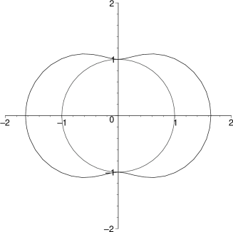
Figure 1: Polar plot of the locus of the horizon (inner circle) and ergosurface (outer deformed circle) of the stringy Kerr-Taub-NUT spacetime. The radial direction is $\sqrt{|x|}$, and the angle $\theta$ runs from $0$ at the north pole (N) to $\pi$ at the south pole (S). (This plot is for $\tau=2.5$.)

To see that the ergosphere really is a region where particles cannot be stationary, consider the following. Assume that a particle follows a trajectory with tangent vector $u$, which has to be timelike i.e., $u^{2}<0$. In the stationary case, the only motion is in the time direction, so the tangent vector is $u=u^{t}\frac{\partial}{\partial t}$, where $u^{t}=\frac{dt}{ds}$, and $s$ is proper time along the curve. But this gives $u^{2}=G_{tt}(u^{t})^{2}>0$ in the ergosphere (where $G_{tt}>0$), and so the assumptions are inconsistent: No stationary motion is possible in the ergosphere. What happens instead is that particles are affected by the rotational frame dragging and inevitably follow the rotation of the black hole (as observed from infinity) [22].

Note that both the Killing horizons and the ergosurface are independent of $k$, and are therefore not not modified by the high-energy corrections of the spacetime.

4.1.1 Curvature singularities

The metric (21) is ill defined for $D(x,\theta)=0$, which is also a true curvature singularity. This can be verified by computing the curvature. It is then seen that both the Ricci scalar and the Kretschmann scalar ($R^{\mu\nu\rho\sigma}R_{\mu\nu\rho\sigma}$) behave like $\sim\frac{1}{D(x,\theta)^{2}}$, and so indeed $D=0$ represents a curvature singularity. (The same argument would also show that $x^{2}-1=0$ or $E=0$ are not curvature singularities.)

First of all, notice that $D=0$ only has solutions if

$$x^{2}-1-\tau^{2}\sin^{2}\!\theta=E(x,\theta)>0,$$ (29)

that is, singularities are only found outside the ergosphere. (Inside the ergosurface, $D$ is always positive.) The equation $D(x,\theta)=0$ solved for $x$ gives

$$\begin{split}x=x_{\pm}(\theta)=&-\frac{1}{k-2}(\beta\mp\sqrt{\alpha^{2}}),\\ &\alpha^{2}=4(k+2)(\delta-\lambda\tau\cos\theta)^{2}-4(k-2)(1+\tau^{2}\sin^{2}\!\theta),\\ &\beta=(k+2)(\delta-\lambda\tau\cos\theta).\end{split}$$ (30)

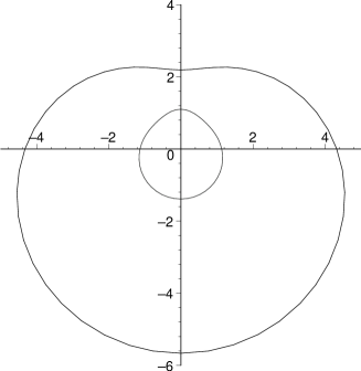
$x<0$ domain

Figure 2: Polar plots of the locus of the singularities for the small $\tau$ case. The radial direction is $\sqrt{|x|}$, and the angle $\theta$ is zero at the north pole (N) and $\pi$ at the south pole (S). There is symmetry in the $\phi$ direction. (This plot is for $k=3,\delta=2,\lambda=14,\tau=0.1$.)

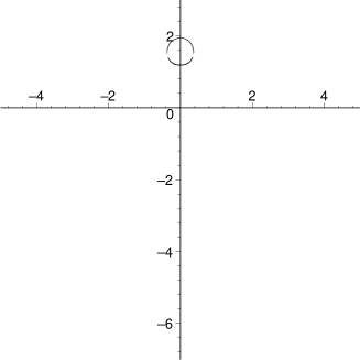
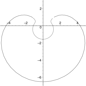
$x>0$ domain		$x<0$ domain

Figure 3: Polar plots of the locus of the singularities for the large $\tau$ case. (This plot is for $k=3,\delta=2,\lambda=14,\tau=0.18$.)

For given values of the parameters and for $\theta$, the solutions $x_{\pm}$ have the same sign (which is the same sign as $-\beta$), as can easily be seen from the following:

$$\beta^{2}-\alpha^{2}=(k+2)(k-2)(\delta-\lambda\tau\cos\theta)^{2}+4(k-2)(1+\sin^{2}\!\theta)\geq 0.$$ (31)

Hence, $|\beta|\geq|\alpha|$.

The singularities $x_{\pm}(\theta)$ can be divided into two classes, depending on the values of the parameters $k,\lambda,\delta,\tau$. Assuming $k,\delta,\lambda$ are given, there is a critical value for $\tau$ above which $\alpha^{2}$ in equation (30) is not positive definite. Call this critical value $\tau_{c}(k,\delta,\lambda)$. Then “small rotation” means values $\tau<\tau_{c}$, and “large rotation” means values $\tau>\tau_{c}$.

The first class is the small rotation case, where $\tau<\tau_{c}$. In this case $\alpha^{2}$ is always positive, and $x_{\pm}$ exist for all $\theta$, and are both negative. This situation is illustrated in figure 2. The spacetime structure in this case is a smooth deformation of the non-rotating stringy Taub-NUT spacetime discussed in ref.[1], with the same essential features. The singularities appear in the negative $x$ region, and enclose a region of Euclidean signature. Seen from the positive $x>1$ NUT region, and the from the Taub region $-1<x<1$ this is a singularity hidden behind a horizon, while from the negative $x<-1$ NUT regions they appear as naked singularities.

The second class is the large rotation case, where $\tau>\tau_{c}$. In this case, $\alpha^{2}$ becomes negative for some values of $\theta$. Hence, for these angles, there are no divergences. This is illustrated in figure 3. What happens is that the two surfaces $x\pm(\theta)$ connect and form a “bubble” outside the ergosphere. One such bubble is centred at the south pole ($\theta=\pi$) and appear in the negative $x$ region. This also makes the two NUT regions in the negative $x$ domain merge together into one connected region. Another bubble may or may not appear at the north pole ($\theta=0$) for positive $x$. This is rather different from the non-rotating case, and quite exotic behaviour. The bubbles still enclose regions of Euclidean signature, but since they appear in both the positive and the negative $x$ region, all the NUT regions are plagued by naked singularities.

5 Discussion

The model discussed in this paper is a generalisation of the stringy Taub-NUT spacetime of ref.[1]. The rotational symmetry is broken in the general case. It was demonstrated in that earlier work that the $\alpha^{\prime}$ corrections do not modify the spacetime significantly with regards to the CTCs in the non-rotating case, and this result persists in the rotating case. So all the comments made there carry on to the more general model of this paper. This is a valuable observation in that it shows us that the results of ref.[1] are not simply a coincidence happening only for that particular spacetime. Noting the miraculous cancellation that gave the simple form for the exact metric, we could have been tempted to believe there was something very special happening in that case. Now, as we see the same happening again, an interpretation of it as a mere coincidence seems even more unlikely. A more reasonable interpretation of the mild $\alpha^{\prime}$ corrections near the horizons seems to be that string theory really does not rule out the possibility of CTCs. This view has already been discussed in ref.[1].

The above comments are closely related to the observations that the horizons and the ergosurface are not modified by the high-energy corrections of the spacetime.

The curvature singularities in the present model differ from what we saw in the non-rotating case, and this deserves a comment. First of all, it is important to keep in mind that the dilaton blows up at the singularity, so the string coupling $g_{s}$ is in no sense small. Hence, $g_{s}$ corrections may completely alter the geometry at the “would-be-singularities” where $D(x,\theta)=0$. How to compute these corrections, however, is beyond reach with our technology at present. So the exotic singular structure of the metric (21) might only be an artifact of working in the classical limit (which is a good approximation only if $g_{s}\to 0$).

If we ignore this for a moment, we have spacetimes containing problematic naked singularities in the NUT regions. If the rotation is small, these appear only for negative $x$, and so we could still make sense of the positive $x$ NUT region since it would be protected from the singularities by the horizons at $x=\pm 1$. In this case the Taub region has a natural extension past $x=1$ into the region $x>1$, giving a cosmology with a post Big Crunch scenario. If the rotation is large, on the other hand, the singularities appear both in the positive and negative $x$ NUT regions, and any sensible extension of the Taub region seems impossible.

References

- [1] C. V. Johnson and H. G. Svendsen, An exact string theory model of closed time-like curves and cosmological singularities, hep-th/0405141. Submitted to Phys. Rev. D.
- [2] A. H. Taub, Empty space-times admitting a three parameter group of motions, Annals Math. 53 (1951) 472–490.
- [3] E. Newman, L. Tamubrino and T. Unti, Empty space generalization of the schwarzschild metric, J. Math. Phys. 4 (1963) 915.
- [4] C. V. Johnson and R. C. Myers, A conformal field theory of a rotating dyon, Phys. Rev. D52 (1995) 2294–2312 [hep-th/9503027].
- [5] C. V. Johnson, Heterotic coset models, Mod. Phys. Lett. A10 (1995) 549–560 [hep-th/9409062].
- [6] C. V. Johnson, Exact models of extremal dyonic 4-D black hole solutions of heterotic string theory, Phys. Rev. D50 (1994) 4032–4050 [hep-th/9403192].
- [7] D. V. Galtsov and O. V. Kechkin, Ehlers-harrison type transformations in dilaton - axion gravity, Phys. Rev. D50 (1994) 7394–7399 [hep-th/9407155].
- [8] C. V. Johnson and R. C. Myers, Taub–NUT dyons in heterotic string theory, Phys. Rev. D50 (1994) 6512–6518 [hep-th/9406069].
- [9] R. Kallosh, D. Kastor, T. Ortin and T. Torma, Supersymmetry and stationary solutions in dilaton axion gravity, Phys. Rev. D50 (1994) 6374–6384 [hep-th/9406059].
- [10] E. Witten, On holomorphic factorization of WZW and coset models, Commun. Math. Phys. 144 (1992) 189–212.
- [11] W. A. Hiscock and D. A. Konkowski, Quantum vacuum energy in taub - nut (newman-unti-tamburino) type cosmologies, Phys. Rev. D26 (1982) 1225–1230.
- [12] E. Witten, On string theory and black holes, Phys. Rev. D44 (1991) 314–324.
- [13] R. Dijkgraaf, H. Verlinde and E. Verlinde, String propagation in a black hole geometry, Nucl. Phys. B371 (1992) 269–314.
- [14] A. A. Tseytlin, On the form of the black hole solution in d = 2 theory, Phys. Lett. B268 (1991) 175–178.
- [15] I. Jack, D. R. T. Jones and J. Panvel, Exact bosonic and supersymmetric string black hole solutions, Nucl. Phys. B393 (1993) 95–110 [hep-th/9201039].
- [16] I. Bars and K. Sfetsos, Conformally exact metric and dilaton in string theory on curved space-time, Phys. Rev. D46 (1992) 4510–4519 [hep-th/9206006].
- [17] I. Bars and K. Sfetsos, string model in curved space-time and exact conformal results, Phys. Lett. B301 (1993) 183–190 [hep-th/9208001].
- [18] A. A. Tseytlin, Effective action of gauged wzw model and exact string solutions, Nucl. Phys. B399 (1993) 601–622 [hep-th/9301015].
- [19] I. Bars and K. Sfetsos, Exact effective action and space-time geometry in gauged WZW models, Phys. Rev. D48 (1993) 844–852 [hep-th/9301047].
- [20] H. Leutwyler and M. A. Shifman, Perturbation theory in the wess-zumino-novikov-witten model, Int. J. Mod. Phys. A7 (1992) 795–842.
- [21] M. A. Shifman, Four-dimension aspect of the perturbative renormalization in three-dimensional chern-simons theory, Nucl. Phys. B352 (1991) 87–112.
- [22] R. M. Wald, General Relativity. Chicago, USA: Univ. Pr., 1984. 491 p.