Yang–Mills sphalerons in all even spacetime dimensions $d=2k$, $k>2$ : $k$=3,4

Abstract

The classical solutions to higher dimensional Yang–Mills (YM) systems, which form part of higher dimensional Einstein–YM (EYM) systems, are studied. These are the gravity decoupling limits of the fully gravitating EYM solutions. In odd spacetime dimensions, depending on the choice of gauge group and its representation, these are either topologically stable or are unstable. Both cases are analysed, the latter numerically only. In even spacetime dimensions they are always unstable, describing saddle points of the energy, and can be described as sphalerons. This instability is analysed by constructing the noncontractible loops and calculating the Chern–Simons (CS) charges, and also perturbatively by numerically constructing the negative modes. This study is restricted to the simplest YM system in spacetime dimensions $d=6,7,8$, which captures the qualitative features of the generic case.

1 Introduction

Gravitational and non Abelian gauge fields occur in low energy effective actions [1] of superstring theory and supergravities. On the other hand classical solutions to the Einstein–Yang-Mills (EYM) system, especially black holes, have an important role to play in quantum gravity [2]. These effective actions consist, in addition to the usual Einstein-Hilbert and Yang–Mills (YM) systems, of higher order terms in both the gravitational curvature, and the YM curvature and its gauge covariant derivatives. Moreover some of the theories in which such terms are present are defined in higher dimensional spacetimes, namely on $D$-branes [3]. Thus, the study of classical solutions to higher curvature EYM models in higher dimensions is of physical interest.

It turns out that in higher (than $3+1$) dimensions, the higher order YM curvature terms play a much more important role than do the corresponding gravitational terms, e.g. Gauss-Bonnet terms. Inclusion of the latter does not seem to alter the qualitative properties of the classical solutions, while the absence of higher order YM terms prevents the existence of such solutions due to the Derrick scaling requirements not being satisfied. It is for this reason that we restrict our considerations in this paper to the inclusion of higher order YM  only. Our aim being the study of the stability (and its absence) in these systems, we ignore the gravitational terms entirely since the most important mechanism affecting stability/instability is characterised by the YM sector alone.

Concerning the higher order YM curvature terms in the string theory effective action, the situation is complex and as yet unresolved. While YM terms up to $F^{4}$ arise from (the non Abelian version of) the Born–Infeld action [5], it appears that this approach does not yield all the $F^{6}$ terms [6]. Terms of order $F^{6}$ and higher can also be obtained by employing the constraints of (maximal) supersymmetry [7]. The results of the various approaches are not identical.

Given the evolving stage which higher order curvature YM terms are in, and motivated by the technical requirements for the construction of classical solutions, we have restricted our considerations to one particular family of higher curvature YM systems. The criterion is that only the second power (and no higher power) of the velocity field $\partial_{0}A_{i}$ occur in the Lagrangian. This constrains our choice to one where the coefficients of each $F^{2n}$ term is fixed by the requirement that only totally antisymmetrised curvature $n$-forms are employed. We have no physical justification for this, but we hope that the ensuing qualitative results hold also in the more general, and as yet not definitely fixed, cases. In this family of YM systems the number of higher order terms that can arise in any given dimension is limited due to the imposed antisymmetry.

The other constraint we apply is that in any given dimension, we truncate the series of $F^{2n}$ terms, to the minimum required to satisfy the Derrick scaling requirement. Our justification here is that higher order terms become more important at high energies so in the low energy effective action it is sufficient to keep the lowest order terms.

It is well known that there exist static regular [8] and black hole[9, 10] solutions to the Einstein–Yang-Mills (EYM) system in $d=4$ spacetime dimensions. To construct static solutions to gravitating Yang–Mills (YM) systems in spacetime dimensions $d\geq 5$ [11, 12], terms of higher order in the YM curvature must be included. Such terms appear in various low energy effective actions of string theory. For our practical purposes, a particulary useful family of such YM systems is

$${\cal L}_{P}=\sum_{p=1}^{P}\frac{\tau_{p}}{2(2p)!}\ \mbox{Tr}\,F(2p)^{2}$$ (1)

which is the sum of the terms in the YM hierarchy [13], with $F(2p)$ being the $p$ fold totally antisymmetrised products of the YM curvature, $F(2)=F_{\mu\nu}$, in this notation. Clearly, the highest value $P$ of $p$ in (1) is finite and depends on the dimensionality $d$ of the spacetime. In [11, 12] we chose the simplest possibility $P=2$, since we restricted our study to $8\geq d\geq 5$. The study of the classical solutions to the systems (1), which turn out to be the gravity–decoupling solutions of EYM systems in these dimensions, is the aim of this paper. This is an important aspect of the study of higher dimensional EYM solutions.

To complete the definition of the models (1) the gauge group $G$ must be specified. With the aim of constructing static spherically symmetric solutions in $d$ spacetime dimensions, the smallest such gauge group is $G=SO(d-1)$ . Static finite energy solutions to the systems (1) may or may not be topologically stable depending on the dimensionality $d$ of the spacetime and the choice of gauge group $G$.

The purpose of the present work is to resolve the question of stability or instability of these spherically symmetric solutions quantitatively. These are the gravity decoupling limits of the static and regular solutions to EYM systems in spacetime dimensions $d\geq 6$ [11]. In the $d=5$ case [12], as in the usual $d=4$ case [8], there are no gravity decoupling solutions, unlike in the case of the EYM-Higgs (EYMH) systems in $d=4$ whose regular solutions [14, 15] tend to the ’t Hooft-Polyakov monopole in the flat space limit. In both cases, higher dimensional EYM and EYMH in $d=4$, the models feature an additional dimensional constant. As a result gravitating solutions exist only for a finite range of values of the gravitational constant. Here, we restrict to the non–gravitating models only.

For simplicity, we restrict to the model considered in [11], (1) with $p=1$ and $2$ only, in spacetime dimensions $d=6,7$ and $8$. Solutions to this model on $d=6$ Euclidean space were constructed in [16] in a different context. Consistently with our requirement for the imposition of spherical symmetry we choose $G=SO(d-1)$ and $G=SO(d)$, and because of the higher order of nonlinearity in the $p>1$ models the choice of the concrete representations of $G$ is important.

Except for the case where there exists a nonvanishing Chern–Pontryagin (CP) charge in the spacelike dimensions, these solutions are unstable. In the particular cases where $G$ and its representation is chosen such that the Chern–Simons (CS) charge is nonzero, this instability will be that of a sphaleron [17, 18]. The quantitative study [19] of the latter will be the major task below.

In section 2, we present the detailed models and the corresponding CS densities. In section 3, spherical symmetry in the $d-1$ spacelike dimensions is imposed and the residual one dimensional models are displayed in 3.1 where the gauge invariance of the Ansatz is also stated. The static equations are given in 3.2 and the corresponding CS densities in 3.3. In 3.4, the CS charges are calculated. Section 4 contains our numerical results. In 4.1 we have constructed the noncontractible loop (NCL) for the unstable solutions and have plotted the energy of the solution versus the angle parametrising this loop. In those cases where there is a nonvanishing CS charge, the energy is plotted also against the CS number. In 4.2 we have constructed the negative modes excited by the instability and have calculated the negative eigenvalues. Section 5 is devoted to a summary and discussion of our results.

2 The models and Chern-Simons densities

In the first subsection 2.1 we define the static energy density functional resulting from the Lagrangian (1) in spacetime dimensions $d=6,7,8$, and consider the topological lower bound on the energy for the $d=7$ case. In the second subsection 2.2 we define the Chern-Simons densities for the models in spacetimes $d=6$ and $8$.

Spacetime coordinates are labeled by Greek indices $\mu,\nu,...$, and spacelike coordinates by Latin indices $i,j,k,...$.

2.1 The models

Since we are interested in static solutions, we will define the models on the $d-1$ dimensional Euclidean spacelike manifold. In the present work, we will restrict our considerations to the $P=2$ model (1) used in [11]. Expressed in component form this is

$${\cal H}_{2}=-\frac{\tau_{1}}{2.2!}\,\mbox{Tr}\,F_{ij}^{2}\,+\,\frac{\tau_{2}}{2.4!}\,\mbox{Tr}\,F_{ijkl}^{2}$$ (2)

where

$$F_{ijkl}\,=\,\{F_{i[j},F_{kl]}\}$$

is the $4$-form curvature, and $[jkl]$ implies cyclic symmetrisation. In the light of Derrick’s scaling requirement, (2) is the simplest model that can support static finite energy solutions for spacetime dimensions up to $d=8$. Beyond that terms with higher values $p$ must be included in (1), but this is entirely unnecessary since all our conclusions from the present investigation hold qualitatively also for $d\geq 9$.

The model is specified finally by the choice of the gauge group $G$, as well as its representaion. We will mostly restrict ourselves to $G=SO(d)$, but for odd $d$ we will include the special case of $G=SO(d-1)$ as well.

When $d$ is even, i.e. $d=6$ and $8$ in our examples, there exists a Chern–Simons (CS) density in the $5$ and $7$ spacelike dimensions and the static solutions will display a sphaleron like unstability. As will be seen below, the nonvanishing of the CS density is what necessitates the choice of $G=SO(d)$, with $d=6$ and $8$. These two examples will be the main focus of our attention.

When $d$ is odd, i.e. $d=7$ in our examples, there exists a Chern-Pontryagin (CP) density in the $6$ spacelike dimensions. Provided that $G$ and its representation is chosen suitably, this CP density is nonvanishing and the resulting static solution will be stable. As will be seen below, the existence of a stable soltion is what necessitates the choice of $G=SO(6)(=SO(d-1))$ here. Otherwise, with $G=SO(7)(=SO(d))$, the static solution will not be stable.

Before proceeding to state the CP and the CS densities for the even $d$ systems, we give the topological lower bound on the energy density functional of the odd $d$, namely the $d=7$ system. The inequality

$$\mbox{Tr}\left(\sqrt{\tau_{1}}F_{ij}-\frac{\sqrt{\tau_{2}}}{4!}\varepsilon_{ijklmn}F_{klmn}\right)^{2}\geq 0$$ (3)

leads to

$${\cal H}_{2}\geq\frac{1}{8}\sqrt{\tau_{1}\tau_{2}}\,\varepsilon_{ijklmn}\,\mbox{Tr}\,F_{ij}F_{kl}F_{mn}\,,$$ (4)

stating the topological lower bound in terms of the 3rd CP desity. It follows that the spherically symmetric solution [16] to the model in $d=7$ is topologically stable provided that the CP density on the right hand side does not vanish. This is the case for $G=SO(d-1)=SO(6)$, but only if the gauge fields are in the chiral represenation of $G$. These static solutions in even spacelike dimensions, which obey instanton like boundary conditions, play the role of solitons. The topological inequality (3) cannot be saturated since the corresponding Bogomol’nyi equations are overdetermined.

2.2 The Chern-Pontryagin and Chern-Simons densities

The definition of Chern-Simons (CS) densities in $d-1$ spacelike dimensions follows from that of the Chern-Pontryagin (CP) densities, in even spacetime dimensions,

$$\varrho_{d}=\frac{1}{N_{d}}\varepsilon_{\mu_{1}\mu_{2}\mu_{3}...\mu_{d}}\mbox{Tr}\,F_{\mu_{1}\mu_{2}}F_{\mu_{2}\mu_{3}}...F_{\mu_{d-1}\mu_{d}}\quad,\quad d=6\quad{\rm and}\quad d=8\,,$$ (5)

where $N_{d}$ is the appropriate normalisation factor for dimension $d$. Of course, for the purpose of definition (5), the signature is taken to be Euclidean.

The CP density is a total divergence, which we denote generally as

$$\varrho_{d}=\partial_{\mu}\,\Omega_{\mu}^{(d)}\,.$$ (6)

In the two cases of interest at hand, with $d=6$ and $d=8$, $\Omega_{\mu}^{(d)}$ is given by

$$\Omega_{\mu_{1}}^{(6)} = \frac{5}{2^{6}\cdot\pi^{3}}\varepsilon_{\mu_{1}\mu_{2}\mu_{3}...\mu_{6}}\mbox{Tr}\,A_{\mu_{2}}\left[F_{\mu_{3}\mu_{4}}F_{\mu_{5}\mu_{6}}-F_{\mu_{3}\mu_{4}}A_{\mu_{5}}A_{\mu_{6}}+\frac{2}{5}A_{\mu_{3}}A_{\mu_{4}}A_{\mu_{5}}A_{\mu_{6}}\right]$$ (7)

$$\Omega_{\mu_{1}}^{(8)} = \frac{7}{3\cdot 2^{12}\cdot\pi^{4}}\varepsilon_{\mu_{1}\mu_{2}\mu_{3}...\mu_{8}}\mbox{Tr}\,A_{\mu_{2}}\bigg{[}F_{\mu_{3}\mu_{4}}F_{\mu_{5}\mu_{6}}F_{\mu_{7}\mu_{8}}-\frac{4}{5}F_{\mu_{3}\mu_{4}}F_{\mu_{5}\mu_{6}}A_{\mu_{7}}A_{\mu_{8}}-\frac{2}{5}F_{\mu_{3}\mu_{4}}A_{\mu_{5}}F_{\mu_{6}\mu_{7}}A_{\mu_{8}}$$ (8)

$$\qquad\qquad\qquad\qquad\qquad\qquad+\frac{4}{5}F_{\mu_{3}\mu_{4}}A_{\mu_{5}}A_{\mu_{6}}A_{\mu_{7}}A_{\mu_{8}}-\frac{8}{35}A_{\mu_{3}}A_{\mu_{4}}A_{\mu_{5}}A_{\mu_{6}}A_{\mu_{7}}A_{\mu_{8}}\bigg{]}\,.$$

From (7) and (8), the respective CS densities $\nu_{d-1}$ are defined to be the $\mu=0$ components of $\Omega_{\mu}^{(d)}$ in $5$ and $7$ Euclidean spacelike dimensions

$$\nu_{5} = -\frac{5}{2^{6}\cdot\pi^{3}}\varepsilon_{i_{1}i_{2}i_{3}...i_{5}}\mbox{Tr}\,A_{i_{1}}\left[F_{i_{2}i_{3}}F_{i_{4}i_{5}}-F_{i_{2}i_{3}}A_{i_{4}}A_{i_{5}}+\frac{2}{5}A_{i_{2}}A_{i_{3}}A_{i_{4}}A_{i_{5}}\right]$$ (9)

$$\nu_{7} = -\frac{7}{3\cdot 2^{12}\cdot\pi^{4}}\varepsilon_{i_{1}i_{2}i_{3}...i_{7}}\mbox{Tr}\,A_{i_{1}}\bigg{[}F_{i_{2}i_{3}}F_{i_{4}i_{5}}F_{i_{6}i_{7}}-\frac{4}{5}F_{i_{2}i_{3}}F_{i_{4}i_{5}}A_{i_{6}}A_{i_{7}}-\frac{2}{5}F_{i_{2}i_{3}}A_{i_{4}}F_{i_{5}i_{6}}A_{i_{7}}$$ (10)

$$\qquad\qquad\qquad\qquad\qquad\qquad+\frac{4}{5}F_{i_{2}i_{3}}A_{i_{4}}A_{i_{5}}A_{i_{6}}A_{i_{7}}-\frac{8}{35}A_{i_{2}}A_{i_{3}}A_{i_{4}}A_{i_{5}}A_{i_{6}}A_{i_{7}}\bigg{]}\,.$$

3 Imposition of spherical symmetry

Our choice of gauge group will be $G=SO(d)$, except in $d=7$ where we will consider and dispose of the special case $G=SO(6)=SO(d-1)$. Our choice of $G=SO(d)$ for even $d$ is similar to the choice for the Weinberg–Salam [17] (WS) and for the Bartnik–McKinnon [21, 22] sphalerons in $d=4$. Furthermore, like in the latter case, we will employ the chiral representation $G=SO_{\pm}(d)$, noting that for the special case $d=4$, $G=SO_{\pm}(4)=SU_{L/R}(2)$.

Since our main aim is to study the instability of the solutions to (2), we will employ the general spherically symmetric Ansatz parametrised by three radial functions $w_{1}(r)$, $w_{2}(r)$ and $w_{3}(r)$. This follows from the axially symmetric Ansatz [20] in $d$ dimensions where all the components of the gauge connection are taken to be independent of $x_{0}$ and the component $A_{0}=0$. Like the sphalerons [17, 22] in $d=4$, our solutions are also parametrised by the function $w_{1}$ while the functions $(w_{2},w_{3})$ will be excited only in the directions of the instability.

For even $d$ with $G=SO(d)$, including $d=4$, the imposition of spherical symmetry on the gauge field on $(d-1)$ dimensional Euclidean space results in

$$A_{i}=\frac{1-w_{1}(r)}{r}\ \Sigma_{ij}^{(d)}\,\hat{x}_{j}+\frac{w_{2}(r)}{r}\,(\delta_{ij}-\hat{x}_{i}\hat{x}_{j})\,\Sigma_{j,d}^{(d)}+\frac{w_{3}(r)}{r}\,\hat{x}_{i}\hat{x}_{j}\,\Sigma_{j,d}^{(d)}$$ (11)

where $\Sigma_{ij}^{(d)}$ is (one of) the chiral representaion(s) of the algebra of $SO(d)$, namely

$$\Sigma_{ij}^{(d)} = \left(\frac{1{\rm I}\pm\Gamma_{d+1}}{2}\right)\Gamma_{ij}$$ (12)

$$\Gamma_{ij}^{(d)} = -\frac{1}{4}[\Gamma_{i},\Gamma_{j}]\,,$$ (13)

$\Gamma_{ij}$ being the spinor represention matrices of the algebra of $SO(d)$ defined in terms of $\Gamma_{i}$, the gamma matrices in $d$ dimensions.

For odd $d$ with $G=SO(d)$, there are no chiral representations, so the Ansatz (11) holds only in a formal way, replacing the matrices $\Sigma_{ij}^{(d)}$ by $\Gamma_{ij}^{(d)}$.

For odd $d$ with $G=SO(d)$, it is possible to employ the chiral representation of $SO(d-1)$. Here again, (11) holds formally, but now by replacing $d$ with $d-1$ in it. As noted above, in this case the solution (with $w_{2}=w_{3}=0$ everywhere) will describe a stable soliton.

For the evaluation of the residual one dimensional energy density functional, only the algebraic properties of $\Sigma_{ij}^{(d)}$ and of $\Gamma_{ij}^{(d)}$ enter the calculations, so the same result holds (up to an unimportant numerical factor $2$) both for even and for odd $d$ and with all $G$. For the evaluation of the CP and CS densities however, this distinction must be kept.

3.1 Reduced one dimensional systems and gauge freedom

Imposition of spherical symmetry on the $(d-1)$ dimensional $SO(d)$ system results in the one dimensional energy density functional

$$H_{d} = \frac{2^{\frac{d-2}{2}}\tau_{1}}{2\cdot 2!}\,\frac{d-2}{4}\,r^{d-4}\cdot\left[\left(w_{1}^{\prime}+\frac{w_{2}w_{3}}{r}\right)^{2}+\left(w_{2}^{\prime}-\frac{w_{1}w_{3}}{r}\right)^{2}+\frac{d-3}{2r^{2}}(1-|\vec{w}|^{2})^{2}\right]$$ (14)

$$+ \frac{2^{\frac{d-2}{2}}\tau_{2}}{2\cdot 4!}\,3^{2}\,(d-2)(d-3)(d-4)\,r^{d-8}(1-|\vec{w}|^{2})^{2}\cdot$$

$$\qquad\qquad\cdot\left[\left(w_{1}^{\prime}+\frac{w_{2}w_{3}}{r}\right)^{2}+\left(w_{2}^{\prime}-\frac{w_{1}w_{3}}{r}\right)^{2}+\frac{d-5}{4r^{2}}(1-|\vec{w}|^{2})^{2}\right]\,,$$

in which we have used the shorthand notation

$$|\vec{w}|^{2}=w_{1}^{2}+w_{2}^{2}\,.$$

For odd $d=7$ and with $G=SO(6)$, (14) holds as well, but the solutions to the field equations (to be presented in the following subsection) are quite different, with $w_{1}=w_{2}=0$ everywhere.

In the generic case, for the fields (11), the requirement of analyticity at the origin $r=0$ results in the asymptotic conditions

$$w_{1}(0)=1\quad,\quad w_{2}(0)=0\quad,\quad w_{3}(0)=0\,,$$ (15)

while in the asymptotic region $r\gg 1$ the requirement of finiteness of the energy results in the boundary condition

$$\lim_{r\rightarrow\infty}|\vec{w}|^{2}=\lim_{r\rightarrow\infty}(w_{1}^{2}+w_{2}^{2})^{2}=1\,.$$ (16)

(16) can be parametrised, like in [19], in terms of the familiar angle $q$ as

$$\lim_{r\rightarrow\infty}w_{1}=\cos q\quad,\quad\lim_{r\rightarrow\infty}w_{2}=\sin q\,.$$ (17)

The conditions (16)-(17) can be understood better by displaying the gauge freedom of the energy density functional (14), under the action of the local $U(1)$ transformation

$$g[\omega(r)]\in U(1)\quad,\quad\lim_{r\to 0}\omega(r)=0\quad,\quad\lim_{r\to\infty}\omega(r)=-q\,.$$ (18)

The action of this $U(1)$ gauge transformation is given by

$$\left(\begin{array}[]{c}w_{1}\\ w_{2}\end{array}\right) \stackrel{{\scriptstyle g[\omega]}}{{\mapsto}} \left(\begin{array}[]{cc}\cos\omega&-\sin\omega\\ \sin\omega&\cos\omega\end{array}\right)\left(\begin{array}[]{c}w_{1}\\ w_{2}\end{array}\right)$$ (25)

$$w_{3} \stackrel{{\scriptstyle g[\omega]}}{{\mapsto}} w_{3}+r\,\omega^{\prime}\,.$$ (26)

3.2 The Euler–Lagrange equations

The Euler-Lagrange equations of the $SO(d)$ systems are, for variations of $w_{1}$, $w_{2}$ and $w_{3}$ in that order,

$$\tau_{1} \left\{w_{1}^{\prime\prime}+\frac{1}{r}[(d-4)w_{1}^{\prime}+2w_{2}^{\prime}w_{3}+w_{2}w_{3}^{\prime}]+\frac{1}{r^{2}}\left([(d-3)(1-|\vec{w}|^{2})-w_{3}^{2}]w_{1}+(d-5)w_{2}w_{3}\right)\right\}$$ (27)

$$+ \ \frac{3\tau_{2}}{4r^{4}}(d-3)(d-4)\ (1-|\vec{w}|^{2})\cdot$$

$$\bigg{\{}(1-|\vec{w}|^{2})\left(w_{1}^{\prime\prime}+\frac{1}{r}[(d-8)w_{1}^{\prime}+2w_{2}^{\prime}w_{3}+w_{2}w_{3}^{\prime}]+\frac{1}{r^{2}}\left([(d-5)(1-|\vec{w}|^{2})-w_{3}^{2}]w_{1}+(d-9)w_{2}w_{3}\right)\right)$$

$$+ 2\left[\left(w_{1}^{\prime}+\frac{w_{2}w_{3}}{r}\right)^{2}+\left(w_{2}^{\prime}-\frac{w_{1}w_{3}}{r}\right)^{2}\right]w_{1}-2\left(|\vec{w}|^{2}\right)^{\prime}\left(w_{1}^{\prime}+\frac{w_{2}w_{3}}{r}\right)\bigg{\}}=0$$

$$\tau_{1} \left\{w_{2}^{\prime\prime}+\frac{1}{r}[(d-4)w_{2}^{\prime}-2w_{1}^{\prime}w_{3}-w_{1}w_{3}^{\prime}]+\frac{1}{r^{2}}\left([(d-3)(1-|\vec{w}|^{2})-w_{3}^{2}]w_{2}-(d-5)w_{1}w_{3}\right)\right\}$$ (28)

$$+ \ \frac{3\tau_{2}}{4r^{4}}(d-3)(d-4)\ (1-|\vec{w}|^{2})\cdot$$

$$\cdot \bigg{\{}(1-|\vec{w}|^{2})\left(w_{2}^{\prime\prime}+\frac{1}{r}[(d-8)w_{2}^{\prime}-2w_{1}^{\prime}w_{3}-w_{1}w_{3}^{\prime}]+\frac{1}{r^{2}}\left([(d-5)(1-|\vec{w}|^{2})-w_{3}^{2}]w_{2}-(d-9)w_{1}w_{3}\right)\right)$$

$$+ 2\left[\left(w_{1}^{\prime}+\frac{w_{2}w_{3}}{r}\right)^{2}+\left(w_{2}^{\prime}-\frac{w_{1}w_{3}}{r}\right)^{2}\right]w_{2}-2\left(|\vec{w}|^{2}\right)^{\prime}\left(w_{2}^{\prime}-\frac{w_{1}w_{3}}{r}\right)\bigg{\}}=0$$

$$\left[\tau_{1}+\frac{3\tau_{2}}{4r^{4}}(d-3)(d-4)(1-|\vec{w}|^{2})^{2}\right]\left[(w_{1}w_{2}^{\prime}-w_{2}w_{1}^{\prime})-\frac{1}{r}w_{3}|\vec{w}|^{2}\right]=0\ .\qquad\qquad\qquad$$ (29)

The last equation, (29), is satisfied by the solutions of (27) and (28), as can be seen straighforwardly by differentiating (29) and identifying it with the difference of $w_{2}$ times (27) and $w_{1}$ times (28). Thus, exploiting the gauge freedom (25)-(26), we choose the radial gauge with $w_{3}=0$. We then proceed to solve the two equations (27) and (28) for the two functions $w_{1}$ and $w_{2}$.

We note here that in the $w_{3}=0$ gauge, equations (27) and (28) are symmetric in the functions $w_{1}$ and $w_{2}$ as in the case of the Bartnik-McKinnon sphaleron [21, 22], and in contrast to the WS case [19] in which this symmetry is absent due to the presence of the complex doublet Higgs field.

3.2.1 $SO_{\pm}(d-1)$ solitons in $d$ dimensions

Before proceeding to consider the sphaleron solutions, we dispose of the stable soliton solutions of the models in odd $d$ spacetime dimensions when the gauge connection takes its values in the chiral representation of $SO(d-1)$. We restrict this demonstration to the model in $d=7$, with $G=SO_{\pm}(6)$.

As a practical illustration of the topological lower bound (4), using the notation $\kappa_{1}=\sqrt{(d-2)\tau_{1}/2}$, $\kappa_{2}=3\sqrt{(d-2)(d-3)(d-4)\tau_{2}}$, consider the two inequalities

$$\left[\kappa_{1}r^{\frac{d-4}{2}}w^{\prime}-\kappa_{2}r^{\frac{d-8}{2}}\sqrt{\frac{d-5}{4r^{2}}}(1-w^{2})^{2}\right]^{2} \geq 0$$ (30)

$$\left[\kappa_{2}r^{\frac{d-8}{2}}(1-w^{2})w^{\prime}-\kappa_{1}r^{\frac{d-4}{2}}\sqrt{\frac{d-3}{2r^{2}}}(1-w^{2})\right]^{2} \geq 0\ .$$ (31)

Adding (30) and (31) we have

$$H_{d}[w_{1},w_{2},w_{3}]=H_{d}[w,0,0]\geq 2\kappa_{1}\kappa_{2}\left(\sqrt{\frac{d-5}{4}}+\sqrt{\frac{d-3}{2}}\right)r^{d-7}\,(1-w^{2})\,w^{\prime}\ ,$$ (32)

where $H_{d}[w,0,0]$ is given by the energy density functional (14) with $w_{1}=w$ and $w_{2}=w_{3}=0$. It is now obvious that the right hand side of the inequality (32) is a total derivative only for the spacetime dimension $d=7$ at hand, and that it is the residual CP density after the imposition of spherical symmetry on the $G=SO_{\pm}(d-1)=SO_{\pm}(6)$ model, with $G$ is in the chiral representation.

3.3 Reduced Chern-Simons densities and non–contractible loop

The reduced one dimensional Chern-Simons (CS) densities of static gauge fields (11) in (even) $d$ spacetime dimensions, with gauge groups $G=SO(d)$ in the chiral representation $SO_{\pm}(d)$, take on nonvanishing values . The particular examples considered concretely here are those in $d=6$ and $d=8$, given by (9) and (10). Subjecting these to spherical symmetry according to the Ansatz (11), we find

$$n_{5} = -\frac{5}{2\pi}\left\{[2(1-w_{1})+3(1-|\vec{w}|^{2})][(w_{1}-1)w_{2}^{\prime}-w_{2}w_{1}^{\prime}]+\frac{3}{r}\,w_{3}\,(1-|\vec{w}|^{2})^{2}\right\}$$ (33)

$$n_{7} = -\frac{7}{5\cdot 2^{3}\pi}\bigg{\{}\left[5((1-w_{1})^{2}+w_{2}^{2})^{2}+6(1-w_{1})(3(1-w_{1})+4(1-|\vec{w}|^{2})]\right][(w_{1}-1)w_{2}^{\prime}-w_{2}w_{1}^{\prime}]$$ (34)

$$\qquad\qquad\qquad\qquad\qquad\qquad\qquad\qquad\qquad\qquad\qquad\ \ \,+\frac{5w_{3}}{r}(1-|\vec{w}|^{2})^{3}\bigg{\}}\,.$$

In what follows a most important role will be played by the non–contractible loop (NCL) of configurations displaying the instability of the sphalerons. In contrast to the case of the WS model [19], and similar to the Barnik–McKinnon sphaleron [21, 22]. This is a result of the $(w_{1},w_{2})$ symmetry in the field equations (27)-(28). In the former case where the doublet Higgs field removes this $(w_{1},w_{2})$ symmetry, conditional solutions with fixed CS number $Q_{CS}$ can be constructed by solving the equations of motion that extremise the energy density functional plus a Lagrange multiplier times the CS density. In the that case [19], the minimal finite energy path versus $Q_{CS}$ can be constructed concretely. The situation here is similar, rather, to the second case of the EYM sphaleron [21, 22], where the analysis of instability is carried out exclusively by employing a NCL.

The actual sphaleron solutions are parametrised by the functions

$$w_{1}=f(r)\quad,\quad w_{2}=0\quad,\quad w_{3}=0$$ (35)

which will be constructed numerically in the next section, consistently with the asymptotic conditions (15) and (16), the function $f(r)$ in (35) satisfies the asymptotics

$$\lim_{r\to 0}f(r)=1\quad,\quad\lim_{r\to\infty}f(r)=-1.$$ (36)

Following [23] we adopt the NCL configurations

$$\bar{w}_{1} = \frac{1}{2}(1+\cos q)+\frac{1}{2}(1-\cos q)\,f$$ (37)

$$\bar{w}_{2} = \frac{1}{2}(\sin q)\,(1-f)$$ (38)

$$\bar{w}_{3} = 0\,,$$ (39)

which by virtue of (36) ensures that both (15) and (17) are satisfied all along the NCL.

3.4 Calculation of the Chern–Simons number

In the case of the WS model [17, 18, 19, 22, 21], the CS number $Q_{CS}$ has the physical interpretation of Baryon number. Here, it merely is a convenient topological charge characterising the sphaleron.

The topological CP charges are are given by the $d$ dimensional volume integrals of $\partial_{\mu}\Omega_{\mu}^{(d)}$. Here we are interested in the $k=3$ and $k=4$ examples for which $\Omega_{\mu}^{(d)}$ are given by (7) and by (8) respectively, but now we consider static fields in a $d$ dimensional Minkowskian spacetime. The topologial charge in this context is referred to [18] as the CS charge $Q_{CS}$.

Adapting the arguments of [18] to our cases, notably assuming that $Q_{CS}=0$ at $t=-\infty$, the topological charges are given by

$$Q_{CS}=\frac{1}{N(d)}\left(\int_{-\infty}^{t_{0}}dt\int_{S_{(d-1)}}\Omega_{i}^{(d)}\ dS_{i}+\int_{t=t_{0}}d^{d-1}x\ \Omega_{0}^{(d)}\right)\,.$$ (40)

The Chern–Simons (CS) densities $\Omega_{0}^{(d)}=\nu_{d-1}$ are displayed by (9)-(10). The task at hand is to evaluate the integrals (40) for our two sphaleron solutions.

In the $w_{3}=0$ gauge in which the sphaleron solutions are constructed, the surface integral term in (40) does not vanish since the gauge potential decays with power $r^{-1}$ as $r\to\infty$, as seen from (11) and (35)-(36). It is convenient to evaluate (40) in a gauge in which the surface integral vanishes, such that

$$Q_{CS}=\frac{1}{N(d)}\int_{t=t_{0}}d^{d-1}x\ \Omega_{0}^{(d)}=\frac{1}{N(d)}\int_{t=t_{0}}\,\nu_{d-1}\,d^{d-1}x\,,$$ (41)

which for the spherically symmetric fields (11) reduces to the one dimensional integral

$$Q_{CS}=\int_{r=0}^{r=\infty}\,n_{d-1}\,dr\,$$ (42)

with $n_{d-1}(r)$ given by (33)-(34).

But substituting the NCL configuration (37)-(39) in the expressions for CS densities (33) and (34), results in the vanishing of $n_{5}$ and of $n_{7}$. This means that the nonvanishing contribution to the integral (40) must come from the surface integral term, which is not convenient to evaluate since the solutions and the NCL configurations at our disposal are time independent. But by definition (40) is gauge invariant, so it should be evaluated in a gauge in which the surface integral in (40) does not contribute. To this end, following [18], we subject (37)-(39) to the gauge transformation (25)-(26), such that

$$\lim_{r\to 0}\omega(r)=0\quad,\quad\lim_{r\to\infty}\omega(r)=-q\ .$$ (43)

With these boundary conditions on the $U(1)$ gauge group parameter, and (36) for the sphaleron profile function $f(r)$, we find

$$\lim_{r\to\infty}{}^{\omega}\bar{w_{1}}=1\quad,\quad\lim_{r\to\infty}{}^{\omega}\bar{w_{2}}=0\quad,\quad\lim_{r\to\infty}{}^{\omega}\bar{w_{3}}=0\,,$$ (44)

which results in the connection (11) decaying faster than $r^{-1}$ at infinity. As desired the surface integral term in (40) now vanishes. The density $n_{d-1}$ in (42) does not vanish, and can be evaluated to give the CS number.

Subjecting the NCL configuration $(\bar{w_{1}},\bar{w_{2}},\bar{w_{3}})$ given by (37)-(39) to the gauge transforamtion (25)-(26) with (43), and substituting the resulting set of functions $(^{\omega}\bar{w_{1}},^{\omega}\bar{w_{2}},^{\omega}\bar{w_{3}})$ into the densities (33) and (34), we obtain total derivatives in the variable $r$. After integration, we have the respective CS numbers 

$$Q_{CS} = \frac{15}{2\pi}\left(3q-4\sin q+\frac{1}{2}\sin 2q\right)$$ (45)

$$Q_{CS} = \frac{21}{20\pi}\left(30q-45\sin q+9\sin 2q-\sin 3q\right)$$ (46)

4 Numerical results

4.1 The sphaleron on the NCL

We have solved the system (27)-(28) numerically for $d=6,7,8$, i.e. for the gauge group $G=SO(d)$. (This excludes the case of odd $d$ with $G=SO(d-1)$ with topological lower bound (32)). The coupling constants $\tau_{1},\tau_{2}$ can be chosen arbitrarily by choosing an appropriate scale of the mass $M$, defined as the integral of $H_{d}$

$$M=\int H_{d}\,dr\ ,$$

and of the radial variable $r$ in (14). We have chosen $\tau_{1}=\tau_{2}=1$. However, for practical reasons, the numerical values for the masses and for the negative modes given below will be given in units $2^{(d-2)/2}S_{d-2}$, where $S_{d-2}$ denotes the surface of the sphere in the d-dimensional space-time.

The three profiles for the function $w_{1}(r)$ are presented in Figure 1, and the figure reveals that the dependence of the profile on $d$ is rather weak.

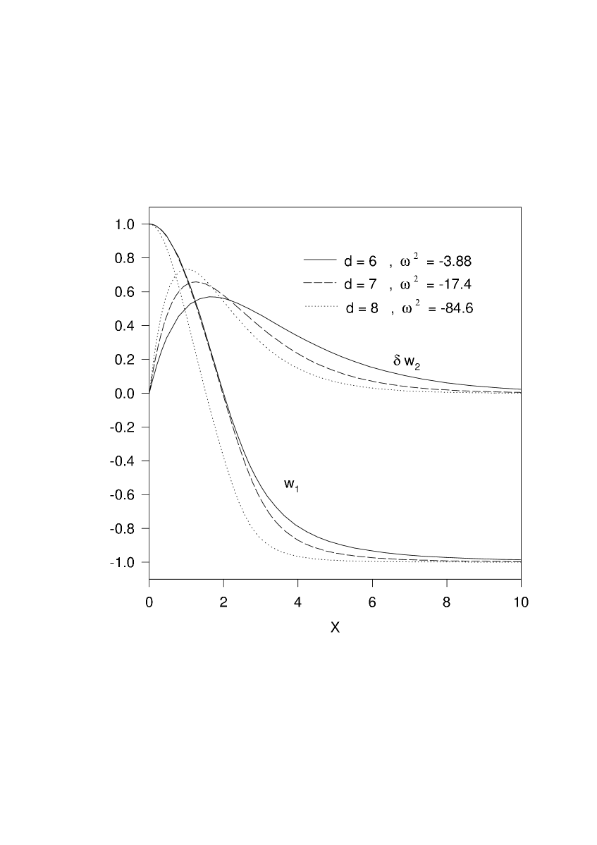
Figure 1: The profiles of the function $w_{1}$ for the sphaleron solutions in $d=6,7,8$, which are practically unchanged when the function $w_{2}$ is perturbed by $\delta w_{2}$. The profiles of the negative modes $\delta w_{2}$ are displayed and the corresponding negative eigenvalues $\omega^{2}$ listed.

In the units choosen, the masses of these solutions are respectively $M(d=6)\approx 4.67$, $M(d=7)\approx 11.3$, $M(d=8)\approx 36.8$. From the numerical profile for $w_{1}$, the different configurations of the path (37)-(39) can be constructed; their energies can further be computed as functions of the parameter $q$. The energy is plotted as a function of the parameter $q$ on Figure 2 for $d=6,7,8$.

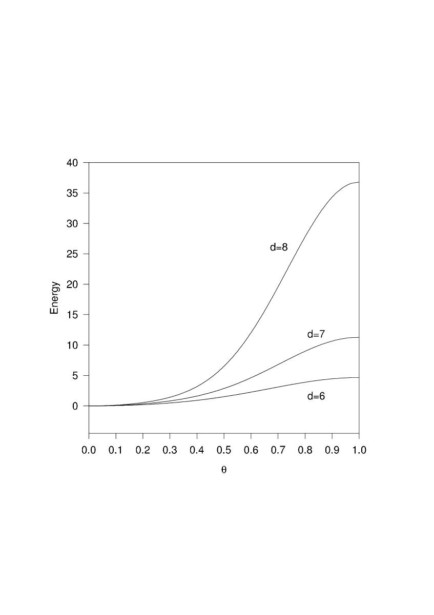
Figure 2: The energy along the path extrapolating between the vacuum and the sphaleron is plotted as a function of $\theta\equiv q/\pi$ for d=6,7,8.

As expected, the figure shows that the configurations on the path have finite energy and that the energy increases monotonically from the vacuum ($q=0$) to the classical solution ($q=\pi$), demonstrating that the classical solution is indeed a sphaleron.

For the cases with even $d$ and nonvanishing CS densities (33)-(34), the energy is plotted also against the CS charges (45)-(46) respectively, on Figure 3.

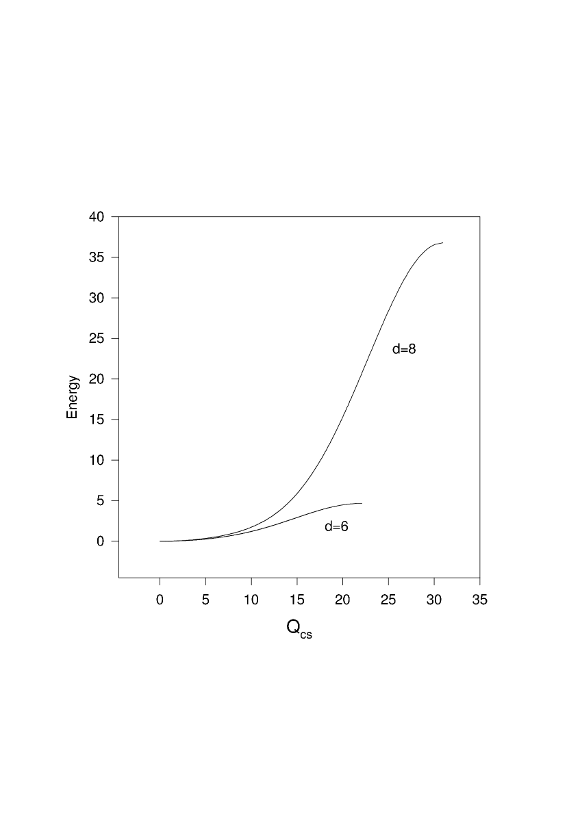
Figure 3: The energy along the path extrapolating between the vacuum and the sphaleron is plotted as a function of $q$ for d=6,8.

4.2 Negative modes

In the second subsection we have carried out an infinitesimal stability analysis by constructing the negative modes and evaluating their negative eigenvalues. We also track, within the limits of validity of this infinitesimal analysis, the growth of the CS charge as a function of the $w_{1}$ and the function $w_{2}$ excited along the direction of instability. For this purpose we consider a perturbation of the classical solution constructed in the previous subsection :

$$\tilde{w}_{1}=w_{1}+\mbox{e}^{i\omega t}\delta w_{1}\quad,\quad\tilde{w}_{2}=w_{2}+\mbox{e}^{i\omega t}\delta w_{2}\quad,\quad\tilde{w}_{3}=0\ ,$$ (47)

choosing again to work in the gauge $w_{3}=0$. Inserting the perturbed solution into the equations of motion and retaining only the linear terms in the fluctuation, we got a system of two decoupled Sturm-Liouville equations in $\delta w_{1}$ and $\delta w_{2}$. The construction of the normal modes is equivalent to finding the normalisable solutions of these equations, which is a problem beyond the scope of this paper. We limit our analysis to the construction of the mode of lowest eigenvalue. The results of [24] strongly suggest that the main mode of instability of our solution should appear in the sector $\delta w_{1}=0$. This turns out to be the case. Technically the negative mode can be constructed by minimising the quadratic form

$$\delta E=2^{(d-2)/2}S_{d-2}\frac{(d-2)}{16}\int drr^{d-4}\left(I_{1}(\delta w_{2}^{\prime})^{2}-I_{2}(\delta w_{2})^{2}\right)$$ (48)

with

$$I_{1}=(\tau_{1}+3\tau_{2}(d-3)(d-4)\frac{1}{r^{4}}(1-w_{1}^{2})^{2})$$ (49)

$$I_{2}=(d-3)\frac{(1-w_{1}^{2})}{r^{2}}\left(\tau_{1}+3\tau_{2}(d-4)\frac{1}{r^{4}}((d-5)(1-w_{1}^{2})^{2}+2r^{2}(w_{1}^{\prime})^{2})\right)\ .$$ (50)

In (49) -(50), the function $w_{1}$ represents the classical sphaleron solution. Inspecting the form of this variational problem we see that it leads to a Sturm-Liouville equation with a potential given by the function $-I_{2}$. This corresponds to a potential well and allowing the existence of a negative mode. We were able to construct numerically one normalised negative mode $\delta w_{2}$ in each case $d=6,7,8$, whose profiles are displayed in Figure 1, together with the profiles of the corresponding classical solution $w_{1}$. The fact that $\delta w_{2}$ presents no node strongly suggests that our solution corresponds to the eigenmode of lowest eigenvalue. These eigenvalues, indeed, appear to be negative and were evaluated to be $-\omega^{2}=3.88,17.4,84.6$ respectively for d=6,7,8, again using the same scale as before.

Finally we evaluate the CS charge $Q_{CS}$ for $d=6$ case, for the configurations of the form $\tilde{w}_{1}=w_{1}$ , $\tilde{w}_{2}=\epsilon\delta w_{2}$, $\epsilon$ being an infinitesimal parameter. We find

$$Q_{CS}(\tilde{w}_{1},\tilde{w}_{2})=Q_{CS}(q=\pi)-1.54\epsilon$$ (51)

where $Q_{CS}(q=\pi)$ is the CS charge of the sphaleron, which for $d=6$ is evaluated from (45), as $Q_{CS}(q=\pi)=22.5$. This shows that the CS charge varies linearly with the parameter $\epsilon$ when the sphaleron is perturbed in the direction of its unstable mode.

5 Summary and Conclusions

We have studied static finite energy solutions to Yang–Mills systems in higher dimensions. The interest in these solutions is that they are gravity decoupling limits of the fully gravitating Einstein–Yang-Mills solutions in higher dimensions. In turn, gravitating YM systems in higher dimensnions are important field theoretic models arising in the study of $Dp$-branes in spacetime dimensions larger than $4$, in the context of the low energy effective action of superstring theory and gauged supergravities. Some of these solutions have sphaleron type instabilities, which must be studied. In this respect the higher dimensional gravitating YM systems are similar to the gravitating YM model in $4$ spacetime dimensions, whose sphaleron like instabilities were studied in detail in [21, 22]. What is different in the higher dimensional cases at hand, versus the $4$ spacetime dimensional case [21, 22], is that unlike for the latter, here we have gravity decoupling limits, and, the sphaleron nature of the gravitating solutions is essentially identical to their flat space counterparts. The sphaleron analysis being appreciably simpler in the flat case, we have chosen to work with those models.

We have restricted our studies to that of spherically symmetric solutions only. This has necessitated certain, rather limited, choices of the gauge groups $G$. These gauge groups turn out to be $SO(d-1)$ and $SO(d)$ in odd spacetime dimensons $d$, and $SO(d)$ only in even $d$. The gauge connections take their values in the spinor reprentations in terms of Dirac matrices, and whenever $G=SO(N)$ is defined for even $N$, we have employed the chiral representations of $SO(N)$. All solutions considered are evaluated numerically and they satisfy the second order Euler–Lagrange equations rather than first order selfduality equations, since the YM systems in question are not scale invariant.

We have shown that in odd spacetime dimensions $d$, the solutions to $SO(d-1)$ YM systems are topologically stable if the representaion of $G$ employed is chiral, i.e. that they are solitons which are stabilised by the Chern–Pontryagin (CP) topological charge. These are the only models which support stable solitons. Should the representations of the $SO(d-1)$ algebra employed not be taken to be the chiral ones, the solutions will be unstable. They are unstable also for the choice of $G=SO(d)$.

In even spacetime dimensions, the solutions turn out to be always unstable, due essentially to the absence of a CP topological charge in the odd spacelike dimensions. For $G=SO(d)$, by employing the chiral representations, we have calculated the Chern–Simons (CS) charges, and have plotted the energy of the noncontractible loops versus the CS charge $Q_{CS}$, highlighting the nature of these solutions as types of sphalerons.

For all the unstable solutions, namely to the $SO(d)$ models in all $d$ dimensional spacetimes, we have constructed the negative modes of the corresponding fluctuation equations and calculated their negative eigenvalues. For the $SO_{\pm}(6)$ solutions in $d=6$ in particular, we have also calculated $Q_{CS}$ perturbatively, showing that in the region of validity the $Q_{CS}$ increases linearly in the pertubation parameter.

We have restricted our study to the simplest model (1), with $p=1$ and $p=2$ terms only, in spacetime dimensions $d=6,7,8$. This limited choice is sufficient to illustrate the questions of stability and instability in the generic cases. The properties demonstrated in the $p=2$ examples studied repeat themselves in every $4p$ dimensions. Thus for example for $p=3$ models, in spacetime dimensions $d=6,8,10,12$ the solutions will be unstable sphalerons, while those in $d=7,9,11$ will be stable, being stabilised by the 3rd, 4th and 5th Pontryagin charges, respectively. If the $d=7$ model chosen in that case does not contain the $p=2$ (in addition to the obligatory $p=3$ term dictated by Derrick)term in the YM hierarchy, then there will be no gravity decoupling limit. In that case the sphaleron analysis must be carried out in the fully gravitating model, following the lines of the analysis in [21, 22] for $d=4$. The same holds true in the case of the $p=2$ model studied here, $d=5$. In that case too there exists no flat space limit so that the sphaleron analysis must again be carried out as in $p=1$, $d=4$ [22, 21]. The latter analysis falls outside the scope of the present work and is deferred to a future study.

Acknowledgements We thank D. Maison for a discussion which gave rise to the present study, and E. Radu for his generous cooperation in the course of this work. This work is supported by Enterprise–Ireland Basic Science Research project SC/2003/390. Y.B. wishes to thank the Belgian FNRS for financial support.

References

- [1] M.B. Green, J.H. Schwarz and E. Witten, Superstring Theory, Cambridge University Press, Cambridge, 1987.
- [2] J. Harvey and A. Strominger, “TASI lectures on quantum aspects of black holes”, hep-th/9209055.
- [3] J. Polchinski, “TASI lectures on D-branes”, hep-th/9611050.
- [4] A.M. Polyakov, Nucl. Phys. B 120 (1977) 459.
- [5] A.A. Tseytlin, Born–Infeld action, suersymmetry and string theory, in Yuri Golfand memorial volume, ed. M. Shifman, World Scientific (2000).
- [6] E. Bergshoeff, M. de Roo and A. Sevrin, Fortsch.Phys. 49 (2001) 433-440; Nucl.Phys.Proc.Suppl. 102 (2001) 50-55.
- [7] M. Cederwall, B. Nilsson and D. Tsimpis, JHEP 0106 (2001) 034.
- [8] R. Bartnik and J. McKinnon, Phys. Rev. Lett. 61 (1988) 141.
- [9] M.S. Volkov and D.V. Gal’tsov, JETP Lett. 50 (1989) 346.
- [10] P. Bizon, Phys. Rev. Lett. 64 (1990) 2844.
- [11] Y. Brihaye, A. Chakrabarti and D.H. Tchrakian, Class. Quant. Grav. 20 (2003) 2765 [hep-th/0202141]
- [12] Yves Brihaye, A. Chakrabarti, Betti Hartmann and D.H. Tchrakian, Phys. Lett. B 561 (2003) 161 [hep-th/0212288]
- [13] see D.H. Tchrakian Yang-Mills hierarchy, Int. J. Mod. Phys. A (Proc.Suppl.) 3A (1993) 584, and references therein.
- [14] P. Breitenlohner, P. Forgacs and D. Maison, Nucl. Phys. B 383 (1992) 357; ibid. 442 (1995) 126.
- [15] K. Lee, V. P. Nair and E. J. Weinberg, Phys. Rev. D 45 (1992) 2751.
- [16] J. Burzlaff and D. H. Tchrakian, J. Phys. A 26 (1993) L1053.
- [17] N.S. Manton, Phys. Rev. D 28 (1983) 2019.
- [18] F.R. Klinkhamer and N.S. Manton, Phys. Rev. D 30 (1984) 2212.
- [19] T. Akiba, H. Kikuchi and T. Yanagida, Phys. Rev. D 38 (1988) 1937.
- [20] E. Witten, Phys. Rev. Lett. 38 (1978) 121.
- [21] D.V. Gal’tsov and M.S. Volkov, Phys. Lett. B 273 (1991) 255.
- [22] M.S. Volkov, Phys. Lett. B 334 (1994) 40.
- [23] F. R. Klinkhamer, Phys. Lett. B 236 (1990) 187.
- [24] Y. Brihaye and J. Kunz, Phys. Lett. B 249 (1990) 90.