Minimal String Theory

Abstract

We summarize recent progress in the understanding of minimal string theory, focusing on the worldsheet description of physical operators and D-branes. We review how a geometric interpretation of minimal string theory emerges naturally from the study of the D-branes. This simple geometric picture ties together many otherwise unrelated features of minimal string theory, and it leads directly to a worldsheet derivation of the dual matrix model.

1 Introduction

Minimal string theories are an important class of tractable, exactly solvable toy models. Despite their simplicity, they are interesting laboratories for the study of string theory, because they contain many of the desirable features of critical string theory, including D-branes, holography and open/closed duality. These general phenomena are realized concretely in minimal string theory through the well-known duality with large $N$ random matrix models. (For reviews and older references, see e.g. [1, 2].) This duality is special and particularly interesting because both dual theories – the pertubative minimal string and the matrix model – are solvable.

Recent progress in the study of Liouville theory [3, 4, 5, 6, 7, 8, 9] has spurred a renewed interest in the minimal string (see e.g. [10, 11, 12, 13, 14, 15, 16, 17, 18, 19]), leading to new insights, some of which we will review here. We will summarize and highlight some new results which are described in much more detail in [15, 18]. We will use worldsheet techniques to derive the dual matrix model. Along the way, a simple geometrical picture will emerge, which will serve to unify many features of the minimal string.

For simplicity, we will focus on bosonic minimal string theories, which are labelled by two relatively prime integers $p<q$. The worldsheet sigma model consists of two parts: $(p,q)$ minimal CFT and Liouville theory. In the next two sections, we will describe these two worldsheet CFTs in detail, and we will show how they are combined to form minimal string theory. Section 2 focuses on the closed minimal string and describes the spectrum of physical operators, while section 3 discusses the D-branes of minimal string theory. The main purpose of these two sections is to collect a diverse list of facts about minimal string theory. These facts are then tied together in section 4, using an auxiliary Riemann surface $\mathcal{M}_{p,q}$ that emerges from the D-branes. In section 5 we show how the same Riemann surface leads to a worldsheet derivation of the matrix model. Finally, various conclusions are collected in section 6.

2 Minimal String Theory on the Worldsheet

2.1 $(p,q)$ minimal CFT

The first ingredient in the worldsheet recipe for minimal string theory is $(p,q)$ minimal CFT (for a review, see e.g. [20]). The minimal models are labelled by their central charge

$$c=1-{6(p-q)^{2}\over pq}<1$$ (1)

Unlike most CFTs, the minimal models have only a finite number of primary operators. We will denote these operators by $\mathcal{O}_{r,s}$ with $r=1,\dots,p-1$, $s=1,\dots,q-1$ and $\mathcal{O}_{p-r,q-s}=\mathcal{O}_{r,s}$. Their conformal dimensions are given by

$$\Delta(\mathcal{O}_{r,s})={(rq-sp)^{2}-(p-q)^{2}\over 4p\,q}$$ (2)

The formula for the dimensions implies that every primary corresponds to a degenerate representation of the Virasoro algebra. That is, they all have null states among their Virasoro descendants. One can systematically exploit this fact to completely constrain the multiplication table of these operators. This results in a set of fusion rules, which take the form

$$[\mathcal{O}_{r_{1},s_{1}}]\times[\mathcal{O}_{r_{2},s_{2}}]=\sum_{r_{3}=1}^{p}\sum_{s_{3}=1}^{q}N_{(r_{1},s_{1})(r_{2},s_{2})(r_{3},s_{3})}[\mathcal{O}_{r_{3},s_{3}}]$$ (3)

where the fusion numbers $N_{(r_{1},s_{1})(r_{2},s_{2})(r_{3},s_{3})}$ are either zero or one. The notation $[\mathcal{O}]$ in (3) is meant to indicate the primary operator $\mathcal{O}$ and all its Virasoro descendants. In other words, the fusion rules tell us how to multiply two Virasoro representations, but they do not tell us the details of the actual operator product coefficients.

2.2 Liouville theory

The other ingredient in the worldsheet construction of minimal string theory is Liouville theory. We can think of this as a theory of a scalar field in two dimensions with action

$$S={1\over 4\pi}\int d^{2}z\,\bigg{(}(\partial\phi)^{2}-4\pi\mu e^{2b\phi}\bigg{)}$$ (4)

The parameter $b>0$ is called the Liouville coupling constant, while $\mu$ is called the cosmological constant. We will assume $\mu\neq 0$ throughout, and we will work in units where $\mu=1$ for simplicity.

For conformal invariance, one also needs to include a “background charge”

$$Q=b+{1\over b}$$ (5)

which results in an asymptotically linear dilaton background at $\phi\to-\infty$. The presence of nonzero $Q$ has several effects. First, it shifts the central charge from the free field value $c=1$ to

$$c=1+6Q^{2}\geq 25$$ (6)

Second, it changes the dimensions of primary operators $V_{\alpha}=e^{2\alpha\phi}$ from $\Delta=-\alpha^{2}$ to

$$\Delta(V_{\alpha})=-\bigg{(}{Q\over 2}-\alpha\bigg{)}^{2}+{Q^{2}\over 4}$$ (7)

Representation theory of the Virasoro algebra with central charge (6) tells us that the primary operators with

$$2\alpha_{r,s}={1\over b}(1-r)+b(1-s),\qquad r,s\in\mathbb{Z}^{+}$$ (8)

correspond to degenerate representations of Virasoro. As in the minimal models, these operators have special fusion rules which lead to a complete solution of Liouville theory [3, 4, 5].

2.3 Minimal string theory

Now we can combine the two ingredients, together with the standard ghosts, to form minimal string theory. We will refer to the minimal CFT as the “matter sector.” Requiring the total central charge of matter plus Liouville to be $c=26$ sets

$$b^{2}={p\over q}$$ (9)

As we will see below, the fact that $b^{2}$ is rational leads to many simplifications in minimal string theory.

Physical operators in minimal string theory are built out of the operators of the Liouville, matter, and ghost sectors. As usual, BRST invariance requires physical operators to have dimension zero. However, in contrast with critical string theory, in minimal string theory there are BRST invariant physical operators at all ghost numbers [21]. This is a direct consequence of the existence of degenerate operators in Liouville theory and the matter sector. The most important operators for our purposes are those at ghost number zero and one. Let us now describe them in detail, starting with the operators at ghost number zero.

Clearly, by ghost number conservation, the ghost number zero operators form a ring under multiplication by the OPE [22]. This ring is called the ground ring, and its elements take the form

$$\begin{split}&\hat{\mathcal{O}}_{r,s}=\mathcal{L}_{r,s}\cdot\mathcal{O}_{r,s}e^{2\,\alpha_{r,s}\,\phi},\qquad 1\leq r\leq p-1\ ,\quad 1\leq s\leq q-1\end{split}$$ (10)

with $\alpha_{r,s}$ given by (8) and $\mathcal{L}_{r,s}$ a certain polynomial in ghosts and Virasoro generators. Note that the range of $r$ and $s$ means that there are exactly twice as many ground ring elements as primaries in the minimal model.

The multiplication of the ring elements is constrained by the fusion rules in the matter and Liouville CFTs. This allows us to completely determine the ring relations, up to a few coefficients which are justified later. In terms of the ring generators

$$\begin{split}&X\equiv{1\over 2}\hat{\mathcal{O}}_{2,1},\qquad Y\equiv{1\over 2}\hat{\mathcal{O}}_{1,2}\end{split}$$ (11)

(note that $\hat{\mathcal{O}}_{1,1}=1$) we find that

$$\hat{\mathcal{O}}_{r,s}=U_{s-1}(X)U_{r-1}(Y)$$ (12)

where the $U_{s-1}(X)$ are Chebyshev polynomials of the second kind,

$$U_{s-1}(X=\cos\theta)={\sin s\,\theta\over\sin\theta}$$ (13)

Since these polynomials are also the $SU(2)$ characters, their products are the $SU(2)$ fusion rules. In particular, the coefficients in this multiplication table are either zero or one.

The formula (12) for the ring elements would obviously be incorrect if it were not supplemented by additional relations in the ring, since otherwise we would find infinitely many ring elements. Comparing with the range of $r$ and $s$ in (10), we see that the correct ring relations to impose are

$$U_{q-1}(X)=U_{p-1}(Y)=0$$ (14)

(With only $X$ present, this is familiar from the representation ring of $\widehat{SU(2)}$.) The ring relations (14) preserve the simplicity of the multiplication table, i.e. all the coefficients are still just zero or one! In the traditional worldsheet analysis of the minimal string, this simple answer would arise as a surprising cancellation between complicated OPEs of operators in the minimal CFT and Liouville theory.

Having understood the ground ring and its structure in some detail, we can now apply our knowledge to the study of the operators at other ghost numbers. Ghost number conservation implies that the set of all operators at a given ghost number form a module under the action of the ground ring. The simplest such module consists of the ghost number one “tachyon” operators:

$$\mathcal{T}_{r,s}=c\,\bar{c}\,\mathcal{O}_{r,s}e^{2\beta_{r,s}\phi},\quad 1\leq r\leq p-1\ ,\quad 1\leq s\leq q-1$$ (15)

BRST invariance requires $\Delta(\mathcal{T}_{r,s})=0$, which according to (2) and (7) is satisfied when

$$\begin{split}&2\beta_{r,s}={p+q-|rq-sp|\over\sqrt{p\,q}}\cr\end{split}$$ (16)

Unlike the ground ring elements (but like the minimal model primaries), the tachyons satisfy a reflection relation:

$$\mathcal{T}_{p-r,q-s}=\mathcal{T}_{r,s}$$ (17)

Thus there are exactly as many independent tachyons as primaries in the minimal model.

Since the tachyons form a module under the action of the ground ring, a trivial application of the fusion rules in the matter CFT leads to the following simple formula for the tachyons in terms of the ring elements:

$$\mathcal{T}_{r,s}=\hat{\mathcal{O}}_{r,s}\mathcal{T}_{1,1}=U_{s-1}(X)U_{r-1}(Y)\mathcal{T}_{1,1}$$ (18)

This formula is actually quite useful. We mention two applications:

• The tachyons obviously do not form a faithful representation of the ring, since there are half as many tachyons as ground ring elements. Indeed, combining the reflection relation (17) with (18), we obtain a new relation in the module:

  $$T_{p}(Y)-T_{q}(X)=0$$ (19)

  with $T_{p}(Y)$ the Chebyshev polynomials of the first kind,

  $$T_{p}(Y=\cos\theta)=\cos p\,\theta$$ (20)

  The relation (19) can also be written as $U_{p-2}(Y)-U_{q-2}(X)=0$. This relation as well as (14) were first discovered as relations in the fusion ring in [24].

• Using the ring and its module, we can easily derive some correlation functions. For instance,

  $$\begin{split}\langle\mathcal{T}_{r_{1},s_{1}}\mathcal{T}_{r_{2},s_{2}}\mathcal{T}_{r_{3},s_{3}}\rangle&=\langle\hat{\mathcal{O}}_{r_{1},s_{1}}\hat{\mathcal{O}}_{r_{2},s_{2}}\hat{\mathcal{O}}_{r_{3},s_{3}}\mathcal{T}_{1,1}\mathcal{T}_{1,1}\mathcal{T}_{1,1}\rangle\cr&=N_{(r_{1},s_{1})(r_{2},s_{2})(r_{3},s_{3})}\end{split}$$ (21)

  In other words, the three-point functions of tachyon operators in $(p,q)$ minimal string theory are precisely the fusion rules of the associated $(p,q)$ minimal CFT. This surprisingly simple result had been derived previously using much more complicated methods in [25, 26, 27]. Our new derivation shows why the correlators are so simple: it is due to the underlying simplicity of the ground ring.

3 D-branes in Minimal String Theory

In the previous section, we described how minimal string theories are put together at the worldsheet level, focusing on the closed string sector. Now let us turn to the open strings and describe how to construct the D-branes of minimal string theory. These are built out of the D-branes of Liouville theory and minimal CFT. They are conveniently described using the boundary state formalism, which associates to every D-brane a “Cardy state” labelled by a highest-weight Virasoro representation in the open string channel.

In the minimal models, the Cardy states are in one-to-one correspondence with the Virasoro representations, and therefore a given minimal model has a finite number of branes given by the number of primary operators. The branes are usually denoted by $|k,l\rangle$, with $k$ and $l$ taking the same integer values as for the primaries $\mathcal{O}_{k,l}$ of the minimal model.

The D-branes of Liouville theory were discovered more recently through the work of [6, 7, 8]. There are two kinds of D-branes in Liouville theory. The first kind, called FZZT branes [6, 7], fall into a continuous family parametrized by the “boundary cosmological constant” $\mu_{B}$ which multiplies the boundary interaction

$$\delta\,S=\mu_{B}\oint e^{b\,\phi}$$ (22)

Solving the equation of motion for $\phi$ on a worldsheet with bulk action (4) and boundary interaction (22) gives rise to Neumann-like boundary conditions for the Liouville field:

$$\partial_{\sigma}\phi=-2\pi b\mu_{B}e^{b\phi}$$ (23)

The FZZT branes are extended semi-infinitely in $\phi$ space. One way to see this is using the minisuperspace wavefunction of the FZZT brane. In the semiclassical $b\to 0$ limit, this is given by

$$\psi(\phi)=\langle\phi|\mu_{B}\rangle=e^{-\mu_{B}\,e^{b\,\phi}}$$ (24)

According to (24), the FZZT brane comes in from $\phi=-\infty$ and dissolves at $\phi\approx-{1\over b}\log\mu_{B}$ (see figure 1).

In the boundary state formalism, the FZZT brane labelled by $\mu_{B}$ corresponds to a Cardy state $|\,\sigma\rangle$ labelled by the nondegenerate Virasoro representation with dimension

$$\Delta={1\over 4}\sigma^{2}+{Q^{2}\over 4}$$ (25)

(in the notation of (7), this corresponds to $\alpha={Q\over 2}+{i\sigma\over 2}$) where $\sigma$ and $\mu_{B}$ are related by

$$\mu_{B}=\cosh\pi\,b\,\sigma$$ (26)

This expression allows us to analytically continue $\sigma\in\mathbb{C}$, which is a infinite multiple cover of $\mu_{B}\in\mathbb{C}$.

The second kind of Liouville branes are the ZZ branes [8]. These fall into a discrete, two-parameter family parametrized by integers $m,n\geq 1$, and they are all localized in the strong coupling region $\phi\to+\infty$. In the boundary state formalism, the ZZ branes correspond to the degenerate representations of Liouville theory, which according to (8) and the map $\alpha={Q\over 2}+{i\sigma\over 2}$ are given by

$$\sigma=\sigma(m,n)=i\bigg{(}{m\over b}+nb\bigg{)},\qquad m,n\in\mathbb{Z}^{+}$$ (27)

Subtracting the null vectors in the degenerate representation leads to a formula for the boundary state of the ZZ branes in terms of the FZZT branes [8]

$$|m,n\rangle=|\,\sigma(m,n)\rangle-|\,\sigma(m,-n)\rangle$$ (28)

Notice that the two FZZT branes in (28) have the same value of the boundary cosmological constant [11]:

$$\mu_{B}=(-1)^{m}\cos\pi\,n\,b^{2}$$ (29)

We will give a geometric interpretation to this fact below.

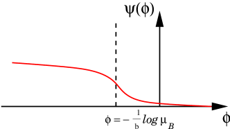
Figure 1: A plot of the minisuperspace wavefunction of the FZZT brane. The dotted line denotes the location of the “tip” of the FZZT brane in $\phi$ space.

Having described the branes of Liouville theory and minimal CFT, we are now ready to form the D-branes of minimal string theory. We simply tensor together a boundary state from Liouville theory (either FZZT or ZZ) together with a boundary state $|k,l\rangle$ from the minimal model. (Note that we also have to set $b=\sqrt{p\over q}$ in the formulas above.) However, not all of these tensored boundary states are linearly independent. Before we can write down the actual list of D-branes in minimal string theory, there are three subtleties we have to take into account.

• Naively, it would seem that there are a number of different FZZT branes and ZZ branes, distinguished by the choice of matter state. However, it turns out that only the branes with matter state $|1,1\rangle$ are independent. The FZZT branes with matter state $|k,l\rangle$ are related to those with matter state $|1,1\rangle$ by the identifications

  $$\begin{split}|\,\sigma&;k,l\rangle=\sum_{m^{\prime}=-(k-1),2}^{k-1}\ \sum_{n^{\prime}=-(l-1),2}^{l-1}|\,\sigma+{i(m^{\prime}q+n^{\prime}p)\over\sqrt{pq}};1,1\rangle\cr\end{split}$$ (30)

  The ZZ branes satisfy the same relations, thanks to (28). Note that these identifications are meant to be statements about the BRST cohomology, i.e. the branes on the two sides of (30) cannot be distinguished by any physical observables.

• Another consequence of the BRST cohomology is that not all of the FZZT branes labelled by $\sigma$ are distinct. It turns out that the independent FZZT branes are reduced to $|\,\sigma\rangle\to|\,z\rangle$ with the parameter $z$ defined to be

  $$z=\cosh{\pi\sigma\over\sqrt{pq}}$$ (31)

  In the next section we will see that $z$ plays a central role in the geometrical interpretation of minimal string theory.

• Finally, there are subtleties having to do with Virasoro representation theory for rational $b^{2}$. Without getting into the details, let us just say that taking them into account (and imposing the BRST cohomology) reduces the infinite family of Liouville ZZ branes to a finite number $|m,n\rangle$ with $1\leq m\leq p-1$, $1\leq n\leq q-1$, and $qm-pn>0$ [15].

Combining these three facts, we arrive at the final list of independent D-branes in minimal string theory:

$$\begin{split}{\rm FZZT}:\quad&|\,z\rangle\otimes|1,1\rangle,\qquad\quad\,\,\,z\in\mathbb{C}\cr{\rm ZZ}:\quad&|\,m,n\rangle\otimes|1,1\rangle,\qquad 1\leq m\leq p-1,\quad 1\leq n\leq q-1,\quad qm-pn>0\end{split}$$ (32)

4 Geometric Interpretation

In the previous two sections, we collected many different facts about open and closed minimal string theory. Now let us show how these seemingly unrelated facts combine to form a simple geometric picture of minimal string theory. The starting point is the observation that the disk amplitude $Z(\mu_{B})$ of the FZZT brane is not a single valued function of $\mu_{B}$. Instead, if we define

$$x\equiv\mu_{B}=\cosh{\pi b\sigma},\qquad y\equiv\partial_{\mu_{B}}Z(\mu_{B})=\cosh{\pi\sigma\over b}$$ (33)

then $x$ and $y$ satisfy the algebraic equation

$$F_{p,q}(x,y)=T_{p}(y)-T_{q}(x)=0$$ (34)

This describes a genus ${(p-1)(q-1)\over 2}$ Riemann surface $\mathcal{M}_{p,q}$ with ${(p-1)(q-1)\over 2}$ pinched $A$-cycles (singularities). An example of such a surface is shown in figure 2. The singularities occur at the simultaneous solution of (34) and

$$\begin{split}&T_{p}^{\prime}(y)=p\,U_{p-1}(y)=0\cr&T_{q}^{\prime}(x)=q\,U_{q-1}(x)=0\end{split}$$ (35)

We recognize (34) and (35) to be precisely the ground ring relations and the relation in the tachyon module! Thus the algebraic structure of the ground ring is directly related to the geometric structure of the FZZT brane.

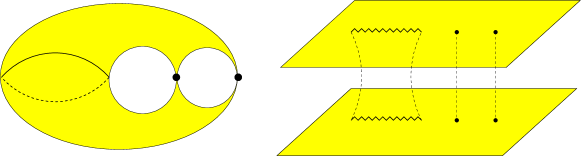
Figure 2: An example of a Riemann surface with pinched cycles, viewed also as a double-cover of the complex plane.

As promised, the parameter $z$ defined in (31) plays an important role in the geometrical description: it is the uniformizing parameter of $\mathcal{M}_{p,q}$. By this we mean the following. It is trivial to see that the equation (34) for the surface is solved by

$$x=T_{p}(z),\qquad y=T_{q}(z)$$ (36)

This means that, apart from the singularities, every point $(x,y)$ on the surface is in one-to-one correspondence with a point $z$ in the complex plane. Thus, the complicated structure of $\mathcal{M}_{p,q}$ is mapped to the complex $z$ plane by (36), i.e. the surface is uniformized by (36). The singularities are then points where this one-to-one correspondence breaks down. For the surfaces described by (34), there are exactly two values of $z$ corresponding to a given singularity.

Since the surface $\mathcal{M}_{p,q}$ arose from the FZZT disk amplitude, it is not surprising that it encodes the FZZT branes in a natural way. What is surprising, however, is that it also knows about the ZZ branes. Let us see how this comes about. Consider the following one form on $\mathcal{M}_{p,q}$:

$$\omega\equiv y\,dx$$ (37)

Then the D-branes correspond to line integrals of $\omega$. The FZZT brane is obviously an integral of $\omega$ along an open contour:

$$Z(x)=\int_{P}^{x}\omega$$ (38)

On the other hand, the $(m,n)$ ZZ brane is a difference between two FZZT branes with the same value of $x=x_{m,n}=(-1)^{m}\cos{\pi p\,n\over q}$, so it corresponds to an integral of $\omega$ along a closed contour:

$$Z(m,n)=\oint_{B_{m,n}}\omega$$ (39)

This gives a geometric interpretation to the relation (28) between the ZZ and FZZT boundary states.

Note that since the disk amplitude $Z(m,n)$ is nonzero, the contour of the $(m,n)$ brane must be a nontrivial cycle of the surface. We can confirm this geometrically by noticing that $B_{m,n}$ passes through $(x_{m,n},y_{m,n})$, which according to (35) is a singularity of the surface. Therefore $B_{m,n}$ is the conjugate $B$-cycle to the pinched $A$-cycle located at $(x_{m,n},y_{m,n})$. These contours are shown in figure 3.

We can also rephrase the preceding paragraph in a way that leads to a new insight about the ZZ branes. The association of the ZZ branes with the singularities of the surface means that there is a sense in which they are “located” at the singularities. We can make this more precise by recalling that the equations for the singularities are the same as the ground ring relations. This suggests that the ZZ branes and the ground ring are related in some natural way. Indeed, one can show that the ZZ branes are eigenstates of the ground ring elements, with eigenvalues $(x_{m,n},y_{m,n})$:

$$\begin{split}X|m,n\rangle&=x_{m,n}|m,n\rangle\cr Y|m,n\rangle&=y_{m,n}|m,n\rangle\end{split}$$ (40)

We note in passing that this leads to a simple derivation of the ring relations (12) and (14). More to the point, however, (40) makes precise the idea that the ZZ branes are located at the singularities. According to (40), we can think of the ring generators $X$ and $Y$ as measuring the “position” of the ZZ brane on $\mathcal{M}_{p,q}$.

So far we have been considering a special closed-string background corresponding to the Liouville action (4) with the cosmological constant interaction. This gives rise to the surface described by (34). We can also consider more general backgrounds, obtained by adding other physical operators to the worldsheet action (e.g. the tachyons (15)). These will deform the equation of the Riemann surface, but in such a way as to preserve its geometrical properties. In particular, the surface will still be a finite-sheeted cover of the complex $x$ plane, and it will still have a number of singularities. Thus the deformed surface will still possess a uniformizing parameter $z$. In fact, one can characterize the deformations as deformations of the uniformizing map (36):

$$\delta x=\epsilon R(z),\qquad\delta y=\epsilon S(z)$$ (41)

with $R$ and $S$ polynomials in $z$. One can show that infinitesimal deformations by closed string states correspond to singularity preserving deformations of $\mathcal{M}_{p,q}$ of the form (41). Conversely, the list of all polynomial deformations to $x(z)$ and $y(z)$ captures the spectrum of physical closed string states at all ghost numbers.

Of course, we can also imagine deformations of the surface which do not preserve the singularities. These correspond to adding $\mathcal{O}\left({1/g_{s}}\right)$ background ZZ branes. This has a nice geometrical realization in terms of the contours of the surface: the period $\oint_{B_{m,n}}\omega$ creates $(m,n)$ ZZ branes, while the conjugate period $\oint_{A_{m,n}}\omega$ measures how many are present:

$$\oint_{A_{m,n}}\omega=g_{s}N_{m,n}$$ (42)

In target space, these deformations can be thought of as adding background tachyons with the “wrong” Liouville dressing $\alpha\geq{Q\over 2}$. Such tachyons diverge in the strong coupling region $\phi\to+\infty$, and so they are naturally identified with the addition of background ZZ branes [18].

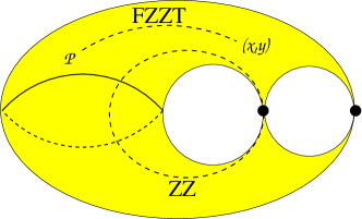
Figure 3: A Riemann surface with examples of FZZT and ZZ contours.

5 Deriving the Dual Matrix Model

Besides providing a unified description of minimal string theory, the geometric picture outlined in the previous section has an important added benefit: it leads directly to the dual matrix model. The fact that minimal strings are dual to certain large $N$ random matrix models is well known (for a review and references, see [1, 2]), and the duality has been verified in many different ways. Now, with our improved knowledge of the worldsheet description of minimal string theory, we can shed new light on this duality and basically derive it.

For simplicity, let us focus on the models with $(p=2,q=2k-1)$, which are dual to the one matrix model

$$Z(g)=\int dM\,e^{-{1\over g}\rm Tr\,V(M)}$$ (43)

with $M$ an $N\times N$ Hermitian matrix. The surface for $p=2$ is

$$2y^{2}-1=T_{2k-1}(x)$$ (44)

This describes a double cover of the complex $x$ plane on which $y(x)$ is single valued. The two sheets are connected along a cut $-\infty<x\leq-1$. There are also $k$ singularities (pinched cycles) located at

$$\bigg{(}x_{n}=\cos{2\pi n\over 2k-1}\ ,\ y_{n}=0\bigg{)}\ ,\quad n=1,...,k$$ (45)

Now we can proceed to match the surface with quantities in the matrix model. The discontinuity of $y(x)$ along the cut is the eigenvalue density:

$$\rho(x)={\rm Im}\sqrt{2+2\,T_{2k-1}(x)}$$ (46)

More generally, $y(x)$ corresponds to the force on an eigenvalue (note that $y=0$ at the singularities), and the disk amplitude of the FZZT brane

$$Z(x)=\int^{x}y\,dx^{\prime}=-{1\over 2}V_{eff}(x)$$ (47)

is the effective potential of a probe eigenvalue. Since the ZZ branes are located at the singularities, we conclude that they correspond to eigenvalues at the stationary points of $V_{eff}(x)$ (where $y=0$). The cut at $x<-1$ corresponds to the Fermi sea – the ZZ branes decay (condense) and fill the Fermi sea. The matrix $M$ of the matrix model then corresponds to open strings between $N\to\infty$ condensed ZZ branes.

The FZZT brane in the matrix model is described by the macroscopic loop operator

$$W(x)={\rm Tr}\,{\rm log}(x-M)$$ (48)

Thus $Z(x)=\langle W(x)\rangle$, and $y=\partial_{x}Z(x)$ is the resolvent of the matrix model. The full, nonperturbative FZZT brane corresponds to worldsheets with any number of boundaries (and handles). This is accomplished in the matrix model by exponentiating $W(x)$, leading to a simple formula for the FZZT-brane creation operator

$$\Psi(x)\sim\det(x-M)$$ (49)

Note that we can write this as a Grassmann integral over $2N$ fermions $\chi_{i}$ and $\chi^{\dagger}_{i}$:

$$\det(x-M)=\int d\chi^{\dagger}d\chi\,e^{\chi^{\dagger}(x-M)\chi}$$ (50)

We interpret $\chi$, $\chi^{\dagger}$ to be fermionic open strings between ZZ and FZZT branes.

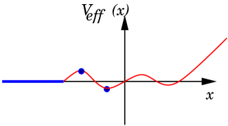
Figure 4: An example of the effective potential of the matrix model. The blue line denotes the branch cut in the effective potential (corresponding to the Fermi sea), and the blue dots at the local extrema denote stationary eigenvalues corresponding to ZZ branes.

6 Conclusions

We have seen how an effective “target space,” consisting of a certain Riemann surface $\mathcal{M}_{p,q}$, emerges as the moduli space of branes. This surface captures many of the properties of the minimal string, including its D-branes, its spectrum of closed-string operators, and their correlation functions. The D-branes correspond to integrals of a certain one-form $\omega$ on the Riemann surface, while the deformations of the surface encode the closed-string observables (singularity preserving) and the spectrum of localized branes (singularity destroying).

We also saw how this geometric picture is complemented by the algebraic structure of the ground ring. In particular, the ring relations controlled the correlation functions, the defining equation of the surface, and the location of its singularities.

Finally, we gave a worldsheet derivation of the matrix model, and added a new perspective to the understanding that the eigenvalues of the matrix model are associated with D-branes [28, 29, 10, 12].

Let us conclude with the following comment on the regime of validity of our results. Clearly, the geometrical picture described here (which emerged from the disk amplitude of the FZZT brane) is only meant to apply at the level of perturbation theory in the string coupling. In fact, nonperturbative effects change the “target space” $\mathcal{M}_{p,q}$ very dramatically [30]. Order-by-order in perturbation theory, the moduli space of FZZT branes is a multiple cover of the complex $x$ plane. But the exact FZZT observables are entire functions of $x$, and therefore the exact moduli space is reduced to just a single copy of the $x$ plane [30].

References

- [1] P. H. Ginsparg and G. W. Moore, “Lectures on 2-D gravity and 2-D string theory,” arXiv:hep-th/9304011.
- [2] P. Di Francesco, P. H. Ginsparg and J. Zinn-Justin, “2-D Gravity and random matrices,” Phys. Rept. 254, 1 (1995) [arXiv:hep-th/9306153].
- [3] H. Dorn and H. J. Otto, “Some conclusions for noncritical string theory drawn from two and three point functions in the Liouville sector,” arXiv:hep-th/9501019.
- [4] J. Teschner, “On the Liouville three point function,” Phys. Lett. B 363, 65 (1995) [arXiv:hep-th/9507109].
- [5] A. B. Zamolodchikov and A. B. Zamolodchikov, “Structure constants and conformal bootstrap in Liouville field theory,” Nucl. Phys. B 477, 577 (1996) [arXiv:hep-th/9506136].
- [6] V. Fateev, A. B. Zamolodchikov and A. B. Zamolodchikov, “Boundary Liouville field theory. I: Boundary state and boundary two-point function,” arXiv:hep-th/0001012.
- [7] J. Teschner, “Remarks on Liouville theory with boundary,” arXiv:hep-th/0009138.
- [8] A. B. Zamolodchikov and A. B. Zamolodchikov, “Liouville field theory on a pseudosphere,” arXiv:hep-th/0101152.
- [9] B. Ponsot and J. Teschner, “Boundary Liouville field theory: Boundary three point function,” Nucl. Phys. B 622, 309 (2002) [arXiv:hep-th/0110244].
- [10] J. McGreevy and H. Verlinde, “Strings from tachyons: The c = 1 matrix reloaded,” JHEP 0312, 054 (2003) [arXiv:hep-th/0304224].
- [11] E. J. Martinec, “The annular report on non-critical string theory,” arXiv:hep-th/0305148.
- [12] I. R. Klebanov, J. Maldacena and N. Seiberg, “D-brane decay in two-dimensional string theory,” JHEP 0307, 045 (2003) [arXiv:hep-th/0305159].
- [13] J. McGreevy, J. Teschner and H. Verlinde, “Classical and quantum D-branes in 2D string theory,” JHEP 0401, 039 (2004) [arXiv:hep-th/0305194].
- [14] I. R. Klebanov, J. Maldacena and N. Seiberg, “Unitary and complex matrix models as 1-d type 0 strings,” arXiv:hep-th/0309168.
- [15] N. Seiberg and D. Shih, “Branes, rings and matrix models in minimal (super)string theory,” JHEP 0402, 021 (2004) [arXiv:hep-th/0312170].
- [16] D. Gaiotto and L. Rastelli, “A paradigm of open/closed duality: Liouville D-branes and the Kontsevich model,” arXiv:hep-th/0312196.
- [17] M. Hanada, M. Hayakawa, N. Ishibashi, H. Kawai, T. Kuroki, Y. Matsuo and T. Tada, “Loops versus matrices: The nonperturbative aspects of noncritical string,” Prog. Theor. Phys. 112, 131 (2004) [arXiv:hep-th/0405076].
- [18] D. Kutasov, K. Okuyama, J. w. Park, N. Seiberg and D. Shih, “Annulus amplitudes and ZZ branes in minimal string theory,” JHEP 0408, 026 (2004) [arXiv:hep-th/0406030].
- [19] J. Ambjorn, S. Arianos, J. A. Gesser and S. Kawamoto, “The geometry of ZZ-branes,” arXiv:hep-th/0406108.
- [20] P. Di Francesco, P. Mathieu and D. Senechal, “Conformal field theory,”
- [21] B. H. Lian and G. J. Zuckerman, “New selection rules and physical states in 2-D gravity: Conformal gauge,” Phys. Lett. B 254, 417 (1991).
- [22] E. Witten, “Ground ring of two-dimensional string theory,” Nucl. Phys. B 373, 187 (1992) [arXiv:hep-th/9108004].
- [23] N. Seiberg, “Notes On Quantum Liouville Theory And Quantum Gravity,” Prog. Theor. Phys. Suppl. 102, 319 (1990).
- [24] P. Di Francesco and J. B. Zuber, “Fusion potentials. 1,” J. Phys. A 26, 1441 (1993) [arXiv:hep-th/9211138].
- [25] P. Di Francesco and D. Kutasov, “Unitary Minimal Models Coupled To 2-D Quantum Gravity,” Nucl. Phys. B 342, 589 (1990).
- [26] M. Goulian and M. Li, “Correlation Functions In Liouville Theory,” Phys. Rev. Lett. 66, 2051 (1991).
- [27] P. Di Francesco and D. Kutasov, “World sheet and space-time physics in two-dimensional (Super)string theory,” Nucl. Phys. B 375, 119 (1992) [arXiv:hep-th/9109005].
- [28] S. H. Shenker, “The Strength Of Nonperturbative Effects In String Theory,” RU-90-47 Presented at the Cargese Workshop on Random Surfaces, Quantum Gravity and Strings, Cargese, France, May 28 - Jun 1, 1990
- [29] J. Polchinski, “Combinatorics of boundaries in string theory,” Phys. Rev. D 50, 6041 (1994) [arXiv:hep-th/9407031].
- [30] J. Maldacena, G. W. Moore, N. Seiberg and D. Shih, “Exact vs. semiclassical target space of the minimal string,” arXiv:hep-th/0408039.