Stabilizing Moduli with String Cosmology

Abstract

In this talk I will discuss the role of finite temperature quantum corrections in string cosmology and show that they can lead to a stabilization mechanism for the volume moduli. I will show that from the higher dimensional perspective this results from the effect of states of enhanced symmetry on the one-loop free energy. These states lead not only to stabilization, but also suggest an alternative model for $\Lambda$CDM. At late times, when the low energy effective field theory gives the appropriate description of the dynamics, the moduli will begin to slow-roll and stabilization will generically fail. However, stabilization can be recovered by considering cosmological particle production near the points of enhanced symmetry leading to the process known as moduli trapping.

1 String Gases in $10D$

1.1 Initial Conditions

One problem in string cosmology is the issue of initial conditions. Not only must models of string cosmology address the standard initial condition problems in cosmology, but string theory also predicts the existence of extra dimensions. The usual prescription for dealing with the extra dimensions is to take them small, stable, and unobservable. However a complete model of string cosmology should explain how this came about and why the explicit breaking of Lorentz invariance should be allowed. A step in this direction was first proposed by Brandenberger and Vafa[1]. They argued that, by considering the dynamics of a string gas in nine, compact spatial dimensions initially taken at the string scale, one could explain why three dimensions grow large while six stay compact. The crux of their argument is based on the fact that in addition to the usual Kaluza Klein modes of a particle on a compact space, strings also possess winding modes. These extra degrees of freedom will generically halt cosmological expansion; however, if these modes could annihilate with their anti-partners this would allow the dimension they occupy to expand. Then, the fact that strings generically intersect (interact) in at most three spatial dimensions means that in the remaining six dimensions thermal equilibrium cannot be maintained. Thus, the winding modes will drop out of equilibrium and the six spatial dimensions will be frozen near the string scale. Furthermore, once all the winding modes in the three large dimensions annihilate, the universe emerges filled with a gas of momentum modes, which evolves as a radiation dominated universe.

1.2 String Gases at Finite Temperature

The usual starting point of string cosmology is the action,

$$S=\frac{1}{2\kappa^{2}}\int d^{d+1}x\sqrt{-g}e^{-2\varphi}\Biggl{(}R+4(\nabla\varphi)^{2}-\frac{1}{12}H^{2}+{\mathcal{O}}(\alpha^{\prime})\Biggr{)}+{\mathcal{O}}(g_{s}).$$ (1)

For simplicity we will ignore the Ramond sector and set $H=0$. Here we have in mind the heterotic string on a toroidal background. Motivated by the Brandenberger-Vafa scenario we will take the background to be $\mathbb{R}^{4}\times T^{6}$, where we assume that the three spatial dimensions have grown large enough to be approximated by an FRW universe and the six small dimensions are toroidal and near the string scale. To include time dependence we make use of the adiabatic approximation, which implies that we can replace static quantities by slow varying functions of time.

The action (1) represents a double expansion in both the string coupling $g_{s}\sim e^{\langle\varphi\rangle}$ and the string tension, $T=\frac{1}{4\pi\alpha^{\prime}}$. We now want to include terms coming from $g_{s}$ corrections at finite temperature[2, 3]. Let us consider the $1$-loop free energy

$$F=TZ_{1}\sim\beta^{-1}\sum e^{-\beta M(n,\omega,N,\bar{N})},$$ (2)

where $Z_{1}$ is the one loop partition function, $M(n,\omega,N,\bar{N})$ is the string mass, and $\beta=1/T$ is the inverse temperature. In the early universe we are interested in temperatures near or below the string scale ($\beta\gtrsim\sqrt{\alpha^{\prime}}$) where the major contribution to the one-loop free energy can be seen to come from the massless modes of the string.

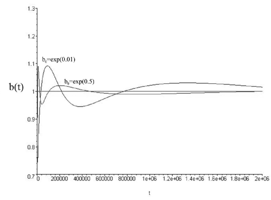
Figure 1: The evolution of the volume modulus of the extra dimensions for different initial values near the self-dual radius. We see that the moduli are eventually stabilized at the self-dual radius where the pressure is found to vanish.

In the case of the heterotic string there are additional massless states that occur at the special radius $R=\sqrt{\alpha^{\prime}}$. These extra states include winding and momentum modes of the string. To understand the dynamics that result by including these states we can find the energy density and pressure, which follow from the free energy as

$$\rho=\frac{1}{V}\frac{\partial}{\partial\beta}(\beta F)$$

$$p_{i}=-\frac{1}{9V}\frac{\partial F}{\partial(lnR_{i})},$$ (3)

where $V$ is the spatial volume and $R_{i}$ is the scale factor in the $ith$ direction. As discussed above, we take initial conditions where three dimensions have grown large and six remain near the string scale. For such initial data, the above pressure in three dimensions corresponds to the equation of state of a radiation dominated universe $p_{3}=\frac{1}{3}\rho$, whereas the pressure in the small dimensions gives the behavior,

$$p_{6}<0\;\;\text{for}\;\;R_{6}>\sqrt{\alpha^{\prime}}\;\;\;\;\text{and}\;\;\;\;p_{6}>0\;\;\text{for}\;\;R_{6}<\sqrt{\alpha^{\prime}}.$$ (4)

In dilaton gravity negative pressure implies a contracting universe, whereas positive pressure leads to expansion. Thus, as can be seen in Figure 1, pressure leads to a stabilizing effect for the scale factor of the extra dimensions driving the radius toward the enhanced symmetry point $R_{(6)}=\sqrt{\alpha^{\prime}}$ where the pressure vanishes. At this location the gauge symmetry of the heterotic string is enhanced, $E_{8}\times E_{8}+U(1)^{6}\longrightarrow E_{8}\times E_{8}+SU(2)^{6}$.

In addition to stabilizing the volume moduli, it has been shown that the remnant string modes, if taken in the dark sector, can also lead to an interesting cold dark matter candidate[4, 5] (see also[6]).

2 Moduli Trapping and Stabilization in $4D$

If one attempts to extend the arguments above to the $4D$ effective field theory, one finds that the stabilization mechanism no longer holds. This is not surprising since the pressure in the extra dimensions has no analog from the $4D$ perspective. However, one thing that should remain is the idea of enhanced symmetry.

Recall that it was the contribution of the enhanced symmetry states near $R=\sqrt{\alpha^{\prime}}$ that led to the pressure terms in (4) stabilizing the extra dimensions. We can account for these enhanced states from the effective field theory (EFT) perspective by considering the effects of particle production near the enhanced symmetry point, $R=\sqrt{\alpha^{\prime}}$.

To understand how this mechanism works let us consider the simplest case of heterotic strings on the background $\mathbb{R}^{4}\times S^{1}$. The low energy effective action comes from the compactification of the action (1). The dynamics are then given by dilaton gravity coupled to a chiral $U(1)$ gauge theory,

$${\mathcal{L}}_{\text{m}}=(\partial\sigma)^{2}-\frac{1}{4g^{2}}(F_{\mu\nu})^{2}-\frac{1}{4g^{2}}(\bar{F}_{\mu\nu})^{2},$$ (5)

where $F=dA$ ($\bar{F}=d\bar{A}$) is the left (right) gauge theory resulting from the compactification of the higher dimensional metric and flux and $g$ is the gauge coupling. The scalar $\sigma$ gives the radius of the compactification and can be scaled to measure the departure from the self-dual radius, i.e. $\sigma=0$ at $R=\sqrt{\alpha^{\prime}}$.

We see that $\sigma$ has only a kinetic term and the lack of a potential implies the radius is free to take any value. However, as the modulus passes near the self-dual radius we have noted that there are additional massless degrees of freedom. If our theory is to be complete these extra degrees of freedom must be included in the low energy effective action. This is accomplished by lifting the effective lagrangian in (5) to a non-abelian gauge theory, in this case chiral $SU(2)$. We introduce the covariant derivative,

$$D_{\mu}\sigma=\partial_{\mu}\sigma+gA_{\mu}\sigma.$$ (6)

This leads to a time dependent mass for the new vector $A_{\mu}$

$$\frac{1}{2}g^{2}\sigma(t)^{2}A_{\mu}^{2}.$$ (7)

This time dependent mass implies particle production in our cosmological space-time. The stabilization of the radius $\sigma$ can now be realized as follows; initially $\sigma$ is dominated strictly by the kinetic term, however once it passes near the enhanced symmetry point $\sigma=0$, $A_{\mu}$ particles will be produced. Then, as $\sigma$ continues its trajectory the mass of the $A_{\mu}$’s will increase and this leads to backreaction on $\sigma$. This force, along with friction from the cosmological expansion, will eventually stabilize $\sigma$ at the enhanced symmetry point $\sigma=0$.

This is a simple example of moduli trapping[7, 8, 9]. Although we have considered here a simple toy model of a string on a circle, points of enhanced symmetry are present in nearly all string and M-theory compactifications. Moreover, it is worth mentioning that this mechanism need not apply only to volume moduli. In fact, in Kofman, et. al.[7] the modulus of interest was the distance between two branes which is of course related by T-duality to the case we have considered here.

3 Conclusions

We have seen that from the $10D$ perspective it is possible to stabilize the volume modulus of a heterotic string compactification on a $T^{6}$. The stabilization was found to be the result of the pressure exerted on the compact space due to the presence of enhanced symmetry states contributing to the one-loop free energy of the strings at finite temperature. In the $4D$ effective field theory such effects can be understood by considering particle production near the enhanced symmetry point. Near this point additional massless states are allowed which can be particle produced in the cosmological space-time. These states then get masses via the string Higgs Effect and backreact on the modulus stabilizing the extra dimensions at the self-dual radius.

References

- [1] R. H. Brandenberger and C. Vafa, Nucl. Phys. B 316, 391 (1989).
- [2] J. Kripfganz and H. Perlt, Class. Quant. Grav. 5, 453 (1988).
- [3] A. A. Tseytlin and C. Vafa, Nucl. Phys. B 372, 443 (1992) [arXiv:hep-th/9109048].
- [4] S. S. Gubser and P. J. E. Peebles, arXiv:hep-th/0407097.
- [5] S. S. Gubser and P. J. E. Peebles, arXiv:hep-th/0402225.
- [6] T. Battefeld and S. Watson, JCAP 0406, 001 (2004) [arXiv:hep-th/0403075].
- [7] L. Kofman, A. Linde, X. Liu, A. Maloney, L. McAllister and E. Silverstein, JHEP 0405, 030 (2004) [arXiv:hep-th/0403001].
- [8] S. Watson, arXiv:hep-th/0404177.
- [9] L. Jarv, T. Mohaupt and F. Saueressig, arXiv:hep-th/0311016.