hep-th/0409270

CALT-68-2522

Derivation of Calabi-Yau Crystals from Chern-Simons Gauge Theory

Takuya Okuda

California Institute of Technology, Pasadena, CA 91125, USA

takuya@theory.caltech.edu

Abstract

We derive new crystal melting models from Chern-Simons theory on the three-sphere. Via large $N$ duality, these models compute amplitudes for A-model on the resolved conifold. The crystal is bounded by two walls whose distance corresponds to the Kähler modulus of the geometry. An interesting phenomenon is found where the Kähler modulus is shifted by the presence of non-compact D-branes. We also discuss the idea of using the crystal models as means of proving more general large $N$ dualities to all order in $g_{s}$.

1 Introduction

Topological string theory [1, 2] is currently undergoing a drastic paradigm change. Reshetikhin, Okounkov, and Vafa [3] realized that various amplitudes for topological A model on ${\bf C}^{3}$ can be expressed in terms of classical statistical models of a melting crystal. Iqbal, Nekrasov, and Vafa [4] proposed to interpret the crystals in terms of quantum foam or Kähler gravity, which is the target space theory of A-model closed string theory. Mathematically speaking, this means that Gromov-Witten invariants are related to the so-called Donaldson-Thomas invariants [5, 6].

Central to the dramatic paradigm shift in topological string is the interpretation of the Calabi-Yau crystal as describing the violent fluctuations of topology and the geometry at microscopic scales. This is reminiscent of geometric transition, where open string theory and closed string are related via a local change of topology and geometry. Or rather, when crystal picture is combined with geometric transition, one naturally expects that the geometric change is part of the gravitational fluctuations or quantum foam. In this paper, we realize this expectation and make it precise.

We propose a crystal melting model that describes the A model closed strings on the resolved conifold ${\mathcal{O}}(-1)\oplus{\mathcal{O}}(-1)\rightarrow{\bf P}^{1}$. Our model is a simple modification of the model for ${\bf C}^{3}$. The Kähler gravity interpretation leads one to view the gluing prescription of the topological vertices as computing partition functions of crystal models for general toric Calabi-Yau manifolds. Although the resolved conifold was discussed in that context in [4], what we propose is different from the prescription described there. Indeed it was emphasized in [7] that “the global rule of melting is absent for closed strings on toric Calabi-Yau manifolds with more than one fixed point of the toric action”. One of the purposes of the present paper is to amend this situation.

Our model is obtained from the large $N$ dual Chern-Simons theory on $S^{3}$. We show that the Chern-Simons theory can be formulated as a simple unitary matrix model that involves a theta function. This representation is then used to obtain a free field formula for the Chern-Simons theory, which is interpreted in terms of a statistical model.

It is also possible to introduce non-compact D-branes to the crystal, enlarging the arena of study to include open strings. It was shown in [7] for ${\bf C}^{3}$ that this corresponds to having defects in the crystal. In Chern-Simons theory, the observables are the Wilson loops that go around the circles in various knots and links in the three-manifold. We show that the computation of a Wilson loop along an unknot can be nicely done in the unitary matrix model. This then translates to a natural crystal model with defects that represents some number of non-compact D-branes intersecting the ${\bf P}^{1}$ in the resolved conifold. The fact that these D-branes fit neatly into the crystal shows that our model of the Calabi-Yau crystal is a natural one.

The crystal melting model is also a useful computational tool. For one crystal model, there are two ways to represent it in terms of free bosons and fermions. We use this freedom to explicitly compute certain amplitudes in Chern-Simons theory. We find an interesting phenomenon where the Kähler modulus of the resolved conifold is shifted by a multiple of $g_{s}$ in the presence of non-compact D-branes. We also discuss the possible application of the crystal representation to prove more general examples of topological string large $N$ duality to all order in $g_{s}$.

The plan of the paper is as follows. In section 2 we propose a crystal melting model and demonstrate that it computes the partition function for the resolved conifold. In section 3 we explain how the crystal picture naturally arises from the dual open string theory. We also discuss the non-perturbative mismatch. In section 4 we derive from Chern-Simons theory the crystal models for non-compact D-branes, realizing them as defects in the crystal. Section 5 discusses the possible application of the crystal computation as a way to prove large $N$ dualities to all order in $g_{s}$.

2 Crystal melting model for the resolved conifold

Let us recall the crystal model for ${\bf C}^{3}$ [3]. The zero-energy configuration is the positive octant $x,y,z\geq 0$ in ${\bf R}^{3}$ filled with atoms. Here an atom at $(x_{0},y_{0},z_{0})$ is a filled box $\{(x_{0}+s_{x},y_{0}+s_{y},z_{0}+s_{z})|0\leq s_{x},s_{y},s_{z}\leq 1\}$. We consider removing atoms from the corner. The allowed configurations are defined recursively as follows: The configuration where the whole octant is filled is allowed. If an allowed configuration has an atom at $(x_{0},y_{0},z_{0})$ such that there are no atoms in the region $\{(x,y,z)|x<x_{0},y<y_{0},z<z_{0}\}$, one can remove the atom at $(x_{0},y_{0},z_{0})$ to obtain another allowed configuration. The allowed configurations are also called 3D Young diagrams, in analogy with the familiar counterpart in two dimensions. The partition function is

$$Z=\sum_{\pi}q^{|\pi|},$$ (2.1)

where the summation is over 3D Young diagrams $\pi$, and $q=e^{-g_{s}}$, $|\pi|$ is the number of atoms removed. This partition function agrees with the partition function of A-model closed strings on ${\bf C}^{3}$. This fact can be proved by the use of free field techniques familiar in string theory [3]. Below we generalize the technique to the situations of our interest.

The model we propose for the resolved conifold is the following. We add one more condition that further restricts the allowed configurations: Atoms in the region $x\geq N$ cannot be removed. Here $N$ is related to the Kähler modulus $t$ as $t=g_{s}N$. Note that this condition introduces a “wall” that together with the original three walls constitutes the toric diagram for the resolved conifold.

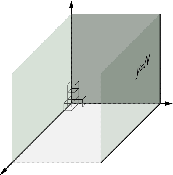
(a) (b)

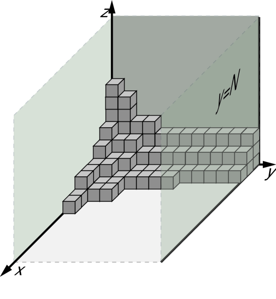
Figure 1: (a) The crystal melting model for the resolved conifold ${\mathcal{O}}(-1)\oplus{\mathcal{O}}(-1)\rightarrow{\bf P}^{1}$. The edges, drawn as solid lines, of the positive octant bounded by the wall at $y=N$ form the toric diagram of the resolved conifold. (b) Many atoms have been removed from the crystal. Atoms cannot be removed from the region beyond the wall at $y=N$.

Now we demonstrate that this crystal melting program indeed reproduces the partition function for the resolved conifold. For this purpose, we express the partition function in terms of free fermions and bosons:

$$\psi(z)=\sum_{r\in{\bf Z}+1/2}\frac{\psi_{r}}{z^{r+1/2}},~{}\bar{\psi}(z)=\sum_{r}\frac{\bar{\psi}_{r}}{z^{r+1/2}},$$ (2.2)

$$\{\psi_{r},\bar{\psi}_{s}\}=\delta_{r+s,0},$$ (2.3)

$$\phi(z)=x_{0}-i\alpha_{0}\log z+i\sum_{n\neq 0}\frac{\alpha_{n}}{nz^{n}},$$ (2.4)

$$\left[\alpha_{m},\alpha_{n}\right]=m\delta_{m+n,0}.$$ (2.5)

These are related via

$$i\partial\phi(z)=:\psi\bar{\psi}(z):,~{}~{}\psi(z)=:e^{i\phi(z)}:,~{}~{}\bar{\psi}(z)=:e^{-i\phi(z)}:.$$ (2.6)

Now we define

$$\Gamma_{\pm}(z)=\exp\sum_{n>0}\frac{z^{\pm n}}{n}\alpha_{\pm n}.$$ (2.7)

It is well known that neutral (zero momentum in the bosonic language) fermionic Fock states are labelled by (2D) Young diagrams $\mu$ which we denote as $\mu=(\mu_{1}\geq\mu_{2}...\geq\mu_{d}>0)$. More explicitly, such Fock states are given by

$$|\mu\rangle = \prod_{i=1}^{\infty}\psi_{i-\mu_{i}-1/2}|0\rangle\rangle$$ (2.8)

$$= \prod_{i=1}^{d}\bar{\psi}_{-a_{i}}\psi_{-b_{i}}|0\rangle,$$

where $|0\rangle\rangle$ is the state that is annihilated by all $\bar{\psi}_{r},r\in{\bf Z}+1/2$, and we have defined

$$a_{i}=\mu_{i}-i+1/2,~{}~{}b_{i}=\mu^{t}_{i}-i+1/2.$$ (2.9)

$\mu^{t}$ is the transposed Young diagram. The Virasoro zero mode $L_{0}$ counts the number $|\mu|$ of boxes in the Young diagram $\mu$:

$$L_{0}|\mu\rangle=|\mu||\mu\rangle.$$ (2.10)

Two Young diagrams $\lambda$ and $\mu$ are said to interlace (and we write $\lambda\succ\mu$) if they satisfy

$$\lambda_{1}\geq\mu_{1}\geq\lambda_{2}\geq\mu_{2}\geq...$$ (2.11)

In other words, $\lambda$ and $\mu$ interlace if and only if $\lambda$ contains $\mu$ and $\mu$ contains $\lambda$ with the first row removed. The interlacing condition is equivalent to the local condition for two Young diagrams one finds by slicing the allowed configuration of the crystal by the planes $x=y+j$ and $x=y+j+1$ [3]. The operators $\Gamma_{\pm}(z)$ are useful because of the properties

$$\Gamma_{+}(1)|\lambda\rangle=\sum_{\lambda\succ\mu}|\mu\rangle,$$

$$\Gamma_{-}(1)|\lambda\rangle=\sum_{\mu\succ\lambda}|\mu\rangle.$$ (2.12)

The partition function for the crystal can be written as

$$Z_{\rm crystal}(q,t=g_{s}N)=\langle 0|\left(\prod_{n=1}^{\infty}q^{L_{0}}\Gamma_{+}(1)\right)q^{L_{0}}\left(\prod_{m=1}^{N}\Gamma_{-}(1)q^{L_{0}}\right)|0\rangle$$ (2.13)

$$= \langle 0|\prod_{n=1}^{\infty}\Gamma_{+}(q^{n-1/2})\prod_{m=1}^{N}\Gamma_{-}(q^{-(m-1/2)})|0\rangle.$$

This can be understood as slicing the crystal by planes $x=y+j,j\in{\bf Z}$. Note that we have a finite product of vertex operators acting on $|0\rangle$. This restricts a 3D Young diagram to have a trivial 2D Young diagram on the slice $x=y-N$. The interlacing conditions then imply that the 2D Young diagrams must have at most one row on the slice $x=y-N+1$, two rows on $x=y-N+2$, etc. Thus the free field correlator represents a crystal model bounded by a wall at $y=N$. See figure 2(a).

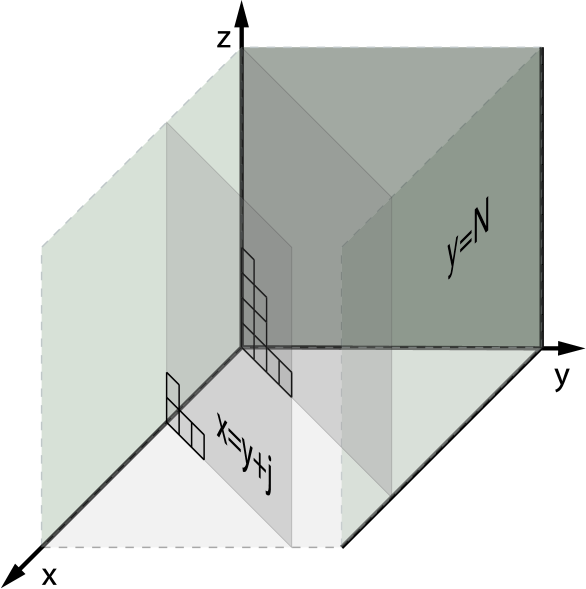
(a) (b)

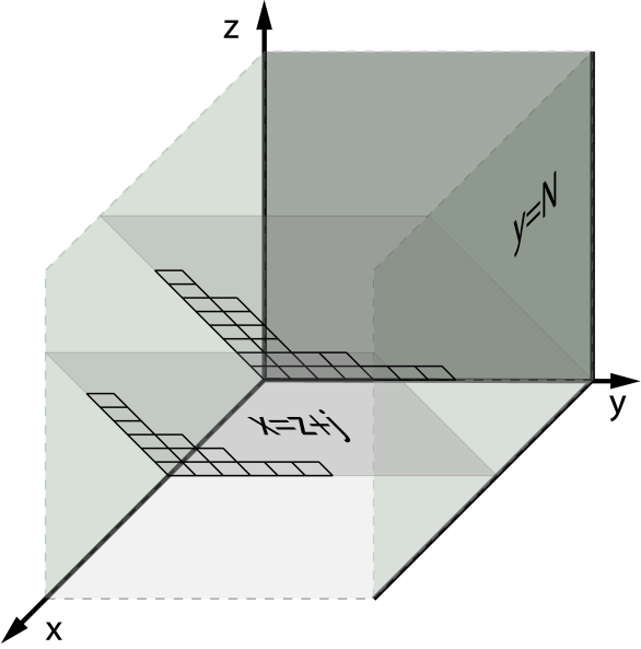
Figure 2: (a)Closed string slicing: This slicing by planes $x=y+j$ allows one to compute the closed string amplitude as in eq. (2.14). (b)Open string slicing: Another slicing of the crystal by planes $x=z+j$ corresponds to the free field representation eq. (3.15) obtained from Chern-Simons theory.

Now we can explicitly compute the partition function.

$$Z_{\rm crystal}(q,t=g_{s}N) = \langle 0|e^{-\sum_{n>0}\frac{\alpha_{n}}{n[n]}}e^{-\sum_{n>0}\frac{1-q^{Nn}}{n[n]}\alpha_{-n}}|0\rangle$$ (2.14)

$$= e^{\sum_{n>0}\frac{1-q^{Nn}}{n[n]^{2}}}$$

$$= M(q)e^{-\sum_{n>0}\frac{e^{-nt}}{n[n]^{2}}}.$$

Taking $N\rightarrow\infty$ pushes the wall at $y=N$ to infinity, and the partition function reduces to the result for ${\bf C}^{3}$.

This crystal model and the resulting amplitude are different from those discussed in [4]. While our crystal has a fixed finite size in the $y$ direction, in [4] the distance between the two crystal corners are not fixed because two finite size 3D partitions are connected through a region of length $t=g_{s}N$. Consequently, in stead of a single power of $M(q)$ in our model, the model [4] gives the square of $M(q)$. More generally, a closed string partition function contains $M(q)^{\chi(X)/2}$, where $\chi(X)$ is the Euler characteristic of the target space $X$. If the target space $X$ is non-compact, the definition of the Euler characteristic is ambiguous. In the context of large $N$ duality, it is known [8] that one should assign the value 2 to the Euler characteristic of the resolved conifold as we just did. This is natural in the sense that the target space admits one Kähler deformation but no complex structure deformation, and the general formula for a (compact) Calabi-Yau manifold is $\chi(X)=2\left[(\#{\rm K\ddot{a}hler~{}deformations})-(\#{\rm Complex~{}structure~{}deformations})\right]$.

3 Large $N$ dual open string theory

In this section, we study the crystal melting problem from the point of view of large $N$ duality.

The crystal model in the previous section can also be expressed as

$$Z_{\rm crystal}(q,t=g_{s}N)$$ (3.15)

$$= \langle 0|\prod_{n=1}^{\infty}\Gamma_{+}(q^{n-1/2}){\bf 1}_{d^{t}\leq N}\prod_{m=1}^{\infty}\Gamma_{-}(q^{-(m-1/2)})|0\rangle$$

Here ${\bf 1}_{d^{t}\leq N}$ is the operator that projects onto the subspace spanned by $|\mu\rangle$ such that the Young diagram $\mu$ has at most $N$ columns. This free field expression corresponds to slicing the crystal by planes $z-x=j,j\in{\bf Z}$. See figure 2(b).

We call this the “open string slicing” because, as we will see below, this representation of the crystal naturally arises from Chern-Simons theory.

3.1 Unitary matrix model for Chern-Simons theory

The large $N$ duality of Gopakumar and Vafa relates $U(N)$ Chern-Simons theory on $S^{3}$ to topological closed string on the resolved conifold ${\mathcal{O}}(-1)\oplus{\mathcal{O}}(-1)\rightarrow{\bf P}^{1}$. The dictionary is that the Kähler modulus $t$ of the closed string theory geometry is identified with the ’t hooft parameter $g_{s}N$. Certain amplitudes on the resolved conifold, including the closed string amplitudes, can be computed within the framework of Chern-Simons theory. We now develop a unitary matrix model formulation of Chern-Simons theory, which will be used to derive the crystal model for the resolved conifold later.

The partition function of the $U(N)$ Chern-Simons theory on $S^{3}$ is given by [9]

$$Z_{\rm CS}(N,k,U(N)) = \frac{1}{(k+N)^{N/2}}\prod_{\alpha>0}2\sin\frac{\pi\alpha\cdot\rho}{k+N}.$$ (3.16)

Here $2\pi i/(k+N)=g_{s}$ is the string coupling constant, and the product is over the positive roots of $SU(N)\subset U(N)$ which are given by $\alpha_{ij}=e_{i}-e_{j}\in{\bf C}^{N}$($\simeq$ Cartan subalgebra) for $i<j$. $\rho=(1/2)\sum_{\alpha>0}\alpha=\sum_{i=1}^{N}(\frac{N+1}{2}-i)e_{i}$ is the Weyl vector. Now note the following formula by Weyl for the denominator of the Lie algebra characters

$$\prod_{\alpha>0}2\sinh(\alpha\cdot u)=\sum_{w\in W}\epsilon(w)e^{w(\rho)\cdot u},$$ (3.17)

where $W$ is the Weyl group isomorphic to the permutation group $S_{N}$ and $u$ is an arbitrary element of the Cartan subalgebra of $U(N)$. We use this identity to rewrite $Z_{\rm CS}(N,k,U(N))=:Z_{\rm CS}(g_{s},N)$ as

$$Z_{\rm CS}(g_{s},N) = \frac{e^{-\frac{N(N-1)\pi i}{4}}}{(k+N)^{N/2}}\sum_{w\in W}\epsilon(w)e^{g_{s}w(\rho)\cdot\rho}$$ (3.18)

$$= \left(\frac{g_{s}}{2\pi}\right)^{N/2}e^{-\frac{\pi i}{4}N^{2}}q^{-\frac{N(N-1)}{12}}\tilde{Z}_{\rm CS}(g_{s},N)$$

Here we have factored out the non-trivial part of the partition function:

$$\tilde{Z}_{\rm CS}(g_{s},N)=\sum_{w\in W}\epsilon(w)q^{\frac{1}{2}(w(\rho)-\rho)^{2}}.$$ (3.19)

$q$ is again $e^{-g_{s}}$. In what follows, we “analytically continue” in $g_{s}$ and regard $g_{s}$ as a complex parameter with a positive real part. We can introduce another sum over the Weyl group and an integral over the maximal torus as follows:

$$\tilde{Z}_{\rm CS}(g_{s},N)$$ (3.20)

$$= \frac{1}{|W|}\sum_{w,w^{\prime}\in W}\epsilon(w)\epsilon(w^{\prime})q^{\frac{1}{2}(w(\rho)-w^{\prime}(\rho))^{2}}$$

$$= \frac{1}{|W|}\int\prod_{i=1}^{N}\left(\frac{d\theta_{i}}{2\pi}\vartheta_{00}(e^{i\theta_{i}};q)\right)\sum_{w,w^{\prime}\in W}\epsilon(w)\epsilon(w^{\prime})e^{i(w(\rho)-w^{\prime}(\rho))\cdot\theta}.$$

Here

$$\vartheta_{00}(e^{i\theta};q):=\sum_{m\in{\bf Z}}q^{\frac{m^{2}}{2}}e^{im\theta}$$ (3.21)

is one of Jacobi’s theta functions.

By making use of the Weyl denominator formula eq. (3.17) again, we get

$$\tilde{Z}_{\rm CS} = \frac{1}{|W|}\int\left(\prod_{i=1}^{N}\frac{d\theta_{i}}{2\pi}\vartheta_{00}(e^{i\theta_{i}})\right)\left(\prod_{\alpha>0}2\sin\frac{\alpha\cdot\theta}{2}\right)^{2}.$$ (3.22)

The second factor now represents the Haar measure for $U(N)$ pushed down to the maximal torus. The partition function can be written in a very simple form

$$\tilde{Z}_{\rm CS}=\int_{U(N)}dU\det\vartheta_{00}(U;q),$$ (3.23)

where the measure is normalized so that the volume of $U(N)$ is unity. This expression holds for any gauge group of the Chern-Simons theory on $S^{3}$ when the corresponding Haar measure is used.

3.2 Crystal from Chern-Simons theory

Now we use the product formula for the theta function

$$\vartheta_{00}(e^{i\theta};q) = \prod_{j=1}^{\infty}(1-q^{j})(1+e^{i\theta}q^{j-1/2})(1+e^{-i\theta}q^{j-1/2})$$ (3.24)

$$= \left(\prod_{j=1}^{\infty}(1-q^{j})\right)\exp\left[\sum_{n>0}(-1)^{n}\frac{e^{in\theta}+e^{-in\theta}}{n[n]}\right]$$

to write

$$\tilde{Z}_{\rm CS} = \left(\prod_{j=1}^{\infty}(1-q^{j})\right)^{N}\int dU\exp\left[\sum_{n>0}(-1)^{n}\frac{{\rm Tr}U^{n}+{\rm Tr}U^{-n}}{n[n]}\right]$$ (3.25)

$$= \left(\prod_{j=1}^{\infty}(1-q^{j})\right)^{N}\int dU\exp\left[\sum_{n>0}\frac{{\rm Tr}U^{n}+{\rm Tr}U^{-n}}{n[n]}\right]$$

To obtain the free-field expression for the partition function, we introduce the coherent states:

$$|U\rangle:=\exp\left[\sum_{n>0}\frac{1}{n}{\rm Tr}~{}U^{n}\alpha_{-n}\right]|0\rangle.$$ (3.26)

These states satisfy

$$\alpha_{n}|U\rangle={\rm Tr}~{}U^{n}|U\rangle,$$ (3.27)

$$\int dU|U\rangle\langle U|={\bf 1}_{d\leq N},$$ (3.28)

where ${\bf 1}_{d\leq N}$ is the projection to the subspace spanned by $|\mu\rangle$ such that the number of rows in $\mu$ is less than or equal to $N$. This formalism was extensively used in the context of 2D Yang-Mills theory which has recently been attracting some attention [12, 13, 14]. See [15] and the references therein.

By making use of $|U\rangle$, we can write

$$\tilde{Z}_{\rm CS} = \left(\prod_{j=1}^{\infty}(1-q^{j})\right)^{N}\langle 0|e^{\sum_{n>0}\frac{\alpha_{n}}{n[n]}}\int dU|U\rangle\langle U|e^{\sum_{n>0}\frac{\alpha_{-n}}{n[n]}}|0\rangle$$ (3.29)

$$= \left(\prod_{j=1}^{\infty}(1-q^{j})\right)^{N}\langle 0|e^{\sum_{n>0}\frac{\alpha_{n}}{n[n]}}{\bf 1}_{d\leq N}e^{\sum_{n>0}\frac{\alpha_{-n}}{n[n]}}|0\rangle$$

Since $\alpha_{n}\rightarrow-\alpha_{n}$ is equivalent to $R\rightarrow R^{t}$ (c.f. eq. (2.8)), we finally obtain

$$\tilde{Z}_{\rm CS} = \left(\prod_{j=1}^{\infty}(1-q^{j})\right)^{N}\langle 0|e^{-\sum_{n>0}\frac{\alpha_{n}}{n[n]}}{\bf 1}_{d^{t}\leq N}e^{-\sum_{n>0}\frac{\alpha_{-n}}{n[n]}}|0\rangle$$ (3.30)

$$= \xi(q)^{-N}Z_{\rm crystal}(q;t=g_{s}N).$$

We have demonstrated that the open string slicing eq. (3.15) naturally arises from Chern-Simons theory. Note that there is a mismatch by the factor $\xi(q)^{-N}$ between $\tilde{Z}_{\rm CS}$ and $Z_{\rm crystal}$, where $\xi(q)=1/\prod_{j=1}^{\infty}(1-q^{j})$ is the “renormalization factor” which was found in [7] to be associated with a non-compact D-brane. As in [7], we use the modular property of $\eta(q)=q^{1/24}\xi(q)^{-1}$, namely $\eta(q)=\sqrt{2\pi/g_{s}}\eta(\tilde{q}),\tilde{q}=e^{-4\pi^{2}/g_{s}}$, to argue that it does not contribute to the perturbative amplitudes at genus no less than $2$ when comparing the open and closed string sides. For genus amplitudes, the mismatch is absorbed into the usual ambiguities.

4 Adding D-branes

We can add non-compact D-branes to the system. In the language of Chern-Simons gauge theory, this corresponds to placing Wilson lines going through circles of links. In the case of an unknot, we will be able to see the connection to the description in [7].

On the open string side, we consider placing a stack of $M$ non-compact D-branes in $T^{\ast}S^{3}$ intersecting the $S^{3}$ along an unknot $S^{1}$ [16]. Since the new D-branes are non-compact, we treat them as non-dynamical, acting as a source to the gauge fields on $S^{3}$ via an interaction. This interaction is obtained by integrating out the degrees freedom coming from the open strings stretching between the compact D-branes wrapping the $S^{3}$ and the non-compact D-branes. Let $U\in U(N)$ and $V\in U(M)$ be the holonomies along the unknot for the gauge fields on the compact and the non-compact D-branes, respectively. Then the interaction can be represented as

$$\int{\mathcal{D}}Ae^{-S_{CS}[A]+\sum_{n=1}^{\infty}\frac{1}{n}{\rm Tr}U^{n}{\rm Tr}V^{n}}=Z_{CS}(S^{3})\langle e^{\sum_{n=1}^{\infty}\frac{1}{n}{\rm Tr}U^{n}{\rm Tr}V^{n}}\rangle.$$ (4.31)

The expectation value can be expanded, with the help of Frobenius’ formula, as

$$\langle e^{\sum_{n=1}^{\infty}\frac{1}{n}{\rm Tr}U^{n}{\rm Tr}V^{n}}\rangle = \sum_{\mu}\langle{\rm Tr}_{\mu}U\rangle{\rm Tr}_{\mu}V.$$ (4.32)

Here ${\rm Tr}_{\mu}$ denotes the trace in the representation of $U(N)$ or $U(M)$ specified by the Young diagram $\mu$.

It is natural to expect that $\langle{\rm Tr}_{\mu}U\rangle$ in eq. (4.32) is computed by the unitary matrix model in subsection 3.1 by inserting ${\rm Tr}_{\mu}U$. We now show that this is indeed correct, however with the subtlety that the Wilson line and hence the non-compact D-branes have non-canonical framing.

The object we would like to compute is

$$\int dU\det\vartheta_{00}(U;q){\rm Tr}_{\mu}U.$$ (4.33)

Going back to the eigenvalue integral, this is

$$\int\prod_{i=1}^{N}\frac{d\theta_{i}}{2\pi}\vartheta_{00}(e^{i\theta_{i}})\det\left[(e^{i\theta_{j}})^{N-i}\right]\det\left[(e^{-i\theta_{j}})^{N-i}\right]\frac{\det\left[(e^{i\theta_{j}})^{\mu_{i}+N-i}\right]}{\det\left[(e^{i\theta_{j}})^{N-i}\right]},$$ (4.34)

where we have used the Jacobi-Trudy formula ${\rm Tr}_{\mu}{\rm diag}(x_{1},...,x_{N})\equiv s_{\mu}(x_{1},...,x_{N})=\det x_{j}^{\mu_{i}+N-i}/\det x_{j}^{N-i}$ for the Schur polynomial. After cancelling factors between the numerator and the denominator, and performing the integrals the matrix integral reduces to

$$\frac{1}{N!}\sum_{\sigma,\sigma^{\prime}\in S_{N}}{\rm sgn}\sigma~{}{\rm sgn}\sigma^{\prime}\prod_{j=1}^{N}q^{\frac{1}{2}\left(\mu_{\sigma(j)}-\sigma(j)+\sigma^{\prime}(j)\right)^{2}}$$ (4.35)

$$= \sum_{\sigma\in S_{N}}{\rm sgn}\sigma\prod_{j=1}^{N}q^{\frac{1}{2}\left(\mu_{j}-j+\sigma(j)\right)^{2}}$$

$$= \det\left[q^{\frac{1}{2}(\mu_{i}-i+j)^{2}}\right].$$

Up to $\mu$-independent factors, this equals

$$q^{\frac{1}{2}\sum_{i=1}^{N}\mu_{i}(\mu_{i}-2i+N+1)}\det\left[q^{(j-\frac{N+1}{2})(\mu_{i}-i+N)}\right].$$ (4.36)

The power of $q$ can be written as $q^{(\kappa_{\mu}+N|\mu|)/2}$, where $\kappa_{\mu}=2\sum_{(i,j)\in\mu}(i-j)=\sum_{i}\mu_{i}(\mu_{i}-2i+1)$. This is the factor one obtains when the framing of the Wilson loop is shifted by one unit [9]. The determinant is of the form that appears in the numerator of the Jacobi-Trudy formula. Hence we have shown that

$$\frac{\int dU\det\vartheta_{00}(U;q){\rm Tr}_{\mu}U}{\int dU\det\vartheta_{00}(U;q)}$$ (4.37)

$$= q^{(\kappa_{\mu}+N|\mu|)/2}{\rm Tr}_{\mu}{\rm diag}(q^{-\frac{N-1}{2}},q^{-\frac{N-3}{2}},...,q^{\frac{N-1}{2}}).$$

Relative to the result for the canonically framed unknot [16], we see that the matrix model computes amplitudes in the framing shifted by one unit.

This vacuum expectation value of the Wilson loop can be represented as a crystal melting model as follows.

$$\int dU\det\vartheta_{00}(U;q){\rm Tr}_{\mu}U$$ (4.38)

$$= \xi(q)^{-N}\langle 0|e^{\sum_{n>0}\frac{\alpha_{n}}{n[n]}}\int dU{\rm Tr}_{\mu}U|U\rangle\langle U|e^{\sum_{n>0}\frac{\alpha_{-n}}{n[n]}}|0\rangle$$

$$= \xi(q)^{-N}\langle 0|e^{\sum_{n>0}\frac{\alpha_{n}}{n[n]}}\int dU\sum_{\vec{k}}\frac{1}{z_{\vec{k}}}\chi_{\mu}(C(\vec{k}))\prod_{j=1}^{\infty}\alpha_{j}^{k_{j}}|U\rangle\langle U|e^{\sum_{n>0}\frac{\alpha_{-n}}{n[n]}}|0\rangle,$$

where $\chi_{\mu}$ is the $S_{|\mu|}$ character of the representation specified by $\mu$, $\vec{k}=(k_{1},k_{2},...)$ is an infinite vector with non-negative integer components, and $C(\vec{k})$ is the conjugacy class of $S_{|\mu|}$ specified by $\vec{k}$. Now the powers of $\alpha_{j}$ can be moved to the left to act on $\langle 0|$. This yields

$$\int dU\det\vartheta_{00}(U;q){\rm Tr}_{\mu}U$$ (4.39)

$$= \xi(q)^{-N}\langle\mu|e^{\sum_{n>0}\frac{\alpha_{n}}{n[n]}}\int dU|U\rangle\langle U|e^{\sum_{n>0}\frac{\alpha_{-n}}{n[n]}}|0\rangle$$

$$= \xi(q)^{-N}\langle\mu|e^{\sum_{n>0}\frac{\alpha_{n}}{n[n]}}{\bf 1}_{d\leq N}e^{\sum_{n>0}\frac{\alpha_{-n}}{n[n]}}|0\rangle$$

$$= \xi(q)^{-N}\langle\mu^{t}|e^{-\sum_{n>0}\frac{\alpha_{n}}{n[n]}}{\bf 1}_{d^{t}\leq N}e^{-\sum_{n>0}\frac{\alpha_{-n}}{n[n]}}|0\rangle$$

$$= \xi(q)^{-N}\langle\mu^{t}|\prod_{n=1}^{\infty}\Gamma_{+}(q^{n-1/2}){\bf 1}_{d^{t}\leq N}\prod_{m=1}^{\infty}\Gamma_{-}(q^{-(m-1/2)})|0\rangle$$

$$= \xi(q)^{-N}q^{\sum_{i=1}^{\infty}(i-1/2)\mu^{t}_{i}}Z_{\rm crystal}^{\rm D-branes},$$

where we have defined

$$Z_{\rm crystal}^{\rm D-branes}:=q^{-\sum_{i=1}^{\infty}(i-1)\mu^{t}_{i}}\langle\mu^{t}|\prod_{n=1}^{\infty}\Gamma_{+}(q^{n}){\bf 1}_{d^{t}\leq N}\prod_{m=1}^{\infty}\Gamma_{-}(q^{-(m-1)})|0\rangle$$ (4.40)

This free field correlator together with the power of $q$ represents, in the open string slicing, the partition function of the crystal melting model whose initial configuration is shown in figure 3. The power of $q$ ensures that the initial configuration has zero energy.

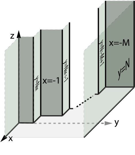
Figure 3: The initial configuration of the crystal with defects representing multiple non-compact D-branes intersecting ${\bf P}^{1}$ in the resolved conifold. The defects introduce faces at $y=\mu^{t}_{1}=N_{1}-M+1,\mu^{t}_{2}=N_{2}-M+2,...,\mu_{M-1}^{t}=N_{M-1}-1,\mu_{M}^{t}=N_{M}$.

It is possible to express the multi-D-brane crystal in the closed string slicing, which is a slight generalization of the free field representation in [7].

$$Z_{\rm crystal}^{\rm D-branes}$$ (4.41)

$$= \langle 0|\prod_{n=1}^{\infty}\Gamma_{+}(q^{n-1/2})\prod_{m=1}^{N_{M}}\Gamma_{-}(q^{-(m-1/2)})\Gamma_{+}(q^{-(N_{M}+1/2)})$$

$$~{}\times\prod_{m=N_{M}+2}^{N_{M-1}}\Gamma_{-}(q^{-(m-1/2)})\Gamma_{+}(q^{-(N_{M-1}+1/2)})\prod_{m=N_{M-1}+2}^{N_{M-2}}\Gamma_{-}(q^{-(m-1/2)})\Gamma_{+}(q^{-(N_{M-2}+1/2)})...$$

$$~{}\times\prod_{m=N_{2}+2}^{N_{1}}\Gamma_{-}(q^{-(m-1/2)})\Gamma_{+}(q^{-(N_{1}+1/2)})\prod_{m=N_{1}+2}^{N+M}\Gamma_{-}(q^{-(m-1/2)})|0\rangle.$$

Here $\mu^{t}_{1}=N_{1}-M+1,\mu^{t}_{2}=N_{2}-M+2,...,\mu_{M-1}^{t}=N_{M-1}-1,\mu_{M}^{t}=N_{M}$. In the closed string slicing, it is possible to explicitly evaluate the correlator to write it as a product. This also provides us with an interpretation of $N_{i}$ as positions of D-branes and exhibits an interesting shift in the Kähler modulus:

$$Z_{\rm crystal}^{\rm D-branes}$$ (4.42)

$$= \left(\prod_{n=1}^{\infty}\prod_{1\leq m\leq N+M,m\neq N_{j}+1}\frac{1}{1-q^{n+m-1}}\right)\prod_{i=1}^{M}\prod_{N_{i}+2\leq m\leq N+M,m\neq N_{j}+1}\frac{1}{1-q^{m-N_{i}-1}}$$

$$= \xi(q)^{M}\left[\prod_{1\leq i<j\leq M}(1-e^{a_{j}-a_{i}})\right]$$

$$~{}~{}\times M(q)\exp\left(-\sum_{n=1}^{\infty}\frac{e^{-n\tilde{t}}}{n[n]^{2}}\right)\prod_{i=1}^{M}\exp\left(\sum_{n=1}^{\infty}\frac{e^{-na_{i}}+e^{-n(\tilde{t}-a_{i})}}{n[n]}\right).$$

Here we have defined $a_{i}:=g_{s}(N_{i}+1/2),~{}i=1,...,M$ and $\tilde{t}:=g_{s}(N+M)=t+g_{s}M$. Again, $\xi(q)$ can be essentially ignored in the perturbative computation due to the modular property of $\eta(q)=q^{1/24}\xi(q)^{-1}$. The second factor $\prod_{i<j}(1-e^{a_{j}-a_{i}})$ is also present in the multi-brane case of [7], and written in this way is independent of $g_{s}$. This is the amplitude for $M$ non-compact D-branes in the resolved conifold, which can be defined as the Kähler quotient

$$\{(X_{I})\in{\bf C}^{4}:|X_{1}|^{2}+|X_{2}|^{2}-|X_{3}|^{2}-|X_{4}|^{2}={\rm Re}~{}\tilde{t}\}/U(1)$$ (4.43)

with $U(1)$ action by charges $(1,1,-1,-1)$. The geometry of the D-branes is [18]

$$|X_{1}|^{2}-{\rm Re}(a_{i})=|X_{2}|^{2}-{\rm Re}~{}(\tilde{t}-a_{i})=|X_{3}|^{2}=|X_{4}|^{2},~{}~{}\sum_{I}\arg X_{I}=0.$$ (4.44)

One thing that is interesting in our computation is that the Kähler parameter is shifted from $t=g_{s}N$ to $\tilde{t}=t+g_{s}M$. It has been known (see, for example, [19]) that the presence of D-branes can shift the effective size of the geometry by the string coupling times the number of D-branes. Here we have found another such phenomenon. The genus zero part of eq. (4.42) in the case of a single D-brane agrees with the results in [20].

The fact that that non-compact D-branes can be nicely incorporated to the crystal confirms that our crystal model of the resolved conifold is a natural one.

5 More general large $N$ dualities, instanton counting, and geometric engineering

So far we have been discussing the Calabi-Yau crystal in the context of Gopakumar-Vafa duality ($T^{\ast}S^{3}\Leftrightarrow{\mathcal{O}}(-1)\oplus{\mathcal{O}}(-1)\rightarrow{\bf P}^{1})$, the simplest example of large $N$ duality in topological string theory. There is a family of generalizations of the large $N$ duality which is worth considering in relation to Calabi-Yau crystal. The example of Gopakumar and Vafa is simple enough to prove the duality (at least at the level of free energies and some open string amplitudes) by direct calculations. However, our derivation of the resolved conifold crystal from Chern-Simons theory can be viewed as a complicated way of proving the duality. In this section we discuss the possible application of the ideas in the present paper to prove more general large $N$ dualities.

Aganagic, Klemm, Marino, and Vafa made a conjecture in [11] that that the duality of Gopakumar and Vafa still holds after taking a ${\bf Z}_{n}$ orbifold on the both sides of duality. On the closed string side, this produces $A$-type topological closed string theory living on the particular fibration of the $A_{n-1}$ ALE space over ${\bf P}^{1}$. The geometry has $n$ Kähler moduli, the sizes of the base ${\bf P}^{1}$ and $n$ additional ${\bf P}^{1}$ that blow up the $A_{n-1}$ singularity. On the open string side, we again get Chern-Simons theory, this time living on the lens space $L(n,1)\simeq S^{3}/{\bf Z}_{n}$. Also after taking the orbifold, the relevant open string theory is a sector of Chern-Simons theory which contains one classical solution. A classical solution can be specified by a holonomy $\exp[2\pi i/N{\rm diag}(\stackrel{{\scriptstyle N_{1}}}{{\overbrace{1,...,1}}},\stackrel{{\scriptstyle N_{2}}}{{\overbrace{2,...,2}}},...,\stackrel{{\scriptstyle N_{n}}}{{\overbrace{n,...,n}}})]$ along the generator of the homotopy group. The Kähler parameters are then to be identified with linear combinations of the t’ Hooft parameters $g_{s}N_{i},i=1,...,n$.

The $n=2$ duality was tested via perturbative computations by the authors who proposed the duality [11]. For general $n$ and a related duality, checks have been done by showing that the matrix models describing the sector of Chern-Simons theory leads to the spectral curves which are the non-trivial parts of the Calabi-Yau manifolds mirror to the A-model closed string geometries [21, 22, 23]. The worldsheet derivation of the Gopakumar-Vafa duality [24] has also been generalized for these large $N$ dualities [25].

There are $n+1$ choices ($m=0,1,...,n+1$ in the notation of [26]) one can make when one fibers the $A_{n-1}$ ALE space over ${\bf P}^{1}$. The closed string geometry that is dual to the $S^{3}/{\bf Z}_{n}$ Chern-Simons theory is precisely the fibration $m=0$ [22] that was shown to correspond to Nekrasov’s instanton counting [27, 28] for the 5D $SU(n)$ gauge theory with vanishing Chern-Simons term [29, 4]. (For the correspondence with non-zero Chern-Simons term, see [30].) Nekrasov’s correspondence between topological closed strings and 5D gauge theory has been discussed in [31, 32, 33] by making use of the topological vertex [19]. As discussed in the introduction, the computation via the topological vertex is closely related to the Calabi-Yau crystal. In particular, the computation takes the form of an expansion in $q=e^{-g_{s}}$.

As we saw in the previous section, the Chern-Simons theory also naturally leads to an expansion in $q$. Hence, it is plausible that one will be able to prove the generalized large $N$ dualities to all order in $g_{s}$ by proving that the partition functions are the same on the both sides as functions of $q$ [34].

Let us also make an observation on the appearance of the unitary matrix model. In [35], the question of finding matrix models that compute the Seiberg-Witten solutions of ${\mathcal{N}}=2$ gauge theories was addressed. The matrix models in [11] can be regarded as computing amplitudes in the 5D gauge theories with the same number of supercharges. By taking a double scaling limit, which is the familiar field theory limit of geometric engineering [36], one can compute amplitudes for 4D ${\mathcal{N}}=2$ gauge theories from these matrix models. By using the technique in this paper, it is possible to rewrite the matrix models in [11] as unitary matrix models. These are similar to, and can be regarded as generalizations of, the unitary matrix model (Gross-Witten one plaquette model [37]) that was considered in [35] for the $SU(2)$ gauge theory.

References

• [1] E. Witten, “Chern-Simons gauge theory as a string theory,” Prog. Math. 133 (1995) 637–678, hep-th/9207094.
• [2] M. Bershadsky, S. Cecotti, H. Ooguri, and C. Vafa, “Kodaira-Spencer theory of gravity and exact results for quantum string amplitudes,” Commun. Math. Phys. 165 (1994) 311–428, hep-th/9309140.
• [3] A. Okounkov, N. Reshetikhin, and C. Vafa, “Quantum Calabi-Yau and classical crystals,” hep-th/0309208.
• [4] A. Iqbal, N. Nekrasov, A. Okounkov, and C. Vafa, “Quantum foam and topological strings,” hep-th/0312022.
• [5] D. Maulik, N. Nekrasov, A. Okounkov, and R. Pandharipande, “Gromov-Witten theory and Donaldson-Thomas theory, I,” math.AG/0312059.
• [6] D. Maulik, N. Nekrasov, A. Okounkov, and R. Pandharipande, “Gromov-Witten theory and Donaldson-Thomas theory, II,” math.AG/0406092.
• [7] N. Saulina and C. Vafa, “D-branes as defects in the Calabi-Yau crystal,” hep-th/0404246.
• [8] R. Gopakumar and C. Vafa, “On the gauge theory/geometry correspondence,” Adv. Theor. Math. Phys. 3 (1999) 1415–1443, hep-th/9811131.
• [9] E. Witten, “Quantum field theory and the Jones polynomial,” Commun. Math. Phys. 121 (1989) 351.
• [10] M. Marino, “Chern-Simons theory, matrix integrals, and perturbative three-manifold invariants,” hep-th/0207096.
• [11] M. Aganagic, A. Klemm, M. Marino, and C. Vafa, “Matrix model as a mirror of Chern-Simons theory,” JHEP 02 (2004) 010, hep-th/0211098.
• [12] C. Vafa, “Two dimensional Yang-Mills, black holes and topological strings,” hep-th/0406058.
• [13] S. de Haro and M. Tierz, “Brownian motion, Chern-Simons theory, and 2d Yang-Mills,” hep-th/0406093.
• [14] S. de Haro, “Chern-Simons theory in lens spaces from 2d Yang-Mills on the cylinder,” JHEP 08 (2004) 041, hep-th/0407139.
• [15] S. Cordes, G. W. Moore, and S. Ramgoolam, “Lectures on 2-d Yang-Mills theory, equivariant cohomology and topological field theories,” Nucl. Phys. Proc. Suppl. 41 (1995) 184–244, hep-th/9411210.
• [16] H. Ooguri and C. Vafa, “Knot invariants and topological strings,” Nucl. Phys. B577 (2000) 419–438, hep-th/9912123.
• [17] J. Fulton and W. Harris, Representation Theory. A First Course. Graduate Texts in Mathematics Vol. 129. Springer-Verlag, 1999.
• [18] M. Aganagic, A. Klemm, and C. Vafa, “Disk instantons, mirror symmetry and the duality web,” Z. Naturforsch. A57 (2002) 1–28, hep-th/0105045.
• [19] M. Aganagic, A. Klemm, M. Marino, and C. Vafa, “The topological vertex,” hep-th/0305132.
• [20] M. Aganagic and C. Vafa, “Mirror symmetry, D-branes and counting holomorphic discs,” hep-th/0012041.
• [21] N. Halmagyi and V. Yasnov, “The spectral curve of the lens space matrix model,” hep-th/0311117.
• [22] N. Halmagyi, T. Okuda, and V. Yasnov, “Large N duality, Lens spaces and the Chern-Simons matrix model,” JHEP 04 (2004) 014, hep-th/0312145.
• [23] V. Yasnov, “Chern-Simons matrix model for local conifold,” hep-th/0409136.
• [24] H. Ooguri and C. Vafa, “Worldsheet derivation of a large N duality,” Nucl. Phys. B641 (2002) 3–34, hep-th/0205297.
• [25] T. Okuda and H. Ooguri, “D branes and phases on string worldsheet,” hep-th/0404101.
• [26] A. Iqbal and A.-K. Kashani-Poor, “SU(N) geometries and topological string amplitudes,” hep-th/0306032.
• [27] N. A. Nekrasov, “Seiberg-Witten prepotential from instanton counting,” Adv. Theor. Math. Phys. 7 (2004) 831–864, hep-th/0206161.
• [28] N. Nekrasov and A. Okounkov, “Seiberg-Witten theory and random partitions,” hep-th/0306238.
• [29] A. Iqbal and A.-K. Kashani-Poor, “Instanton counting and Chern-Simons theory,” Adv. Theor. Math. Phys. 7 (2004) 457–497, hep-th/0212279.
• [30] Y. Tachikawa, “Five-dimensional Chern-Simons terms and Nekrasov’s instanton counting,” JHEP 02 (2004) 050, hep-th/0401184.
• [31] T. Eguchi and H. Kanno, “Topological strings and Nekrasov’s formulas,” JHEP 12 (2003) 006, hep-th/0310235.
• [32] J. Zhou, “Curve counting and instanton counting,” math.AG/0311237.
• [33] T. Eguchi and H. Kanno, “Geometric transitions, Chern-Simons gauge theory and Veneziano type amplitudes,” Phys. Lett. B585 (2004) 163–172, hep-th/0312234.
• [34] T. Okuda. Work in progress.
• [35] R. Dijkgraaf and C. Vafa, “On geometry and matrix models,” Nucl. Phys. B644 (2002) 21–39, hep-th/0207106.
• [36] S. Katz, A. Klemm, and C. Vafa, “Geometric engineering of quantum field theories,” Nucl. Phys. B497 (1997) 173–195, hep-th/9609239.
• [37] D. J. Gross and E. Witten, “Possible third order phase transition in the large N lattice gauge theory,” Phys. Rev. D21 (1980) 446–453.