Six-Quark Amplitudes from Fermionic MHV Vertices

Abstract

The fermionic extension of the CSW approach to perturbative gauge theory coupled with fermions is used to compute the six-quark QCD amplitudes. We find complete agreement with the results obtained by using the usual Feynman rules.

1 Introduction

Recently Witten [1] found a deep connection between the perturbative gauge theory and string theory in twistor space [2]. Based on this work, Cachazo, Svrcek and Witten (CSW for short) reformulated the perturbative calculation of the scattering amplitudes in Yang-Mills theory using the off shell MHV vertices [3]. The MHV vertices are the usual tree level MHV scattering amplitudes in gauge theory [4, 5], continued off shell in a particular fashion as given in [3]. (For references on perturbative calculations, see for example [6]-[10]. The 2 dimensional origin of the MHV amplitudes in gauge theory was first given in [11].) Some sample calculations were done in [3], sometimes with the help of symbolic manipulation. The correctness of the rules was partially verified by reproducing the known results for small number of gluons [6].

In a previous work [12] (for recent works, see [13]-[36]), the extension of the CSW approach to theories with fermions (see also [23]) is discussed and used to calculate the googly fermionic amplitudes. The amplitudes with $3$ quark-anti-quark pairs which are neither MHV nor googly were also analyzed in that paper. In this paper, we will calculate these amplitudes explicitly by using the CSW rules and show that the results are in agreement with the results obtained by using the usual Feynman rules [37]. Although some generic non-MHV fermionic amplitudes were also calculated in [23, 33], we found that it is also worthy to do this calculation. As we will see in the following, the calculation by using the usual Feynman rules is even simpler. So the purpose of our paper is actually to check that the MHV rules are really correct in this non-trivial case.

The MHV (and googly) amplitudes with gluinos or one quark-anti-quark pair can be obtained from the gluonic amplitudes via supersymmetric Ward identities (SWI’s) [38, 39, 6]. But there are more fermionic amplitudes which cannot be obtained in this way. In [40], it has been discussed that neither the non-MHV (googly) amplitudes with gluinos nor the MHV (googly) amplitudes with two quark-anti-quark pairs can be obtained from the gluonic amplitudes by using the SWI’s (See also [33]). In some sense the amplitudes which cannot be obtained via SWI’s have more information. So it is worthy to calculate these amplitudes by using the CSW rules. Although the CSW rule can be partially understood from the twistor string theory [24], a full understanding of the CSW approach from the conventional field theory is not reached [29].

This paper is organized as follows. In section 2, we first review CSW rules for gauge theory without fermions. Then we review extended CSW rules for gauge theory with quarks and the analysis on the CSW diagrams for six-quark amplitudes. In section 3, we calculate the amplitudes with $3$ quark-anti-quark pairs by using the fermionic extension of CSW rules. We show that the result coincides with which from Feynman rules.

2 CSW rules with fermions

First let us review the rules for calculating tree level gauge theory gluonic amplitudes proposed in [3]. Here we follow the presentation given in [13, 14, 12] closely, and consider only partial amplitudes [6]. We will use the convention that all momenta are outgoing. By MHV (with gluons only), we always mean an amplitude with precisely two gluons of negative helicity. If the two gluons of negative helicity are labelled as $r,s$, the MHV vertices are given as follows:

$$V_{n}={\langle\lambda_{r},\lambda_{s}\rangle^{4}\over\prod_{i=1}^{n}\langle\lambda_{i},\lambda_{i+1}\rangle}.$$ (1)

For an on shell (massless) gluon, the momentum in bispinor basis is given as:

$$p_{a\dot{a}}=\sigma^{\mu}_{a\dot{a}}p_{\mu}=\lambda_{a}\tilde{\lambda}_{\dot{a}}.$$ (2)

For an off shell momentum, we can no longer define $\lambda_{a}$ as above. The off-shell continuation given in [3] is to choose an arbitrary spinor $\tilde{\eta}^{\dot{a}}$ and then to define $\lambda_{a}$ as follows:

$$\lambda_{a}=p_{a\dot{a}}\tilde{\eta}^{\dot{a}}.$$ (3)

For an on shell momentum $p$, we will use the notation $\lambda_{pa}$ which is proportional to $\lambda_{a}$:

$$\lambda_{pa}\equiv p_{a\dot{a}}\tilde{\eta}^{\dot{a}}=\lambda_{a}\tilde{\lambda}_{\dot{a}}\tilde{\eta}^{\dot{a}}\equiv\lambda_{a}\phi_{p}.$$ (4)

As demonstrated in [3], it is consistent to use the same $\tilde{\eta}$ for all the off shell momenta. The final result is independent of $\tilde{\eta}$.

By using only MHV vertices, one can build a tree diagram by connecting MHV vertices with propagators. For the propagator of momentum $p$, we assign a factor $1/p^{2}$. The helicity at two ends of a propagator must be opposite. Any possible diagram with the color factor ${\rm Tr}(T^{a_{1}}\cdots T^{a_{n}})$ contributes to the partial amplitude $A_{n}(g_{1}^{h_{1}},\cdots,g_{n}^{h_{n}})$.

Now we review the extension of CSW rules to the gauge theory coupled with quarks and anti-quarks [23, 12]. For this theory we can decompose an amplitude into partial amplitudes with definite color factors [6]. For simplicity we will assume that all quarks have different flavors. When there are identical quarks, the amplitudes can be easily obtained from the amplitudes with distinct quarks. Also we will assume the gauge group to be $U(N)$ instead of $SU(N)$. For a connected diagram with $m$ pair of quark-antiquark, the color factor is

$$(T^{a_{1}}\cdots T^{a_{n_{1}}})_{i_{1}\bar{i_{2}}}(T^{a_{n_{1}+1}}\cdots T^{a_{n_{2}}})_{i_{2}\bar{i_{3}}}\cdots(T^{a_{n_{m-1}+1}}\cdots T^{a_{n}})_{i_{m}\bar{i_{1}}},$$ (5)

for a particular ordering of the quark-antiquarks and gluons [41]. For amplitudes with connected Feynman diagrams, the quark-antiquark color indices $(i,\bar{i})$ must form a ring of length exactly $m$. This can be proved by induction with the number of pairs $m$.

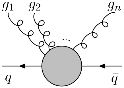
Figure 1: The graphic representation for the single pair of quark-antiquark partial amplitude. Gluons are emitted from one side of the fermion line only.

For a single quark-antiquark pair the color factor is $(T^{a_{1}}\cdots T^{a_{n}})_{i\bar{i}}$. The partial amplitude is denoted as $A_{n+2}(\Lambda^{h}_{q},g_{1},\cdots,g_{n},\Lambda^{-h}_{\bar{q}})$. It is represented as in Fig. 1. We note that gluon lines are emitted only from one side of the (connected) quark-anti-quark line. We will stick to this rule also for multi-pair of quark-antiquark diagrams.

Figure 2: The 2 MHV vertices with quark-antiquarks.

There are 2 MHV vertices with quark-anti-quarks, one for a single pair of quark-antiquark and one for two quark-anti-quark pairs which are shown in Fig. 2. There is no MHV vertex for 3 or more pair of quark-antiquark. All these (non-MHV) amplitudes should be computed from the above MHV vertices by drawing all possible (connected) diagrams with only MHV vertices.

The explicit formulas for these MHV vertices (or amplitudes) are given as follows:

$$V(\Lambda_{q}^{+},g_{1}^{+},\cdots,g_{I}^{-},\cdots,g_{n}^{+},\Lambda_{\bar{q}}^{-})=-{\langle q,I\rangle\langle\bar{q},I\rangle^{3}\over\langle q,1\rangle\langle 1,2\rangle\cdots\langle n,\bar{q}\rangle\langle\bar{q},q\rangle},$$ (6)

$$V(\Lambda_{q}^{-},g_{1}^{+},\cdots,g_{I}^{-},\cdots,g_{n}^{+},\Lambda_{\bar{q}}^{+})={\langle q,I\rangle^{3}\langle\bar{q},I\rangle\over\langle q,1\rangle\langle 1,2\rangle\cdots\langle n,\bar{q}\rangle\langle\bar{q},q\rangle},$$ (7)

for the single pair of quark-antiquark, and for 2 quark-antiquark pairs:

$$\hskip-28.45274ptV(\Lambda_{q_{1}}^{h_{1}},g_{1},\cdots,g_{n_{1}},\Lambda_{\bar{q}_{2}}^{-h_{2}},\Lambda_{q_{2}}^{h_{2}},g_{n_{1}+1},\cdots,g_{n},\Lambda_{\bar{q}_{1}}^{-h_{1}})$$

$$=A_{0}(h_{1},h_{2}){\langle q_{1},\bar{q}_{2}\rangle\over\langle q_{1},1\rangle\langle 1,2\rangle\cdots\langle n_{1},\bar{q_{2}}\rangle}\times{\langle q_{2},\bar{q}_{1}\rangle\over\langle q_{2},n_{1}+1\rangle\cdots\langle n,\bar{q}_{1}\rangle},$$ (8)

where $A_{0}(h_{1},h_{2})$ is given as follows:

$$A_{0}(+,+)={\langle\bar{q}_{1},\bar{q}_{2}\rangle^{2}\over\langle q_{1},\bar{q}_{1}\rangle\langle q_{2},\bar{q}_{2}\rangle}, A_{0}(+,-)=-{\langle\bar{q}_{1},q_{2}\rangle^{2}\over\langle q_{1},\bar{q}_{1}\rangle\langle q_{2},\bar{q}_{2}\rangle},$$ (9)

$$A_{0}(-,+)=-{\langle q_{1},\bar{q}_{2}\rangle^{2}\over\langle q_{1},\bar{q}_{1}\rangle\langle q_{2},\bar{q}_{2}\rangle}, A_{0}(-,-)={\langle q_{1},q_{2}\rangle^{2}\over\langle q_{1},\bar{q}_{1}\rangle\langle q_{2},\bar{q}_{2}\rangle}.$$ (10)

All these MHV amplitudes are given in terms of the “holomorphic” spinors of the external (on-shell) momenta. So we can use the same off shell continuation given in [3] which we recalled above. By including these fermionic MHV vertices, we can extend the CSW rule of perturbative gauge theory to gauge theories with quarks and anti-quarks. The propagator for both gluon and fermion (quark or anti-quark) internal lines is just $1/p^{2}$, as explained in [23]. Helicity is conserved along a fermion line. Because we assume that all quarks have different flavor, the flowing of arrows must follow the directions given exactly in Fig. 2. We use the rules given in [23] to sew vertices by propagators.

Assume that in an MHV diagram, there are $n_{i}$ purely gluonic MHV vertices with $i$ lines, $n_{i}^{2f}$ single pair of quark-antiquark MHV vertices with $(i+2)$ lines (counting also the 2 fermion lines, so actually only $i$ gluon lines), and $n_{i}^{4f}$ 2 pairs of quark-antiquark MHV vertices with $(i+4)$ lines (counting also the 4 fermion lines, so actually only $i$ gluon lines). For a connected diagram with $m$ quark-antiquark pairs, the number of positive helicity gluon $n_{+}$ and the number of negative helicity gluon $n_{-}$ are given as follows [12]:

$$n_{-} = \sum_{i\geq 3}n_{i}+\sum_{i\geq 1}n_{i}^{2f}+\sum_{i\geq 0}n_{i}^{4f}-(m-1),$$ (11)

$$n_{+} = \sum_{i\geq 3}(i-3)\,n_{i}+\sum_{i\geq 1}(i-1)\,n_{i}^{2f}+\sum_{i\geq 0}(i+1)\,n_{i}^{4f}-(m-1).$$ (12)

Figure 3: The 2 different kinds of CSW diagrams contributing to the purely fermionic amplitude with 3 quark-antiquark pairs. In these diagrams $i$ can take $1,2,3$ and the indices are understood as mod $3$. So totally there are $6$ diagrams.

These relations are particularly useful for analyzing diagrams with fewer number of external gluons with positive helicity. For the purely fermionic amplitudes with $3$ quark-antiquark pairs, there are only $2$ different kinds of diagrams as shown in Fig. 3 [12]. By using the extended CSW rules, the partial amplitude can be written down very simply. We show in the next section that this gives the right result for the amplitude.

3 The purely fermionic amplitudes with three quark-antiquark pairs

As mentioned in the previous section, we will compute the purely fermionic amplitudes with three distinct (massless) quark-anti-quark pairs. The color factor is $\delta_{i_{1}\bar{i}_{2}}\delta_{i_{2}\bar{i}_{3}}\delta_{i_{3}\bar{i}_{1}}$, for a particular ordering of the quark-antiquarks. The partial amplitude is denoted as $A_{6}(\Lambda_{q_{1}}^{h_{1}},\Lambda_{\bar{q}_{2}}^{-h_{2}},\Lambda_{q_{2}}^{h_{2}},\Lambda_{\bar{q}_{3}}^{-h_{3}},\Lambda_{q_{3}}^{h_{3}},\Lambda_{\bar{q}_{1}}^{-h_{1}})$.

In this section, we will compute these partial amplitudes first by using the CSW rules, then by using the Feynman rules. we will show that these two results coincite up to a phase factor because of the phase convention we used for the vertices and the propagators in the CSW approach.

As mentioned above, in the CSW approach to compute this partial amplitudes, there are only $2$ different kinds of CSW diagrams as shown in Fig. 3. (We note that these CSW diagrams corresponding to the amplitudes with different helicity configurations are the same. This is different from many gluonic amplitudes, where the CSW diagrams corresponding to the amplitudes with different helicity configurations are different.)

There are $8$ kinds of helicity configurations. We can find some relations among these amplitudes with different helicity configurations.

This first relation is:

$$A_{6}(\Lambda_{q_{1}}^{h_{1}},\Lambda_{\bar{q}_{2}}^{-h_{2}},\Lambda_{q_{2}}^{h_{2}},\Lambda_{\bar{q}_{3}}^{-h_{3}},\Lambda_{q_{3}}^{h_{3}},\Lambda_{\bar{q}_{1}}^{-h_{1}})=A_{6}(\Lambda_{q_{2}}^{h_{2}},\Lambda_{\bar{q}_{3}}^{-h_{3}},\Lambda_{q_{3}}^{h_{3}},\Lambda_{\bar{q}_{1}}^{-h_{1}},\Lambda_{q_{1}}^{h_{1}},\Lambda_{\bar{q}_{2}}^{-h_{2}}).$$ (13)

This means that the amplitudes are invariant under the cyclic permutation of the quark-anti-quark pairs.

The second one is the relation between the two amplitudes related by charge conjugation:

$$A_{6}(\Lambda_{q_{1}}^{h_{1}},\Lambda_{\bar{q}_{2}}^{-h_{2}},\Lambda_{q_{2}}^{h_{2}},\Lambda_{\bar{q}_{3}}^{-h_{3}},\Lambda_{q_{3}}^{h_{3}},\Lambda_{\bar{q}_{1}}^{-h_{1}})=-A_{6}(\Lambda_{q^{\prime}_{3}}^{-h_{3}},\Lambda_{\bar{q}^{\prime}_{2}}^{h_{2}},\Lambda_{q^{\prime}_{2}}^{-h_{2}},\Lambda_{\bar{q}^{\prime}_{1}}^{h_{1}},\Lambda_{q^{\prime}_{1}}^{-h_{1}},\Lambda_{\bar{q}^{\prime}_{3}}^{h_{3}}),$$ (14)

where $\lambda_{q^{\prime}_{i}}=\lambda_{\bar{q}_{i}},\lambda_{\bar{q}^{\prime}_{i}}=\lambda_{q_{i}},\tilde{\lambda}_{q^{\prime}_{i}}=\tilde{\lambda}_{\bar{q}_{i}}$,$\tilde{\lambda}_{\bar{q}^{\prime}_{i}}=\tilde{\lambda}_{q_{i}}$.

These relations can be easily verified case by case, either using the CSW rules or using the Feynman rules.

So we only need to consider the case when $h_{1}=h_{2}=h_{3}=-1/2$ and the case when $h_{1}=h_{2}=-1/2,h_{3}=1/2$. Other cases can be obtained from these cases by permutation of the quark-anti-quark pairs and/or charge conjugation transformation.

When $h_{1}=h_{2}=h_{3}=-1/2$, the amplitude is:

$$A^{CSW}_{6}(\Lambda_{q_{1}}^{-},\Lambda_{\bar{q}_{2}}^{+},\Lambda_{q_{2}}^{-},\Lambda_{\bar{q}_{3}}^{+},\Lambda_{q_{3}}^{-},\Lambda_{\bar{q}_{1}}^{+})=\sum_{i=1}^{3}A^{i}+\sum_{i=1}^{3}\tilde{A}^{i},$$ (15)

where

$$A^{i} = -{\langle q_{i},(\bar{q}_{i}\,q_{i})\rangle^{3}\,\langle\bar{q}_{i},(\bar{q}_{i}\,q_{i})\rangle\over\langle\bar{q}_{i},q_{i}\rangle\,\langle q_{i},(\bar{q}_{i}\,q_{i})\rangle\,\langle(\bar{q}_{i}\,q_{i}),\bar{q}_{i}\rangle}\,{1\over(p_{\bar{q}_{i}}+p_{q_{i}})^{2}}$$ (16)

$$\times{\langle q_{i+1},q_{i+2}\rangle^{2}\over\langle\bar{q}_{i+1},q_{i+1}\rangle\,\langle\bar{q}_{i+2},q_{i+2}\rangle}\,{\langle q_{i+2},\bar{q}_{i+1}\rangle\over\langle q_{i+2},(\bar{q}_{i}\,q_{i})\rangle\langle(\bar{q}_{i}\,q_{i}),\bar{q}_{i+1}\rangle}$$

$$= {\langle q_{i},(\bar{q}_{i}\,q_{i})\rangle^{2}\over\langle\bar{q}_{i},q_{i}\rangle}\,{1\over(p_{\bar{q}_{i}}+p_{q_{i}})^{2}}\,{\langle q_{i+1},q_{i+2}\rangle^{2}\over\langle\bar{q}_{i+1},q_{i+1}\rangle\,\langle\bar{q}_{i+2},q_{i+2}\rangle}$$

$$\times{\langle q_{i+2},\bar{q}_{i+1}\rangle\over\langle q_{i+2},(\bar{q}_{i}\,q_{i})\rangle\langle(\bar{q}_{i}\,q_{i}),\bar{q}_{i+1}\rangle},$$

and

$$\tilde{A}^{i} = -{\langle q_{i},(\bar{q}_{i}\,\bar{q}_{i+1})\rangle^{2}\over\langle\bar{q}_{i},q_{i}\rangle\,\langle\bar{q}_{i+1},(\bar{q}_{i}\,q_{i})\rangle}\,{1\over(p_{\bar{q}_{i}}+p_{q_{i}}+p_{\bar{q}_{i+1}})^{2}}$$

$$\times{\langle q_{i+1},q_{i+2}\rangle^{2}\over\langle(\bar{q}_{i+2}\,q_{i+2}),q_{i+1}\rangle\,\langle\bar{q}_{i+2},q_{i+2}\rangle},$$

Here the expression $\langle(ij),k\rangle$ is defined as $\langle\lambda_{p_{i}+p_{j}},\lambda_{k}\rangle$, and the indices are understood mod $3$.

From the momentum conservation we get $\lambda_{q_{i}}\phi_{q_{i}}+\lambda_{\bar{q}_{i}}\phi_{\bar{q}_{i}}+\lambda_{p_{q_{i}}+{p_{\bar{q}_{i}}}}=0$, so $\langle q_{i},(\bar{q}_{i}\,q_{i})\rangle=\phi_{\bar{q}_{i}}\langle\bar{q}_{i},q_{i}\rangle$ then

$${\langle q_{i},(\bar{q}_{i}\,q_{i})\rangle^{2}\over\langle\bar{q}_{i},q_{i}\rangle}\,{1\over(p_{\bar{q}_{i}}+p_{q_{i}})^{2}}={\phi_{\bar{q}_{i}}^{2}\langle\bar{q}_{i},q_{i}\rangle\over(p_{\bar{q}_{i}}+p_{q_{i}})^{2}}={\phi_{\bar{q}_{i}}^{2}\over[\bar{q}_{i},q_{i}]}.$$ (18)

Using this result, we can write $A^{i}$ as

$$A^{i}={\phi_{\bar{q}_{i}}^{2}\over[\bar{q}_{i},q_{i}]}\,{\langle q_{i+1},q_{i+2}\rangle^{2}\over\langle\bar{q}_{i+1},q_{i+1}\rangle\,\langle\bar{q}_{i+2},q_{i+2}\rangle}\,{\langle q_{i+2},\bar{q}_{i+1}\rangle\over\langle q_{i+2},(\bar{q}_{i}\,q_{i})\rangle\langle(\bar{q}_{i}\,q_{i}),\bar{q}_{i+1}\rangle}.$$ (19)

Similarly, when $h_{1}=h_{2}=-1/2,h_{3}=1/2$, the result given by the CSW rules is

$$A^{CSW}_{6}(\Lambda_{q_{1}}^{-},\Lambda_{\bar{q}_{2}}^{+},\Lambda_{q_{2}}^{-},\Lambda_{\bar{q}_{3}}^{-},\Lambda_{q_{3}}^{+},\Lambda_{\bar{q}_{1}}^{+})=\sum_{i=1}^{3}A^{i}+\sum_{i=1}^{3}\tilde{A}^{i}.$$ (20)

Now

$$A^{1}=-{\phi_{\bar{q}_{1}}^{2}\over[\bar{q}_{1},q_{1}]}{\langle q_{2},\bar{q}_{3}\rangle^{2}\over\langle\bar{q}_{2},q_{2}\rangle\,\langle\bar{q}_{3},q_{3}\rangle}{\langle q_{3},\bar{q}_{2}\rangle\over\langle q_{3},(\bar{q}_{1}\,q_{1})\rangle\,\langle(\bar{q}_{1}\,q_{1}),\bar{q}_{2}\rangle},$$ (21)

$$A^{2}=-{\phi_{\bar{q}_{2}}^{2}\over[\bar{q}_{2},q_{2}]}{\langle q_{1},\bar{q}_{3}\rangle^{2}\over\langle\bar{q}_{3},q_{3}\rangle\,\langle\bar{q}_{1},q_{1}\rangle}{\langle q_{1},\bar{q}_{3}\rangle\over\langle q_{1},(\bar{q}_{2}\,q_{2})\rangle\,\langle(\bar{q}_{2}\,q_{2}),\bar{q}_{3}\rangle},$$ (22)

$$A^{3}=-{\phi_{q_{3}}^{2}\over[\bar{q}_{3},q_{3}]}{\langle q_{1},q_{2}\rangle^{2}\over\langle\bar{q}_{1},q_{1}\rangle\,\langle\bar{q}_{2},q_{2}\rangle}{\langle q_{2},\bar{q}_{1}\rangle\over\langle q_{2},(\bar{q}_{3}\,q_{3})\rangle\,\langle(\bar{q}_{3}\,q_{3}),\bar{q}_{1}\rangle},$$ (23)

and

$$\tilde{A}^{1} = {\langle(q_{3}\,\bar{q}_{1}),q_{1}\rangle^{2}\over\langle\bar{q}_{1},q_{1}\rangle\,\langle(\bar{q}_{1}\,q_{1}),q_{3}\rangle}\,{1\over(p_{\bar{q}_{2}}+p_{q_{2}}+p_{\bar{q}_{3}})^{2}}$$

$$\times{\langle q_{2},\bar{q}_{3}\rangle^{2}\over\langle\bar{q}_{2},q_{2}\rangle\,\langle\bar{q}_{3},(\bar{q}_{2}\,q_{2})\rangle},$$

$$\tilde{A}^{2} = {\langle(q_{3}\,\bar{q}_{1}),\bar{q}_{3}\rangle^{2}\over\langle\bar{q}_{3},q_{3}\rangle\,\langle\bar{q}_{1},(\bar{q}_{3}\,q_{3})\rangle}\,{1\over(p_{\bar{q}_{3}}+p_{q_{3}}+p_{\bar{q}_{1}})^{2}}$$

$$\times{\langle q_{1},q_{2}\rangle^{2}\over\langle\bar{q}_{2},q_{2}\rangle\,\langle(\bar{q}_{2}\,q_{2}),q_{1}\rangle},$$

$$\tilde{A}^{3} = {\langle q_{1},(\bar{q}_{1}\,\bar{q}_{2})\rangle^{2}\over\langle\bar{q}_{1},q_{1}\rangle\,\langle\bar{q}_{2},(\bar{q}_{1}\,q_{1})\rangle}\,{1\over(p_{\bar{q}_{1}}+p_{q_{1}}+p_{\bar{q}_{2}})^{2}}$$

$$\times{\langle q_{2},\bar{q}_{3}\rangle^{2}\over\langle\bar{q}_{3},q_{3}\rangle\,\langle(\bar{q}_{3}\,q_{3}),q_{2}\rangle}.$$

Figure 4: The 2 different kinds of Feynman diagrams contributing to the purely fermionic amplitude with 3 quark-antiquark pairs. In the left diagram $j$ can take $1,2,3$ and the indices are understood as mod $3$. So totally there are $4$ diagrams.

Now we will compute this amplitudes by using the Feynman rules . There are four Feynman diagrams as shown in Fig. 4. We will use the helicity trick (see, for example, [8]).

The result for $h_{1}=h_{2}=h_{3}=-1/2$ is

$$A^{Feynman}_{6}(\Lambda_{q_{1}}^{-},\Lambda_{\bar{q}_{2}}^{+},\Lambda_{q_{2}}^{-},\Lambda_{\bar{q}_{3}}^{+},\Lambda_{q_{3}}^{-},\Lambda_{\bar{q}_{1}}^{+})=\sum_{j=1}^{3}A^{j}+\tilde{A},$$ (27)

where

$$A^{j} = -\langle p_{q_{j}}^{-}|{i\over\sqrt{2}}\gamma^{\mu}i\left(p_{q_{j}}^{\rho}+p_{\bar{q}_{j+1}}^{\rho}+p_{q_{j+1}}^{\rho}\right)\gamma_{\rho}{i\over\sqrt{2}}\gamma^{\nu}|p_{\bar{q}_{j}}^{-}\rangle$$ (28)

$$\times\langle p_{q_{j+1}}^{-}|{i\over\sqrt{2}}\gamma_{\mu}|p_{\bar{q}_{j+1}}^{-}\rangle\langle p_{q_{j+2}}^{-}|{i\over\sqrt{2}}\gamma_{\nu}|p_{\bar{q}_{j+2}}^{-}\rangle{-i\over(p_{\bar{q}_{j+1}}+p_{q_{j+1}})^{2}}{-i\over(p_{\bar{q}_{j+2}}+p_{q_{j+2}})^{2}}$$

$$\times{1\over(p_{q_{j}}+p_{\bar{q}_{j+1}}+p_{q_{j+1}})^{2}}$$

$$= i{\langle q_{j},q_{j+1}\rangle\,[\bar{q}_{j},\bar{q}_{j+2}]\over(p_{\bar{q}_{j+1}}+p_{q_{j+1}})^{2}\,(p_{\bar{q}_{j+2}}+p_{q_{j+2}})^{2}\,(p_{q_{j}}+p_{\bar{q}_{j+1}}+p_{q_{j+1}})^{2}}$$

$$\times\left(\langle q_{j},q_{j+2}\rangle\,[q_{j},\bar{q}_{j+1}]+\langle q_{j+1},q_{j+2}\rangle\,[q_{j+1},\bar{q}_{j+1}]\right),$$

and

$$\tilde{A} = -\langle p_{q_{1}}^{-}|{i\over\sqrt{2}}\gamma_{\mu}|p_{\bar{q}_{1}}^{-}\rangle\langle p_{q_{2}}^{-}|{i\over\sqrt{2}}\gamma_{\nu}|p_{\bar{q}_{2}}^{-}\rangle\langle p_{q_{3}}^{-}|{i\over\sqrt{2}}\gamma_{\rho}|p_{\bar{q}_{3}}^{-}\rangle$$ (29)

$$\times{i\over\sqrt{2}}\left(2(k_{\bar{q}_{1}}+k_{q_{1}})_{\rho}\eta_{\mu\nu}+2(k_{\bar{q}_{2}}+k_{q_{2}})_{\mu}\eta_{\nu\rho}+2(k_{\bar{q}_{3}}+k_{q_{3}})_{\nu}\eta_{\rho\mu}\right)$$

$$\times\prod_{j=1}^{3}{-i\over(p_{\bar{q}_{j}}+p_{q_{j}})^{2}}$$

$$= {-i\over\prod_{j=1}^{3}(p_{\bar{q}_{j}}+p_{q_{j}})^{2}}\sum_{k=1}^{3}\langle q_{k},q_{k+1}\rangle\,[\bar{q}_{k},\bar{q}_{k+1}]$$

$$\times\left(\langle\bar{q}_{k},q_{k+2}\rangle\,[\bar{q}_{k},\bar{q}_{k+2}]+\langle q_{k},q_{k+2}\rangle\,[q_{k},\bar{q}_{k+2}]\right).$$

The bras and kets in eqs. (28) and (29) are denoted by the momenta of corresponding particles.

When $h_{1}=h_{2}=-1/2,h_{3}=1/2$, we can similarly obtain the following result by using the Feynman rules,

$$A^{Feynman}_{6}(\Lambda_{q_{1}}^{-},\Lambda_{\bar{q}_{2}}^{+},\Lambda_{q_{2}}^{-},\Lambda_{\bar{q}_{3}}^{-},\Lambda_{q_{3}}^{+},\Lambda_{\bar{q}_{1}}^{+})=\sum_{j=1}^{3}A^{j}+\tilde{A}.$$ (30)

Now

$$A^{1} = i{\langle q_{1},q_{2}\rangle\,[\bar{q}_{1},q_{3}]\over(p_{\bar{q}_{2}}+p_{q_{2}})^{2}\,(p_{\bar{q}_{3}}+p_{q_{3}}^{2})\,(p_{q_{1}}+p_{\bar{q}_{2}}+p_{q_{2}})^{2}}$$ (31)

$$\times\left(\langle q_{1},\bar{q}_{3}\rangle\,[q_{1},\bar{q}_{2}]+\langle q_{2},\bar{q}_{3}\rangle\,[q_{2},\bar{q}_{2}]\right),$$

$$A^{2} = i{\langle q_{2},\bar{q}_{3}\rangle\,[\bar{q}_{2},\bar{q}_{1}]\over(p_{\bar{q}_{3}}+p_{q_{3}})^{2}\,(p_{\bar{q}_{1}}+p_{q_{1}})^{2}\,(p_{q_{2}}+p_{\bar{q}_{3}}+p_{q_{3}})^{2}}$$ (32)

$$\times\left(\langle q_{2},q_{1}\rangle\,[q_{2},q_{3}]+\langle\bar{q}_{3},q_{1}\rangle\,[\bar{q}_{3},q_{3}]\right),$$

$$A^{3} = i{\langle\bar{q}_{3},q_{2}\rangle\,[q_{3},\bar{q}_{1}]\over(p_{\bar{q}_{1}}+p_{q_{1}})^{2}\,(p_{\bar{q}_{2}}+p_{q_{2}})^{2}\,(p_{q_{3}}+p_{\bar{q}_{1}}+p_{q_{1}})^{2}}$$ (33)

$$\times\left(\langle q_{3},q_{1}\rangle\,[q_{3},\bar{q}_{2}]+\langle\bar{q}_{1},q_{1}\rangle\,[\bar{q}_{1},\bar{q}_{2}]\right),$$

and

$$\tilde{A} = -i\left(\langle q_{1},q_{2}\rangle\,[\bar{q}_{1},\bar{q}_{2}]\left(\langle\bar{q}_{3},\bar{q}_{1}\rangle\,[q_{3},\bar{q}_{1}]+\langle\bar{q}_{3},q_{1}\rangle\,[q_{3},q_{1}]\right)\right.$$ (34)

$$\left.+\langle q_{2},\bar{q}_{3}\rangle\,[\bar{q}_{2},q_{3}]\left(\langle q_{1},\bar{q}_{2}\rangle\,[\bar{q}_{1},\bar{q}_{2}]+\langle q_{1},q_{2}\rangle\,[\bar{q}_{1},q_{2}]\right)\right.$$

$$\left.+\langle\bar{q}_{3},q_{1}\rangle\,[q_{3},\bar{q}_{1}]\left(\langle q_{2},q_{3}\rangle\,[\bar{q}_{2},q_{3}]+\langle q_{2},\bar{q}_{3}\rangle\,[\bar{q}_{2},\bar{q}_{3}]\right)\right)$$

$$\times{1\over\sum_{j=1}^{3}(p_{\bar{q}_{j}}+p_{q_{j}})^{2}}.$$

There are the following constrains from the momentum conservation:

$$\sum_{i=1}^{3}\lambda_{q_{i}}^{\alpha}\tilde{\lambda}_{q_{i}}^{\dot{\alpha}}+\sum_{i=1}^{3}\lambda_{\bar{q}_{i}}^{\alpha}\tilde{\lambda}_{\bar{q}_{i}}^{\dot{\alpha}}=0,\,\alpha=1,2,\,\dot{\alpha}=1,2.$$ (35)

From these constrains, we can solve $\tilde{\lambda}_{\bar{q}_{1}}^{\dot{\alpha}}$ and $\tilde{\lambda}_{q_{1}}^{\dot{\alpha}}$ in terms of other $\lambda$’s and $\tilde{\lambda}$’s. The result is

$$\tilde{\lambda}_{\bar{q}_{1}}^{\dot{\alpha}} = -\sum_{i=2}^{3}{\tilde{\lambda}_{q_{i}}^{\dot{\alpha}}\langle\lambda_{q_{i}},\lambda_{q_{1}}\rangle+\tilde{\lambda}_{\bar{q}_{i}}^{\dot{\alpha}}\langle\lambda_{\bar{q}_{i}},\lambda_{q_{1}}\rangle\over\langle\lambda_{\bar{q}_{1}},\lambda_{q_{1}}\rangle},$$

$$\tilde{\lambda}_{q_{1}}^{\dot{\alpha}} = -\sum_{i=2}^{3}{\tilde{\lambda}_{q_{i}}^{\dot{\alpha}}\langle\lambda_{q_{i}},\lambda_{\bar{q}_{1}}\rangle+\tilde{\lambda}_{\bar{q}_{i}}^{\dot{\alpha}}\langle\lambda_{\bar{q}_{i}},\lambda_{\bar{q}_{1}}\rangle\over\langle\lambda_{q_{1}},\lambda_{\bar{q}_{1}}\rangle}.$$ (36)

We noted that we don’t treat $\tilde{\lambda}$ as the complex conjugation of $\lambda$. So in fact, we have use analytic continuation to the spacetime with signature $(2,2)$, after we obtain our result we can go back the Minkowski space. By using these results and with the help of symbolic manipulation, we can find that

$$A^{Feynman}_{6}=-iA^{CSW}_{6},$$ (37)

either in the case when $h_{1}=h_{2}=h_{3}=-1/2$ or in the case when $h_{1}=h_{2}=-1/2,h_{3}=1/2$. From the argument above we know that we can obtain the same result for all of the helicity configurations as promised.

Acknowledgment

We would like to thank Zvi Bern for useful discussion during ichep’04 at Beijing and Chuan-Jie Zhu for suggesting this topic and discussion.

References

• [1] E. Witten, β€œPerturbative Gauge Theory As A String Theory In Twistor Space,” hep-th/0312171.
• [2] R. Penrose, β€œTwistor Algebra,” J. Math. Phys. 8 (1967) 345; β€œThe Central Programme of Twistor Theory,” Chaos, Solitons, and Fractal 10 (1999) 581.
• [3] F. Cachazo, P. Svrcek and E. Witten, β€œMHV Vertices and Tree Amplitudes In Gauge Theory,” JHEP 0409:006 (2004), hep-th/0403047.
• [4] S. Parke and T. Taylor, β€œAn Amplitude For $N$ Gluon Scattering,” Phys. Rev. Lett. 56 (1986) 2459.
• [5] F. A. Behrends and W. T. Giele, β€œRecursive Calculations For Processes With $N$ Gluons,” Nucl. Phys. B306 (1988) 759.
• [6] M. L. Mangano and S. Parke, β€œMultiparton Amplitudes in Guage Theories,” Phys. Rept. 200 (1991) 30.
• [7] Z. Bern, β€œString-Based Perturbative Methods for Gauge Theories,” TASI Lectures, 1992, hep-ph/9304249.
• [8] L. Dixon, β€œCalculating Scattering Amplitudes Efficiently,” TASI Lectures, 1995, hep-ph/9601359.
• [9] Z. Bern, L. Dixon, and D. Kosower, β€œProgress In One-Loop QCD Calculations,” Ann. Rev. Nucl. Part. Sci. 36 (1996) 109, hep-ph/9602280.
• [10] C. Anastasiou, Z. Bern, L. Dixon, and D. Kosower, β€œPlanar Amplitudes In Maximally Supersymmetric Yang-Mills Theory,” Phys.Rev.Lett. 91 (2003) 251602, hep-th/0309040; Z. Bern, A. De Freitas, and L. Dixon, β€œTwo Loop Helicity Amplitudes For Quark Gluon Scattering In QCD and Gluino Gluon Scattering In Supersymmetric Yang-Mills Theory,” JHEP 0306:028 (2003), hep-ph/0304168.
• [11] V. P. Nair, β€œA Current Algebra for Some Gauge Theory Amplitudes,” Phsy. Lett. B214 (1988) 215–218.
• [12] J.-B. Wu and C.-J. Zhu, β€œ MHV Vertices and Fermionic Scattering Amplitudes in Gauge Theory with Quarks and Gluinos,” hep-th/0406146.
• [13] C.-J. Zhu, β€œThe Googly Amplitudes in Gauge theory,” JHEP 0404:032 (2004), hep-th/0403115.
• [14] J.-B. Wu and C.-J. Zhu, β€œMHV Vertices and Scattering Amplitudes in Gauge Theory,” JHEP 0407:032 (2004), hep-th/0406085.
• [15] R. Roiban, M. Spradlin, and A. Volovich, β€œA Googly Amplitude From The $B$ Model In Twistor Space,” JHEP 0404:012 (2004), hep-th/0402016; R. Roiban and A. Volovich, β€œAll Googly Amplitudes From The $B$ Model In Twistor Space,” hep-th/0402121.
• [16] R. Roiban, M. Spradlin, and A. Volovich, β€œ On the Tree-Level S-Matrix of Yang-Mills Theory ,” Phys.Rev. D70 (2004) 026009, hep-th/0403190.
• [17] N. Berkovits, β€œAn Alternative String Theory in Twistor Space for N=4 Super-Yang-Mills,” Phys.Rev.Lett. 93 (2004) 011601, hep-th/0402045.
• [18] N. Berkovits and L. Motl, β€œCubic Twistorial String Field Theory,” J. High Energy Phys. 0404 (2004) 056, hep-th/0403187.
• [19] M. Aganagic and C. Vafa, β€œMirror Symmetry and Supermanifolds,” hep-th/0403192.
• [20] E. Witten, β€œParity Invariance For Strings In Twistor Space,” hep-th/0403199.
• [21] A. Neitzke and C. Vafa,β€œN=2𝑁2N=2 Strings and the Twistorial Calabi-Yau,” hep-th/0402128.
• [22] N. Nekrasov, H. Ooguri and C. Vafa, β€œS-duality and Topological Strings,” hep-th/0403167.
• [23] G. Georgiou and V. V. Khoze, β€œTree Amplitudes in Gauge Theory as Scalar MHV Diagrams,” JHEP 0405 (2004) 070, hep-th/0404072.
• [24] S. Gukov, L. Motl and A. Neitzke, β€œEquivalence of twistor prescriptions for super Yang-Mills,” hep-th/0404085.
• [25] W. Siegel, β€œUntwisting the twistor superstring,” hep-th/0404255.
• [26] S. Giombi, R. Ricci, D. Robles-Llana and D. Trancanelli, ”A Note on Twistor Gravity Amplitudes,” JHEP 0407 (2004) 059, hep-th/0405086.
• [27] A. D. Popov and C. Saemann, β€œOn Supertwistors, the Penrose-Ward Transform and N=4 super Yang-Mills Theory,” hep-th/0405123.
• [28] N. Berkovits and E. Witten, β€œConformal Supergravity in Twistor-String Theory,” JHEP 0408:009 (2004), hep-th/0406051.
• [29] I. Bena, Z. Bern and D. A. Kosower, β€œTwistor-Space Recursive Formulation of Gauge-Theory Amplitudes,” hep-th/0406133.
• [30] D. A. Kosower, β€œNext-to-Maximal Helicity Violating Amplitudes in Gauge Theory,” hep-th/0406175.
• [31] F. Cachazo, P. Svrcek and E. Witten, β€œTwistor Space Structure of One-Loop Amplitudes in Gauge Theory,” hep-th/0406177.
• [32] A.Β D.Β Popov and M.Β Wolf, β€œTopological B-model on weighted projective spaces and self-dual models in four dimensions,” JHEP 0409:007 (2004), hep-th/0406224.
• [33] G. Georgiou, E. W. N. Glover and V. V. Khoze, β€œNon-MHV Tree Amplitudes in Gauge Theory,” JHEP 0407:048 (2004), hep-th/0407027.
• [34] A.Β Brandhuber, B.Β Spence and G.Β Travaglini, β€œOne-loop gauge theory amplitudes in N = 4 super Yang-Mills from MHV vertices,” hep-th/0407214.
• [35] I.Β Bars, β€œTwistor superstring in 2T-physics,” hep-th/0407239.
• [36] Y.Β Abe, V.Β P.Β Nair and M.Β I.Β Park, β€œMultigluon amplitudes, N = 4 constraints and the WZW model,” hep-th/0408191.
• [37] J. F. Gunion and Z. Kunszt, ”Six-Quark Subprocesses in QCD,” Phys. Lett. B176 (1986) 163.
• [38] M. T. Grisaru, H. N. Pendleton and P. van Nieuwenhuizen, β€œSupergravity and the S Matrix,” Phys. Rev. D15(1977) 996.
• [39] M. T. Grisaru and H. N. Pendleton, β€œSome Properties of Scattering Amplitudes in Supersymmetric Theories,” Nucl. Phys. B214(1977) 81.
• [40] M. Mangano and S. J. Parke, β€œQuark-Gluon Amplitudes in the Dual Expansion”, Nucl. Phys. B299 (1988) 673.
• [41] M. Mangano, β€œThe Color Structure of Gluon Emission,” Nucl. Phys. B309 (1988) 461.