Moduli Entrapment with Primordial Black Holes
Nemanja Kaloper^†,, Joachim Rahmfeld^‡, and Lorenzo Sorbo^†,
†Department of Physics, University of California, Davis, CA 95616
^‡Sun Microsystems, Inc., 7777 Gateway Boulevard, Newark, CA 94560
ABSTRACT

We argue that primordial black holes in the early universe can provide an efficient resolution of the Brustein-Steinhardt moduli overshoot problem in string cosmology. When the universe is created near the Planck scale, all the available states in the theory are excited by strong interactions and cosmological particle production. The heavy states are described in the low energy theory as a gas of electrically and magnetically charged black holes. This gas of black holes quickly captures the moduli which appear in the relation between black hole masses and charges, and slows them down with their vevs typically close to the Planck scale. From there, the modulus may slowly roll into a valley with a positive vacuum energy, where inflation may begin. The black hole gas will redshift away in the course of cosmic expansion, as inflation evicts the black holes out of the horizon.

Inflation [1] is at present the best framework for explaining the origin of our universe. However there still are technical difficulties with implementing inflation in fundamental theory. Inflation needs light scalar fields with very flat potentials and positive vacuum energy, which are hard to obtain from first principles. Even if such degrees of freedom are present, there is still the problem of arranging favorable initial conditions [2], which ensure that the vacuum energy controlled by the light scalars dominates over other energy sources in the inflationary patch. One approach towards resolving this problem is the idea of eternal inflation [3, 4, 5] (for a recent review see [6]), which posits that after inflation starts in some regions of a huge “metauniverse” where the environmental conditions favor it, it will produce many universes as big as ours.

Recently, there has been progress in the direction of implementing eternal inflation in string theory. Backgrounds where eternal inflation can occur have been constructed in flux compactifications [7, 8, 9]. These solutions naturally belong to the landscape of string vacua [10, 11, 12, 13]. In fact, many of the older cosmological solutions in supergravity limits of string theory without future singularities [14] could be fitted at the foothills of the landscape, close to the supersymmetric limits. The landscape picture provides for many valleys where inflation can happen, with some of the moduli fields as inflatons. This would realize the old hope that string moduli may be inflatons [15]. However, this approach may also resurrect the moduli overshooting problem, discussed by Brustein and Steinhardt [16]. Depending how they start, the moduli fields may acquire a lot of kinetic energy on the approach towards the inflationary minima and overshoot them, running off towards the supersymmetric regions of weak coupling. There the spacetime decompactifies and new dimensions of space open up. Thus in order to find a phenomenologically viable cosmology, it is essential to find a way to gently lower the moduli to where inflation can occur and the world remains four-dimensional for a long time.

In this framework, the universe may be described as a compact space, with flat or negatively curved spatial slices [17] (see also [18]). It is created close to the Planck scale. Three of the spatial dimensions grew very big during inflation. The modulus which plays the role of the inflaton could start in the inflationary valley of the potential like in topological inflation [9, 17]. However in some regions modulus may have started high up the slope, and normally it would have overshot the minimum as it rolled down; if instead there is enough radiation, the modulus could still get captured in the minimum thanks to the extra cosmological friction [19]. The main ingredient of this mechanism has been observed in string cosmology earlier in [20, 21]. In the backgrounds dominated by conformal matter where $T^{\mu}{}_{\mu}=0$ the source terms arising from the gravitational couplings of the moduli to matter vanish and moduli are quickly kinetically damped [22, 23]. Their energy density dilutes as $\rho_{h}\sim 1/a^{6}$ for the homogeneous mode or as $\rho_{i}\sim 1/a^{4}$ for inhomogeneities [24], where $a$ is the cosmological scale factor. Some aspects of more phenomenologically motivated, but similar, mechanisms have also been discussed in [25, 26, 27].

We will present here a different mechanism for moduli entrapment. The idea is to use the source term coming from the interactions of the moduli with very heavy, nonrelativistic, charged states in the early universe to enhance the attraction of the inflationary basin. To illustrate the mechanism consider the following analogy with a marble and a bathtub. If one drops a marble alongside the steep wall of the bathtub, the marble will have acquired so much kinetic energy that it will fly over any of the small dimples in the tub’s floor and continue rolling around for a long time. However, if the tub is first filled with water, which slowly drains away, then the marble will loose its kinetic energy very rapidly thanks to the interactions with the water molecules. It will be captured quickly in a dimple on the bottom near the place of original impact. Then water will drain away, analogously to the redshifting of the cosmological matter contents, leaving the marble, or the modulus potential, in control of the evolution of the universe. We will show that a gas of heavy states in string theory, described in the low energy supergravity limit as extremal black holes, can enforce the same effect on the runaway moduli of string compactifications. In this way, the gas of black holes, with high initial energy density, can provide a new mechanism for overcoming the Brustein-Steinhardt overshoot problem.

In what follows we will work with a single dilaton-like scalar modulus, assuming that the theory has been compactified to four dimensions already. We believe that the same mechanism can be realized in more complicated scenarios. Then in the approach of [17], the universe emerges somewhere on the landscape with an energy density close to the string scale. We will consider what happens with the regions where the modulus is not immediately placed in the inflationary plateau. Instead it starts far from the minimum along a steep slope and acquires a large kinetic energy. Because the spatial curvature of the universe is either zero or negative, it does not immediately collapse, but expands under the influence of the dominant sources of stress-energy. This separates the flatness problem from the Planck scale physics, and allows for the possibility that inflation may begin well below the Planck scale. At very high energies where the universe is born, strong interactions, and specifically gravitational particle production [28, 29] will excite all the modes in the spectrum of the theory. This includes the heavy states in the theory, with masses above the string scale. When their masses exceed the Planck scale, such states, with some given quantum numbers, are described as BPS black holes in the supergravity limit. Such states are known to locally fix the scalar field vevs on the horizons to values completely independent of the asymptotic geometry [30].

The masses of these states depend explicitly on the expectation value of the scalar at infinity. To see this, recall the example of the BPS black hole solutions in heterotic string theory, described by the bosonic sector of the effective supergravity action [31, 32, 33]

$$S=\int d^{4}x\sqrt{g}\,\frac{e^{-\varphi}}{\ell_{S}{}^{2}}\,\Bigl{(}R+(\partial\varphi)^{2}-\frac{1}{2}F^{2}_{\mu\nu}\Bigr{)}\,.$$ (1)

A generic BPS soliton of (1) is described by an extremal black hole configuration with mass ${\cal M}$, electric charge ${\cal Q}$ and magnetic charge ${\cal P}$, which are related by [31, 32, 33]

$${\cal M}=\frac{1}{2}\,\Bigl{(}|{\cal Q}|e^{\varphi/2}+|{\cal P}|e^{-\varphi/2}\Bigr{)}\,,$$ (2)

where $\varphi$ is the dilaton vev infinitely far away from the hole, determining the asymptotic value of the string coupling $g_{S}=\exp(\varphi/2)$. This parameter is left completely undetermined by the local black hole dynamics. In the supersymmetric limit it is a modulus which can take any value because it is a flat direction of the theory. The charges ${\cal Q}$ and ${\cal P}$ are quantized in the units of the string scale $\sim 1/\ell_{S}$. Similar situation persists for the case of other moduli fields. If, for the sake of simplicity, we assume that all but one of the moduli are stabilized in the compactification to four dimensions (such as in [7, 35]), the effective 4D action which describes the light modes of the theory is, in the Einstein frame, [31]

$$S=\int d^{4}x\sqrt{g}\,\Bigl{(}\frac{R}{2\kappa^{2}}-\frac{1}{2}(\partial\phi)^{2}-\frac{1}{4}e^{-{\tt g}_{2}\kappa\phi}F^{2}_{\mu\nu}\Bigr{)}\,,$$ (3)

where ${\tt g}_{2}$ is the modulus coupling, and $\kappa=1/M_{Pl}$ is the inverse Planck mass in 4D. A generic BPS soliton of the theory (1) is described by an extremal black hole configuration with mass ${\cal M}$, electric charge ${\cal Q}$ and magnetic charge ${\cal P}$. In general, the solutions for the arbitrary charge assignment for ${\cal Q},{\cal P}$ are not known exactly for an arbitrary value of ${\tt g}_{2}$ [31]. However, it is straightforward to solve (3) for the black hole solutions with only electric, or only magnetic charge, in the extremal limit. They are given by zero entropy, zero temperature configurations of the same global structure as those with ${\tt g}_{2}=\sqrt{2}$ [31]. Their masses and charges are related according to

$${\cal M}_{q}=\frac{|{\cal Q}|}{\kappa}e^{{\tt g}_{2}\kappa\phi/2}\,,~{}~{}~{}~{}~{}~{}~{}~{}~{}~{}~{}~{}{\cal M}_{p}=\frac{|{\cal P}|}{\kappa}e^{-{\tt g}_{2}\kappa\phi/2}\,,$$ (4)

where again $\phi$ is the scalar vev infinitely far away from the hole, determining the asymptotic value of the coupling constant $g=\exp({{\tt g}_{2}\kappa\phi/2})$, and can take any value in the supersymmetric limit. In what follows we will work with the models where the Planck scale and the string scale are close together, so that asymptotically $g\sim{\cal O}(1)$, because typically the minima of the nonperturbative scalar modulus potential appear in this regime. Appropriately, as we will see in what follows, the black hole toy model works as a moduli stopper most efficiently precisely in this regime.

The scalar minima in the mass function (2) have prompted a suggestion [36] that moduli could acquire effective potentials generated by the virtual black hole loops, which can stabilize them. This idea is very interesting because it may incorporate some nonperturbative quantum gravity effects, even though is difficult to reliably compute them. We still don’t know quantum gravity Feynman diagrams for black hole states. Instead of following this route, we will focus on a different application of the minima of (2). We will consider an early universe environment where there is a large number of black holes with scalar-dependent masses as in (4). Once there is a net energy density of them, with both electric and magnetic charges, their interactions with the scalar will produce a damping effect, trapping the scalar to vevs of order of the Planck scale (after we normalize the scalar field canonically). The electric charges block the modulus from running off to the strong coupling, where they are heavy, and the magnetic charges block it from going to the weak coupling, where they become heavy. Thus as long as the charges hang around the modulus cannot easily escape to either side. This is akin to the environmentally induced stabilization effects of [25]. In what follows we will only consider the effects of the black hole gas populated with only electric and only magnetic charges. The dyonic solutions should also exist, and contribute as well. However in the regime where we will work, dyons will be generally heavier than monopoles. Because we assume a nearly thermal initial population of heavy states, we expect that the dyon contributions and effects will be exponentially suppressed relative to the monopole states, and we can safely ignore them.

How do we describe this ensemble of black holes? It is well known that the extremal black hole states with like charges can be arranged in static arrays because the electromagnetic repulsions can neutralize the gravitational attraction between them. In the early universe these charges would neither remain static, nor would they all be of the same sign. Gravity respects gauge symmetries and so charge conservation would require the net charge to be zero. In general, the black hole states will be initially produced by strong (gravitational) interactions near the string scale [28, 29] both as “particles” and “antiparticles”, with opposite charges, carrying both electric and magnetic charges. Hence we will approximate their initial abundances by the nearly thermal distribution law, which should be a sensible order of magnitude estimate. Systems of such black holes would be dynamical, since the forces between black holes would not cancel exactly, due to the presence of charges with both signs. Furthermore, outside of the black holes the space would not be in the vacuum, but in a some, roughly thermally, excited state. It is clear by CPT invariance (4) and equivalence principle that both “particles” and “antiparticles” contribute equally to the stress-energy. States from all mass scales will contribute to the total stress-energy. If they meet and annihilate, their energy would be released as relativistic particles, which we will ignore later on. The effect of radiation on cosmological moduli dynamics has already been considered in [20, 21, 19].

While overall unstable, such arrays of black holes may become sufficiently separated so that the cosmic expansion prevents their complete annihilation. In this case, away from the static limit the leading order electromagnetic interactions can be neglected, and the leading order gravitational effects from the charges can be approximated by the stress-energy tensor of the fluid of massive particles [37]. Thus since they are heavy states, almost immediately after they are produced, surviving black holes will fall out of thermal equilibrium. Therefore their leading contribution to the energy density will come from their rest masses. With this in mind we can use the dilute gas approximation for the description of the evolution of these particles. This should be reasonable below (but close to) the string scale, and will rapidly become better as the universe expands. The initial energy density of black holes should be high, but still below the Planck scale, to guarantee the validity of the (super)gravity description where we can ignore higher derivative corrections in the effective action.

We expect that while our approach is an approximation, it should be a reasonable one in most of the space when the initial black hole density is not too large. Namely, it is clear that close to any individual black hole the averaging procedure which we will embrace below must break down, because of the strong fields close to a hole [30]-[36]. In that region, the solution is completely controlled by the local dynamics which fixes the modulus to a value specified by the charges and renders it insensitive to its value at infinity [30, 36]. However we are interested in showing how an initial population of black holes can help resolve the overshoot problem [16] of string cosmology, which is the statement that the asymptotic value of the scalar is really a zero mode that may run off to the weak coupling regime. If the black hole density is not too large initially, so that their individual separation is e.g. $~{}\mbox{\raisebox{-2.58334pt}{$\stackrel{{\scriptstyle>}}{{\sim}}$}}~{}{\cal O}(10)$ Planck lengths (and initially $1/H_{0}~{}\mbox{\raisebox{-2.58334pt}{$\stackrel{{\scriptstyle>}}{{\sim}}$}}~{}\ell_{Pl}$), then the value of the modulus in the space surrounding them will rapidly approach its asymptotic value. Our approximation should be a reasonable approximation controlling the dynamics of the modulus in the interstitial space between the holes. Once inflation starts, this approximation will rapidly get better and better as time goes on. In a more realistic situation, however, the modulus will have a distribution of values determined by the individual black holes. There will be pockets with all kinds of values of couplings locally fixed by hole charges, and those which can be later stabilized by different minima of the landscape potential where inflation can occur will give rise to sibling universes with different low energy couplings.

We can estimate the initial energy density of black holes as follows. The number density of the black hole states which are produced is Boltzmann-suppressed, $n_{\cal M}\propto\exp(-{\cal M}/T_{0})$, where $T_{0}\sim\sqrt{H_{0}M_{Pl}}$ is the temperature of the universe when it is formed. We will take it to be $T_{0}~{}\mbox{\raisebox{-2.58334pt}{$\stackrel{{\scriptstyle<}}{{\sim}}$}}~{}1/\ell_{S}$, so that we can reliably use the supergravity limit for the description of cosmology. The total energy density which these massive states contribute will be [22, 20]

$$\rho_{BH}=\sum_{{\cal M}}n_{\cal M}\,{\cal M}\,,$$ (5)

where we estimate ${\cal M}$ by (4) and $n_{\cal M}$, as indicated above, roughly by the Boltzmann distribution when ${\cal M}\geq 1/\ell_{S}$. Thus the main contribution will come from the lightest black holes. From (4) and $T_{0}\simeq 1/\ell_{S}$ we see that the Boltzmann suppression factor of the initial number density scales as $n_{\cal M}\propto\exp\Bigl{(}-|{\cal Q}|M_{Pl}\ell_{S}g_{0}\Bigr{)}$ and $n_{\cal M}\propto\exp\Bigl{(}-|{\cal P}|M_{Pl}\ell_{S}/g_{0}\Bigr{)}$. For a fixed initial value of the coupling constant $g_{0}$, the masses obey ${\cal M}\sim g_{0}{\cal Q}M_{Pl}\sim{\cal P}M_{Pl}/g_{0}\gg 1/\ell_{S}$, and since $M_{Pl}\sim 1/(g_{0}\ell_{S})$ they indeed are black holes, ${\cal M}~{}\mbox{\raisebox{-2.58334pt}{$\stackrel{{\scriptstyle>}}{{\sim}}$}}~{}M_{Pl}$. Thus when $g_{0}$ is of the order of unity, the black holes can be described as a nonrelativistic fluid, whose pressure can be neglected, and whose energy density in an approximately FRW background can be estimated from (5) with the help of a saddle point approximation. In fact because the mass in (2) is a linear combination of the terms proportional to $g$ and $1/g$, assuming a roughly thermal initial distribution $n_{0}\sim e^{-{{\cal M}(\phi_{0})\ell_{S}}}/\ell_{S}^{3}$ we can sum up the magnetic and electric contributions to $\rho_{BH}$ separately. This yields the initial black hole energy density

$$\rho_{BH~{}0}=\bar{n}_{0}M_{Pl}\Bigl{(}\langle q\rangle g_{0}+\langle p\rangle g_{0}^{-1}\Bigr{)}\,,$$ (6)

where $\bar{n}_{0}$ is the number density of the lightest black holes in the ensemble, and $\langle q\rangle=\sum_{\cal Q}|{\cal Q}|\exp(-{|\cal Q}|M_{Pl}\ell_{S}g_{0})/\bar{n}_{0}$ and $\langle p\rangle$ are ensemble-averaged values of ${|{\cal Q}|},{|{\cal P}|}$ respectively, obeying roughly $\langle q\rangle\sim\langle p\rangle\sim{\cal O}(1)$ when initial value of $g$ is not too far from unity. As the universe evolves undergoing cosmic expansion, the energy density of the black hole gas will change in two ways: i) it will redshift away according to the usual $\sim 1/a^{3}$ law for massive particles, since we are ignoring the black hole interactions (we expect that this is justified for heavy black holes when they are sufficiently separated [37]) and ii) the evolution of the modulus will change the coupling and so the mass of the black holes, as is clear from (4). When the evolution is smooth, a good approximation accounting for these two effects is to represent the energy density as a function of the scale factor and the modulus vev as [22, 23]

$$\rho_{BH}=\bar{n}_{0}M_{Pl}\Bigl{(}\frac{a_{0}}{a}\Bigr{)}^{3}\Bigl{(}\langle q\rangle e^{{\tt g}_{2}\kappa\phi/2}+\langle p\rangle e^{-{\tt g}_{2}\kappa\phi/2}\Bigr{)}\,,$$ (7)

It is convenient to define $\phi_{*}$ by $\exp({{\tt g}_{2}\kappa\phi_{*}})={\langle p\rangle}/{\langle q\rangle}$. Then the formula for the energy density of black holes becomes

$$\rho_{BH}=\frac{\rho_{0}}{a^{3}}\,\cosh(\frac{{\tt g}_{2}\kappa(\phi-\phi_{*})}{2})\,,$$ (8)

where $\rho_{0}=\sqrt{\langle p\rangle\,\langle q\rangle}\,\bar{n}_{0}a^{3}_{0}M_{Pl}$. Here we allow for the change in $\rho_{BH}$ via a subsequent adiabatic evolution of $\phi$ away from its initial value. In the limits $g_{0}\gg 1$ and $g_{0}\ll 1$ the number densities of black holes with large electric charge and with large magnetic charge, respectively, are exponentially suppressed. We will comment on these limits later on.

The energy density of black holes (8) will appear as a source in the Friedmann equation governing the evolution of the scale factor of the universe $a$. In the Einstein frame, this equation is

$$3M^{2}_{P}H^{2}+3\frac{k}{a^{2}}=\frac{\dot{\phi}^{2}}{2}+V(\phi)+\rho_{BH}+\rho_{rad}\,,$$ (9)

where we have included for completeness the contribution from all relativistic particles in the universe $\rho_{rad}$. We stress that we restrict the spatial curvature to be $0,-1$ only thanks to the arguments of [17], which strongly favor these values at high densities. Thus the collapse is averted. The kinetic and potential contributions from the scalar are included as ${\dot{\phi}^{2}}/{2}$ and $V(\phi)$ respectively. Now, to find how the black hole gas affects the modulus, we need the equation of motion for its zero mode. A simple way to obtain it is to use the second order Einstein equation for the scale factor, and resort to the Bianchi identity to find $\ddot{\phi}$ [22]. The equation for $\ddot{a}$ is, at the level of our approximations where $p_{BH}\simeq 0$ and $p_{rad}=\rho_{rad}/3$,

$$\frac{\ddot{a}}{a}=-\frac{1}{6M^{2}_{P}}\Bigl{(}2\dot{\phi}^{2}-2V(\phi)+\rho_{BH}+\frac{4}{3}\rho_{rad}\Bigr{)}\,,$$ (10)

and hence taking the first derivative of (9), using (8) and eliminating $\ddot{a}$ from (10) yields

$$\ddot{\phi}+3H\dot{\phi}+\frac{\partial V}{\partial\phi}+\frac{{\tt g}_{2}\kappa}{2}\,\rho_{BH}\,\tanh(\frac{{\tt g}_{2}\kappa(\phi-\phi_{*})}{2})=0\,.$$ (11)

This is the master equation which controls cosmological dynamics of the scalar modulus in this problem.

Let us now turn to the dynamical evolution of the universe with a modulus $\phi$ as governed by equations (9), (10) and (11). First ignore the matter contributions. A typical potential for the moduli may have some local minima, but is very steep on one side, and asymptotes as an exponential function to zero on the other side of the region where the minima lay. An example is provided by a potential given in [7]

$$V(\phi)=\frac{a\,A\,{\mathrm{e}}^{-a\,\sigma}}{2\,\sigma^{2}}\,\left[A\,\left(\frac{1}{3}\,a\,\sigma+1\right)\,{\mathrm{e}}^{-a\,\sigma}+W_{0}\right]+\frac{D}{\sigma^{3}}\,\,,$$ (12)

where $\sigma=\exp\left(\sqrt{2/3}\,\kappa\,\phi\right)$. When we consider detailed examples of the scalar evolution below, we will take $W_{0}=-10^{-4}$, $A=1$, $a=0.1$, $D=3\times 10^{-9}$ in units of $M_{Pl}$ following [7], that gives a local minimum for the potential at $\sim\left(10^{-4}M_{Pl}\right)^{4}$. We plot this potential in Fig. (1). The direction of $\phi\rightarrow\infty$ corresponds to the weak coupling limit, where the extra dimensions open up and the moduli are the zero modes from the higher-dimensional graviton multiplet. If the modulus is trapped in a minimum, the solution will approximate a 4D world for a long time, controlled by the tunnelling rate through the barrier, and allow inflationary regime [7].

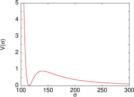
Figure 1: Potential $V\left(\phi\right)$ given by eq. (12), in the units of $10^{-15}M_{Pl}^{4}$. In the minimum $V\sim\left(10^{-4}M_{Pl}\right)^{4}\neq 0$.

However, for a generic initial value of the modulus in the strong coupling, the modulus will fall down the potential and the evolution will be dominated by its very large initial kinetic energy. The potential will remain subleading because it is too steep: its initial role is to just start the phase of kinetic domination. By the time the modulus reaches a minimum, it will have acquired too much kinetic energy from rolling down such a steep potential. As a result the modulus will skip over the barrier and continue rolling towards the weak coupling. This is the origin of the overshoot problem [16]. If such compactifications are to avoid special initial condition, they need a dynamical mechanism which will arrest the modulus before the flyover. Otherwise, it will be extremely hard to see how to ever keep the modulus around the minimum and start early inflation.

The radiation terms $\propto\rho_{rad}$ in (9), (10) can help to slow down the modulus. Their damping effects have been studied in [19] and have been observed earlier in [20, 21]. Because of the conformal symmetry, the stress-energy tensor of radiation vanishes, and so the radiation does not source the modulus. This is manifest in (11) where the radiation terms are absent. Then because radiation scales only as $\rho\sim 1/a^{4}$ it will overtake the scalar kinetic energy, which will damp out as $1/a^{6}$, and the modulus will stop.

We note that the curvature term $k/a^{2}$ will work in a similar vein, but even more efficiently than radiation, if $k=-1$. In that case, the curvature term will begin to dominate the evolution of the universe soon after it came into existence, and lead to the linear expansion $a\sim t$. This will dilute the kinetic term of the scalar even faster than radiation. Thus if either of these terms dominates early on, and the scalar does not overshoot the minimum before it stops to control $H$, it can get caught and inflation could begin. However, in the case of radiation, since the black hole density redshifts only as $1/a^{3}$, it will overtake radiation within few Hubble times after the beginning, and if initial $k$ is small or zero, the black hole gas will play the key role in the evolution of the modulus. In what follows we will therefore ignore the $\rho_{rad}$ and $k/a^{2}$ terms, and instead focus on the black hole contributions $\propto\rho_{BH}$.

To leading order, the effects of the interactions of the modulus with the black hole gas $\rho_{BH}$ can be described as an environment-induced mass term, similar to the interactions discussed in [25], and more recently to the chameleon fields [38] (see also [39]). The presence of this new mass term $\propto\rho_{BH}$ suggests a new method for capturing the scalar in a potential minimum. The interactions with the black hole gas pull it towards $\phi_{*}$ where it awaits for the contributions from the potential $V$ to overtake the black hole terms. When $\phi_{*}$ is divided from the supersymmetric region by a barrier in $V$, the scalar will eventually settle into a minimum of $V$ where inflation can take place. It will not overshoot the barrier since its kinetic energy will be spent against the black hole mass pumping. However this effect in general is not always enough to stabilize the scalar. Indeed, if the gas gets diluted too fast, the interactions will become too weak to dissipate the scalar kinetic energy. This can be seen immediately from the comparison with a simple particle mechanics with a time-dependent mass. For example, if one considers a pendulum with a mass term $m^{2}=\alpha/t^{2}$, one finds that the motion is very unstable, and there are modes which move the pendulum away from the minimum at zero. However, in our case the black holes do not dilute dangerously fast!

To see this, consider a borough of the landscape where the modulus $\phi$ measures the size of the 6D space of a warped compactification of the type IIB theory according to the prescription of [7, 35]. Then the gauge field in (3) can arise from reducing a 10D 3-form such that one index is in the internal space, and so the corresponding choice for ${\tt g}_{2}$ is ${\tt g}_{2}=-\sqrt{2/3}$. Recall that the weak coupling is recovered in the limit $\phi\rightarrow\infty$. Consider (11) with these parameters when the scalar is close to the effective minimum at $\phi_{*}$. The small perturbations $\vartheta=\phi-\phi_{*}$ obey the linearized version of (11). After black holes start to dominate in (9), the solution behaves as $a=t^{2/3}$ and $\rho_{BH}=3M^{2}_{P}H^{2}=4M^{2}_{P}/3t^{2}$. In this limit the linearized equation becomes

$$t^{2}\ddot{\vartheta}+2t\dot{\vartheta}+\frac{2}{9}{\vartheta}=0\,.$$ (13)

The solutions for $\phi$ then are

$$\phi=\phi_{*}+\frac{A}{t^{1/3}}+\frac{B}{t^{2/3}}\,,$$ (14)

and so thanks to Hubble damping the evolution is stable under small perturbations. This is the key ingredient of our mechanism, which guarantees that the scalar entrapment to $\phi_{*}=M_{Pl}\ln(g^{2}_{0}{\langle p\rangle}/{\langle q\rangle})$ is gentle enough to ensure the loss of the scalar kinetic energy.

We have studied the capture of the modulus by the black hole gas numerically in order to verify the stability of the entrapment in the nonlinear regime. In a typical case, the evolution is depicted in Fig. (2). We have taken the initial density of black holes to be $\sim 10^{-3}M_{Pl}^{4}$, a number close to, but safely below the Planck scale, in accordance with our assumptions that $g_{0}\sim{\cal O}(1)$, the validity of the (super)gravity approximation and that the universe emerged near the Planck scale. Since the initial effects of the potential are merely to induce a large kinetic energy of the modulus, early on we can replace it by picking a large initial value of $\dot{\phi}\sim M^{2}_{Pl}$ and set $V=0$. Further because of the Boltzmann suppression in (5) for massive states, it is natural to take the initial value of the black hole energy density to be somewhat lower than $M_{Pl}^{4}$. In this case the modulus kinetic energy will start dominating the universe. However it dilutes fast, and the black hole density starts to contribute quickly. We have assumed here that the initial value of $g$ is of the order of unity, so that the location of the attractor for $\phi$ is near $M_{Pl}$. Clearly, the black holes trap the modulus at a value $\phi_{*}$ and the modulus kinetic energy quickly becomes subdominant.

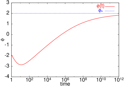
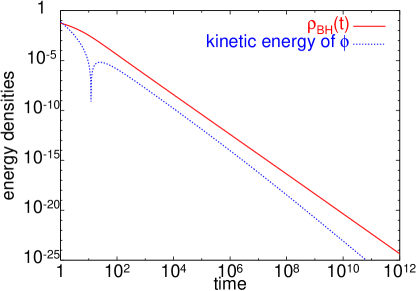
Figure 2: Numerical results for $V=0$. Left: evolution of the field $\phi$, in the units of $M_{Pl}$, as a function of time. We depict time in the units of $M_{Pl}/\sqrt{\rho_{BH~{}0}}$ throughout, and we set $\phi_{*}=2\,M_{Pl}$. The initial conditions are $\phi_{0}=M_{Pl}$, $\dot{\phi}_{0}=-M_{Pl}^{2}$, $\rho_{BH~{}0}=10^{-3}\,M_{Pl}^{4}$ at $t=0$. Right: evolution of $\rho_{BH}$ and the scalar kinetic energy, in the units of $\rho_{BH~{}0}$.

It is possible to verify this behavior analytically. An approximate solution of eqs. (9), (10), (11) initially is given by the FRW cosmology dominated by a massless scalar, where $\phi(t)\sim\sqrt{\frac{2}{3}}\,M_{Pl}\,\ln t$, and $a(t)\sim t^{1/3}$. This ends when the kinetic energy of the scalar redshifts down to the energy density of the black hole gas, roughly at a time $t_{1}\simeq(M_{Pl}/\dot{\phi}_{0})({\dot{\phi}_{0}^{2}}/{\rho_{BH~{}0}})^{3/4}$. Since $\rho_{BH~{}0}$ is below the Planckian density, $\phi$ will have rolled several units of Planck mass until black holes begin to trap it, but not a huge amount. The general dynamics with the black hole terms is not tractable analytically, however we can follow the approach towards the attractor at $\phi_{*}$ as long as $\phi-\phi_{*}\gg M_{Pl}$. In this case we can approximate the $\cosh$ and $\sinh$ functions by exponentials, and find a solution

$$\phi\left(t\right) = \bar{\phi}-\frac{2}{5}\,M_{Pl}\,\log\left(1+\mu\,t\right)\,,$$

$$a\left(t\right) = a_{0}\,\left(1+\mu\,t\right)^{8/15}\,,$$

$${\mathrm{e}}^{\bar{\phi}/\sqrt{6}\,M_{Pl}} = \frac{72}{25}\frac{a_{0}^{3}\,\mu^{2}\,M_{Pl}^{2}}{\rho_{0}}\,.$$ (15)

The dimensionful parameter $\mu$ is determined by the scalar speed $\dot{\phi}$ at the instant when the black holes begin to take over from the scalar kinetic energy. This limiting behavior is consistent with the numerical integration displayed in Fig. (2), describing a slow approach of $\phi$ towards the attractor $\phi_{*}$.

After some time in this regime, the black hole density will have redshifted to near the scale of the potential $V\left(\phi\right)$. If the initial value of $g$ was close to unity, so that ${\langle p\rangle}/{\langle q\rangle}\simeq{\cal O}(1)$, the modulus will remain in the region of $\phi\sim\phi_{*}\sim{\cal O}(M_{Pl})$ where the minima of $V(\phi)$ are located. The modulus will slide down the slope of $V\left(\phi\right)$ gently, eventually settling down in the minimum and starting an inflationary era (if the value of $V$ at the minimum is nonzero, or if the approach to the minimum is along a very flat slope, where $m_{\phi}<H$). We plot a typical evolution of the modulus towards the minimum in Fig. (3). This kind of behavior is generic whenever the initial black hole density is not too small, and when $\phi_{*}\sim{\cal O}(M_{Pl})$, so that the black hole $\phi_{*}$ point lies in the basin of attraction of a minimum of $V$.

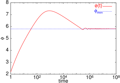
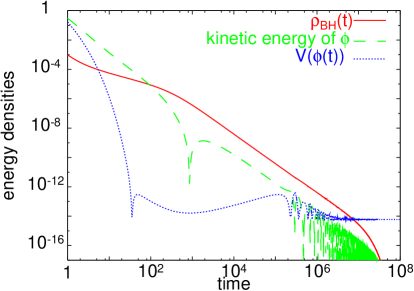
Figure 3: As in Fig. (2), but with nonvanishing potential $V\left(\phi\right)$ given by eq. (12). Again $\rho_{BH~{}0}=10^{-3}\,M_{Pl}^{4}$. At the time $\sim 10^{6}$ the modulus gets trapped in the local minimum of $V$ located at $\phi_{\mathrm{min}}\simeq 5.8\,M_{Pl}$.

In the case when the initial value of $\rho_{BH}$ is too small, or if the attractor $\phi_{*}$ is far too far in the weak coupling regime, the modulus will not be trapped in the minimum of the potential $V\left(\phi\right)$. Either the potential will become important too early, before the black hole gas manages to slow down the modulus, or $\phi_{*}$ will lie outside of the basin of attraction of the minima of $V$. In each of these cases the modulus will overshoot the minimum at $\phi_{\mathrm{min}}$ and will forever continue rolling down the slope $V\left(\phi\right)$ towards the weak coupling. In such situations the Brustein-Steinhardt problem cannot be avoided and inflation will not start. The system will eventually converge to a tracking regime (analogous to the one observed for exponential potentials in quintessence models). A typical representative of this behavior is displayed in Fig. (4).

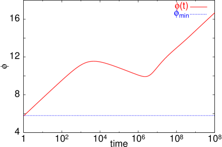
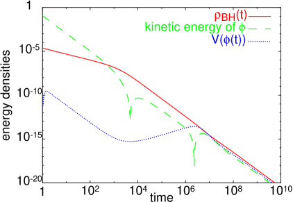
Figure 4: Here we take $\rho_{BH~{}0}=10^{-6}\,M_{Pl}^{4}$. Now the number of black holes is not sufficient to stabilize the modulus and $\phi$ overshoots the minimum at $\phi_{\mathrm{min}}$.

However in those cases when the universe is created very close to the Planck scale, as would typically occur in for example the approach advocated in [17], the initial black hole density will be significant. This is simply because of equipartition and equivalence principle. Hence the moduli would be captured quickly in the black hole attractor $\phi_{*}$. It still remains that in the regions of the landscape where the initial value of the coupling was too small, $\phi_{*}$ would end up outside of the basin of attraction and the modulus would still run off to the weak coupling eventually. However, this behavior is endemic for the small initial coupling regardless of the subsequent dynamics. If the coupling had started off too small, the modulus would never have had a chance of ending in the minimum of $V(\phi)$ anyway. It would always fall out of the basin of attraction of the minima of $V$. Thus this initial regime is of very little interest to start with. One has to make some choices of the initial conditions, and the whole purpose of the resolutions of the overshoot problem here and in [19, 20, 21, 26, 27] is to demonstrate that the favorable initial region may be likely: in this case, it is a finite interval of the vevs of $\phi$. In the landscape, at very high scales where the influence of the potential is negligible, the initial value of $\phi$ may be anything, and so there will be many regions where $\phi\sim{\cal O}(M_{Pl})$. In these regions our mechanism will work in a natural way, and they will inflate. The a posteriori probability to be in such regions will then be large because they will become exponentially big after inflation.

Once inflation starts, the gas of black holes will dilute exponentially quickly. By the time inflation is over, assuming it produces about 65 e-folds or so, the number density of the black holes will drop by a factor of about $10^{90}$. If inflation happens near the GUT scale, say $V^{1/4}\sim 10^{15}{\rm GeV}$, the final number density of black holes at the end of inflation will be

$$n_{BH~{}final}\leq 10^{-90}\frac{V}{M_{Pl}}\sim 10^{-22}{\rm eV}^{3}\,.$$ (16)

After inflation, the universe will expand roughly for another factor of $10^{90}$ until it reaches the present epoch. The number density of these primordial black holes today will therefore be no more than about $n_{BH~{}final}({\rm today})~{}\mbox{\raisebox{-2.58334pt}{$\stackrel{{\scriptstyle<}}{{\sim}}$}}~{}10^{-112}{\rm eV}^{3}$, leaving us with at most one such black hole per more than $10^{13}$ present horizon volumes. In other words, these primordial black holes will become just as efficiently diluted as the primordial monopoles in the original formulation of inflation [1]. They will quietly go away after completing their task.

To summarize, in this paper we have proposed a new method for resolving the Brustein-Steinhardt moduli overshoot problem [16] in string cosmology. We find that a gas of primordial black holes in the early universe, where the mass of black holes depends on the modulus, can provide a transient attractor for the modulus. When such black holes are produced they will trap the modulus temporarily, and keep it within the basin of attraction of the minima of the nonperturbative modulus potential $V$. As time goes on, the black hole density will redshift away, placing the modulus gently on the potential slope. Following this the modulus will slowly settle into the minimum, where it can drive inflation. A key ingredient of our mechanism is that the universe should be created near the Planck scale, so that the heavy states are produced initially with non-negligible number density. Such an approach has been proposed recently in [17], and our mechanism may be a natural ingredient for helping the modulus stop in the inflationary valleys in the landscape. After inflation has begun, the density of black holes redshifts away to exponentially small numbers, just like the density of heavy monopoles in the early models of inflation. These black holes are pushed outside of the current horizon. We stress that our mechanism relies mainly on the presence of heavy states in the theory whose mass depends on the modulus. It may be possible to realize a similar mechanism in other regimes, using different massive states. It would be interesting to consider such mechanisms in other cosmological models, where for example the initial density of massive states could be small, but the minima of the potential lie at very large vevs, such as in the theories with low scale unification.

Acknowledgements

We thank R. Brustein, S. Dimopoulos, R. Kallosh, L. Kofman, A. Linde and S. Thomas for useful discussions. NK and LS thank the Aspen Center for Physics for a kind hospitality during the course of this work. The work of NK and LS was supported in part by the DOE Grant DE-FG03-91ER40674, in part by the NSF Grant PHY-0332258 and in part by a Research Innovation Award from the Research Corporation.

References

- [1] A. Guth, Phys. Rev. D 23 (1981) 347; A. Linde, Phys. Lett. B 108 (1982) 389; A. Albrecht and P. Steinhardt, Phys. Rev. Lett. 48 (1982) 1220.
- [2] A. D. Linde, Phys. Lett. B 162 (1985) 281; A. Albrecht, R. H. Brandenberger and R. Matzner, Phys. Rev. D 35 (1987) 429; S. W. Hawking and D. N. Page, Nucl. Phys. B 298 (1988) 789; A. Vilenkin, Phys. Rev. D 37 (1988) 888; D. S. Goldwirth and T. Piran, Phys. Rept. 214 (1992) 223; L. Dyson, M. Kleban and L. Susskind, JHEP 0210 (2002) 011; T. Banks, W. Fischler and S. Paban, JHEP 0212 (2002) 062.
- [3] P. J. Steinhardt, in The Very Early Universe, eds: G. W. Gibbons, S. W. Hawking, and S. T. C. Siklos (Cambridge University Press, 1983), pp. 251–266.
- [4] A. Vilenkin, Phys. Rev. D 27 (1983) 2848.
- [5] A. Linde, Phys. Lett. B 129 (1983) 177; Mod. Phys. Lett. A 1 (1986) 81.
- [6] A. H. Guth, Phys. Rept. 333 (2000) 555.
- [7] S. Kachru, R. Kallosh, A. Linde and S. P. Trivedi, Phys. Rev. D 68 (2003) 046005.
- [8] S. Kachru, R. Kallosh, A. Linde, J. Maldacena, L. McAllister and S. P. Trivedi, JCAP 0310 (2003) 013.
- [9] J. J. Blanco-Pillado, C. P. Burgess, J.M. Cline, C. Escoda, M. Gomez-Reino, R. Kallosh, A. Linde and F. Quevedo, hep-th/0406230.
- [10] R. Bousso and J. Polchinski, JHEP 0006 (2000) 006.
- [11] L. Susskind, hep-th/0302219; hep-ph/0406197; B. Freivogel and L. Susskind, hep-th/0408133.
- [12] M. R. Douglas, JHEP 0305 (2003) 046. S. Ashok and M. R. Douglas, JHEP 0401 (2004) 060; A. Giryavets, S. Kachru and P. K. Tripathy, JHEP 0408, 002 (2004).
- [13] N. Arkani-Hamed and S. Dimopoulos, hep-th/0405159; M. R. Douglas, hep-th/0405279; G. F. Giudice and A. Romanino, hep-ph/0406088; M. Dine, E. Gorbatov and S. Thomas, hep-th/0407043.
- [14] K. Behrndt and S. Forste, Nucl. Phys. B 430 (1994) 441; A. Lukas, B. A. Ovrut and D. Waldram, Phys. Lett. B 393 (1997) 65; Nucl. Phys. B 495 (1997) 365; N. Kaloper, Phys. Rev. D 55 (1997) 3394; H. Lu, S. Mukherji, C. N. Pope and K. W. Xu, Phys. Rev. D 55 (1997) 7926; J. E. Lidsey, D. Wands and E. J. Copeland, Phys. Rept. 337 (2000) 343.
- [15] P. Binetruy and M. K. Gaillard, Phys. Rev. D 34 (1986) 3069.
- [16] R. Brustein and P. J. Steinhardt, Phys. Lett. B 302 (1993) 196.
- [17] A. Linde, hep-th/0408164.
- [18] D. H. Coule and J. Martin, Phys. Rev. D 61 (2000) 063501.
- [19] R. Brustein, S. P. de Alwis and P. Martens, hep-th/0408160.
- [20] N. Kaloper and K. A. Olive, Astropart. Phys. 1 (1993) 185.
- [21] A. A. Tseytlin and C. Vafa, Nucl. Phys. B 372 (1992) 443; A. A. Tseytlin, hep-th/9206067.
- [22] C. Wetterich, Nucl. Phys. B 302 (1988) 645; Nucl. Phys. B 324 (1989) 141.
- [23] S. Kalara, N. Kaloper and K. A. Olive, Nucl. Phys. B 341 (1990) 252; J. A. Casas, J. Garcia-Bellido and M. Quiros, Nucl. Phys. B 361 (1991) 713.
- [24] T. Banks, M. Berkooz, S. H. Shenker, G. W. Moore and P. J. Steinhardt, Phys. Rev. D 52 (1995) 3548.
- [25] T. Damour and K. Nordtvedt, Phys. Rev. Lett. 70 (1993) 2217; Phys. Rev. D 48 (1993) 3436; T. Damour and A. M. Polyakov, Nucl. Phys. B 423 (1994) 532; Gen. Rel. Grav. 26 (1994) 1171.
- [26] T. Barreiro, B. de Carlos and E. J. Copeland, Phys. Rev. D 58 (1998) 083513.
- [27] G. Huey, P. J. Steinhardt, B. A. Ovrut and D. Waldram, Phys. Lett. B 476 (2000) 379.
- [28] L. Parker, Phys. Rev. Lett. 21 (1968) 562; Phys. Rev. 183 (1969) 1057; Phys. Rev. D 3 (1971) 346.
- [29] Y. B. Zeldovich and A. A. Starobinsky, Sov. Phys. JETP 34 (1972) 1159.
- [30] S. Ferrara, R. Kallosh and A. Strominger, Phys. Rev. D 52 (1995) 5412; S. Ferrara and R. Kallosh, Phys. Rev. D 54 (1996) 1514; Phys. Rev. D 54 (1996) 1514.
- [31] G. W. Gibbons, Nucl. Phys. B 207 (1982) 337; G. W. Gibbons and K. i. Maeda, Nucl. Phys. B 298 (1988) 741; D. Garfinkle, G. T. Horowitz and A. Strominger, Phys. Rev. D 43 (1991) 3140 [Erratum-ibid. D 45 (1992) 3888].
- [32] R. Kallosh, A. D. Linde, T. Ortin, A. W. Peet and A. Van Proeyen, Phys. Rev. D 46 (1992) 5278.
- [33] M. J. Duff and J. Rahmfeld, Phys. Lett. B 345 (1995) 441; J. Rahmfeld, Phys. Lett. B 372 (1996) 198.
- [34] A. V. Frolov and L. Kofman, JCAP 0305 (2003) 009.
- [35] S. B. Giddings, S. Kachru and J. Polchinski, Phys. Rev. D 66 (2002) 106006.
- [36] R. Kallosh and A. D. Linde, Phys. Rev. D 56 (1997) 3509.
- [37] R. C. Ferrell and D. M. Eardley, Phys. Rev. Lett. 59 (1987) 1617; K. Shiraishi, Nucl. Phys. B 402 (1993) 399.
- [38] J. Khoury and A. Weltman, astro-ph/0309300; Phys. Rev. D 69 (2004) 044026; P. Brax, C. van de Bruck, A. C. Davis, J. Khoury and A. Weltman, astro-ph/0408415.
- [39] S. Alexander, R. H. Brandenberger and D. Easson, Phys. Rev. D 62 (2000) 103509; R. Easther, B. R. Greene, M. G. Jackson and D. Kabat, JCAP 0401 (2004) 006; S. Watson and R. Brandenberger, JCAP 0311 (2003) 008; J. Y. Kim, hep-th/0403096; D. Stojkovic and K. Freese, hep-ph/0403248; S. Watson, hep-th/0404177.